5 ELECTRICITY AND MAGNETISM - Weebly

169

5 E L E C T R I C I T Y A N D M A G N E T I S MIntroductionModern society uses a whole range of electrical devices from the simplest heated metal filaments that provide light, through to the most sophisticated medical instruments and computers. Devices of increasing technical complexity are developed every day.

In this topic we look at the phenomenon of electricity, and what is meant by charge and electric current. We consider the three effects that can be observed when charge flows in an electric circuit.

5.1 Electric fields

Nature of scienceElectrical theory resembles the kinetic theory of gases in that a theory of the microscopic was developed to explain the macroscopic observations that had been made over centuries. The development of this subject and some of the byways that were taken make this a fascinating study. We should remember the many scientists who were involved. It is a tribute to them that they could make so much progress when the details of the microscopic nature of electronic charge were unknown to them.

Understanding Charge Electric field Coulomb’s law Electric current Direct current (dc) Potential difference (pd)

Applications and skills Identifying two species of charge and the

direction of the forces between them Solving problems involving electric fields and

Coulomb’s law Calculating work done when charge moves in

an electric field in both joules and electronvolts Identifying sign and nature of charge carriers in

a metal Identifying drift speed of charge carriers Solving problems using the drift-speed equation Solving problems involving current, potential

difference, and charge

Equations current-charge relationship: I = ∆q

______ ∆t

Coulomb's law: F = k q1 q2 ________

r2

the coulomb constant: k = 1 ________ 4πε0

potential difference definition: V = W ____ q

conversion of energy in joule to electron-volt: W(J) ≡ W(eV)

__________ e electric field strength: E = F ___ q drift speed: I = nAvq

Charge and fieldSimple beginningsTake a plastic comb and pull it through your hair. Afterwards, the comb may be able to pick up small pieces of paper. Look closely and you may see the paper being thrown off shortly after touching the comb.

Similar observations were made early in the history of science. The discovery that objects can be charged by friction (you were doing this when you drew the comb through your hair) is attributed to the Greek scientist Thales who lived about 2600 years ago. In those days, silk was spun on amber spindles and as the amber rotated and rubbed against its bearings, the silk was attracted to the amber. The ancient Greek word for amber is ηλεκτρον (electron).

In the 1700s, du Fay found that both conductors and insulators could be “electrified” (the term used then) and that there were two opposite kinds of “electrification”. However, he was unable to provide any explanation for these effects. Gradually, scientists developed the idea that there were two separate types of charge: positive and negative. The American physicist, Benjamin Franklin, carrying out a famous series of experiments flying kites during thunderstorms, named the charge on a glass rod rubbed with silk as “positive electricity”. The charge on materials similar to ebonite (a very hard form of rubber) rubbed with animal fur was called “negative”. One of Franklin’s other discoveries was that a charged conducting sphere has no electric field inside it (the field and the charges always being outside the sphere). Joseph Priestley was able to deduce from this that the force between two charges is inversely proportional to the square of the distance between the charges.

At the end of the nineteenth century J. J. Thomson detected the presence of a small particle that he called the electron. Experiments showed that all electrons have the same small quantity of charge and that electrons are present in all atoms. Atoms were found to have protons that have the same magnitude of electronic charge as, but have opposite charge to, the electron. In a neutral atom or material the number of electrons and the number of protons are equal. We now assign a negative charge to the electron and positive to the proton. There are only these two species of charge.

Explaining electrostaticsExperiments also show that positively charged objects are attracted to negatively charged objects but repelled by any other positively charged object. The possible cases are summed up in figure 1. There can also be an attraction between charged and uncharged objects due to the separation of charge in the uncharged object. In figure 1(c) the electrons in the uncharged sphere are attracted to the positively charged sphere (sphere A) and move towards it. The electrons in sphere B are now closer to the positives in sphere A than the fixed positive charges on B. So the overall force is towards sphere A as the force between two charges increases as the distance between them decreases.

170

5 E L E C T R I C I T Y A N D M A GN E T I S M

+

+

+ ++

++

+

−

− −−

−−

−−

opposite charges attract(a)

neutral

+

+ ++

++

++ +

+

+ ++

++

+

like charges repel(b)

charge separation means that attraction occurs(c)

−−

−−−−−−

−−

−−−

−−

− −−

++ +

+

++

+-

+

Figure 1 Attractions between charges.

We now know that the simple electrostatic effects early scientists observed are due only to the movement of the negatively charged electrons. An object with no observed charge has an exact balance between the electrons and the positively charged protons; it is said to be neutral. Some electrons in conducting materials are loosely attached to their respective atoms and can leave the atoms to move from one object to another. This leaves the object that lost electrons with an overall positive charge. The electrons transferred give the second object an overall negative charge. Notice that electrons are not lost in these transfers. If 1000 electrons are removed from a rod when the rod is charged by a cloth, the cloth will be left with 1000 extra electrons at the end of the process. Charge is conserved; the law of conservation of charge states that in a closed system the amount of charge is constant.

When explaining the effects described here, always use the idea of surplus of electrons for a negative charge, and describe positive charge in terms of a lack (or deficit) of electrons. Figure 2 shows how an experiment to charge a metal sphere by induction is explained.

++

+++

+−−−

−

−−−−−−−

− −

charged rodseparates charge

sphere is earthedand electrons arerepelled to Earth

Earth connection broken,rod removed, and electrons

re-distributed to leave spherepositive after rearrangement

conducting sphere

insulating stand6 electrons travel to Earth

removecharged rod

++

+++ ++

++

+

+

+

−−−−−−−

connected to Earth

Figure 2 Charging by induction.

TOK

Inverse-square laws

Forces between charged objects is one of several examples of inverse-square laws that you meet in this course. They are of great importance in physics. Inverse-square laws model a characteristic property of some fields, which is that as distance doubles, observed effects go down by one quarter.

Mathematics helps you to learn and conceptualize your ideas about the subject. When you have learnt the physics of one situation (here, electrostatics) then you will be able to apply the same rules to new situations (for example, gravitation, in the next topic).

Is the idea of field a human construct or does it reflect the reality of the universe?

171

5 . 1 E L E C T R I C F I E L D S

Measuring and defining chargeThe unit of charge is the coulomb (abbreviated to C). Charge is a scalar quantity.

The coulomb is defined as the charge transported by a current of one ampere in one second.

Measurements show that all electrons are identical, with each one having a charge equal to –1.6 × 10–19 C; this fundamental amount of charge is known as the electronic (or elementary) charge and given the symbol e.

Charges smaller than the electronic charge are not observed in nature. (Quarks have fractional charges that appear as ± 1 __ 3 e or ± 2 __ 3 e; however, they are never observed outside their nucleons.)

In terms of the experiments described here, the coulomb is a very large unit. When a comb runs through your hair, there might be a charge of somewhere between 1 pC and 1 nC transferred to it.

Forces between charged objectsIn 1785, Coulomb published the first of several Mémoires in which he reported a series of experiments that he had carried out to investigate the effects of forces arising from charges.

He found, experimentally, that the force between two point charges separated by distance r is proportional to 1 __

r2 thus confirming the earlier theory of Priestley. Such a relationship is known as an inverse-square law.

Investigate!Forces between charges

These are sensitive experiments that need care and a dry atmosphere to achieve a result.

Take two small polystyrene spheres and paint them with a metal paint or colloidal graphite, or cover with aluminum foil. Suspend one from an insulating rod using an insulating (perhaps nylon) thread. Mount the other on top of a sensitive top-pan balance, again using an insulating rod.

Charge both spheres by induction when they are apart from each other. An alternative charging method is to use a laboratory high voltage power supply. Take care, your teacher will want to give you instructions about this.

Bring the spheres together as shown in figure 3 and observe changes in the reading on the balance.

insulating support

insulating rod

sensitive top-panbalance

−

+

Figure 3

172


d ∝ sideways force on ballr = distance between balls

d

r

Figure 4

Another method is to bring both charged spheres together as shown in figure 4.

The distance d moved by the sphere depends on the force between the charged spheres. The distance r is the distance between the centres of the spheres.

Vary d and r making careful measurements of them both.

Plot a graph of d against 1 __ r2 . An experiment

performed with care can give a straight-line graph.

For small deflections, d is a measure of the force between the spheres (the larger the force the greater the distance that the sphere is moved) whereas r is the distance between sphere centres.

Nature of scienceScientists in Coulomb’s day published their work in a very different way from scientists today. Coulomb wrote his results in a series of books called Mémoires. Part of Coulomb’s original Mémoire in which he states the result is shown in figure 5.

Figure 5

Later experiments confirmed that the force is proportional to the product of the size of the point charges q1 and q2.

Combining Coulomb’s results together with these gives

F ∝ q1 q2 _ r2

where the symbol ∝ means “is proportional to”.

The magnitude of the force F between two point charges of charge q1 and q2 separated by distance r in a vacuum is given by

F = kq1 q2 _ r2

where k is the constant of proportionality and is known as Coulomb’s constant.

In fact we do not always quote the law in quite this mathematical form. The constant is frequently quoted differently as

k = 1 _ 4πε0

The new constant ε0 is called the permittivity of free space (free space is an older term for “vacuum”. The 4π is added to rationalize electric and

173


magnetic equations – in other words, to give them a similar shape and to retain an important relationship between them (see the TOK section on page 177).

So the equation becomes

F = 1 _ 4πε0

q1 q2 _ r2

When using charge measured in coulombs and distance measured in metres, the value of k is 9 × 109 N m2 C–2.

This means that ε0 takes a value of 8.854 × 10–12 C2 N–1 m–2 or, in fundamental units, m–3 kg–1 s4 A2.

The equation as it stands applies only for charges that are in a vacuum. If the charges are immersed in a different medium (say, air or water) then the value of the permittivity is different. It is usual to amend the equation slightly too, k becomes 1

___ 4πε as the “0” subscript in ε0 should only be used for the vacuum case. For example, the permittivity of water is 7.8 × 10–10 C2 N–1 m–2 and the permittivity of air is 8.8549 × 10–12 C2 N–1 m–2. The value for air is so close to the free-space value that we normally use 8.85 × 10–12 C2 N–1 m–2 for both. The table gives a number of permittivity values for different materials.

Material Permittivity / 10–12 C2 N–1 m–2

paper 34rubber 62water 779graphite 106diamond 71

This equation appears to say nothing about the direction of the force between the charged objects. Forces are vectors, but charge and (distance)2 are scalars. There are mathematical ways to cope with this, but for point charges the equation gives an excellent clue when the signs of the charges are included.

force on Bdue to A

positive direction

force on Adue to B charge

Acharge

B

r

Figure 6 Force directions.

We take the positive direction to be from charge A to charge B; in figure 6 that is from left to right. Let’s begin with both charge A and charge B being positive. When two positive charges are multiplied together in

q1 q2 ____ r2 , the resulting sign of the force acting on charge B due to

charge A is also positive. This means that the direction of the force will be assigned the positive direction (from charge A to charge B): in other words, left to right. This agrees with the physics because the charges are repelled. If both charges are negative then the answer is the same, the charges are repelled and the force is to the right.

174


Electric fieldsSometimes the origin of a force between two objects is obvious, an example is the friction pad in a brake rubbing on the rim of a bicycle wheel to slow the cycle down. In other cases there is no physical contact between two objects yet a force exists between them. Examples of this include the magnetic force between two magnets and the electrostatic force between two charged objects. Such forces are said to “act at a distance”.

The term field is used in physics for cases where two separated objects exert forces on each other. We say that in the case of the comb picking up the paper, the paper is sitting in the electric field due to the comb. The concept of the field is an extremely powerful one in physics not least because there are many ideas common to all fields. As well as the magnetic and electrostatic fields already mentioned, gravity fields also obey the same rules. Learn the underlying ideas for one type of field and you have learnt them all.

Worked examples1 Two point charges of +10 nC and –10 nC in

air are separated by a distance of 15 mm.

a) Calculate the force acting between the two charges.

b) Comment on whether this force can lift a small piece of paper about 2 mm × 2 mm in area.

Solutiona) It is important to take great care with the

prefixes and the powers of ten in electrostatic calculations.

The charges are: +10 × 10–9 C and –10 × 10–9 C. The separation distance is 1.5 × 10–2 m (notice how the distance is converted right at the outset into consistent units).

So F = (+1 × 10–8) × (–1 × 10–8) ___

4πε0 (1.5 ×10–2)2

= 4.0 × 10–3 N

The charges are attracted along the line joining them. (Do not forget that force is a vector and needs both magnitude and direction for a complete answer.)

b) A sheet of thin A4 paper of dimensions 210 mm by 297 mm has a mass of about 2 g. So the small area of paper has a mass of about 1.3 × 10–7 kg and therefore a weight of 1.3 × 10–6 N. The electrostatic force could lift this paper easily.

2 Two point charges of magnitude +5 µC and +3 µC are 1.5 m apart in a liquid that has a permittivity of 2.3 × 10–11 C2 N–1 m–2.

Calculate the force between the point charges.

Solution

F = (+5 ×10–6) × (+3 × 10–6)

__________________ 4π × 2.3 × 10–11 × (1.5)2 = 23 mN;

a repulsive force acting along the line joining the charges.

If, however, one of the charges is positive and the other negative, then the product of the charges is negative and the force direction will be opposite to the left-to-right positive direction. So the force on charge 2 is now to the left. Again, this agrees with what we expect, that the charges attract because they have opposite signs.

175


Mapping fields

Investigate!Plotting electric fields

+ −

castor oilsemolina

(a)

(b)

(c)

Figure 7

At an earlier stage in your school career you may have plotted magnetic field patterns using iron filings (if you have not done this there is an Investigate! in Sub-topic 5.4 to illustrate

the method). This experiment allows patterns to be observed for electric fields.

Put some castor oil in a Petri dish and sprinkle some grains of semolina (or grits) onto the oil. Alternatives for the semolina include grass seed and hairs cut about 1 mm long from an artist paint brush.

Take two copper wires and bend one of them to form a circle just a little smaller than the internal diameter of the Petri dish. Place the end of the other wire in the centre of the Petri dish.

Connect a 5 kV power supply to the wires – take care with the power supply!

Observe the grains slowly lining up in the electric field.

Sketch the pattern of the grains that is produced.

Repeat with other wire shapes such as the four shown in figure 7(c).

−−−

−−−−−−−−

+++

++++++++

− +

−−−−−−

+

−

−−−

−−

−−

+

Figure 8 Electric field patterns.

In the plotting experiment, the grains line up in the field that is produced between the wires. The patterns observed resemble those in figure 8. The experiment cannot easily show the patterns for charges with the same sign.

The idea of field lines was first introduced by Michael Faraday (his original idea was of an elastic tube that repelled other tubes). Although field lines are imaginary, they are useful for illustrating and understanding the nature of a particular field. There are some conventions for drawing these electric field patterns.

The lines start and end on charges of opposite sign.

An arrow is essential to show the direction in which a positive charge would move (i.e. away from the positive charge and towards the negative charge).

Where the field is strong the lines are close together. The lines act to repel each other.

The lines never cross.

The lines meet a conducting surface at 90°.

176


TOK

So why not use k?

James Maxwell, working in the middle of the nineteenth century, realized that there was an important connection between electricity, magnetism and the speed of light. In particular he was able to show that the permittivity of free space ε0 (which relates to electrostatics) and the permeability of free space -0 (which relates to electromagnetism) are themselves connected to the speed of light c:

1 ________ ε0µ0 = c2

This proves to be an important equation. So much so that, in the set of equations that arise from the SI units we use, we choose to use ε0 in all the electrostatics equations and µ0 in all the magnetic equations.

However, not all unit systems choose to do this. There is another common system, the cgs system (based on the centimetre, the gram and the second, rather than the metre, kilogram and second). In cgs, the value of the constant k in Coulomb’s law is chosen to be 1 and the equation appears as F =

q1 q2 ________ r2 . If the

numbers are different, is the physics the same?

Electric field strengthAs well as understanding the field pattern, we need to be able to measure the strength of the electric field. The electric field strength is defined using the concept of a positive test charge. Imagine an isolated charge Q sitting in space. We wish to know what the strength of the field is at a point P, a distance r away from the isolated charge. We put another charge, a positive test charge of size q, at P and measure the force F that acts on the test charge due to Q. Then the magnitude of the electric field strength is defined to be

E = F _ q

+Q

+q

test charge, P

electric force

r

Figure 9 Definition of electric field strength.

The units of electric field strength are N C–1. (Alternative units, that have the same meaning, are V m–1 and will be discussed in Topic 11.) Electric field strength is a vector, it has the same direction as the force F (this is because the charge is a scalar which only “scales” the value of F up or down). A formal definition for electric field strength at a point is the force per unit charge experienced by a small positive point charge placed at that point.

Coulomb’s law can be used to find how the electric field strength varies with distance for a point charge.

Q is the isolated point charge and q is the test charge, so

F = 1 _ 4πε0

Qq

_ r2

E = F _ q

Therefore

E = 1 _ 4πε0

Qq

_ r2

× 1 _ q

so

E = 1 _ 4πε0

Q

_ r2

The electric field strength of the charge at a point is proportional to the charge and inversely proportional to the square of the distance from the charge.

If Q is a positive charge then E is also positive. Applying the rule that r is measured from the charge to the test charge, then if E is positive it acts outwards away from the charge. This is what we expect as both charge and test charge are positive. When Q is negative, E acts towards the charge Q.

The field shape for a point charge is known as a radial field. The field lines radiate away (positive) or towards (negative) the point charge as shown in figure 10.

−+ Q −Q

Figure 10 Radial fields for positive and negative point charges.

177


The electric field strengths can be added using either a calculation or a scale diagram as outlined in Topic 1.

test charge

field due to -q -q field

field due to +Qnet

electric field

+Q -qgives

+q field

netelectric fieldgives gives

field due to 1 field due to 2

field due to 1 and 2

field due to 3 field due to 3

charge 3

charge 2 charge 1

test charge

+Q

=

+2Q

+Q

Figure 11 Vector addition of electric fields.

This vector addition of field strengths (figure 11) can give us an insight into electric fields that arise from charge configurations that are more complex than a single point charge.

Close to a conductorImagine going very close to the surface of a conductor. Figure 12 shows what you might see. First of all, if we are close enough then the surface will appear flat (in just the same way that we are not aware of the curvature of the Earth until we go up in an aircraft). Secondly we would see that all the free electrons are equally spaced. There is a good reason for this: any one electron has forces acting on it from the other electrons. The electron will accelerate until all these forces balance out and it is in equilibrium, for this to happen they must be equally spaced.

Now look at the field strength vectors radiating out from these individual electrons. Parallel to the surface, these all cancel out with each other so there is no electric field in this direction. (This is the same as saying that any one electron will not accelerate as the horizontal field strength is

Worked examples1 Calculate the electric field strengths in a

vacuum

a) 1.5 cm from a +10 µC charge

b) 2.5 m from a –0.85 mC charge

Solutiona) Begin by putting the quantities into consistent

units: r = 1.5 × 10–2 m and Q = 1.0 × 10–5 C.

Then E = 1.0 × 10–5

____________ 4πε0 (1.5 × 10–2)2 = + 4.0 ×108 N C–1.

The field direction is away from the positive charge.

b) E = –8.5 × 10–4 __

4πε0 (2.5)2 = –1.2 × 106 N C–1

The field direction is towards the negative charge.

2 An oxygen nucleus has a charge of +8e. Calculate the electric field strength at a distance of 0.68 nm from the nucleus.

SolutionThe charge on the oxygen nucleus is 8 × 1.6 × 10–19 C; the distance is 6.8 × 10–10 m.

E = 1.3 × 10–18

_______________ 4πε0 × (6.8 × 10–10)2 = –2.5 ×1010 N C–1 away from

the nucleus.

178


zero). Perpendicular to the surface, however, things are different. Now the field vectors all add up, and because there is no field component parallel to the surface, the local field must act at 90° to it.

So, close to a conducting surface, the electric field is at 90° to the surface.

Conducting sphereThis can be taken a step further for a conducting sphere, whether it is hollow or solid. Again, the free electrons at the surface are equally spaced and all the field lines at the surface of the sphere are at 90° to it. The consequence is that the field must be radial, just like the field of an isolated point charge. So, to a test charge outside the sphere, the field of the sphere appears exactly the same as that of the point charge. Mathematical analysis shows that outside a sphere the field indeed behaves as though it came from a point charge placed at the centre of the sphere with a charge equal to the total charge spread over the sphere.

(Inside the sphere is a different matter, it turns out that there is no electric field inside a sphere, hollow or solid, a result that was experimentally determined by Franklin.)

TOK

But does the test charge affect the original field?

If we wanted to use the definition of the strength of an electric field practically by using a test charge, we would have to take care. Just as a thermometer alters the temperature of the object it measures, so the test charge will exert a force on the original charge (the one with the field we are trying to measure) and may accelerate it, or disturb the field lines. This means in practice that a test charge is really an imaginary construct that we use to help our understanding. In practice we prefer to measure electric field strengths using the idea that it is the potential gradient, in other words the change in the voltage divided by the change in distance: the larger this value, the greater the field strength. We will leave further discussion of this point to Topic 11 but it is food for thought from a theory of knowledge perspective: a measurement that we can think about but not, in practice, carry out. The German language has a name for it: gedankenexperiment “thought experiment”. How can a practical subject such as a science have such a thing?

surface

− − surface

leaving electric field onlyperpendicular to surface

perpendicularto surface add

parallel tosurface cancel

− −

Figure 12 Close to conducting surfaces.

Worked exampleTwo point charges, a +25 nC charge X and a +15 nC charge Y are separated by a distance of 0.5 m.

a) Calculate the resultant electric field strength at the midpoint between the charges.

b) Calculate the distance from X at which the electric field strength is zero.

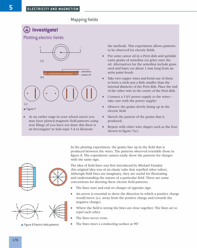
c) Calculate the magnitude of the electric field strength at the point P on the diagram. X and Y are 0.4 m and 0.3 m from P respectively.

P

X Y

0.3 m0.4 m

179


Solution a) EA = 2.5 × 10–8

__ 4πε0 × 0.252

= 3600 N C–1

EB = 1.5 × 10–8 __

4πε0 × 0.252 = 2200 N C–1

The field strengths act in opposite directions, so the net electric field strength is (3600 – 2200) = 1400 N C–1; this is directed away from X towards Y.

b) For E to be zero, EA = –EB and so

2.5 × 10–8 _

4πε0 × d2 = 1.5 × 10–8

__ 4πε0 × (0.5 – d)2

thus

d2 _

(0.5 – d)2 = 2.5 _

1.5

or

d _ (0.5 – d)

= √____ 2.5 _

1.5 = 1.3

d = 0.65 – 1.3d

2.3d = 0.65

d = 0.28 m

c) PX = 0.4 m so EX at P is 2.5 × 10–8

________ 4πε0 × 0.42

= 1400 N C–1 along XP in the direction

away from X.

PY = 0.3 m so EY at P is 1.5 × 10–8

________ 4πε0 × 0.32

= 1500 N C–1 along PY in the direction

towards Y.

P

X

Y

net electric field

The magnitude of the resultant electric field strength is √

___________ 14002 + 15002 = 2100 N C–1

(The calculation of the angles was not required in the question and is left for the reader.)

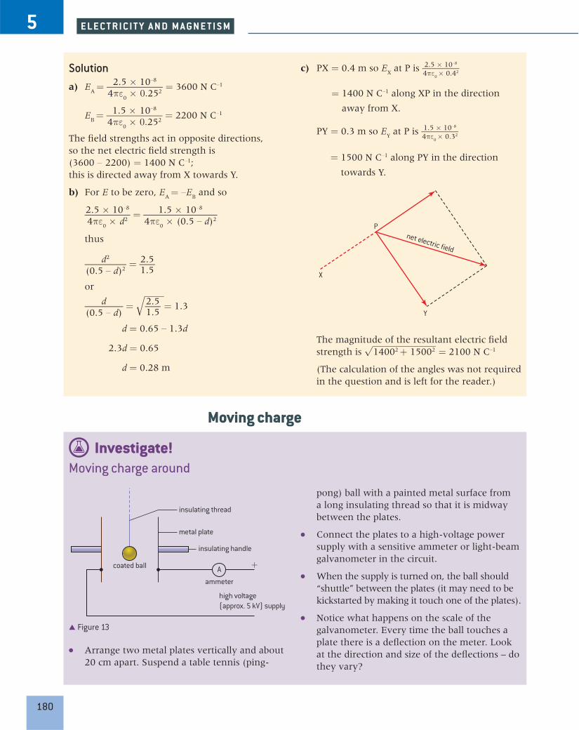
Investigate!Moving charge around

Aammeter

high voltage(approx. 5 kV) supply

metal plate

+coated ball

insulating thread

insulating handle

Figure 13

Arrange two metal plates vertically and about 20 cm apart. Suspend a table tennis (ping-

pong) ball with a painted metal surface from a long insulating thread so that it is midway between the plates.

Connect the plates to a high-voltage power supply with a sensitive ammeter or light-beam galvanometer in the circuit.

When the supply is turned on, the ball should “shuttle” between the plates (it may need to be kickstarted by making it touch one of the plates).

Notice what happens on the scale of the galvanometer. Every time the ball touches a plate there is a deflection on the meter. Look at the direction and size of the deflections – do they vary?

Moving charge

180


In the previous Investigate! the power supply is connected to the plates with conducting leads. Electrons move easily along these leads. When the supply is turned on, the electrons soon distribute themselves so that the plate connected to the negative supply has surplus electrons, and the other plate has a deficit of electrons, becoming positive. As the ball touches one of the plates it loses or gains some of the electrons. The charge gained by the ball will have the same sign as the plate and as a result the ball is almost immediately repelled. A force acts on the ball because it is in the electric field that is acting between the plates. The ball accelerates towards the other plate where it transfers all its charge to the new plate and gains more charge. This time the charge gained has the sign of the new plate. The process repeats itself with the ball transferring charge from plate to plate.

The meter is a sensitive ammeter, so when it deflects it shows that there is current in the wires leading to the plates. Charge is moving along these wires, so this is evidence that:

an electric current results when charge moves

the charge is moved by the presence of an electric field.

A mechanism for electric currentThe shuttling ball and its charge show clearly what is moving in the space between the plates. However, the microscopic mechanisms that are operating in wires and cells are not so obvious. This was one of the major historical problems in explaining the physics of electricity.

Electrical conduction is possible in gases, liquids, solids, and a vacuum. Of particular importance to us is the electrical conduction that takes place in metals.

Conduction in metalsThe metal atoms in a solid are bound together by the metallic bond. The full details of the bonding are complex, but a simple model of what happens is as follows.

When a metal solidifies from a liquid, its atoms form a regular lattice arrangement. The shape of the lattice varies from metal to metal but the common feature of metals is that as the bonding happens, electrons are donated from the outer shells of the atoms to a common sea of electrons that occupies the entire volume of the metal.

electronsleaving metal

electronsentering metal metal rod

+positive ions

+

+

++

++

++

++

+

+

Figure 14 Conduction by free electrons in a metal.

Figure 14 shows the model. The positive ions sit in fixed positions on the lattice. There are ions at each lattice site because each atom has now lost an electron. Of course, at all temperatures above absolute zero

181


they vibrate in these positions. Most of the electrons are still bound to them but around the ions is the sea of free electrons or conduction electrons; these are responsible for the electrical conduction.

Although the conduction electrons have been released from the atoms, this does not mean that there is no interaction between ions and electrons. The electrons interact with the vibrating ions and transfer their kinetic energy to them. It is this transfer of energy from electrons to ions that accounts for the phenomenon that we will call “resistance” in the next sub-topic.

The energy transfer in a conductor arises as follows:

(+) high potentiallow potential (−) −

electric field

drift direction

Figure 15

In a metal in the absence of an electric field, the free electrons are moving and interacting with the ions in the lattice, but they do so at random and at average speeds close to the speed of sound in the material. Nothing in the material makes an electron move in any particular direction.

However, when an electric field is present, then an electric force will act on the electrons with their negative charge. The definition of electric field direction reminds us that the electric field is the direction in which a positive charge moves, so the force on the electrons will be in the opposite direction to the electric field in the metal (figure 15).

In the presence of an electric field, the negatively charged electrons drift along the conductor. The electrons are known as charge carriers. Their movement is like the random motion of a colony of ants carried along a moving walkway.

Conduction in gases and liquidsElectrical conduction is possible in other materials too. Some gases and liquids contain free ions as a consequence of their chemistry. When an electric field is applied to these materials the ions will move, positive in the direction of the field, negative the opposite way. When this happens an electric current is observed.

If the electric field is strong enough it can, itself, lead to the creation of ions in a gas or liquid. This is known as electrical breakdown. It is a common effect during electrical storms when lightning moves between a charged cloud and the Earth. You will have seen such conduction in neon display tubes or fluorescent tubes use for lighting.

182


Nature of science Models of conductionThe model here is of a simple flow of free electrons through a solid, a liquid, or a gas. But this is not the end of the story. There are other, more sophisticated models of conduction in solids that can explain the differences between conductors, semiconductors and insulators better than the flow model here. These involve the electronic band theory which arises from the interactions between the electrons within individual atoms and between the atoms themselves.

Essentially, this band model proposes that electrons have to adopt different energies within the substance and that some groups of energy levels (called band gaps) are not permitted to the electrons. Where there are wide band gaps,

electrons cannot easily move from one set of levels to another and this makes the substance an insulator. Where the band gap is narrow, adding energy to the atomic structure allows electrons to jump across the band gap and conduct more freely – this makes a semiconductor, and you will later see that one of the semiconductor properties is that adding internal energy allows them to conduct better. In conductors the band gap is of less relevance because the electrons have many available energy states and so conduction happens very easily indeed.

Full details of this theory are beyond IB Physics, but if you have an interest in taking this further, you can find many references to the theory on the Internet.

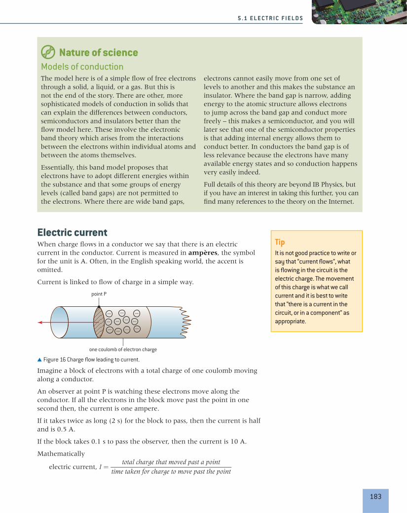
Electric currentWhen charge flows in a conductor we say that there is an electric current in the conductor. Current is measured in ampères, the symbol for the unit is A. Often, in the English speaking world, the accent is omitted.

Current is linked to flow of charge in a simple way.

one coulomb of electron charge

−−− − − −

−−

−−

−

point P

Figure 16 Charge flow leading to current.

Imagine a block of electrons with a total charge of one coulomb moving along a conductor.

An observer at point P is watching these electrons move along the conductor. If all the electrons in the block move past the point in one second then, the current is one ampere.

If it takes twice as long (2 s) for the block to pass, then the current is half and is 0.5 A.

If the block takes 0.1 s to pass the observer, then the current is 10 A.

Mathematically

electric current, I = total charge that moved past a point

____ time taken for charge to move past the point

TipIt is not good practice to write or say that “current flows”, what is flowing in the circuit is the electric charge. The movement of this charge is what we call current and it is best to write that “there is a current in the circuit, or in a component” as appropriate.

183


Worked examples1 In the shuttling ball experiment, the ball

moves between the two charged plates at a frequency of 0.67 Hz. The ball carries a charge of magnitude 72 nC each time it crosses from one plate to the other.

Calculate:

a) the average current in the circuit

b) the number of electrons transferred each time the ball touches one of the plates.

Solutiona) The time between the ball being at the same plate

= 1 __ f = 1

____ 0.67 = 1.5 s. The time to transfer 72 nC is therefore 0.75 s.

Current = 7.2 × 10–8

_______ 0.75 = 96 nA

b) The charge transferred is 72 nC = 7.2 ×10–8 C

Each electron has a charge of –1.6 × 10–19 C, so the number of electrons involved in the transfer is 7.2 × 10–8

________ 1.6 × 10–19 = 4.5 × 1011

2 a) Calculate the current in a wire through which a charge of 25 C passes in 1500 s.

b) The current in a wire is 36 mA. Calculate the charge that flows along the wire in one minute.

Solutiona) I = :Q

___ :t , so the current = 25

____ 1500 = 17 mA

b) :Q = I:t and ∆t = 60 s. Thus charge that flows = 3.6 × 10–2 × 60 = 2.2 C

Charge carrier drift speedTurn on a lighting circuit at home and the lamp lights almost immediately. Does this give us a clue to the speed at which the electrons in the wires move? In the Investigate! experiment on page 185, the stain indicating the position of the ions moves at no more than a few millimetres per second. The lower the value of the current, the slower the rate at which the ions move. This slow speed at which the ions move along the conductor is known as the drift speed.

We need a mathematical model to confirm this observation.

Nature of scienceAnother physics linkThis link between flowing charge and current is a crucial one. Electrical current is a macroscopic quantity, transfer of charge by electrons is a microscopic phenomenon in every sense of the word. This is another example of a link in physics between macroscopic observations and inferences about what is happening on the smallest scales.

It was the lack of knowledge of what happens inside conductors at the atomic scale that forced scientists, up to the end of the nineteenth century, to develop concepts such as current and field to explain the effects they observed. It also, as we shall see, led to a crucial mistake.

or in symbols

I = :Q

_ :t

The ampere is a fundamental unit defined as part of the SI. Although it is explained here in terms of the flow of charge, this is not how it is defined. The SI definition is based on ideas from magnetism and is covered in Sub-topics 1.1 and 5.4.

184


Investigate!

+−

potassium manganate(VII)crystal crocodile clip

microscope slidefilter paper soaked inaqueous ammonia solution

Figure 17

The speeds with which electrons move in a metal conductor during conduction are difficult to observe, but the progress of conducting ions in a liquid can be inferred by the trace they leave.

You should wear eye protection during this experiment.

Fold a piece of filter paper around a microscope slide and fix it with two crocodile clips at the ends of the slide. The crocodile

clips should be attached to leads that are connected to a low voltage power supply (no more than 25 V is required in this experiment).

Wet the filter paper with aqueous ammonia solution.

Take a small crystal of potassium manganate(VII) and place it in the centre of the filter paper. Ensure that the slide is horizontal.

Turn on the current and watch the crystal. You should see a stain on the paper moving away from the crystal.

Reverse the current direction to check that the effect is not due to the slide not being horizontal.

How fast is the stain moving?

Imagine a cylindrical conductor that is carrying an electric current I. The cross-sectional area of the conductor is A and it contains charge carriers each with charge q. We assume that each carrier has a speed v and that there are n charge carriers in 1 m3 of conductor – this quantity is known as the charge density.

cross-sectionalarea, A

n charge carriersper unit volume

length of volumeswept out in one second

v

− −− −

− −

− − −−

Pcharge carrier q

Figure 18 A model for conduction.

Figure 18 shows charge carriers, each of charge q, moving past point P at a speed v.

In one second, a volume Av of charge carriers passes P.

The total number of charge carriers in this volume is nAv and therefore the total charge in the volume is nAvq.

However, this is the charge that passes point P in one second, which is what we mean by the electric current. So

I = nAvq

185


The example shows that the drift speed of each charge is less than one-tenth of a millimetre each second. You may well be surprised by this result – but it is probably of the same order as the speed you observed in the experiment with the potassium manganate(VII). Although the electron charge is very small, the speed can also be small because there are very large numbers of free electrons available for conduction in the metal.

To see how sensitive the drift speed is to changes in the charge carrier density, we can compare the drift speed in copper with the drift speed in a semiconductor called germanium. The number of charge carriers in one cubic metre of germanium is about 109 less than in copper. So to sustain the same current in a germanium sample would require a drift speed 109 times greater than in the copper or a cross-sectional area 109 as large.

The slow drift speed in conductors for substantial currents poses the question of how a lamp can turn on when there may be a significant run of cable between switch and lamp. The charge carriers in the cable are drifting slowly around the cable. However, the information that the charge carriers are to begin to move when the switch is closed travels much more quickly – close to the speed of light in fact. The information is transferred when an electromagnetic wave propagates around the cable and produces a drift in all the free electrons virtually simultaneously. So the lamp can turn on almost instantaneously, even though, for direct current, it may take an individual electron many minutes or even hours to reach the lamp itself.

Potential differenceFree electrons move in a conductor when an electric field acts on the conductor. Later we shall see how devices such as electric cells and power supplies provide this electric field. At the same time the power supplies transfer energy to the electrons. As the electrons move through the conductors, they collide with the positive ions in the lattice and transfer the energy gained from the field to the ions.

In situations where fields act, physicists use two quantities called potential and potential difference when dealing with energy transfers. Potential difference (often abbreviated to “pd”) is a measure of the electrical potential energy transferred from an electron when it is moving between two points in a circuit. However, given the very small amount of charge possessed by each electron this amount of energy is also very small. It is better to use the much larger quantity represented by one coulomb of charge.

Worked example1 A copper wire of diameter 0.65 mm carries a

current of 0.25 A. There are 8.5 × 1028 charge carriers in each cubic metre of copper; the charge on each charge carrier (electron) is 1.6 × 10–19 C. Calculate the drift speed of the charge carriers.

SolutionRearranging the equation

v = I _ nAQ

and the area A of the wire is π ( 0.65 × 10–3

________ 2 ) 2 = 3.3 × 10–7 m2.

So v = 0.25 _________________________

8.5 × 1028 × 3.3 × 10–7 × 1.6 × 10–19

= 0.055 mm s–1

186


Potential difference between two points is defined as the work done (energy transferred) W when one unit of charge Q moves between the points.

potential difference = W _ Q

The symbol given to potential difference is V; its unit is the J C–1 and is named the volt (symbol: V) after the Italian scientist Alessandro Volta who was born in the middle of the eighteenth century and who worked on the development of electricity.

The potential difference between two points is one volt if one joule of energy is transferred per coulomb of charge passing between the two points.

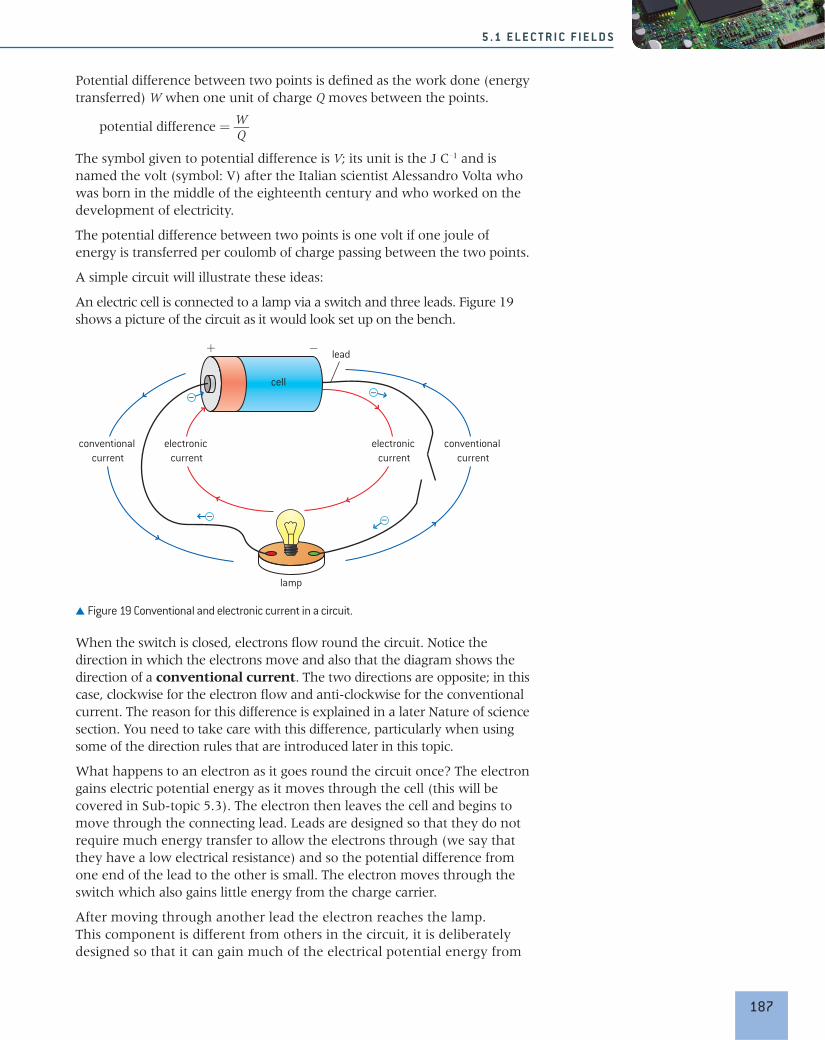
A simple circuit will illustrate these ideas:

An electric cell is connected to a lamp via a switch and three leads. Figure 19 shows a picture of the circuit as it would look set up on the bench.

electronic current

conventional current

lead

conventional current

electronic current

lamp

+ −

cell

Figure 19 Conventional and electronic current in a circuit.

When the switch is closed, electrons flow round the circuit. Notice the direction in which the electrons move and also that the diagram shows the direction of a conventional current. The two directions are opposite; in this case, clockwise for the electron flow and anti-clockwise for the conventional current. The reason for this difference is explained in a later Nature of science section. You need to take care with this difference, particularly when using some of the direction rules that are introduced later in this topic.

What happens to an electron as it goes round the circuit once? The electron gains electric potential energy as it moves through the cell (this will be covered in Sub-topic 5.3). The electron then leaves the cell and begins to move through the connecting lead. Leads are designed so that they do not require much energy transfer to allow the electrons through (we say that they have a low electrical resistance) and so the potential difference from one end of the lead to the other is small. The electron moves through the switch which also gains little energy from the charge carrier.

After moving through another lead the electron reaches the lamp. This component is different from others in the circuit, it is deliberately designed so that it can gain much of the electrical potential energy from

187


the electrons as they pass through it. The metal lattice in the filament gains energy and as a result the ions vibrate at greater speeds and with greater amplitudes. At these high temperatures the filament in the lamp will glow brightly; the lamp will be lit.

In potential difference terms, the pds across the leads and the switch are small because the passage of one coulomb of charge through them will not result in much energy transfer to the lattice. The pd across the lamp will be large because, for each coulomb going through it, large amounts of energy are transferred from electrons to the lattice ions in the filament raising its temperature.

Worked examples1 A high efficiency LED lamp is lit for 2 hours.

Calculate the energy transfer to the lamp when the pd across it is 240 V and the current in it is 50 mA.

Solution2 hours is 2 × 60 × 60 = 7200 s.

The charge transferred is I∆t = 7.2 × 103 × 50 × 10–3 = 360 C

Work done = charge × pd = 360 × 240 = 86 400 J

2 A cell has a terminal voltage of 1.5 V and can deliver a charge of 460 C before it becomes discharged.

a) Calculate the maximum energy the cell can deliver.

b) The current in the cell never exceeds 5 mA. Estimate the lifetime of the cell.

Solutiona) Potential difference,V = W __ q

so W = qV = 460 × 1.5 = 690 J

b) The current of 5 mA means that no more than 5 mC flows through the cell at any time. So 460

_____ 0.005 = 92 000 s (which is about 25 hours)

Nature of scienceConventional and electron currents In early studies of current electricity, the idea emerged that there was a flow of “electrical fluid” in wires and that this flow was responsible for the observed effects of electricity. At first the suggestion was that there were two types of fluid known as “vitreous” and “resinous”. Benjamin Franklin (the same man who helped draft the US Declaration of Independence) proposed that there was only one fluid but that it behaved differently depending on the circumstances. He was also the first scientist to use the terms “positive” and “negative”.

What then happened was that scientists assigned a positive charge to the “fluid” thought to be moving in the wires. This positive charge was said to flow out of the positive terminal of a power supply (because the charge was repelled) and went around the circuit re-entering the power

supply through the negative terminal. This is what we now term the conventional current.

In fact, we now know that in a metal the charge carriers are electrons and that they move in the opposite direction, leaving a power supply at the negative terminal. This is termed the electronic current. You should take care with these two currents and not confuse them.

You may ask: why do we now not simply drop the conventional current and talk only about the electronic current? The answer is that other rules in electricity and magnetism were set up on the assumption that charge carriers are positive. All these rules would need to be reversed to take account of our later knowledge. It is better to leave things as they are.

188


Electromotive force (emf)Another important term used in electric theory is electromotive force (usually written as “emf” for brevity). This term seems to imply that there is a force involved in the movement of charge, but the real meaning of emf is connected to the energy changes in the circuit. When charge flows electrical energy can go into another form such as internal energy (through the heating, or Joule, effect), or it can be converted from another form (for example, light (radiant energy) in solar (photovoltaic) cells). The term emf will be used in this course when energy is transferred to the electrons in, for example, a battery. (Other devices can also convert energy into an electrical form. Examples include microphones and dynamos.)

The term potential difference will be used when the energy is transferred from the electrical form. So, examples of this would be electrical into heat and light, or electrical into motion energy.

The table shows some of the devices that transfer electrical energy and it gives the term that is most appropriate to use for each one.

Device

converts energy from

into

pd or emf?Cell chemical electrical emfResistor electrical internal pdMicrophone sound electrical emfLoudspeaker electrical sound pdLamp electrical light (and

internal)pd

Photovoltaic cell light electrical emfDynamo kinetic electrical emfElectric motor electrical kinetic pd

Power, current, and pdWe can now answer the question of how much energy is delivered to a conductor by the electrons as they move through it.

Suppose there is a conductor with a potential difference V between its ends when a current I is in the conductor.

In time ∆t the charge Q that moves through the conductor is equal to I∆t.

The energy W transferred to the conductor from the electrons is QV which is (I∆t)V.

So the energy transferred in time ∆t is

W = IV∆t

The electrical power being supplied to the conductor is energy

_____ time = W __ ∆t and therefore

electrical power P = IV

Alternative forms of this expression that you will find useful are I = P __ V and V = P __ I

189


Nature of scienceA word about potentialThe use of the term “potential difference” implies that there is something called potential which can differ from point to point. This is indeed the case.

An isolated positive point charge will have field lines that radiate away from it. A small positive test charge in this field will have a force exerted on it in the field line direction and, if free to do so, will accelerate away from the original charge. When the test charge is close, there is energy stored in the system and we say that the system (the two charges interacting) has a high potential. When the test charge is further away, there is still energy stored, but it is smaller because the system has converted energy into the kinetic energy of the charge – it has “done work” on the charge. So to move the test charge away from the original charge transfers some of the original stored

energy; this is described as a loss of potential. Positive charges move from points of high potential to low potential if they are free to do so.

Negative charges on the other hand move from points of low potential to high. You can work this through yourself by imagining a negative test charge near a positive original charge. This time the two charges are attracted and to move the negative charge away we have to do work on the system. This increases the potential of the system. If charges are free they will fall towards each other losing potential energy. In what form does this energy re-appear?

We shall return to a discussion of potential in Topic 10. From now on Topic 5 only refers to potential differences.

The electronvoltEarlier we said that the energy possessed by individual electrons is very small. If a single electron is moved through a potential difference of equal to 15 V then as V = W __ Q , so W = QV and the energy gained by this electron is 15 × 1.6 ×10–19 J = 2.4 × 10–18 J. This is a very small amount and involves us in large negative powers of ten. It is more convenient to define a new energy unit called the electronvolt (symbol eV).

Worked examples1 A 3 V, 1.5 W filament lamp is connected to a

3 V battery. Calculate:

a) the current in the lamp

b) the energy transferred in 2400 s.

Solutiona) Electrical power, P = IV, so I = P __ V = 1.5

___ 3 = 0.5 A

b) The energy transferred every second is 1.5 J so in 2400 s, 3600 J.

2 An electric motor that is connected to a 12 V supply is able to raise a 0.10 kg load through

a distance of 1.5 m in 7 s. The motor is 40% efficient. Calculate the average current in the motor while the load is being raised.

SolutionThe energy gained is mg∆h = 0.01 × g ×1.5 = 0.147 J

The power output of the motor must be = 0.147

_____ 7 = 0.021 W

The current in the motor = P __ V = 0.021 _____ 12 = 1.8 mA.

Since the motor is 40% efficient the current will be 4.5 mA.

The unit of power is the watt (W) – 1 watt (1 W) is the power developed when 1 J is converted in 1 s, the same in both mechanics and electricity. So another way to think of the volt is as the power transferred per unit current in a conductor.

190


Worked examples1 An electron, initially at rest, is accelerated

through a potential difference of 180 V. Calculate, for the electron:

a) the gain in kinetic energy

b) the final speed.

Solution(a) The electron gains 180 eV of energy during its

acceleration.

1 eV ≡ 1.6 × 10–19 J so 180 eV ≡ 2.9 × 10–17 J

(b) The kinetic energy of the election = 1 __ 2 mv2 and the mass of the electron is 9.1 × 10–31 kg.

So v = √___

2Eke ___ me = √_________

2 × 2.9 × 10–17

___________ 9.1 × 10–31 = 8.0 × 106 m s–1.

2 In a nuclear accelerator a proton is accelerated from rest gaining an energy of 250 MeV. Estimate the final speed of the particle and comment on the result.

Solution The energy gained by the proton, in joules, is 4.0 × 10–11 J.

As before, v = √___

2Eke ___ mp = √_________

2 × 4.0 × 10–12

___________ 1.7 × 10–27 , but using a

value for the mass of the proton this time.

The numerical answer for v = 2.2 × 108 m s–1. This is a large speed, 70% of the speed of light. In fact the speed will be less than this as some of the energy goes into increasing the mass of the proton through relativistic effects rather than into the speed of the proton.

This is defined as the energy gained by an electron when it moves through a potential difference of one volt. An energy of 1 eV is equivalent to 1.6 × 10–19 J. The electronvolt is used extensively in nuclear and particle physics.

Be careful, although the unit sounds as though it might be connected to potential difference, like the joule it is a unit of energy.

191


Nature of sciencePeer review – a process in which scientists repeat and criticize the work of other scientists – is an important part of the modern scientific method. It was not always so. The work of Ohm was neglected in England at first as Barlow, a much-respected figure in his day, had published contradictory material to that of Ohm. In present-day science the need for repeatability in data collection is paramount. If experiments or other findings cannot be repeated, or if they contradict other scientists’ work, then a close look is paid to them before they are generally accepted.

Understanding Circuit diagrams Kirchhoff’s laws Heating effect of an electric current and its

consequences Resistance Ohm’s law Resistivity Power dissipation

5.2 Heating effect of an electric current

Applications and skills Drawing and interpreting circuit diagrams Indentifying ohmic and non-ohmic

conductors through a consideration of the V–I characteristic graph

Investigating combinations of resistors in parallel and series circuits

Describing ideal and non-ideal ammeters and voltmeters

Describing practical uses of potential divider circuits, including the advantages of a potential divider over a series variable resistor in controlling a simple circuit

Investigating one or more of the factors that affect resistivity

Solving problems involving current, charge, potential difference, Kirchhoff’s laws, power, resistance and resistivity

Equations resistance definition: R = V ___ I electrical power: P = VI = I2 R = V

2 _______ R

combining resistors: in series Rtotal = R1 + R2 + R3 ...

in parallel 1 ___________ Rtotal = 1 _______ R1

+ 1 _______ R2 + 1 _______ R3

+ ...

resisitivity definition: ρ = RA ________ l

Effects of electric current IntroductionThis is the first of three sub-topics that discusses some of the effects that occur when charge flows in a circuit. The three effects are:

heating effect, when energy is transferred to a resistor as internal energy

chemical effect, when chemicals react together to alter the energy of electrons and to cause them to move, or when electric current in a material causes chemical changes (Sub-topic 5.3)

magnetic effect, when a current produces a magnetic field, or when magnetic fields change near conductors and induce an emf in the conductor (Sub-topic 5.4).192


This sub-topic deals with the heating effect of a current after giving you some advice on setting up and drawing electric circuits.

Drawing and using circuit diagramsAt some stage in your study of electricity you need to learn how to construct electrical circuits to carry out practical tasks.

This section deals with drawing, interpreting, and using circuit diagrams and is designed to stand alone so that you can refer to it whenever you are working with diagrams and real circuits.

You may not have met all the components discussed here yet. They will be introduced as they are needed.

Circuit symbolsA set of agreed electrical symbols has been devised so that all physicists understand what is represented in a circuit diagram. The agreed symbols that are used in the IB Diploma Programme are shown in figure 1. Most of these are straightforward and obvious; some may be familiar to you already. Ensure that you can draw and identify all of them accurately.

resistor variable resistor

switch ammeter voltmeter

galvanometer

heating element fusepotentiometer

ac supplytransformer

battery lamp ac supply

joined wires wires crossing (not joined) cell

A V

diode variable power supplythermistor

capacitor

Figure 1 Circuit symbols.

193

5 . 2 H E A T I N G E F F E C T O F A N E L E C T R I C C U R R E N T

There are points to make about the symbols.

Some of the symbols here are intended for direct current (dc) circuits (cells and batteries, for example). Direct current refers to a circuit in which the charge flows in one direction. Typical examples of this in use would be a low-voltage flashlight or a mobile phone. Other types of electrical circuits use alternating current (ac) in which the current direction is first one way around the circuit and then the opposite. The time between changes is typically about 1/100th of a second. Common standards for the frequencies around the world include 50 Hz and 60 Hz. Alternating current is used in high-voltage devices (typically in the home and industry), where large amounts of energy transfer are required: kettles, washing machines, powerful electric motors, and so on. Alternating supplies can be easily transformed from one pd to another, whereas this is more difficult (though not impossible) for dc.

There are separate symbols for cells and batteries. Most people use these two terms interchangeably, but there is a difference: a battery is a collection of cells arranged positive terminal to negative – the diagram for the battery shows how they are connected. A cell only contains one source of emf. Sub-topic 5.3 goes into more detail about cells and batteries.

Circuit conventions It is not usual to write the name of the component in addition to giving

its symbol, unless there is some chance of ambiguity or the symbol is unusual. However, if the value of a particular component is important in the operation of the circuit it is usual to write its value alongside it.

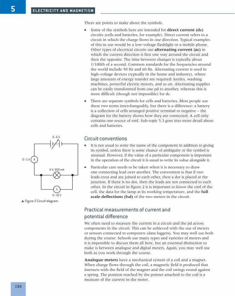
Particular care needs to be taken when it is necessary to draw one connecting lead over another. The convention is that if two leads cross and are joined to each other, then a dot is placed at the junction. If there is no dot, then the leads are not connected to each other. In the circuit in figure 2 it is important to know the emf of the cell, the data for the lamp at its working temperature, and the full scale deflections (fsd) of the two meters in the circuit.

Practical measurements of current and potential differenceWe often need to measure the current in a circuit and the pd across components in the circuit. This can be achieved with the use of meters or sensors connected to computers (data loggers). You may well use both during the course. Schools use many types and varieties of meters and it is impossible to discuss them all here, but an essential distinction to make is between analogue and digital meters. Again, you may well use both as you work through the course.

Analogue meters have a mechanical system of a coil and a magnet. When charge flows through the coil, a magnetic field is produced that interacts with the field of the magnet and the coil swings round against a spring. The position reached by the pointer attached to the coil is a measure of the current in the meter.

A

V

0–6 V

0–1 A

0–10 V

6 V, 300 mA

Figure 2 Circuit diagram.

194


Digital meters sample the potential difference across the terminals of the meter (or, for current, the pd across a known resistor inside the meter) and then convert the answer into a form suitable for display on the meter.

Ammeters measure the current in the circuit. As we want to know the size of the current in a component it is clear that the ammeter must have the same current. The ammeter needs to be in series with the circuit or component. An ideal ammeter will not take any energy from the electrons as they flow through it, otherwise it would disturb the circuit it is trying to measure. Figure 2 shows where the ammeter is placed to measure the current.

Voltmeters measure the energy converted per unit charge that flows in a component or components. You can think of a voltmeter as needing to compare the energy in the electrons before they enter a component to when they leave it, rather like the turnstiles (baffle gates) to a rail station that count the number of people (charges) going through as they give a set amount of money (energy) to the rail company. To do this the voltmeter must be placed across the terminals of the component or components whose pd is being measured. This arrangement is called parallel. Again, figure 2 shows this for the voltmeter.

Constructing practical circuits from a diagramWiring a circuit is an important skill for anyone studying physics. If you are careful and work in an organized way then you should have no problems with any circuit no matter how complex.

As an example, this is how you might set up one of the more difficult circuits in this course.

A

V

(a)

step 1

step 2

step 3

step 4

A B

A

B'A'

link A → A'; B → B'

(c)

V

Figure 3 Variable resistors.

(b)

195


This is a potential divider circuit that it is used to vary the pd across a component, in this case a lamp.

The most awkward component to use here is the potential divider itself (a form of variable resistor, that is sometimes known as a potentiometer). In one form it has three terminals (figure 3(b)), in another type it has three in a rotary format. The three-terminal linear device has a terminal at one end of a rod with a wiper that touches the resistance windings, and another two terminals one at each end of the resistance winding itself.

Begin by looking carefully at the diagram figure 3(a). Notice that it is really two smaller circuits that are linked together: the top sub-circuit with the cell, and the bottom sub-circuit with the lamp and the two meters. The bottom circuit itself consists of two parts: the lamp/ammeter link together with the voltmeter loop.

The rules for setting up a circuit like this are:

If you do not already have one, draw a circuit diagram. Get your teacher to check it if you are not sure that it is correct.

Before starting to plug leads in, lay out the circuit components on the bench in the same position as they appear on the diagram.

Connect up one loop of the circuit at a time.

Ensure that components are set to give minimum or zero current when the circuit is switched on.

Do not switch the circuit on until you have checked everything.

Figure 3(c) shows a sequence for setting up the circuit step-by-step.

Another skill you will need is that of troubleshooting circuits – this is an art in itself and comes with experience. A possible sequence is:

Check the circuit – is it really set up as in your diagram?

Check the power supply (try it with another single component such as a lamp that you know is working properly).

Check that all the leads are correctly inserted and that there are no loose wires inside the connectors.

Check that the individual components are working by substituting them into an alternative circuit known to be working.

Resistance We saw in Sub-topic 5.1 that, as electrons move through a metal, they interact with the positive ions and transfer energy to them. This energy appears as kinetic energy of the lattice, in other words, as internal energy: the metal wire carrying the current heats up.

However, simple comparison between different conductors shows that the amount of energy transferred can vary greatly from metal to metal. When there is the same current in wires of similar size made of tungsten or copper, the tungsten wire will heat up more than the

196


copper. We need to take account of the fact that some conductors can achieve the energy transfer better than others. The concept of electrical resistance is used for this.

The resistance of a component is defined as

potential difference across the component

____ current in the component

The symbol for resistance is R and the definition leads to a well-known equation

R = V _ I

The unit of resistance is the ohm (symbol Ω; named after Georg Simon Ohm, a German physicist). In terms of its fundamental units, 1 Ω is 1 kg m2 s–3 A–2; using the ohm as a unit is much more convenient!

Alternative forms of the equation are: V = IR and I = V __ R

Investigate!Resistance of a metal wire

Take a piece of metal wire (an alloy called constantan is a good one to choose) and

connect it in the circuit shown. Use a power supply with a variable output so that you can alter the pd across the wire easily.

If your wire is long, coil it around an insulator (perhaps a pencil) and ensure that the coils do not touch.

Take readings of the current in the wire and the pd across it for a range of currents. Your teacher will tell you an appropriate range to use to avoid changing the temperature of the wire.

For each pair of readings divide the pd by the current to obtain the resistance of the wire in ohms.

A

V

Figure 4

A table of results is shown in figure 5 for a metal wire 1 m in length with a diameter of 0.50 mm. For each pair of readings the resistance of the wire has been calculated by dividing the pd by the current. Although the resistance values are not identical (it is an experiment with real errors, after all), they do give an average value for the resistance of 2.54 Ω. This should be rounded to 2.5 Ω given the signficant figures in the data.

current/A pd/V0.130.260.500.761.011.271.531.78

2.552.602.502.532.532.542.552.54

0.050.100.200.300.400.500.600.70

resistance/E

Figure 5 Variation of pd with current for a conductor.

197


Nature of scienceEdison and his lampThe conversion of electrical energy into internal energy was one of the first uses of distributed electricity. Thomas Edison an inventor and entrepreneur, who worked in the US at around the end of the nineteenth century, was a pioneer of electric lighting. The earliest forms of light were provided by producing a current in a metal or carbon filament. These filaments heated up

until they glowed. Early lamps were primitive but produced a revolution in the way that homes and public spaces were lit. The development continues today as inventors and manufacturers strive to find more and more efficient electric lamps such as the light-emitting diodes (LED). More developments will undoubtedly occur during the lifetime of this book.

Worked exampleThe current in a component is 5.0 mA when the pd across it is 6.0 V.

Calculate:

a) the resistance of the component

b) the pd across the component when the current in it is 150 µA.

Solutiona) R = V __ I = 6

______ 5 × 10–3 = 1.2 kΩ

b) V = IR = 1.5 × 10–4 × 1.2 × 103 = 0.18 A

Ohm’s lawFigure 6 shows the results from the metal wire when they are plotted as a graph of V against I.

1.00

1.20

1.40

1.60

1.80

2.00

0.80

0.60

0.40

0.20

0.00

pd/V

current/A0.100.00 0.20 0.30 0.40 0.50 0.60 0.70 0.80

Figure 6 pd against current from the table.

A best straight line has been drawn through the data points. For this wire, the resistance is the same for all values of current measured. Such a resistor is known as ohmic. An equivalent way to say this is that the potential difference and the current are proportional (the line is straight and goes through the origin). In the experiment carried out to obtain these data, the temperature of the wire did not change.

This behaviour of metallic wires was first observed by Georg Simon Ohm in 1826. It leads to a rule known as Ohm’s law.

Ohm’s law states that the potential difference across a metallic conductor is directly proportional to the current in the conductor providing that the physical conditions of the conductor do not change.

By physical conditions we mean the temperature (the most important factor as we shall see) and all other factors about the wire. But the temperature factor is so important that the law is sometimes stated replacing the term “physical conditions” with the word “temperature”.

198


Investigate!Variation of resistance of a lamp filament

Use the circuit you used in the investigation on resistance of a metal wire, but repeat the experiment with a filament lamp instead of the wire.

Your teacher will advise you of the range of currents and pds to use.

This time do the experiment twice, the second time with the charge flowing through the lamp in the opposite direction to the first. There are

two ways to achieve this: the first is to reverse the connections to the power supply, also reversing the connections to the ammeter and voltmeter (if the meters are analogue). The second way is somewhat easier, simply reverse the lamp and call all the readings negative because they are in the opposite direction through the lamp.

Plot a graph of V (y-axis) against I (x-axis) with the origin (0,0) in the centre of the paper. Figure 7 shows an example of a V–I graph for a lamp.

4

2

20−20−40−60 40 600

0

−2

−4

−6

6pd/V

current, I/mA

Figure 7

Nature of scienceOhm and BarlowOhm’s law has its limitations because it only tells us about a material when the physical conditions do not change. However, it was a remarkable piece of work that did not find immediate favour. Barlow was an English scientist who was held in high respect for his earlier work and had recently published an alternative theory on conduction. People simply did not believe that Barlow could be wrong.

This immediate acceptance of one scientist’s work over another would not necessarily happen today. Scientists use a system of peer review. Work published by one scientist or scientific group must be set out in such a way that other scientists can repeat the experiments or collect the same data to check that there are no errors in the original work. Only if the scientific community as a whole can verify the data is the new work accepted as scientific “fact”.

Towards the end of the 20th century a research group thought that it had found evidence that nuclear fusion could occur at low temperatures (so-called “cold fusion”). Repeated attempts by other research groups to replicate the original results failed, and the cold fusion ideas were discarded.

199


TOK

But is it a law?

This rule of Ohm is always called a law – but is it? In reality it is an experimental description of how a group of materials behave under rather restricted conditions. Does that make it a law? You decide.

There is also another aspect to the law that is often misunderstood.

Our definition of resistance is that R = V ___ I or V = IR. Ohm’s law states that

V ∝ I

and, including the constant of proportionality k,

V = kI

We therefore define R to be the same as k, but the definition of resistance does not correspond to Ohm’s law (which talks only about a proportionality). V = IR is emphatically not a statement of Ohm’s law and if you write this in an examination as a statement of the law you will lose marks.

The graph is not straight (although it goes through the origin) so V and I are not proportional to each other. The lamp does not obey Ohm’s law and it is said to be non-ohmic. However, this is not a fair test of ohmic behaviour because the filament is not held at a constant temperature. If it were then, as a metal, it would probably obey the law.

When the resistance is calculated for some of the data points it is not constant either. The table shows the resistance values at each of the positive current points.

Current/mA Resistance/Ω20 5034 5941 7347 8552 9655 109

The data show that resistance of the lamp increases as the current increases. At large currents, it takes greater changes in pd to change the current by a fixed amount. This is exactly what you might have predicted. As the current increases, more energy is transferred from the electrons every second because more electrons flow at higher currents. The energy goes into increasing the kinetic energy of the lattice ions and therefore the temperature of the bulk material. But the more the ions vibrate in the lattice, the more the electrons can collide with them so at higher temperatures even more energy is transferred to the lattice by the moving charges.

Other non-ohmic conductors include semiconducting diodes and thermistors; these are devices made from a group of materials known as semiconductors.

Investigate!Diodes and thermistors

You can easily extend the Investigate! lamp experiment to include these two types of device. There are some extra practical points however:

The diode will require a protecting resistor in series with it (100 Ω is usually appropriate) as the current can become very large at even quite small potential differences; this will cause the diode to melt as large amounts of energy are transferred to it. The resistor limits the current so that the diode is not damaged.

The thermistor also needs care, because as it heats up its resistance decreases and if too much current is used, the thermistor can also be destroyed.

TipNotice that these resistances were calculated for each individual data point using V __ I . They were not evaluated from the tangent to the graph at the current concerned. The definition of resistance is in terms of V __ I not in terms of ∆V

___ ∆I which

is what the tangent would give.

200


The results of these experiments and some others are summarized in the I–V graphs in figure 8.

I

V

ohmic conductor

00

I

V

filament lamp

00

00

00

II

neon tubeV

thermistorV

I

V

semiconducting diode

00

Figure 8 I–V graphs for various conductors.

Semiconducting diodesSemiconducting diodes are designed only to allow charges to flow through them in one direction. This is seen clearly in the graph. For negative values of V there is actually a very small current flowing in the negative direction but it is far less than the forward current. The nature of semiconductor material also means that there is no significant current in the forward direction until a certain forward pd is exceeded.

ThermistorsThermistors are made from one of the two elements that are electrical semiconductors: silicon and germanium. There are several types of thermistor, but we will only consider the negative temperature coefficient type (ntc). As the temperature of an ntc thermistor increases, its resistance falls. This is the opposite behaviour to that of a metal.

Semiconductors have many fewer free electrons per cubic metre compared with metals. Their resistances are typically 105 times greater than similar samples of metals. However, unlike in a metal, the charge density in semiconductors depends strongly on the temperature. The higher the temperature of the semiconductor, the more charge carriers are made available in the material.

As the temperature rises in the germanium:

The lattice ions vibrate more and impede the movement of the charge carriers. This is exactly the same as in metals and also leads to an increase in resistance.

More and more charge carriers become available to conduct because the increase in temperature provides them with enough energy to break away from their atoms. This leads to a large decrease in resistance.

The second effect is much greater than the first and so the net effect is that conduction increases (resistance falls) as the temperature of the semiconductor rises.

201


Investigate!How resistance depends on size and shape

You will need a set of wires made from the same metal or metal alloy. The wires should have a circular cross-section and be available in a range of different diameters. You will also need to devise a way to vary the length of one of the wires in the circuit.

Use the circuit in figure 4 on p197 to answer the following questions:

How does the resistance R of one of the wires vary with length l?

How does the resistance R of the wires vary with diameter d when the wires all have the same length?

Try to make things easy for your analysis. Double and halve the values of length to see what difference this makes to the resistance – is there an obvious relationship? The diameter of the wire may be more difficult to test in this way, but a graph of resistance against diameter may give you a clue.

Once you have an idea what is going on, you may decide that the best way to answer these questions is to plot graphs of

R against l, and

R against 1 __ d2

ResistivityThe resistance of a sample of a material depends not only on what it is made of, but also on the physical dimensions (the size and shape) of the sample itself.

The graphs suggested in the Investigate! should give straight lines that go through the origin and can be summed up in the following rule.

The resistance of a conductor is:

proportional to its length l

inversely proportional to its cross-sectional area A (which is itself proportional to d2).

So

R ∝ l _ A

This leads to a definition of a new quantity called resistivity.

Resistivity ρ is defined by

ρ = RA _ l

The unit of resistivity is the ohm-metre (symbol Ω m). Take care here: this is ohm metre. It is not ohm metre–1 – a mistake frequently made by students in examinations. The meaning of ohm metre–1 is the resistance of one metre length of a particular conductor, which is a relevant quantity to know, but is not the same as resistivity.

Resistivity is a quantity of considerable use. The resistance of a material depends on the shape of the sample as well as what it is made from. Even a constant volume of a material will have values of resistance that depend on the shape. However, the value of the resistivity is the same for all samples of the material. Resistivity is independent of shape or size just like quantities such as density (where the size of a material has been

202


removed by the use of volume) or specific latent heat (where the value is related to unit mass of the material).

Worked examples1 A uniform wire has a radius of 0.16 mm and a

length of 7.5 m. Calculate the resistance of the wire if its resistivity is 7.0 × 10–7 Ω m.

SolutionUnless told otherwise, assume that the wire has a circular cross-section.

area of wire = π(1.6 × 10–4)2 = 8.04 × 10–8 m2

ρ = RA _ l

and R = ρl

_ A

= 7.0 × 10–7 × 7.5 __ 8.04 × 10–8

= 65 Ω

2 Calculate the resistance of a block of copper that has a length of 0.012 m with a width of 0.75 mm and a thickness of 12 mm. The resistivity of copper is 1.7 × 10–8 Ω m.

SolutionThe cross-sectional area of the block is 7.5 × 10–4 × 1.2 × 10–2 = 9.0 × 10–6 m2

The relevant dimension for the length is 0.012 m, so

R = ρl

_ A

= 1.7 × 10–8 × 0.012 _____________

9.0 × 10–6 = 0.023 mΩ

Investigate!Resistivity of pencil lead

pencil

V

A

Figure 9

Graphite is a semi-metallic conductor and is a constituent of the lead in a pencil. Another constituent in the pencil lead is clay. It is the ratio of graphite to clay that determines the “hardness” of the pencil. This experiment enables you to estimate the resistivity of the graphite.

Take a B grade pencil (sometimes known as #1 grade in the US) and remove about 1.5 cm of the wood from each end leaving a cylinder of the lead exposed. Attach a crocodile (alligator) clip firmly to each end. Use leads attached to the crocodile clips to connect the pencil into a circuit in order to measure the resistance of the lead. Expect the resistance of the pencil lead to be about 1 Ω for the purpose of choosing the power supply and meters.

Determine the resistance of the lead.

Measure the length of pencil lead between the crocodile clips.

Measure the diameter of the lead using a micrometer screw gauge or digital callipers and calculate the area of the lead.

Using the data, calculate the resistivity of the lead. The accepted value of the resistivity of graphite is about 3 × 10–5 Ω m but you will not expect to get this value given the presence of clay in the lead as well.

Take the experiment one step further with a challenge. Use your pencil to uniformly shade a 10 cm by 2 cm area on a piece of graph paper. This will make a graphite resistance film on the paper. Attach the graphite film to a suitable circuit and measure the resistance of the film. Knowing the resistance and the dimensions of your shaded area should enable you to work out how thick the film is. (Hint: in the resistivity equation, the length is the distance across the film, and the area is width of the film × thickness of the film.)

203


Practical resistors Resistors are of great importance in the electronics and electrical industries. They can be single value (fixed) devices or they can be variable. They can be manufactured in bulk and are readily and cheaply available.

Resistors come in different sizes. Small resistors can have a large resistance but only be able to dissipate (lose) a modest amount of energy every second. If the power that is being generated in the resistor is too large, then its temperature will increase and in a worst case, it could become a thermal fuse! Resistors are rated by their manufacturers so that, for example, a resistor could have a resistance of 270 Ω with a power rating of 0.5 W. This would mean that the maximum current that the resistor can safely carry is √___

0.5 ___ 270 = 43 mA.

Combining resistorsElectrical components can be linked together in two ways in an electrical circuit: in series, where the components are joined one after another as the ammeter, the cell and the resistor in figure 10, or in parallel as are the resistor and the voltmeter in the same figure.

Two components connected in series have the same current in each. The number of free electrons leaving the first component must equal the number entering the second component; if electrons were to stay in the first component then it would become negatively charged and would repel further electrons and prevent them from entering it. The flow of charges would rapidly grind to a halt. This is an important rule to understand.

In series the potential differences (pds) add. To see this, think of charge as it travels through two components, the total energy lost is equal to the sum of the two separate amounts of energy in the components. Because the charge is the same in both cases, therefore, the sum of the pds is equal to the total pd dropped across them.

Components in parallel, on the other hand, have the same pd across them, but the currents in the components differ when the resistances of the components differ. Consider two resistors of different resistance values, in parallel with each other and connected to a cell. If one of the resistors is temporarily disconnected then the current in the remaining resistor is given by the emf of the cell divided by the resistance. This will also be true for the other resistor if it is connected alone. If both resistors are now connected in parallel with each other, both resistors have the same pd across them because a terminal of each resistor is connected to one of the terminals of the cell. The cell will have to supply more current than if either resistor were there alone – to be precise, it has to supply the sum of the separate currents.

To sum up

Currents ... Potential differences ...

In series ...are the same ...addIn parallel ...add ...are the same

A

V

Figure 10

204


Investigate!Resistors in series and parallel

For this experiment you need six resistors, each one with a tolerance of ±5%. Two of these resistors should be the same. The tolerance figure means that the manufacturer only guarantees the value to be within 5% of the nominal value – “nominal” means the printed value. Your resistors may have the nominal value written on them or you may have to use the colour code printed on them. The code is easy to decipher.

silvergoldblackbrownred 2orangeyellowgreenblueviolet

0.01

2

multiplier tolerance

0.11

10100

1 k10 k

100 k

10%5%

1%2%

0.5%1 M

10 Mgreywhite

01

3456789

7 ×1k (±5%) = 27kΩ (±5%)

You also need a multimeter set to measure resistance directly and a way to join the resistors together and to connect them to the multimeter.

First, measure the resistance of each resistor and record this in a table.

Take the two resistors that have the same nominal value and connect them in series. Measure the resistance of the combination. Can you see a rule straight away for the combined resistance of two resistors?

Repeat with five of the possible combinations for connecting resistors in series.

Now measure the combined resistance of the two resistors with the same nominal value when they are in parallel. Is there an obvious rule this time?

One way to express the rule for combining

two resistors R1 and R2 in parallel is as R1 R2 ______ R1 + R2

.

Test this relationship for five combinations of parallel resistors.

Test your two rules together by forming combinations of three resistors such as:

These ideas provide a set of rules for the combination of resistors in various arrangements:

Resistors in seriesSuppose that there are three resistors in series: R1, R2 and R3 (figure 11(a)). What is the resistance of the single resistor that could replace them so that the resistance of the single resistor is equivalent to the combination of three?

The resistors are in series (figure 11(a)) and therefore the current I is the same in each resistor.

Using the definition of resistance, the pd across each resistor, V1, V2 and V3 is

V1 = IR1 V2 = IR2 and V3 = IR3

205


The single resistor with a resistance R has to be indistinguishable from the three in series. In other words, when the current through this single resistor is the same as that through the three, then it must have a pd V across it such that

V = IR

I

I

R2

R2

R3

R3

R1

(a) series

R1

V1

I1

I2

I3

V2

V

(b) parallelV

V3

Figure 11 Resistors in series and parallel.

As this is a series combination, the potential differences add, so

V = V1 + V2 + V3

Therefore

IR = IR1 + IR2 + IR3

and cancelling I leads to, in series

R = R1 + R2 + R3

When resistors are combined in series, the resistances add to give the total resistance.

Resistors in parallelThree resistors in parallel (figure 11(b)) have the same pd V across them (figure 11(b)). The currents in the three separate resistors add to give the current in the connecting leads to and from all three resistors, therefore

I = I1 + I2 + I3

Each current can be written in terms of V and R using the definition of resistance:

V _ R

= V _ R1

+ V _ R2

+ V _ R3

206


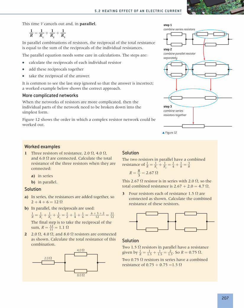
This time V cancels out and, in parallel,

1 _ R

= 1 _ R1

+ 1 _ R2

+ 1 _ R3

In parallel combinations of resistors, the reciprocal of the total resistance is equal to the sum of the reciprocals of the individual resistances.

The parallel equation needs some care in calculations. The steps are:

calculate the reciprocals of each individual resistor

add these reciprocals together

take the reciprocal of the answer.

It is common to see the last step ignored so that the answer is incorrect; a worked example below shows the correct approach.

More complicated networksWhen the networks of resistors are more complicated, then the individual parts of the network need to be broken down into the simplest form.

Figure 12 shows the order in which a complex resistor network could be worked out.

Worked examples1 Three resistors of resistance, 2.0 Ω, 4.0 Ω,

and 6.0 Ω are connected. Calculate the total resistance of the three resistors when they are connected:

a) in series

b) in parallel.

Solution a) In series, the resistances are added together, so

2 + 4 + 6 = 12 Ωb) In parallel, the reciprocals are used:

1 __ R = 1 __ R1

+ 1 __ R2

+ 1 __ R3

= 1 __ 2 + 1 __ 4 + 1 __ 6 = 6 + 3 + 2 ________ 12 = 11

__ 12

The final step is to take the reciprocal of the sum, R = 12

__ 11 = 1.1 Ω2 2.0 Ω, 4.0 Ω, and 8.0 Ω resistors are connected

as shown. Calculate the total resistance of this combination.

2.0 E4.0 E

8.0 E

SolutionThe two resistors in parallel have a combined resistance of 1 __ R = 1 __ R1

+ 1 __ R2

= 1 __ 4 + 1 __ 8 = 3 __ 8

R = 8 _ 3

= 2.67 ΩThis 2.67 Ω resistor is in series with 2.0 Ω, so the total combined resistance is 2.67 + 2.0 = 4.7 Ω.

3 Four resistors each of resistance 1.5 Ω are connected as shown. Calculate the combined resistance of these resistors.

SolutionTwo 1.5 Ω resistors in parallel have a resistance given by 1 __ R = 1

___ 1.5 + 1 ___ 1.5 = 2

___ 1.5 . So R = 0.75 Ω.

Two 0.75 Ω resistors in series have a combined resistance of 0.75 + 0.75 =1.5 Ω

step 1combine series resistors

step 2combine parallel resistorseparately

step 3combine series resistors together

Figure 12

207


Potential dividerIn the section on circuit diagrams, a potential divider circuit was shown. This is a circuit commonly used with sensors and also to produce variable potential differences. It has some advantages over the simpler variable resistor circuit even though it is more complicated to set up.

R1 Rtop

thermistor

V1

V2R2 Vout Vout

Vin

V

(a) (b) (c)

Vin

R

LDR

Vin

Figure 13 The potential divider.

The most basic potential divider consists of two resistors with resistances R1 and R2 in series with a power supply. This arrangement is used to provide a fixed pd at a value somewhere between zero and the emf of the power supply. Figure 13(a) shows the arrangement.

The two resistors have the same current in them, and the sum of the pds across the resistors is equal to the source emf.

So

The current I in both resistors is

I = total pd across both resistors

___ total resistance

= V _ R

As usual,

V1 = IR1 and V2 = IR2

The resistors are in series so

R = R1 + R2

This leads to equations for the pd across each resistor

V1 = R1 _

( R1 + R2 ) Vin and V2 = R2 _

( R1 + R2 ) Vin

Using a potential divider with sensors It is a simple matter to extend the fixed pd arrangement to a circuit that will respond to changes in the external conditions. Such an arrangement might be used by a computer that can sense changes in pd and respond accordingly, for example, by turning on a warning siren if a refrigerator becomes too warm, or turning on a light when it becomes dark.

Typical circuits are shown in figures 13(b) and13(c).

In figure 13(b) a thermistor is used instead of one of the fixed resistors.

Worked example1 A potential divider

consists of two resistors in series with a battery of 18 V. The resistors have resistances 3.0 Ω and 6.0 Ω. Calculate, for each resistor:

a) the pd across it

b) the current in it.

Solution a) The pd across the 3.0 Ω

resistors Vin × R1 _______ (R1 + R2)

= 18 × 3 _____ 3 + 6

= 6.0 V. The pd across the 6.0 Ω is then 18 – 6.0 V = 12 V.

b) The current is the same in both resistors because they are in series. The total resistance is 9.0 Ω and the emf of the battery is 18 V. The current = V __ R = 18

__ 9 = 2.0 A.

208


Recall that when a thermistor is at a high temperature its resistance is small, and that the resistance increases when the temperature falls.

Rather than calculating the values, for this example we will use our knowledge of how pd and current are related to work out the behaviour of the circuit from first principles.

Suppose the temperature is low and that the thermistor resistance is high relative to that of the fixed-value resistor. Most of the pd will be dropped across the thermistor and very little across the fixed resistor. If you cannot see this straight away, remember the equations from the previous section:

Vthermistor = VinRthermistor __

( Rthermistor + Rresistor ) and Vresistor = VinRresistor __

( Rthermistor + Rresistor )

If Rthermistor ⪢ Rresistor (⪢ means “much greater than”) then Rthermistor ≈ (Rthermistor + Rresistor) and Vthermistor ≈ Vin.

So the larger resistance (the thermistor at low temperatures) has the larger pd across it.

If the thermistor temperature now increases, then the thermistor resistance will fall. Now the fixed-value resistor will have the larger resistance and the pds will be reversed with the thermistor having the small voltage drop across it. A voltage sensor connected to a computer can be set to detect this voltage change and can activate an alarm if the thermistor has too high a temperature.

You may be asking what the resistance of the fixed resistor should be. The answer is that it is normally set equal to that of the thermistor when it is at its optimum (average) temperature. Then any deviation from the average will change the potential difference and trigger the appropriate change in the sensing circuit.

The same principle can be applied to another sensor device, a light-dependent resistor (LDR). This, like the thermistor, is made of semiconducting material but this time it is sensitive to photons incident on it. When the light intensity is large, charge carriers are released in the LDR and thus the resistance falls. When the intensity is low, the resistance is high as the charge carriers now re-combine with their atoms.

Look at figure 13(c). You should be able to explain that when the LDR is in bright conditions then the pd across the fixed resistor is high.

Using a potential divider to give a variable pdA variable resistor circuit is shown in figure 14(a). It consists of a power supply, an ammeter, a variable resistor and a resistor. The value of each component is given on the diagram.

We can predict the way this circuit will behave.

When the variable resistor is set to its minimum value, 0 Ω, then there will be a pd of 2 V across the resistor and a current of 0.2 A in the circuit.

When the variable resistor is set to its maximum value, 10 Ω, then the total resistance in the circuit is 20 Ω, and the current is 0.1 A.

This means that with 0.1 A in the 10 Ω fixed resistor, only 1 V is dropped across it. Therefore the range of pd across the fixed resistor can only vary

209


from 1 V to 2 V – half of the available pd that the power supply can in principle provide. You should now be able to predict the range across the variable resistor.

2 V

0 V

1 V

A

V

fixed resistor10 E

variable resistor0–10 E

2 V

fixed resistor10 E

slider

(a) variable resistor (b) potential divider

2 V

Figure 14

The limited range is a significant limitation in the use of the variable resistor. To achieve a better range, we could use a variable resistor with a much higher range of resistance. To get a pd of 0.1 V across the fixed resistor the resistance of the variable resistor has to be about 200 Ω. If the fixed resistor had a much greater resistance, then the variable resistor would need an even higher value too and this would limit the current.

The potential divider arrangement (figure 14(b)) allows a much greater range of pd to the component under test than does a variable resistor in series with the component. In a potential divider, the same variable resistor can be used but the set up is different and involves the use of the three terminals on the variable resistor. (A variable resistor is also sometimes called a rheostat.) One terminal is connected to one side of the cell, and the other end of the rheostat resistor is connected to the other terminal of the cell.

The potential at any point along the resistance winding depends on the position of the slider (or wiper) that can be swept across the windings from one end to the other. Typical values for the potentials at various points on the windings are shown for the three blue slider positions on figure 14(b). The component that is under test (again, a resistor in this case) is connected in a secondary circuit between one terminal of the resistance winding and the slider on the rheostat. When the slider is positioned at one end, the full 2 V from the cell is available to the resistor under test. When at the other end, the pd between the ends of the resistor is 0 V (the two leads to the resistor are effectively connected directly to each other at the variable resistor).

You should know how to set this arrangement up and also how to draw the circuit and explain its use.

210


Heating effect equationsWe saw earlier that the power P dissipated in a component is related to the pd V across the component and the current I in it:

P = IV

The energy E converted in time ∆t is

E = IV∆t

When either V or I are unknown, then two more equations become available:

P = IV = I2R = V2 _

R

Investigate!Variable resistor or potential divider?

Set up the two circuits shown in figure 14. Match the value of the fixed resistor to the variable resistor – they do not need to be exactly the same but should be reasonably close. Add a voltmeter connected across the fixed resistor to check the pd that is available across it.

Make sure that the maximum current rating for the fixed resistor and the variable resistor cannot be exceeded.

Check the pd available in the two cases and convince yourself that the potential divider gives a wider range of voltages.

Worked examples1 A light sensor consists of a 6.0 V battery, a

1800 Ω resistor and a light-dependent resistor in series. When the LDR is in darkness the pd across the resistor is 1.2 V.

a) Calculate the resistance of the LDR when it is in darkness.

b) When the sensor is in the light, its resistance falls to 2400 Ω. Calculate the pd across the LDR.

Solutiona) As the pd across the resistor is 1.2 V, the pd

across the LDR must be 6 – 1.2 = 4.8 V.

The current in the circuit is I = V __ R = 1.2

____ 1800 = 0.67 mA. The resistance of the LDR is V __ I = 4.8

________ 0.67 × 10–3 = 7200 Ω.

b) The ratio of resistance across LDR ________________

resistance across 1800 Ω = 2400 ____ 1800 = 1.33.

This is the same value as pd across LDR

___________ pd across 1800 Ω . For the

ratio of pds to be 1.33, the pds must be 2.6 V

and 3.4 V with the 3.4 V across the LDR.

2 A thermistor is connected in series with a fixed resistor and a battery. Describe and explain how the pd across the thermistor varies with temperature.

Solution As the temperature of the thermistor rises, its resistance falls. The ratio of the pd across the fixed resistor to the pd across the thermistor rises too because the thermistor resistance is dropping. As the pd across the fixed resistor and thermistor is constant, the pd across the thermistor must fall.

The change in resistance in the thermistor occurs because more charge carriers are released as the temperature rises. Even though the movement of the charge carriers is impeded at higher temperatures, the release of extra carriers means that the resistance of the material decreases.

211


Worked examples1 Calculate the power dissipated in a 250 Ω resistor when the pd

across it is 10 V.

SolutionP = V

2 _

R = 102

_ 250

= 0.40 W

2 A 9.0 kW electrical heater for a shower is designed for use on a 250 V mains supply. Calculate the current in the heater.

Solution P = IV so I = P _

V = 9000 _

250 = 36 A

3 Calculate the resistance of the heating element in a 2.0 kW electric heater that is designed for a 110 V mains supply.

SolutionP = V

2 _

R ; R = V

2 _

P = 1102

_ 2000

= 6.1 A.

Kirchhoff’s first and second lawsThis section contains no new physics, but it will consolidate your knowledge and put the electrical theory you have learnt so far into a wider physical context.

We saw that the charge carriers in a conductor move into and out of the conductor at equal rates. If 106 flow into a conductor in one second, then 106 must flow out during the same time to avoid the buildup of a static charge.

We also considered what happens when current splits into two or more parts at the junction where a parallel circuit begins. This can be taken one step further to a situation where there is more than one incoming current at the junction too.

Figure 15 shows a junction with three incoming currents and two outgoing ones. Our rule about the incoming charge equating to the outgoing charge must apply here too, so algebraically:

I1 + I2 + I3 = I4 + I5

A general way to write this is to use the ∑ sign (meaning “add up everything”), so that

for any junction ∑I = 0

When using the ∑ notation, remember to get the signs of the currents correct. Call any current in positive, and any current out negative.

Figure 15 Kirchhoff’s first law.

I2

I5

I1

I4

I3

and

E = IV∆t = I2R∆t = V 2 _ R

∆t

These equations will allow you to calculate the energy converted in electrical heaters and lamps and so on. Applications that you may come across include heating calculations, and determining the consumption of energy in domestic and industrial situations.

212


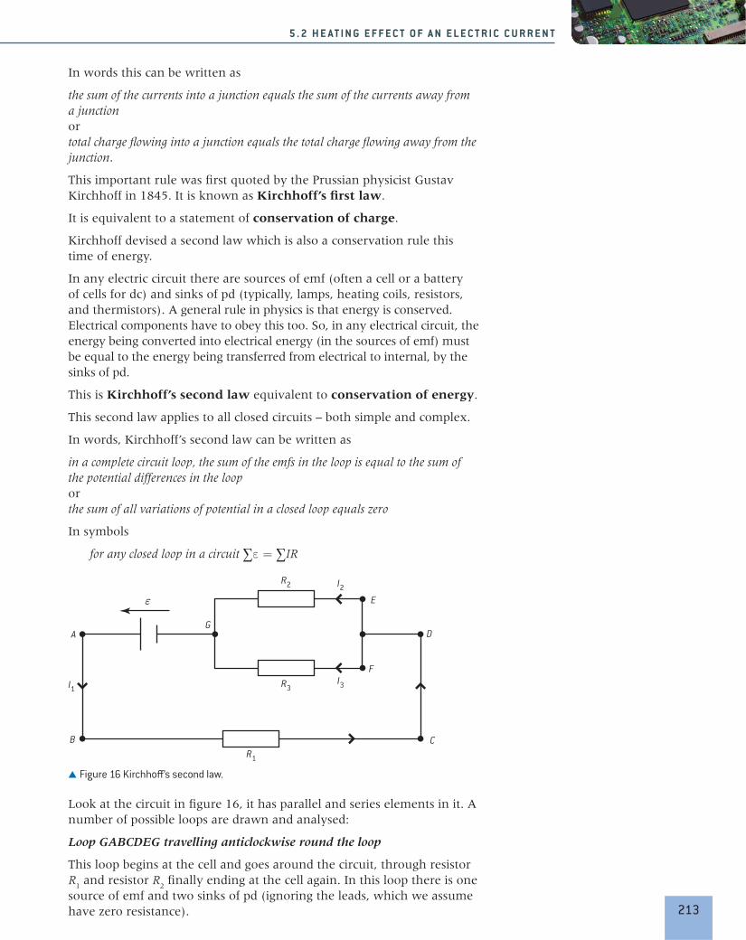
In words this can be written as

the sum of the currents into a junction equals the sum of the currents away from a junction or total charge flowing into a junction equals the total charge flowing away from the junction.

This important rule was first quoted by the Prussian physicist Gustav Kirchhoff in 1845. It is known as Kirchhoff’s first law.

It is equivalent to a statement of conservation of charge.

Kirchhoff devised a second law which is also a conservation rule this time of energy.

In any electric circuit there are sources of emf (often a cell or a battery of cells for dc) and sinks of pd (typically, lamps, heating coils, resistors, and thermistors). A general rule in physics is that energy is conserved. Electrical components have to obey this too. So, in any electrical circuit, the energy being converted into electrical energy (in the sources of emf) must be equal to the energy being transferred from electrical to internal, by the sinks of pd.

This is Kirchhoff’s second law equivalent to conservation of energy.

This second law applies to all closed circuits – both simple and complex.

In words, Kirchhoff’s second law can be written as

in a complete circuit loop, the sum of the emfs in the loop is equal to the sum of the potential differences in the loop or the sum of all variations of potential in a closed loop equals zero

In symbols

for any closed loop in a circuit ∑ε = ∑IR

R1

R3

R2 I2

E

D

I3

C

A

I1

B

F

G

ε

Figure 16 Kirchhoff’s second law.

Look at the circuit in figure 16, it has parallel and series elements in it. A number of possible loops are drawn and analysed:

Loop GABCDEG travelling anticlockwise round the loop

This loop begins at the cell and goes around the circuit, through resistor R1 and resistor R2 finally ending at the cell again. In this loop there is one source of emf and two sinks of pd (ignoring the leads, which we assume have zero resistance). 213


So

ε (the emf of the cell) = I1R1 + I2R2 (the total pds aross the resistors)

The direction of loop travel and the current direction are in all cases the same. We give a positive sign to the currents when this is the case. The emf of the cell is driving in the same direction as the loop travel direction; it gets a positive sign as well. If the loop direction and the current or emf were to be opposed then they would be given a negative sign.

loop EFGE travelling clockwise round the loop

This loop goes first through resistor R3 and the loop direction is in the same direction as the conventional current. Next the loop goes through resistor R1 but this time the current direction and the loop are different so there has to be a negative sign. There is no source of emf in the loop so the Kirchhoff equation becomes

0 = I3R3 – I2R2

Kirchhoff’s first law can be applied at point G. The total current into point G is I2 + I3; the total out is I1. The application of the law is I1 = I2 + I3.

There are now three separate equations with three unknowns and these equations can be solved to work out the currents in each part of the circuit assuming that we know the value for the emf of the cell and the values of the resistances in the circuit.

By setting up a series of loops it is possible to work out the currents and pds for complicated resistor networks, more complicated than could be done using the resistor series and parallel rules alone.

Ideal and non-ideal metersSo far in this topic we have assumed (without mentioning it!) that the meters used in the circuits were ideal. Ideal meters have no effect on the circuits that they are measuring. We would always want this to be true but, unfortunately, the meters we use in real circuits in the laboratory are not so obliging and we need to know how to allow for this.

Ammeters are placed in series with components so the ammeter has the same current as the components. It is undesirable for the ammeter to change the current in a circuit but, if the ammeter has a resistance of its own, then this is what will happen. An ideal ammeter has zero resistance – clearly not attainable in practice as the coils or circuits inside the ammeter have resistance.

Voltmeters are placed in parallel with the device or parts of a circuit they are measuring. In an ideal world, the voltmeter will not require any energy for its coil to move (if it is a moving-coil type) or for its analogue to digital conversion (if it is a digital meter). The way to avoid current in the voltmeter is for the meter to have an infinite resistance – again, not an attainable situation in practice.

Some modern digital meters can get very close to these ideals of zero ohm for ammeters and infinite ohms for voltmeters. Digital meters are used more and more in modern science.

214


Worked examples1 Calculate the unknown branch current in the

following junctions.

a)

9A 5A

3AI

b)

11A

5A

7A3A

I

Solutiona) Current into the junction = 9 + 5A

Current out of the junction = 3 + IA

I = 9 + 5 – 3 = 11 A out of the junction.

b) Current into the junction = I + 11 + 3 = I + 14A

Current out of the junction = 5 + 7 = 12A

I = 12 – 14 = –2 A, so the current I is directed away from the junction.

2 Calculate the currents in the circuit shown.

3.0 V

3.0 E

9.0 E

6.0 E

I1 I2

I3

Solution(This circuit can be analysed using the resistors in series and parallel equations. It is given here

to show the technique and to convince you that it works.)

3.0 V

3.0 E

junction A

loop 1

9.0 Eloop 2

6.0 E

I1 I2

I3

Current directions have been assigned and two loops 1 and 2 and junction A defined in the diagram.

For loop 1

3 = 3I1 + 9I2 [equation 1]

(the emf in the loop is 3 V)

for loop 2

0 = 6I3 – 9I2 [equation 2]

(there is no source of emf in this loop, current I2 is in the opposite direction to the loop direction 0.

For junction A

I1 = I2 + I3

so

0 = 9I2 – 6I1 + 6I2

0 = 15I2 – 6I1

And from equation 1

6 = 6I1 + 18I2

Adding the equations

6 = 33I2

I2 = 0.18 A

Substituting gives:

I1 = 0.45 A

and

I3 = 0.27 A

215


Nature of scienceHow times change!Digital meters are a good way to get very close to the ideal meter. The resistance between the input terminals can be made to be very large (1012 Ω or more) for a voltmeter and to have a very small value for an ammeter. The meters themselves are

easy to read without any judgements required about what the pointer indicates. It was not always like this.

An early form of meter was the hot-wire ammeter. This uses the heating effect of a current directly to increase the temperature of a metal wire (the current flows through the wire). There are a number of forms of the ammeter, but in the type shown here, a spring keeps the wire under tension. As the wire expands with the increase in temperature, any point on the wire moves to the right. A pivoted pointer is attached to the insulated thread. As the wire expands, the spring pulls the thread causing the pointer to rotate about the pivot; a reading of current can now be made. The scale is usually extremely non-linear.

spring

0

pivot

scale

resistance wire

meter terminals

path

thread

Figure 17

Worked examples1 A 250 Ω resistor is connected in series with a

500 Ω resistor and a 6.0 V battery.

a) Calculate the pd across the 250 Ω resistor.

b) Calculate the pd that will be measured across the 250 Ω resistor if a voltmeter of resistance 1000 Ω is connected in parallel with it.

Solutiona) The pd across the 250 Ω resistor

= Vin × R1 _ (R1 + R2)

6 × 250 _ (250 + 500)

= 2.0 V.

b) When the voltmeter is connected, the resistance of the parallel combination is

R = R1R2 _

(R1 + R2) = 250 × 1000 __

1250 = 200 Ω

V = 200 × 6 _ 700

= 1.7 V

2 An ammeter with a resistance of 5.0 Ω is connected in series with a 3.0 V cell and a lamp rated at 300 mA, 3 V. Calculate the current that the ammeter will measure.

SolutionResistance of lamp = V __ I = 3

___ 0.3 = 10 Ω . Total resistance in circuit = 10 + 5 = 15 Ω. So current in circuit = V __ R = 3 __ 15 = 200 mA. This assumes that the resistance of the lamp does not vary between 0.2 A and 0.3 A

216


Nature of scienceScientists need to balance their research into more and more efficient electric cells with the long-term risks associated with the disposal of the cells. Some modern cells have extremely poisonous contents. There will be serious consequences if these

chemicals are allowed to enter the water supply or the food chain. Can we afford the risk of using these toxic substances, and what steps should the scientists take when carrying forward the research?

Understanding Cells Primary and secondary cells Terminal potential difference Electromotive force emf Internal resistance

5.3 Electric cells

Applications and skills Investigating practical electric cells (primary

and secondary) Describing the discharge characteristic of a

simple cell (variation of terminal potential difference with time)

Identifying the direction current flow required to recharge a cell

Determining internal resistance experimentally Solving problems involving emf, internal

resistance, and other electrical quantities

Equation emf of a cell: ε = I(R + r)

IntroductionElectric currents can produce a chemical effect. This has great importance in chemical industries as it can be a method for extracting ores or purifying materials. However, in this course we do not investigate this aspect of the chemical effect. Our emphasis is on the use of an electric cell to store energy in a chemical form and then release it as electrical energy to perform work elsewhere.

CellsCells operate as direct-current (dc) devices meaning that the cell drives charge in one direction. The electron charge carriers leave the negative terminal of the cell. After passing around the circuit, the electrons re-enter the cell at the positive terminal. The positive terminal has a higher

217

5 . 3 E L E C T R I C C E L L S

potential than the negative terminal – so electrons appear to gain energy (whereas positive charge carriers would appear to lose it).

The chemicals in the cell are reacting while current flows and as a result of this reaction the electrons gain energy and continue their journey around the circuit.

Nature of scienceAnodes and cathodesYou will meet a naming system for anode and cathode which seems different for other cases in physics. In fact it is consistent, but you need to think carefully about it. For example, in a cathode-ray tube where the electrons in the tube are emitted from a hot metal filament, the filament is called the cathode and is at a negative voltage. This appears to be the opposite notation from that used for the electric cell. The reason is that the notation refers to what is happening inside the cell, not to the external circuit. The chemical reaction in the cell leads to positive

ions being generated at one of the electrodes and then flowing away into the bulk of the liquid. So as far as the interior of the cell is concerned this is an anode, because it is an (internal) source of positive ions. Of course, as far as the external circuit is concerned, the movement of positive charges away from this anode leaves it negative and the electrode will repel electrons in the external circuit. As external observers, we call this the negative terminal even though (as far as the interior of the cell is concerned) it is an anode.

Primary and secondary cellsMany of the portable devices we use today: torches, music players, computers, can operate with internal cells, either singly or in batteries. In some cases, the cells are used until they are exhausted and then thrown away. These are called primary cells. The original chemicals have completely reacted and been used up, and they cannot be recharged. Examples include AA cells (properly called dry cells) and button mercury cells as used in clocks and other small low-current devices.

On the other hand, some devices use rechargeable cells so that when the chemical reactions have finished, the cells can be connected to a charger. Then the chemical reaction is reversed and the original chemicals form again. When as much of the re-conversion as is possible has been achieved, the cell is again available as a chemical energy store. Rechargeable cells are known as secondary cells.

There many varieties of cell, here are two examples of the chemistry of a primary cell and that of a secondary cell.

The Leclanché cell was invented by Georges Leclanché in 1886. It is a primary cell and is the basis of many domestic torch and radio batteries.

218


- +carbon rodzinc rod

porous pot (P)

ammonium chloridesolution

glass vessel

Leclanché cell lead-acid accumulator

mixture of carbonand manganesedioxide

-+

negativeterminal

positive terminal

sulfuricacid

insulatingcase

leadlead oxide

gas vents

(a) (b)

Figure 1 Leclanché cell and lead-acid accumulator.

Figure 1(a) shows one practical arrangement of the cell. It consists of a zinc rod that forms the negative terminal. Inside the zinc is a paste of ammonium chloride separated from manganese dioxide (the cathode) by a porous membrane. In the centre of the manganese dioxide is a carbon rod that acts as the positive terminal for the cell.

Zinc atoms on the inside surface of the case oxidize to become positive ions. They then begin to move away from the inside of the case through the chloride paste leaving the case negatively charged. When the cell is connected to an external circuit, these electrons move around the circuit eventually reaching the carbon rod. A reaction inside the cell uses these electrons together with the components of the cell eventually forming the “waste products” of the cell, which include ammonia, manganese oxide, and manganese hydroxide.

Secondary cells are very important today. They include the lead–acid accumulator, together with more modern developments such as the nickel–cadmium (NiCd), nickel–metal-hydride (NiMH), and lithium ion cells. All these types can be recharged many times and even though they may have a high initial cost (compared to primary cells of an equivalent emf and capacity), the recharge is cheap so that, during the projected lifetime of the cell, the overall cost is lower than that of primary cells.

Although the lead-acid accumulator is one of the earliest examples of a secondary cell, it remains important (“accumulator” is an old word that implies the accumulation or collection of energy into a store). It is capable of delivering the high currents needed to start internal combustion and diesel engines, and it is reliable in the long term to maintain the current to important computer servers if the mains supply fails.

The lead–acid cell (figure 1(b)) is slightly older than the Leclanché cell, and was invented in 1859 by Gaston Planté.

In its charged state the cell consists of two plates, one of metallic lead, the other of lead(IV) oxide (PbO2) immersed in a bath of dilute sulfuric

219


acid. During discharge when the cell is supplying current to an external circuit, the lead plate reacts with the acid to form lead(II) sulfate and the production of two free electrons. The liquid surrounding the plates loses acid and becomes more dilute. At the oxide plate, electrons are gained (from the external circuit) and lead(II) sulfate is formed, also with the removal of acid from the liquid. So the net result of discharging is that the plates convert to identical lead sulfates and the liquid surrounding the plates becomes more dilute.

Recharging reverses these changes: electrons are forced from the positive plate by an external charging circuit and forced onto the negative plate. At the negative plate, atomic lead forms, at the positive, lead oxide is created, which restores the cell to its original state. The charge–recharge cycle can be carried out many times providing that the cell is treated carefully. However, if lead or lead oxide fall off the plates, they can no longer be used in the process and will collect at the bottom of the cell container. In the worst case the lead will short out the plates and the cell will stop operating. If the cell is overcharged (when no more sulfate can be converted into lead and lead oxide) the charging current will begin to split the water in the cell into hydrogen and oxygen gas which are given off from the cell. The total amount of liquid in the cell will decrease, meaning that the plates may not be fully covered by the acid. These parts of the plates will then not take part in the reaction and the ability of the cell to store energy will decrease.

Much industrial research effort is concentrated on the development of rechargeable cells. An important consideration for many manufacturers of electronic devices is the energy density for the battery (the energy stored per unit volume) as this often determines the overall design and mass of an electronic device. Also a larger energy density may well provide a longer lifetime for the device.

Capacity of a cellTwo cells with the same chemistry will generate the same electromotive force (emf) as each other. However if one of the cells has larger plates than the other and contains larger volumes of chemicals, then it will be able to supply energy for longer when both cells carry the same current.

The capacity of a cell is the quantity used to measure the ability of a cell to release charge. If a cell is discharged at a high rate then it will not be long before the cell is exhausted or needs recharging, if the discharge current is low then the cell will supply energy for longer times. The capacity of a cell or battery is the constant current that it can supply for a given discharge. So, if a cell can supply a constant current of 2 A for 20 hours then it said to have a capacity of 40 amp-hours (abbreviated as 40 A h).

The implication is that this cell could supply 1 A for 40 hours, or 0.1 A for 400 hours, or 10 A for 4 hours. However, practical cells do not necessarily discharge in such a linear way and this cell may be able to provide a small discharge current of a few milliamps for much

Worked examples1 Explain the difference

between a primary and a secondary cell.

Solution A primary cell is one that can convert chemical energy to electrical energy until the chemicals in the cell are exhausted. Recharging the cell is not possible.

A secondary cell can be recharged and the chemicals in it are converted back to their original form so that electrical energy can be supplied by the cell again.

2 A cell has a capacity of 1400 mA h. Calculate the number of hours for which it can supply a current of 1.8 mA.

SolutionCell capacity = current × time and therefore 1400 = 1.8t. In this case t = 780 hours.

220


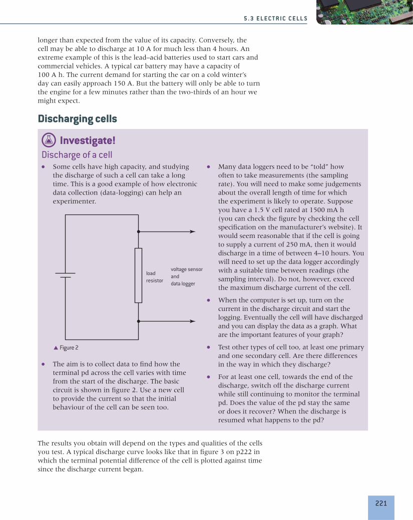
longer than expected from the value of its capacity. Conversely, the cell may be able to discharge at 10 A for much less than 4 hours. An extreme example of this is the lead–acid batteries used to start cars and commercial vehicles. A typical car battery may have a capacity of 100 A h. The current demand for starting the car on a cold winter’s day can easily approach 150 A. But the battery will only be able to turn the engine for a few minutes rather than the two-thirds of an hour we might expect.

Investigate!Discharge of a cell

Some cells have high capacity, and studying the discharge of such a cell can take a long time. This is a good example of how electronic data collection (data-logging) can help an experimenter.

loadresistor

voltage sensoranddata logger

Figure 2

The aim is to collect data to find how the terminal pd across the cell varies with time from the start of the discharge. The basic circuit is shown in figure 2. Use a new cell to provide the current so that the initial behaviour of the cell can be seen too.

Many data loggers need to be “told” how often to take measurements (the sampling rate). You will need to make some judgements about the overall length of time for which the experiment is likely to operate. Suppose you have a 1.5 V cell rated at 1500 mA h (you can check the figure by checking the cell specification on the manufacturer’s website). It would seem reasonable that if the cell is going to supply a current of 250 mA, then it would discharge in a time of between 4–10 hours. You will need to set up the data logger accordingly with a suitable time between readings (the sampling interval). Do not, however, exceed the maximum discharge current of the cell.

When the computer is set up, turn on the current in the discharge circuit and start the logging. Eventually the cell will have discharged and you can display the data as a graph. What are the important features of your graph?

Test other types of cell too, at least one primary and one secondary cell. Are there differences in the way in which they discharge?

For at least one cell, towards the end of the discharge, switch off the discharge current while still continuing to monitor the terminal pd. Does the value of the pd stay the same or does it recover? When the discharge is resumed what happens to the pd?

Discharging cells

The results you obtain will depend on the types and qualities of the cells you test. A typical discharge curve looks like that in figure 3 on p222 in which the terminal potential difference of the cell is plotted against time since the discharge current began.

221


0 20 40 60 80 100 120 140

0.9

1.0

1.1

1.2

1.3

time (minutes)ce

ll em

f / V

end of discharge(127 minutes)

midpoint voltage(1.18 volts)

Figure 3 Typical discharge–time graph for a cell.

Important features of this graph are that:

The initial terminal pd is higher than the quoted emf (the value the manufacturer prints on the case), but the initial value quickly drops to the rated emf (approximately).

For most of the discharge time the terminal pd remains more or less constant at or around the quoted emf. There is however sometimes a slow decline in the value of the terminal pd.

As the cell approaches exhaustion, the terminal pd drops very rapidly to a low level.

If the current is switched off, the terminal pd rises and can eventually reach the rated value again. However, when discharge is resumed, the terminal pd falls very quickly to the low value that it had before.

Other experiments are possible, particularly for rechargeable cells to see the effects of repeated discharge–charge cycles on the cell. Figure 4 shows how the capacity of a Ni–Cd cell changes as cell is taken through more and more cycles.

0 2500200015001000500

1

0

2

3

4

5

cycle number

cycle life at room temperature

capa

city

A h

Figure 4 Cycle life of a rechargeable cell.

222


Recharging secondary cellsThe clue to recharging a secondary cell is in the earlier descriptions of cell chemistry. The chemicals produce an excess of electrons at the negative terminal. During discharge these electrons then move through the external circuit transferring their energy as they go. When the electron arrives at the positive terminal, all of its energy will have been transferred to other forms and it will need to gain more from the chemical store in the cell.

To reverse the chemical processes we need to return energy to the cell using electrons as the agents, so that the chemical action can be reversed. When charging, the electrons need to travel in the reverse direction to that of the discharge current and you can imagine that the charger has to force the electrons the “wrong” way through the cell.

Part of a possible circuit to charge a 6-cell lead–acid battery is shown in figure 5.

-

+12–14 V dc

discharged battery

0–20 A

direction ofcharge flow

+14 V

0 V

A

Figure 5 Charging circuit for a cell.

The direction of the charging current is shown in the diagram. It is in the opposite direction to that of the cell when it is supplying energy. An input pd of 14 V is needed, notice the polarity of this input. The light-emitting diode (LED) and its series resistor indicate that the circuit is switched on. The ammeter shows the progress of charging. When the battery is completely discharged, the charging current will be high, but as the charging level (and therefore the emf) of the battery rises, this current gradually falls. During the charging process the terminal voltage will be greater than the emf of the cell. At full charge the emf of the battery is 13.8 V. When the current in the meter is zero, the battery is fully charged.

Internal resistance and emf of a cellThe materials from which the cells are made have electrical resistance in just the same way as the metals in the external circuit. This internal resistance has an important effect on the total resistance and current in the circuit.

223


(a)

rε

(b)

rE

R

A B

Figure 6

Figure 6(a) shows a simple model for a cell. Inside the dotted box is an “ideal” cell that has no resistance of its own. Also inside the box is a resistance symbol that represents the internal resistance of the cell. The two together make up our model for a real cell. The model assumes that the internal resistance is constant (for a practical cell it varies with the state of discharge) and that the emf is constant (which also varies with discharge current).

The model cell has an emf ε and an internal resistance r in series with an external resistance R (figure 6(b)). The current in the circuit is I.

We can apply Kirchhoff’s second law to this circuit:

the emf of the cell supplying energy to the circuit = εthe sum of the pds = IR + Ir

So

ε = IR + Ir

If the pd across the external resistor is V, then

ε = V + Ir

or

V = ε – Ir

It is important to realize that V, which is the pd across the external resistance, is equal to the terminal pd across the ideal cell and its internal resistance (in other words between A and B). The emf is the open circuit pd across the terminals of a power source – in other words, the terminal pd when no current is supplied. The pd between A and B is less than the emf unless the current in the circuit is zero. The difference between the emf and the terminal pd (the measured pd across the terminal of the cell) is sometimes referred to as the “lost pd” or the “lost volts”. These lost volts represent the energy required to drive the electron charge carriers through the cell itself. Once the energy has been used in the cell in this way, it cannot be available for conversion in the external circuit. You may have noticed that when a secondary cell is being charged, or any cell is discharging at a high current, the cell becomes warm. The energy required to raise the temperature of the cell has been converted in the internal resistance.

TOK

Simple assumptions

The model of a cell with a fixed internal resistance and a constant emf is an example of modelling. In this case the model is a simple one that cannot be realized in practice. Another model we used earlier was to suggest that there are ideal ammeters with zero resistance and ideal voltmeters with infinite resistance.

Scientists frequently begin with a very simple model of a system and then explore the possibilities that this model can offer in terms of analysis and behaviour. The next step is to make the model more complicated (but without being too intricate!) and to see how much complexity is needed before the model resembles the real system that is being modelled.

Do the simplifications and assumptions of ideal behaviour form a suitable basis for modelling?

224


Investigate!Measuring the internal resistance of a fruit cellThe method given here works for any type of electric cell, but here we use a citrus fruit cell (orange, lemon, lime, etc.) or even a potato for the measurement. The ions in the flesh of the fruit or the potato react with two different metals to produce an emf. With an external circuit that only requires a small current, the fruit cell can discharge over surprisingly long times.

Cu Zn

V

A

lemon

Figure 7

To make the cell, take a strip of copper foil and a strip of zinc foil, both about 1 cm by 5 cm and insert these, about 5 cm apart deep into the fruit. You may need to use a knife to make an incision unless the foil is stiff enough.

Connect up the circuit shown in figure 7 using a suitable variable resistor.

Measure the terminal pd across the fruit cell and the current in it for the largest range of pd you can manage.

Compare the equation

V = ε – Ir

with the equation for a straight line

y = c + mx

A plot of V on the y-axis against I on the x-axis should give a straight line with a gradient of –r and an intercept on the V-axis of ε.

A set of results for a cell (not a fruit cell in this case) is shown together with the corresponding graph of V against I. The intercept for this graph is 1.25 V and the gradient is –2.4 V A–1 giving an internal resistance value of 2.4 Ω.

0

0.2

0.4

0.6

0.8

1

1.2

1.4

term

inal

pd/

V

0 0.1 0.30.2 0.4 0.60.5current/A

Terminal pd / V Current / A

1.13 0.05

1.01 0.10

0.89 0.15

0.77 0.20

0.65 0.25

0.53 0.30

0.41 0.35

0.29 0.40

0.17 0.45

0.05 0.50

Figure 8

225


Worked example1 A cell of emf 6.0 V and internal resistance 2.5 Ω

is connected to a 7.5 Ω resistor.

Calculate:

a) the current in the cell

b) the terminal pd across the cell

c) the energy lost in the cell when charge flows for 10 s.

Solution a) Total resistance in the circuit is 10 Ω, so

current in circuit = 6 __ 10 = 0.60 A

b) The terminal pd is the pd across cell = IR =

0.6 × 7.5 = 4.5 V

c) In 10 s, 6 C flows through the cell and the energy lost in the cell is 1.5 J C–1. The energy lost is 9.0 J.

2 A battery is connected in series with an ammeter and a variable resistor R. When R = 6.0 Ω, the current in the ammeter is 1.0 A. When R = 3.0 Ω, the current is 1.5 A. Calculate the emf and the internal resistance of the battery.

Solution Using

V = ε – Ir

and knowing that V = IR gives two equations:

6 × 1 = ε – 1 × r

and

3 × 1.5 = ε – 1.5 × r

These can be solved simultaneously to give (6 – 4.5) = 0.5r or r = 3.0 Ω and ε = 9.0 V.

Power supplied by a cellThe total power supplied by a non-ideal cell is equal to the power delivered to the external circuit plus the power wasted in the cell. Algebraically,

P = I2 R + I2 r

using the notation used earlier.

The power delivered to the external resistance is

ε2 _

(R + r)2 R

00

load resistance Rr

powe

r del

iver

edto

load

resi

stor

Figure 9 Power delivered to a resistor.

Figure 9 shows how the power that is delivered to the external circuit varies with R. The peak of this curve is when r = R, in other words, when the internal resistance of the power supply is equal to the resistance of the external circuit. The load and the supply are “matched” when the resistances are equal in this way. This matching of supply and circuit is important in a number of areas of electronics.

Worked exampleA battery of emf 9.0 V and internal resistance 3.0 Ω is connected to a load resistor of resistance 6.0 Ω. Calculate the power delivered to the external load.

Solution Using the equation ε2

______ (R + r)2 R

leads to 92

_____ (6+3)2 6 = 6.0 W

226


5.4 Magnetic effects of electric currents

Nature of scienceSometimes visualization aids our understanding. Magnetic field lines are one of the best examples of this. Scientists began by visualizing the shape and strength of a magnetic field through the

position and direction of the fictitious lines of force (or field lines). The image proved to be so powerful that the technique was subsequently used with electric and gravitational fields too.

Understanding Magnetic fields Magnetic force

Applications and skills Sketching and interpreting magnetic field patterns Determining the direction of the magnetic field

based on current direction Determining the direction of force on a charge

moving in a magnetic field Determining the direction of force on a current-

carrying conductor in a magnetic field Solving problems involving magnetic forces,

fields, current and charges

Equations force on a charge moving in a magnetic field:

F = qvB sin θ force on a current-carrying conductor in a

magnetic field: F = ILB sin θ

IntroductionElectromagnetism is the third effect observed when charge moves in a circuit – the electric current gives rise to a magnetic field. But it was not the observation of a magnetic effect arising from a current in a wire that began the ancient study of magnetism. Early navigators knew that some rocks are magnetic. As with the nature of electric charge, the true origins of magnetic effects remained obscure for many centuries. Only comparatively recently has an understanding of the microscopic aspects of materials allowed a full understanding of the origins of magnetism. As with electrostatics, scientists began by using the concept of the field to describe the behaviour of interacting magnets. However, magnetic fields differ fundamentally in character from electrostatic fields and are in some ways more complex.

Magnetic field patternsThe repulsion between the like poles of two bar magnets is familiar to us. The forces between magnets of even quite modest strength are impressive. Modern magnetic alloys can be used to produce tiny magnets

227

5 . 4 M A G N E T I C E F F E C T S O F E L E C T R I C C U R R E N T S

Nature of scienceTalking about polesA word about notation: there is a real possibility of confusion when talking about magnetic poles. This partly arises from the origin of our observations of magnetism. When we write “magnetic north pole” what we really mean is “the magnetic pole that seeks the geographic north pole” (figure 1(a)). We often talk loosely about a magnetic north pole pointing to the north pole. Misunderstandings can occur here because we also know that like poles repel and unlike poles attract. So we end up with the situation that a magnetic north pole is attracted to the “geographic north pole” – which seems wrong in the context of two poles repelling. In this book we will talk about north-seeking poles meaning “geographic north-seeking” and south-seeking poles meaning “geographic south seeking”. On the diagrams, N will mean geographic north seeking, S will mean geographic south seeking.

Figure 1(b) shows the patterns for a single bar magnet and (c) and (d) two arrangements of a pair of bar magnets of equal strength.

S

N

(a)

N S

(b)

(d)

(c)

S N

N N

Figure 1 Magnetic field patterns.

(less than 1 cm in diameter and a few millimetres thick) that can easily attract another ferromagnetic material through significant thicknesses of a non-magnetic substance.

At the beginning of a study of magnetism, it is usual to describe the forces in terms of fields and field lines. You may have met this concept before. There is said to be a magnetic field at a point if a force acts on a magnetic pole (in practice, a pair of poles) at that point. Magnetic fields are visualized through the construction of field lines.

Magnetic field lines have very similar (but not identical) properties to those of the electric field lines in Sub-topic 5.1. In summary these are:

Magnetic field lines are conventionally drawn from the north-seeking pole to the south-seeking pole, they represent the direction in which a north-seeking pole at that point would move.

The strength of the field is shown by the density of the field lines, closer lines mean a stronger field.

The field lines never cross.

The field lines act as though made from an elastic thread, they tend to be as short as possible.

228


In the pairs, notice the characteristic field pattern when the two opposite poles are close (figure 1(b)) and when the two north-seeking poles are close (figure 1(c)). When two north-seeking poles are close (or two south-seeking poles), there is a position where the field

is zero between the magnets (called a null point). When two opposite poles are close, the field lines connect the two magnets. In this situation the magnets will be attracted, so this particular field pattern implies an attraction between poles.

Investigate!Observing field patterns of permanent magnets and electric currents

There are a number of ways to carry out this experiment. They can involve the scattering of small iron filings, observation of suspensions of magnetized particles in a special liquid, or other techniques. This Investigate! is based on the iron-filing experiment but the details will be similar if you have access to other methods.

Take a bar magnet and place a piece of rigid white card on top of it. You may need to support the card along its sides. Choose a non-magnetic material for the support.

Take some iron filings in a shaker (a pepper pot is ideal) and, from a height above the card of about 20 cm sprinkle filings onto the card. It is helpful to tap the card gently as the filings fall onto it.

You should see the field pattern forming as the magnetic filings fall through the air and come under the influence of the magnetic field. Sketch or photograph the arrangement.

The iron filings give no indication of field direction. The way to observe this is to use a plotting compass – a small magnetic compass a few centimetres in diameter – that indicates the direction to which a north-seeking pole sets itself. Place one or more of these compasses on the card and note the direction in which the north-seeking pole points.

Repeat with two magnets in a number of configurations; try at least the two in figure 1.

Electric currents also give rise to a magnetic field. However, currents small enough to be safe will only give weak fields, not strong enough to affect the filings as they fall.

To improve the effect: cut a small hole in the centre of the card and run a long lead through it (the lead will need to be a few metres long). Loop the lead in the same direction through a number of times (about ten turns if possible). This trick enables one current to contribute many times to the same field pattern. You may need at least 25 A in total (2.5 A in the lead) to see an effect.

Figure 2

229


Magnetic field due to a current in conductorsThe magnetic field pattern due to a current in a long straight wire is a circular pattern centred on the wire. This seems odd to anyone only used to the bar magnet pattern. Measurements show that the field is strong close to the wire but becomes weaker further away from it. This should be clear in your drawings of the long wire field pattern when the lines of force are drawn at increased spacing as you move further from the wire.

point of arrow indicates current leaving page towards you

tail of arrow indicates current entering page away from you

lines of magneticfield

south pole

north pole

Figure 3 Magnetic field patterns around current-carrying conductors.

Your observations using the plotting compasses should have shown that the direction of the field depends on the direction of the current.

Using the conventional current (i.e. the direction that positive charges are moving in the wire) the relationship between the current and the magnetic field direction obeys a right-hand corkscrew rule relationship.

To remember this, hold your right hand with the fingers curled into the palm and the thumb extended away from the fingers (see figure 4). The thumb represents the direction of the conventional current and the fingers represent the direction of the field. Another way to think of the current–field relationship is in terms of a

thumb points in directionof conventional current

current flow

fingers curl around the conductor(indicating the direction of magnetic field)

Figure 4 Right-hand corkscrew rule.

230


screwdriver being used to insert a screw. The screwdriver has to turn a right-handed screw clockwise to insert it and drive the screw forwards. The direction in which the imaginary screw moves is that of the conventional current, and the direction in which the screwdriver turns is that of the field.

Use whichever direction rule you prefer, but use it consistently and remember that the rule works for conventional current.

The strength of the magnetic field can be increased by increasing the current in the conductor.

The magnetic field due to the solenoid is familiar to you already. To understand how it arises, you need to imagine the long straight wire being coiled up into the solenoid shape taking its circular field with it as the coiling takes place. With current in the wire, the circular field is set up in each wire. This circular field adds together with fields from neighbouring turns in the solenoid. Figure 5 shows this; look closely at what happens close to the individual wires. The black lines show the field near the wires, the blue lines show how the fields begin to combine, the red line shows the combined field in the centre of the solenoid.

circularfield

near turn

consecutiveturns on solenoid

fields addtogether

Figure 5 Building up the field pattern.

A field runs along the hollow centre of the solenoid and then outside around the solenoid (figure 3). Outside it is identical to the bar magnet pattern to the extent that we can assign north- and south-seeking poles to the solenoid. Again there is an easy way to remember this using an N and S to show the north-seeking and south-seeking poles. The arrows on the N and S show the current direction when looking into the solenoid from outside. If you look into the solenoid and the conventional current is anticlockwise at the end of the solenoid closer to you then that is the end that is north-seeking. If the current is clockwise then that is the south-seeking end.

The strength of the magnetic field in a solenoid can be increased by:

increasing the current in the wire

increasing the number of turns per unit length of the solenoid

adding an iron core inside the solenoid.

anticlockwisecurrent gives a

north seeking pole

clockwisecurrent gives a

south seeking pole

Figure 6 Right hand corkscrew rule and pole direction.

231


Worked exampleFour long straight wires are placed perpendicular to the plane of the paper at the edges of a square.

The same current is in each wire in the direction shown in the diagram. Deduce the direction of the magnetic field at point P in the centre of the square.

P

SolutionThe four field directions are shown in the diagram. The sum of these four vectors is another vector directed from point P to the left.

BA

D C

P

D

CA

B

Nature of scienceBut why permanent magnets?We have said nothing about the puzzle of permanent magnets or the magnetism of the Earth (Figure 1(a)). The suggestion is that magnetism arises between charges when the charges move relative to each other. Can this idea be extended to help explain the reasons for permanent magnetism (known as ferromagnetism)? In fact, permanent magnetism is comparatively rare in the periodic table, only iron, nickel, and cobalt and alloys of these metals show it.

The reason is due to the arrangement of the electrons in the atoms of these substances. Electrons are now known to have the property of spin which can be imagined as an orbiting motion around the atom. In iron, cobalt and nickel, there is a particular arrangement that involves an unpaired electron. This is the atomic origin of the moving charge that is needed for a magnetic field to appear.

The second reason why iron, nickel, and cobalt are strong permanent magnets is that neighbouring atoms can co-operate and line up the spins of their unpaired electrons in the same direction. So, many electrons are all spinning in the same direction and giving rise to a strong magnetic field.

Deep in the centre of the Earth it is thought that a liquid-like metallic core containing free electrons is rotating relative to the rest of the planet. Again, these are conditions that can lead to a magnetic field. In which direction do you predict that the electrons are moving? However, this phenomenon is not well understood and is still the subject of research interest. Why, for example, does the magnetic field of the Earth flip every few thousand years? There is much evidence for this including the magnetic “striping” in the undersea rocks of the mid-Atlantic ridge and in the anomalous magnetism found in some ancient cooking hearths of the aboriginal peoples of Australia.

232


Forces on moving chargesForce between two current-carrying wiresWe have used field ideas to begin our study of magnetic effects, but these conceal from us the underlying physics of magnetism. To begin this study we look at the interactions that arise between conductors when they are carrying electric current.

(a)

foil strips

+ -

-

+

(b) (c)

current out of pagecurrent into pagecurrents in same directions

Figure 7

Figure 7(a) shows two foil strips hanging vertically. The current directions in the foils can be the same or opposite directions. When the currents are in the same direction, the strips move together due to the force on one foil strip as it sits in the magnetic field of the other strip. When the currents are in opposing directions, the strips are seen to move apart.

You can set this experiment up for yourself by using two pieces of aluminium foil about 3 cm wide and about 70 cm long for each conductor. The power supply should be capable of providing up to 25 A so take care! Connections are made to the foils using crocodile (alligator) clips.

233


The forces on the foil can be explained in terms of the interactions between the fields as shown in the figure 7(b). When the currents are in the same direction, the field lines from the foils combine to give a pattern in which field lines loop around both foils. The notation used to show the direction of conventional current in the foil is explained on the diagram. Look back at figure 1(d) which shows the field pattern for two bar magnets with the opposite poles close. You know that the bar magnets are attracted to each other in this situation. The field pattern for the foils is similar and also leads to attraction. Think of the field lines as trying to be as short as possible. They become shorter if the foils are able to move closer together.

When the currents are in opposite directions, the field pattern changes (figure 7(c)). Now the field lines between the foils are close together and in the same direction thus representing a strong field. It seems reasonable that a strong magnetic field (like a strong electrostatic field) represents a large amount of stored energy. This energy can be reduced if the foils move apart allowing the field lines to separate too. Again, this has similarities to the bar magnet case but this time with like poles close together.

Force between a bar magnet field and a current-carrying wireOne extremely important case is the interaction between a uniform magnetic field and that produced by a current in a wire.

Again we can start with the field between two bar magnets with unlike poles close. In the centre of the region between the magnets, the field is uniform because the field lines are parallel and equally spaced.

SN S + =

(a) (b)

force on wire

N

Figure 8 The catapult field.

Suppose a wire carrying a current sits in this field. Figure 8(a) shows the arrangement and the directions of the uniform magnetic field and the field due to the current. A force acts downwards on the wire.

The effect can again be explained in terms of the interaction between the two magnetic fields. The circular field due to the wire adds to the uniform field due to the magnets to produce a more complicated field. This is shown in figure 8(b). Overall, the field is weaker below the wire than above it. Using our ideas of the field lines, it is clear that the system (the wire and the uniform field) can overcome this difference in field strength, either by attempting to move the wire downwards or by moving the magnets that cause the uniform field upwards. This effect

234


is sometimes called the catapult field because the field lines above the wire resemble the stretched elastic cord of a catapult just before the object in the catapult is fired.

This effect is of great importance to us. It is the basis for the conversion of electrical energy into kinetic energy. It is used in electric motors, loudspeakers, and other devices where we need to produce movement from an electrical power source. It is called the motor effect.

It is possible to predict the direction of motion of the wire by drawing the field lines on each occasion when required but this is tedious. There are a number of direction rules that are used to remember the direction of the force easily. One of the best known of these is due to the English physicist Fleming and is known as Fleming’s left-hand rule.

field alongF irst finger

left handcurrent alongseCond finger

force (motion) along thuMb

B

I

F

Figure 9 Fleming’s left-hand rule.

To use the rule, extend your left hand as shown in figure 9. Your first (index) finger points in the direction of the uniform magnetic field and your second finger points in the direction of the conventional current in the wire, then your thumb gives the direction of the force acting on the wire.

The motor effectThe explanation for the motor effect has been given so far in terms of field lines. This is, of course, not the complete story. We should be looking for explanations that involve interactions between individual charges, both those that produce the uniform magnetic field and those that arise from the current in the wire. Electrostatic effects (as their name implies) arise between charges that are not moving. Magnetic effects arise because the sets of charges that produce the fields are moving relative to each other and are said to be in different frames of reference. There have been no electrostatic effects because we have dealt with conductors in which there is an exact balance of positive and negative charges. Magnetism can be thought of as the residual effect that arises when charges are moving with respect to each other.

235


Worked exampleWires P and R are equidistant from wire Q.

wire P

I

wire Q

I

wire R

I

Each wire carries a current of the same magnitude and the currents are in the directions shown.

Describe the direction of the force acting on wire Q due to wires P and R.

SolutionUsing the right-hand corkscrew rule, the field due to wire P at wire Q is out of the plane of the paper, and the field due to wire R at wire Q is also out of the plane of the paper.

Using Fleming’s left-hand rule, the force on wire Q is in the plane of the paper and to the left.

The magnitude of the magnetic force

Investigate!Force on a current-carrying conductor

C 0

magnets on steel yoke

balance

current carrying lead

l

Figure 10

This is an experiment that will give you an idea of the size of the magnetic force that acts on typical laboratory currents. If carried out carefully it will also allow you to see how the force varies with the length of the conductor and the size of the current.

You will need some pairs of flat magnets (known as “magnadur” magnets, a sensitive top-pan balance, a power supply and a suitable long straight lead to carry the current.

Arrange the apparatus as shown in the diagram.

Zero the balance so that the weight of the magnets is removed from the balance reading.

The experiment is in two parts:

First, vary the current in the wire and collect data for the force acting on the magnets, and therefore the balance, as a result. A trick to improve precision is to reverse the current in the wire and take balance readings for both directions. Then add the two together (ignoring the negative sign of one reading) to give double the answer. Draw a graph to display your data.

Second, use two pairs of magnets side-by-side to double the length of the field. Take care that the poles match, otherwise the forces will cancel out. This is not likely to work so well as you need to assume that the magnet pairs have the same strength. This will probably not be true. But, roughly speaking, does doubling the length of wire in the field double the force?

236


The result of experiments like the one above is that the force acting on the wire due to the field is proportional to:

the length (l) of the wire

the current (I) in the wire.

This leads us to a definition of magnetic field strength rather different from that of electric field strength and gravitational field strength.

We cannot define the magnetic field strength in terms of

force __ a single quantity

because the force depends on two quantities: current and length.

Instead we define

magnetic field strength

= force acting on a current element

_____ current in the element × length of the element

By “element” we mean a short section of a wire that carries a current. If a force F acts on the element of length l when the current in it is I, then the magnetic field strength B is defined by

B = F _ Il

B

(a) (b)F = BIl

lB

F = BIl sinθ

l

θ

Figure 11

The unit of magnetic field strength is the tesla, abbreviated T and the tesla is equivalent to the fundamental units kg s–2 A–1. When a 1 metre long current element is in a magnetic field and has a current of 1 A in it, if a magnetic force of 1 N acts on it, then the magnetic field strength is defined to be 1 T. The tesla can also be thought of as a shortened form of N A-1 m-1. The tesla turns out to be a very large unit indeed. The largest magnetic field strengths created in a laboratory are a few kT and the magnetic field of the Earth is roughly 10–4 T. The very largest fields are associated with some neutron stars. The field strength can be order of 100 GT in such stars.

Having defined B we can go on to rearrange the equation to give the force that acts on a wire:

F = BIl

This applies when the field lines, the current and the wire are all at 90° to each other as they are when you use the Fleming left-hand rule. If this is not the case (see figure 11(b)) and the wire is at an angle θ to the lines then we need to take the appropriate component of I or l that is at 90° to the field.

237


In terms of the way the angle is defined in figure 11(b), the equation becomes

F = BIl sin θThis equation is written in terms of the current in the wire. Of course, the current is, as usual, the result of moving charge carriers. The equation can be changed to reflect this.

From Sub-topic 5.1 we know that the current I is given by

I = Q

_ t

where Q is the charge that flows through the current element taking a time t to do it.

Substituting

F = B ( Q _ t ) l sin θ

= BQ ( l _ t ) sin θ

The term ( l _ t ) is the drift speed v of the charge carriers and making this

substitution gives the expression

F = BQv sin θfor the force acting on a charge Q moving at speed v at an angle θ to a magnetic field of strength B.

Notice the way that the angle θ is defined in the diagrams. It is the angle between the direction in which the charge is moving (or the current direction – the same thing) and the field lines. Don’t get this wrong and use cosine instead of sine in your calculations.

TOK

Why direction rules?

During this sub-topic we have introduced two direction rules: the corkscrew rule for magnetic fields around wires and Fleming’s rule for the motor effect. What is the status of these rules? Are they implicit in the way the universe operates, or are they simply indications that depend on the way we define current direction and other fundamental quantities in physics? To begin to answer this, consider what would have happened if Franklin had known that charge carriers in metals were electrons with a negative charge. What would this have changed (if anything)?

Nature of scienceThe definition of the ampereIn Topic 1 you learnt that the ampere was defined in terms of the force between two current-carrying wires. You may have thought this odd both then and when the relationship between current and charge was developed earlier in this topic. Perhaps it is clearer now.

A precise measurement of charge is quite difficult. At one time it could only be achieved through chemical measurements of electrolysis – and the levels of precision were not great enough to give a good value at that time.

It is much easier to set up an experiment that measures the force between two wires. The experiment can be done to a high precision using a device called a current balance (as in the force Investigate! above) in which the magnetic force can be measured in terms of the gravitational force needed to cancel it out. This is rather like old-fashioned kitchen scales where the quantity being measured is judged against a standard mass acted on by gravity.

238


Worked example1 When a charged particle of mass m, charge q

moves at speed v in a uniform magnetic field then a magnetic force F acts on it. Deduce the force acting on a particle mass m of charge 2q and speed 2v travelling in the same direction in the same magnetic field.

SolutionThe equation for the force is F = BQv sin θ In the equation, sin θ and B do not change but every other quantity does, so the force is 4F.

2 Electric currents of magnitude I and 3I are in wires 1 and 2 as shown.

wire 1

I 3I

wire 2

A force F acts on wire 2 due to the current in wire 1. Deduce the magnitude of the force on wire 1 due to the current in wire 2.

Solution This problem can be solved by reference to Newton’s laws of motion, but an alternative is to consider the changes in magnetic field. If the magnetic field at wire 2 due to wire 1 is B then the magnetic field at wire 1 due to wire 2 is 3B. However, the current in wire 1 is one-third of that in wire 2.

So force at wire 1 due to wire 2 is

F = 3B × I __ 3 × l = force in wire 2 due to wire 1.

The forces are the same.

Nature of scienceVectors and their productsYou may have formed the view that vectors are just used for scale diagrams in physics. This is not the case, vectors come into their own in mathematical descriptions of magnetic force.

There is only one way to multiply scalars together: run a relay with four stages each of distance 100 m and the total distance travelled by the athletes is 400 m. Multiplying two scalars only gives another scalar.

Vectors, because of the added direction, can be multiplied together in two ways:

to form a scalar product (sometimes called “dot” product) where, for example, force and displacement are multiplied together to give work done (a scalar) that has no direction. In vector notation this is written as F·s = W. The multiplication sign is the dot (hence the name) the vectors are written with a bold font, the scalar in ordinary font.

to form a vector product (sometimes called “cross” product) where two vectors are

multiplied together to give a third vector, thus a × b = c

The multiplication of qv and B to form the vector force F is a vector product. The charge q is a scalar but everything else in the equation is a vector. A mathematician would write

F = q (v × B)

to show that the vector velocity and the vector magnetic field strength are multiplied together. The order of v and B is important. There is a vector rule for the direction of F that is consistent with our observations earlier and the sin θ appears when the vector multiplication is worked out in terms of the separate components of the vector.

Vector notation turns out to be an essential language of physics, because it allows a concise notation and because it contains all the direction information within the equations rather than forcing us to use direction rules. However we do not pursue the full theory of vectors in IB Physics.

239


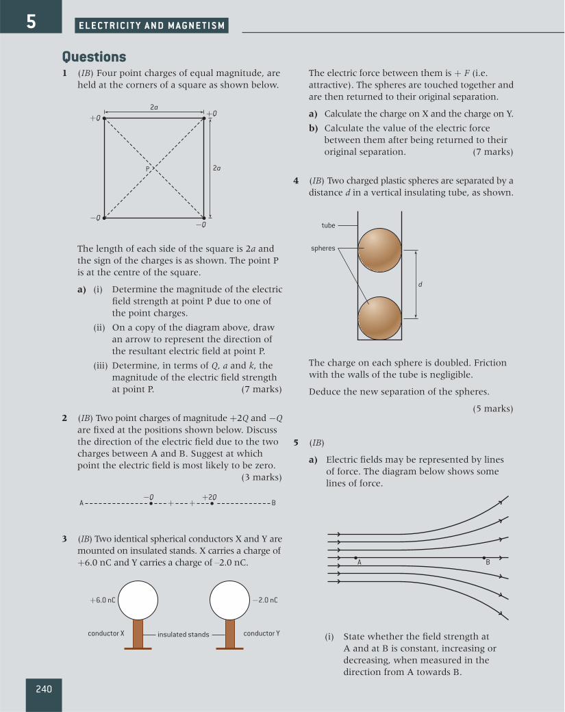
Questions1 (IB) Four point charges of equal magnitude, are

held at the corners of a square as shown below.

2a

2a

+Q

−Q

+Q

P

−Q

The length of each side of the square is 2a and the sign of the charges is as shown. The point P is at the centre of the square.

a) (i) Determine the magnitude of the electric field strength at point P due to one of the point charges.

(ii) On a copy of the diagram above, draw an arrow to represent the direction of the resultant electric field at point P.

(iii) Determine, in terms of Q, a and k, the magnitude of the electric field strength at point P. (7 marks)

2 (IB) Two point charges of magnitude +2Q and −Q are fixed at the positions shown below. Discuss the direction of the electric field due to the two charges between A and B. Suggest at which point the electric field is most likely to be zero. (3 marks)

A B+2Q−Q + +

3 (IB) Two identical spherical conductors X and Y are mounted on insulated stands. X carries a charge of +6.0 nC and Y carries a charge of –2.0 nC.

+6.0 nC −2.0 nC

conductor X conductor Yinsulated stands

The electric force between them is + F (i.e. attractive). The spheres are touched together and are then returned to their original separation.

a) Calculate the charge on X and the charge on Y.

b) Calculate the value of the electric force between them after being returned to their original separation. (7 marks)

4 (IB) Two charged plastic spheres are separated by a distance d in a vertical insulating tube, as shown.

tube

d

spheres

The charge on each sphere is doubled. Friction with the walls of the tube is negligible.

Deduce the new separation of the spheres.

(5 marks)

5 (IB)

a) Electric fields may be represented by lines of force. The diagram below shows some lines of force.

A B

(i) State whether the field strength at A and at B is constant, increasing or decreasing, when measured in the direction from A towards B.

E L E C T R I C I T Y A N D M A GN E T I S M5

240

(ii) Explain why field lines can never touch or cross.

b) The diagram below shows two insulated metal spheres. Each sphere has the same positive charge.

++

Copy the diagram and in the shaded area between the spheres, draw the electric field pattern due to the two spheres. (8 marks)

6 (IB) A lamp is at normal brightness when there is a potential difference of 12 V across its filament and a current in the filament of 0.50 A.

a) For the lamp at normal brightness, calculate:

(i) the power dissipated in the filament

(ii) the resistance of the filament.

b) In order to measure the voltage–current (V–I) characteristics of the lamp, a student sets up the following electrical circuit.

12 V battery

State the correct positions of an ideal ammeter and an ideal voltmeter for the characteristics of the lamp to be measured.

c) The voltmeter and the ammeter are connected correctly in the previous circuit. Explain why the potential difference across the lamp

(i) cannot be increased to 12 V

(ii) cannot be reduced to zero.

d) An alternative circuit for measuring the V–I characteristic uses a potential divider.

(i) Draw a circuit that uses a potential divider to enable the V–I characteristics of the filament to be found.

(ii) Explain why this circuit enables the potential difference across the lamp to be reduced to 0 V. (13 marks)

7 (IB) The graph below shows the V–I characteristic for two 12 V filament lamps A and B.

0

12

0.5

lamp Alamp B

0 1.0current/A

pote

ntia

l diff

eren

ce/V

a) (i) Explain why the graphs indicate that these lamps do not obey Ohm’s law.

(ii) State and explain which lamp has the greater power dissipation for a potential difference of 12 V.

The two lamps are now connected in series with a 12 V battery as shown below.

12 V battery

lamp A lamp B

b) (i) State how the current in lamp A compares with that in lamp B.

(ii) Use the V–I characteristics of the lamps to deduce the total current from the battery.

(iii) Compare the power dissipated by the two lamps. (11 marks)

241

Q U E S T I O N S

241

8 (IB)

a) Explain how the resistance of the filament in a filament lamp can be determined from the V–I characteristic of the lamp.

b) A filament lamp operates at maximum brightness when connected to a 6.0 V supply. At maximum brightness, the current in the filament is 120 mA.

(i) Calculate the resistance of the filament when it is operating at maximum brightness.

(ii) You have available a 24 V supply and a collection of resistors of a suitable power rating and with different values of resistance. Calculate the resistance of the resistor that is required to be connected in series with the supply such that the voltage across the filament lamp will be 6.0 V. (4 marks)

9 (IB) The graph below shows the I–V characteristics for component X.

4

2

20-2-4-6-8 4 6 80

-2

-4

-6

6I/A

V/V

The component X is now connected across the terminals of a battery of emf 6.0 V and negligible internal resistance.

a) Use the graph to determine:

(i) the current in component X

(ii) the resistance of component X.

b) A resistor R of constant resistance 2.0 Ω is now connected in series with component X as shown below.

2.0 Ω

R

E

X

(i) Copy the graph in (a), and draw the I–V characteristics for the resistor R.

(ii) Determine the total potential difference E that must be applied across component X and across resistor R such that the current through X and R is 3.0 A. (7 marks)

10 (IB) A student is to measure the current–voltage (I–V) characteristics of a filament lamp. The following equipment and information are available.

Information

Battery emf = 3.0 V, negligible internal resistance

Filament lamp marked “3 V, 0.2 A”

Voltmeter resistance = 30 kΩ, reads values between 0.0 and 3.0 V

Ammeter resistance = 0.1 Ω, reads values between 0.0 and 0.5 A

Potentiometer resistance = 100 Ωa) For the filament lamp operating at normal

brightness, calculate:

(i) its resistance

(ii) its power dissipation.

The student sets up the following incorrect circuit.

V

A

b) (i) Explain why the lamp will not light.

(ii) State the approximate reading on the voltmeter. Explain your answer. (6 marks)

242


242

5

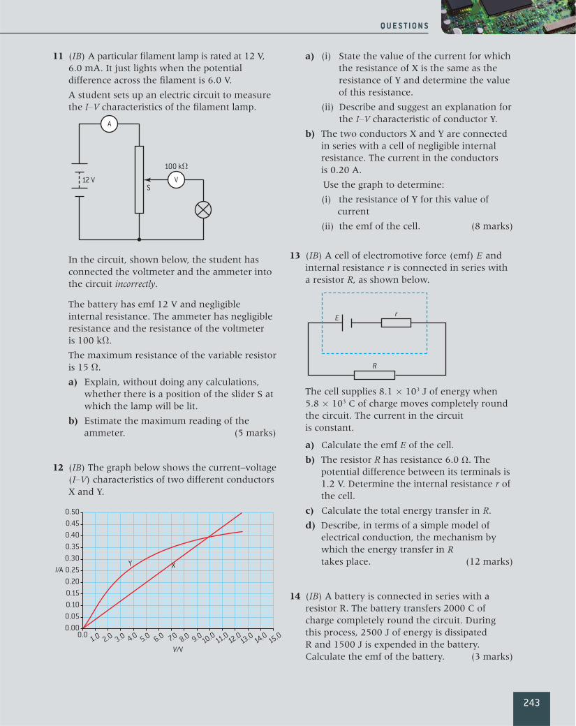
11 (IB) A particular filament lamp is rated at 12 V, 6.0 mA. It just lights when the potential difference across the filament is 6.0 V.

A student sets up an electric circuit to measure the I–V characteristics of the filament lamp.

A

V

100 kΩ12 V

S

In the circuit, shown below, the student has connected the voltmeter and the ammeter into the circuit incorrectly.

The battery has emf 12 V and negligible internal resistance. The ammeter has negligible resistance and the resistance of the voltmeter is 100 kΩ.

The maximum resistance of the variable resistor is 15 Ω.

a) Explain, without doing any calculations, whether there is a position of the slider S at which the lamp will be lit.

b) Estimate the maximum reading of the ammeter. (5 marks)

12 (IB) The graph below shows the current–voltage (I–V) characteristics of two different conductors X and Y.

0.00.000.050.100.150.200.250.300.350.400.450.50

Y X

1.0 2.0 3.0 4.0 5.0 6.0 7.0 8.0 9.0 10.0 11.0 12.013.0 14.0 15.0

V/V

I/A

a) (i) State the value of the current for which the resistance of X is the same as the resistance of Y and determine the value of this resistance.

(ii) Describe and suggest an explanation for the I–V characteristic of conductor Y.

b) The two conductors X and Y are connected in series with a cell of negligible internal resistance. The current in the conductors is 0.20 A.

Use the graph to determine:

(i) the resistance of Y for this value of current

(ii) the emf of the cell. (8 marks)

13 (IB) A cell of electromotive force (emf) E and internal resistance r is connected in series with a resistor R, as shown below.

r

R

E

The cell supplies 8.1 × 103 J of energy when 5.8 × 103 C of charge moves completely round the circuit. The current in the circuit is constant.

a) Calculate the emf E of the cell.

b) The resistor R has resistance 6.0 Ω. The potential difference between its terminals is 1.2 V. Determine the internal resistance r of the cell.

c) Calculate the total energy transfer in R.

d) Describe, in terms of a simple model of electrical conduction, the mechanism by which the energy transfer in R takes place. (12 marks)

14 (IB) A battery is connected in series with a resistor R. The battery transfers 2000 C of charge completely round the circuit. During this process, 2500 J of energy is dissipated R and 1500 J is expended in the battery. Calculate the emf of the battery. (3 marks)

243

Q U E S T I O N S

243

15 (IB) A student connects a cell in series with a variable resistor and measures the terminal pd V of the cell for a series of currents I in the circuit. The data are shown in the table.

V/V I/mA1.50 1201.10 2800.85 3800.75 4200.60 4800.50 520

Use the data to determine the emf and internal resistance of the cell. (5 marks)

16 (IB) A battery is connected to a resistor as shown.

V 10 Ω6.0 V

When the switch is open the voltmeter reads 12 V, when the switch is closed it reads 11.6 V.

a) Explain why the readings differ.

b) (i) State the emf of the battery.

(ii) Calculate the internal resistance of the battery.

c) Calculate the power dissipated in the battery. (6 marks)

17 (IB) An electron enters a pair of electric and magnetic fields in a vacuum as shown in the diagram.

+ BEelectron

region of magnetic field

The electric field strength is 3.8 × 105 V m–1 and the magnetic field strength is 2.5 × 10–2 T. Calculate the speed of the electron if the net force acting on it due to the fields is zero. (3 marks)

18 (IB) A straight wire lies in a uniform magnetic field as shown.

θ

magnetic field

current I

The current in the wire is I and the wire is at an angle of θ to the magnetic field. The force per unit length on the conductor is F. Determine the magnetic field strength. (2 marks)

19 (IB) A straight wire of length 0.75 m carries a current of 35 A. The wire is at right angles to a magnetic field of strength 0.058 T. Calculate the force on the wire. (2 marks)

20 (IB) An ion with a charge of +3.2 × 10–19 C and a mass of 2.7 × 10–26 kg is moving due south at a speed of 4.8 × 103 m s–1. It enters a uniform magnetic field of strength 4.6 × 10–4 T directed downwards towards the ground. Determine the force acting on the ion. (4 marks)

244


244

5

Documents

5 ELECTRICITY AND MAGNETISM - Weebly