5-1

5. Design of FIR Filters

• Reference: Sections 7.2-7.4 of Text

• We want to address in this Chapter the issue of approximating a digitalfilter with a desired frequency response

( )jdH e ω

using filters with finite duration.

5.1 The Windowing Technique

• When the desired frequency response ( )jdH e ω of the system has abrupt

transitions (as in the case of an ideal low pass filter), then the impulseresponse [ ]dh n has infinite duration.

• The most obvious way to approximate such a filter (system) is to truncateits impulse response to, say, 1M + samples. The impulse response of thenew filter (assuming [ ]dh n is casual) is thus:

[ ] 0[ ]

0 otherwisedh n n M

h n≤ ≤=

.

5-2

• The last equation can also be rewritten as

[ ] [ ] [ ]d Rh n h n w n=where

1 0[ ]

0 otherwiseR

n Mw n

≤ ≤=

is a rectangular windowing function.

• It becomes apparent that one can use different windowing functions totruncate/shape the desired impulse response to a finite duration. Let [ ]w nrepresents in general a windowing function of length M+1 samples. Thetruncated impulse response is

[ ] [ ] [ ]dh n h n w n=

According to the Windowing Theorem in pp. 2-36 of the lecture notes, thefrequency response of this approximation filter is

( )

( ) ( )

0

0

( )

[ ]

[ ] [ ]

1

2

Mj j n

n

Mj n

dn

j jd

H e h n e

h n w n e

H e W e d

ω ω

ω

πθ ω θ

π

θπ

−

=

−

=

−

−

=

=

=

∑

∑

∫

where ( )jW e ω is the Fourier Transform (FT) of [ ]w n .

5-3

• Example : When [ ] [ ]Rw n w n= , i.e. a rectangular window,

( )

[ ]( )

( )

0

0

/ 2

[ ]

sin ( 1) / 2

sin / 2

Mj j n

n

Mj n

n

j M

jR

W e w n e

e

Me

W e

ω ω

ω

ω

ω

ωω

−

=

−

=

−

=

=

+=

=

∑

∑

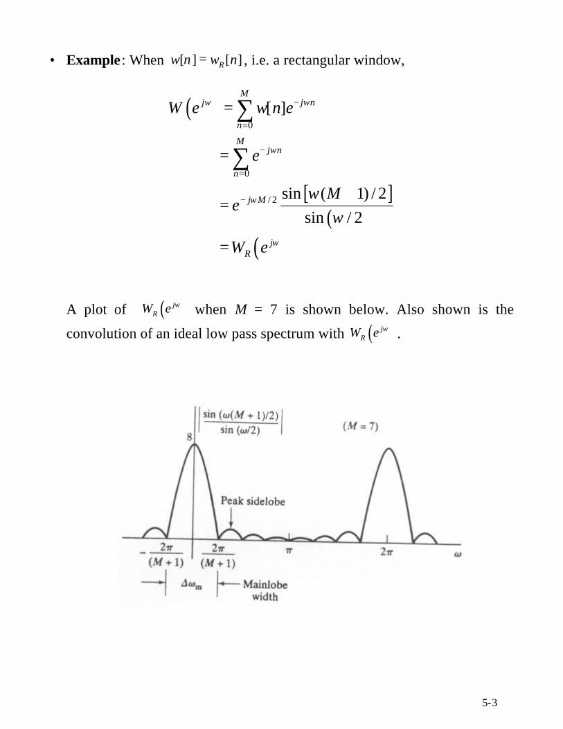
A plot of ( )jRW e ω when M = 7 is shown below. Also shown is the

convolution of an ideal low pass spectrum with ( )jRW e ω .

5-4

• The convolution in the frequency domain leads to a smearing of thespectrum. The sinusoidal nature of the sinc function in ( )j

RW e ω leads to

the oscillations in ( )jH e ω - the Gibbs phenomenon.

• To reduce the smearing and oscillations, we should use a windowingfunction whose ( )jW e ω has a (relatively)

1. narrow mainlobe, and2. low sidelobes

Note that

5-5

1. the longer the windowing function (in the time domain), the narroweris the main lobe, and

2. the “smoother” the windowing function (in the time domain), thelower the sidelobes.

It is clear that when M is fixed, we have conflicting requirements.

• Raised Cosine family of windows

Many commonly used windowing functions can be written in the generalform

2 4[ ] cos cos ; 0

n nw n a b c n M

M M

π π = + + ≤ ≤ .

(a) Rectangular window

1, 0 , 0a b c= = =

(b) Hanning window

0.5, 0.5, 0a b c= = − =

(c) Hamming window

0.54, 0.46, 0a b c= = − =

(d) Blackman window

0.42, 0.5, 0.08a b c= = − =

5-6

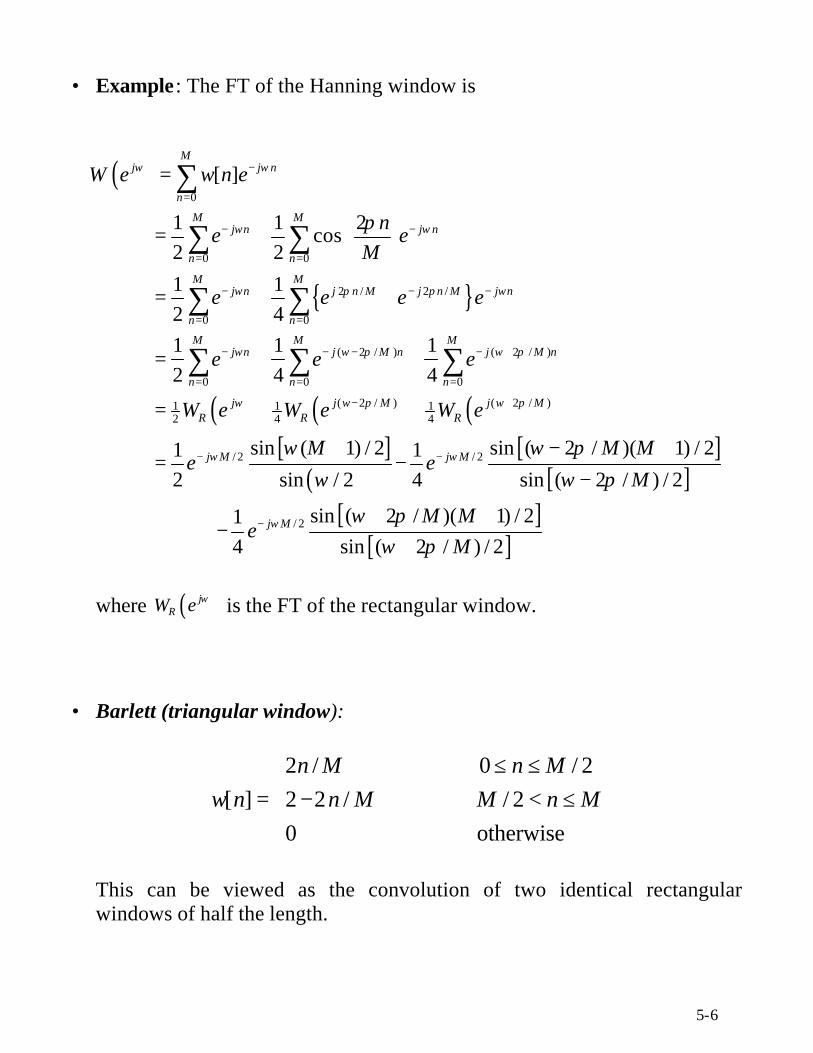
• Example : The FT of the Hanning window is

( )

0

0 0

2 / 2 /

0 0

( 2 / ) ( 2 / )

0 0 0

12

[ ]

1 1 2 cos

2 2

1 1

2 41 1 1

2 4 4

Mj j n

n

M Mj n j n

n n

M Mj n j n M j n M j n

n n

M M Mj n j M n j M n

n n n

W e w n e

ne e

M

e e e e

e e e

ω ω

ω ω

ω π π ω

ω ω π ω π

π

−

=

− −

= =

− − −

= =

− − − − +

= = =

=

= +

= + +

= + +

=

∑

∑ ∑

∑ ∑

∑ ∑ ∑( ) ( ) ( )

[ ]( )

[ ][ ]

[ ][ ]

( 2 / ) ( 2 / )1 14 4

/ 2 / 2

/ 2

sin ( 1) / 2 sin ( 2 / )( 1) / 21 1

2 sin / 2 4 sin ( 2 / ) / 2

sin ( 2 / )( 1) / 21

4 sin ( 2 / ) / 2

j j M j MR R R

j M j M

j M

W e W e W e

M M Me e

M

M Me

M

ω ω π ω π

ω ω

ω

ω ω π

ω ω π

ω πω π

− +

− −

−

+ +

+ − += −

−

+ +−

+

where ( )jRW e ω is the FT of the rectangular window.

• Barlett (triangular window):

2 / 0 / 2[ ] 2 2 / / 2

0 otherwise

n M n M

w n n M M n M

≤ ≤= − < ≤

This can be viewed as the convolution of two identical rectangularwindows of half the length.

5-7

• Plot of different windowing functions in the time domain

• The spectral characteristics of the different windows are shown in the nexttwo pages. Numerical values of the peak sidelobe and width of the mainlobe are summarized below.

5-8

(a) Rectangular window, (b) Barlett window, (c) Hanning window

5-9

(d) Hamming window, (e) Blackman window

• The spectrum of the rectangular window is characterised by a relativelynarrow main lobe but high sidelobes and a slow rate of decay.

• The triangular window is the convolution of 2 rectangular windows of halfthe size. This means

5-10

1. the spectrum of a triangular window has a 2sinc characteristics, i.e. itdecays asymptotically at twice the rate of the spectrum of a rectangularwindow;

2. the width of the mainlobe and sidelobes are twice that in the spectrum ofa rectangular window (because of the “halfing” in the time domain).

• Recall that the spectrum of the Hanning window is the sum of 3 differentfrequency shifted versions of ( )j

RW e ω , the spectrum of a rectangularwindow. Consequently it has a wider main lobe.

Since this windowing function tapers off to zero very smoothly, it hasmuch lower sidelobes than the rectangular window.

• The main lobe width of the Hamming window is similar to that of theHanning window for exactly the same reason.

The sidelobes, although lower than that of the rectangular window, decaysvery slowly. This is due to the discontinuities at the two edges of thewindow.

• The spectral mainlobe of the Blackman window is wider than that of theHamming/Hanning windows because of the additional cosine term in thewindowing function.

Its sidelobes, however, are lower because of the smoother transition tozero.

5-11

• All the windows described above have the property that

[ ] 0[ ]

0 otherwise

w M n n Mw n

− ≤ ≤=

.

This means (assuming M is even)

( )

( )

0

/ 2 1( ) / 2

0

/ 2 1/ 2 ( / 2 ) ( / 2 ) / 2

0

/ 2 1/ 2 / 2

20

[ ]

[ ] [ /2]

[ ] [ /2]

2 [ ]cos [ /2]

Mj j n

n

Mj n j M n j M

n

Mj M j M n j M n j M

n

Mj M j MM

n

W e w n e

w n e e w M e

e w n e e w M e

e w n n w M e

ω ω

ω ω ω

ω ω ω ω

ω ωω

−

=

−− − − −

=

−− − − − −

=

−− −

=

=

= + +

= + +

= − +

∑

∑

∑

∑

( )

( )

/ 2 1/ 2

20

/ 2

[ /2 ] 2 [ ]cos

Mj M M

n

j M je

e w M w n n

e W e

ω

ω ω

ω−

−

=

−

= + − =

∑

where

( ) ( )/ 2 1

20

[ / 2] 2 [ ]cosM

j Me

n

W e w M w n nω ω−

=

= + − ∑

is a real and even function in ω .

Note that the phase of ( )jW e ω is linear.

In most design exercises, we can ignore the phase and focus only on( )j

eW e ω .

5-12

• If the desired impulse response is of linear phase, i.e.

[ ] [ ]d dh n h M n= − ,

then

( ) ( ) / 2j j j Md eH e H e eω ω ω−=

where ( )jeH e ω is a real and even function in ω .

• Exercise: Shown that if both [ ]w n and [ ]dh n are linear phase, then

[ ] [ ] [ ]dh n h n w n=

is also linear phase, i.e.

( ) ( ) / 2j j j MeH e A e eω ω ω−=

where ( )jeA e ω is a real and even function in ω . Consequently during filter

design, we can just focus on ( )jeA e ω and ( )j

eH e ω .

5.1.1 Kaiser Windows

• All the windows discussed so far can be approximated by an equivalentKaiser window of the form

5-13

( )( )

20

0

1 0[ ]

0 otherwise

nIn Mw n I

ααβ

β

− − ≤ ≤=

,

where2

cos0

0

1( )

2xI x e d

πθ θ

π= ∫

is the modified zero-th order Bessel function of the first kind,

/ 2Mα =

is half the window length, and β is a design parameter.

• Let the square-root term inside one of the bessel functions be denoted by

5-14

2

1n

nx

αα− = − .

As shown in the figure below, nx increases monotonically from 0 to 1 inthe interval 0 n α≤ ≤ and decreases monotonically from 1 to 0 in theinterval n Mα ≤ ≤ . Consequently, [ ]w n is largest at n α= but decreasesmonotonically on ether sides of this maxima.

When 0β = , [ ] 1w n = for all values of n. In other word, the Kaiser windowat this value of β degenerates into a rectangular window.

5-15

• Plot of Kaiser windows in the time and frequency domains.

5-16

It is observed that:

1. the Kaiser windows have linear phase, and2. the larger β is, the smoother is the windowing function. This implies a

wider mainlobe but lower sidelobes.

The relationships between Kaiser windows and other windows are shownin the table on pp 2-7.

• Design guidelines using Kaiser windows

- Assume a low pass filter .

- Given that Kaiser windows have linear phase, we will only focus on thefunction ( )j

eA e ω in the approximation filter ( )jH e ω and the term

( )jeH e ω in the ideal low pass filter ( )j

dH e ω .

- Normalize ( )jeH e ω to unity for 0 cω ω≤ ≤ , where cω is the cutoff

frequency of the ideal low pass filter.

- Specify ( )jeA e ω in terms of a passband frequency pω , a stop band

frequency sω , a maximum passband distortion of 1δ , and a maximum

stopband distortion of 2δ . Note that (1) the cutoff frequency cω of theideal low pass filter is midway between pω and sω , (2) 1δ should equalto 2δ because of the nature of windowing.

5-17

- Let

s pω ω ω∆ = − ,

1 2δ δ δ= = ,and

1020logA δ= − .

Then choose β and M according to

0.4

0.1102( 8.7) 500.5842( 21) 0.07886( 21) 21 500 <21

A A

A A A

A

β− >

= − + − ≤ ≤

and8

2.285A

Mω

−=

∆

5-18

• Example : Determine cω , β , and M when 0.4pω π= , 0.6sω π= , and

1 2 0.001δ δ δ= = = .

Solution:

Since 1020log 60A δ= − = , this means

0.1102(60 8.7) 5.6533β = − = .

Since 0.2s pω ω ω π∆ = − = and 60A = ,

60 836.22 37

2.285 0.2M

π−

= = →×

• Example : Consider an ideal bandpass filter with a frequency response

( )/2 0.3 0.7

0 otherwise

j Mj

d

eH e

ωω π ω π− ≤ ≤

=

The corresponding impulse response, [ ]dh n , is symmetrical about/ 2 25.Mα = = We want to approximate this ideal filter by multiplying it

with a Kaiser window of length 1 51M + = and with 3.9754β = . Determinethe width of the transition bands ω∆ and the maximum distortion δ . Whatare the passband and stopband frequencies?

Solution:

- Since the length of the window is 1M + and [ ]dh n is symmetrical about/ 2M , the approximation filter ( )jH e ω has linear phase and can be

rewritten in the form ( ) ( ) /2j j j MeH e A e eω ω ω−= , where ( )j

eA e ω is a real and

5-19

even function in ω . Consequently we can just focus on the term ( )jeA e ω

and have the following specifications:

- In the time domain, the desired impulse response is

( ) ( )sin 0.7 ( 25) sin 0.3 ( 25)[ ]

( 25) ( 25)d

n nh n

n n

π π

π π

− −= −

− − ,

which is the difference of two ideal low pass signals.

- When the Kaiser window is applied to any of the two low passcomponents of [ ]dh n , there is a peak spectral distortion of λ . So thetotal spectral distortion is 2δ λ= (a conservative estimate).

- Given 3.9754β = , it means 1020log 45A λ= − = , or 35.6234 10λ −= × .Consequently

22 1.3247 10δ λ −= = × .

( )jeA e ω

1 δ+

δ−

δ

1

0.3π 0.7π

ω

1 δ+

5-20

- The width of each of the two transition bands in ( )jeA e ω is governed by

80.1031

2.285A

Mω π

−∆ = =

This means the stopband frequencies are

1

2

0.3 0.1031 / 2 0.2485

0.7 0.1031 / 2 0.7516

s

s

ω π π π

ω π π π

= − =

= + =

and the passband frequencies are

1

2

0.3 0.1031 / 2 0.3516

0.7 0.1031 / 2 0.6485

p

p

ω π π π

ω π π π

= + =

= − =

• In general, any ideal multiband filter can be expressed as a weighted sumof ideal low pass signals of different frequencies, i.e.

( )/ 2

1

sin ( /2)[ ]

( /2)

Nkj M

d kk

n Mh n e w

n Mω ω

π−

=

−=

−∑

with real weight coefficients kw . The total distortion is

1

N

kk

wδ λ=

= ∑

where λ is the peak distortion when the Kaiser window is applied to eachindividual ideal low pass signal.

5-21

5.2 The Park-McClellan Algorithm

• The windowing method of FIR filter design is straight forward. However,the technique has 2 disadvantages:

1. distortion in the passband and the stopband are more or less equal, and2. distortion is usually largest at the discontinuities of the ideal frequency

response.

• Very often, we want to design a filter with different passband and stopbanddistortions.

In addition, if the distortion is more evenly spread, we will be able to comeup with a shorter FIR filter.

• The Park-McClellan algorithm is an iterative procedure for designing anequi-ripple FIR filter with different distortion in the pass and stop bands.

We will focus our attention on the design of low pass filters of length

2M L=using this method.

The design of low pass filters with an odd value of M, as well as the designof other types of filters (such as bandpass, highpass, etc), require somemodifications to the procedure to be described.

5-22

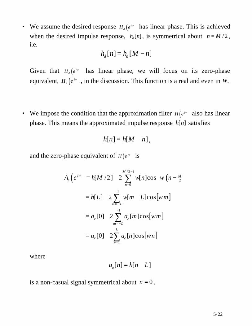
• We assume the desired response ( )jdH e ω has linear phase. This is achieved

when the desired impulse response, [ ]dh n , is symmetrical about / 2n M= ,i.e.

[ ] [ ]d dh n h M n= −

Given that ( )jdH e ω has linear phase, we will focus on its zero-phase

equivalent, ( )jeH e ω , in the discussion. This function is a real and even in ω.

• We impose the condition that the approximation filter ( )jH e ω also has linearphase. This means the approximated impulse response [ ]h n satisfies

[ ] [ ]h n h M n= − ,

and the zero-phase equivalent of ( )jH e ω is

( ) ( )

[ ]

[ ]

[ ]

/ 2 1

20

1

1

1

[ /2] 2 [ ]cos

[ ] 2 [ ]cos

[0] 2 [ ]cos

[0] 2 [ ]cos

Mj M

en

m L

e em L

L

e en

A e h M w n n

h L w m L m

a a m m

a a n n

ω ω

ω

ω

ω

−

=

−

=−

−

=−

=

= + −

= + +

= +

= +

∑

∑

∑

∑

where[ ] [ ]ea n h n L= +

is a non-casual signal symmetrical about 0n = .

5-23

• The term ( )cos nω can be written as a polynomial of degree n in ( )cos ω .

For example, ( ) ( )2cos 2 2cos 1ω ω= − , and ( ) ( ) ( )3cos 3 4cos 3cosω ω ω= − , etc.

This means the zero-phase response ( )jeA e ω can be written as a L-th order

polynomial in ( )cos ω :

( ) ( )0

cos( )L

kje k

k

A e aω ω=

= ∑

where the ka s are the coefficients in this polynomial respresention.

• The Park-McCelland algorithm allows us to find the optimal ( )jeA e ω (i.e.

the coefficients ka in the polynomial representation) for fixed L, pω , sω ,and

1

2

Kδδ

= .

The distortion, 1δ (or 2δ ), however is a variable. Let us define theapproximation error function as

( ) ( ) ( ) ( ) j je eE W H e A eω ωω ω= − ,

where

( ) 1/ 01

p

s

KW

ω ωω

ω ω π≤ ≤

= ≤ ≤

is a weighting function that normalizes the spectral distortion in the passand stop bands. (notice that the weighting function is not defined fortransition band, i.e. when p sω ω ω≤ ≤ ).

5-24

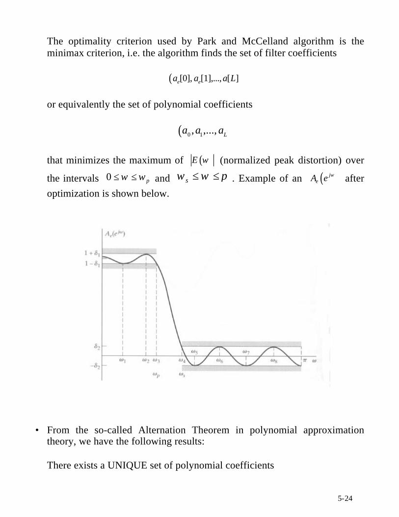
The optimality criterion used by Park and McCelland algorithm is theminimax criterion, i.e. the algorithm finds the set of filter coefficients

( )[0], [1],..., [ ]e ea a a L

or equivalently the set of polynomial coefficients

( )0 1, ,..., La a a

that minimizes the maximum of ( )E ω (normalized peak distortion) over

the intervals 0 pω ω≤ ≤ and sω ω π≤ ≤ . Example of an ( )jeA e ω after

optimization is shown below.

• From the so-called Alternation Theorem in polynomial approximationtheory, we have the following results:

There exists a UNIQUE set of polynomial coefficients

5-25

( )0 1, ,..., La a a

and a unique set of extremal frequencies

1 2 2, ,..., Lω ω ω +Ω = ,with

1 2 2Lω ω ω +< < <L ,such that

( ) ( ) 11 i

iE ω δ+= − (equiripple)

where δ is the minimum peak distortion. Note that both the pass bandfrequency pω and the stop band frequency sω belong to Ω , and if

k pω ω= ,then

1k sω ω+ = .

• The Park-McClelland algorithm uses an iterative procedure to find the setof extremal frequencies.

1. At the start of the algorithm, guess the the locations of the L+2 extremalfrequencies. Call these frequencies ˆ ; 1,2,..., 2k k Lω = + .

2. Define kx as

( )ˆcosk kx ω=

3. Use (7.101) and (7.102) to obtain δ , an estimate of the normalized peakdistortion δ .

5-26

4. Use (7.103) to compute ( )ˆ jeA e ω , an estimate of ( )j

eA e ω . This functionhas the characteristics

( )ˆ1 / ˆ

ˆ k k pj

e

k s

KA e ω δ ω ω

δ ω ω

± ≤= ± ≥

.

5. Locate the local maxima in

( ) ( ) ( ) ˆˆ ( ) j je eE W H e A eω ωω ω= −

where ˆˆ( )E ω δ≥ . If there are more than 2L + such maxima ( pω and sω

are counted as “maxima” even though the slopes at these twofrequencies are not zero), retain only the 2L + largest ones. Call thesefrequencies ; 1,2,..., 2k k Lω = +% .

5-27

6. If the kω% s differ “substantianlly” from the ˆ kω s, update the ˆ kω s usingthese frequencies and go back to Step 2. If not, declare that the optimal

solution has been found. In this case, make ˆk kω ω= , ˆδ δ= , and

( ) ( )ˆj je eA e A eω ω= . Take a M-point IFFT of ( )j

eA e ω to obtain [ ]ea n .

Delay [ ]ea n by / 2L M= samples to obtain [ ]h n .

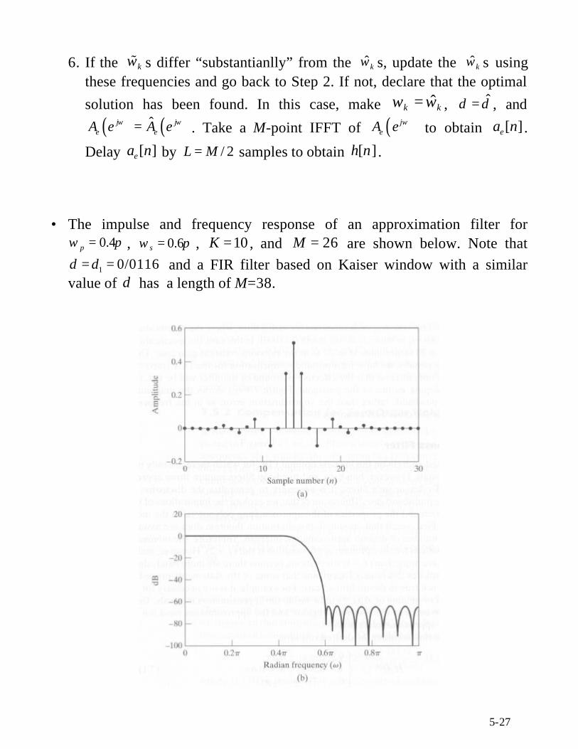
• The impulse and frequency response of an approximation filter for0.4pω π= , 0.6sω π= , 10K = , and 26M = are shown below. Note that

1 0/0116δ δ= = and a FIR filter based on Kaiser window with a similarvalue of δ has a length of M=38.

5-28

5.3 Implementation Structure of FIR Filters

• Reference: Section 6.5 of Text

• The relationship between the input [ ]x n and the output [ ]y n of a FIR filterof length 1M + is

0

[ ] [ ] [ ]M

k

y n h k x n k=

= −∑ ,

where [ ]h n is the impulse response of the filter, and

0

( ) [ ]M

k

k

H z h k z−

=

= ∑

is the transfer function of the filter.

• According to the above equations, a possible implementation structure ofthe FIR filter is

5-29

This is called the direct form implementation. Note that a branch in thesignal flow graph with a transmittance of 1z− represents a delay of 1sample. On the other hand, a branch with a transmittance of [ ]h k means thesignal at the originating node of that branch is multiplied by the constant

[ ]h k . Again, as in any signal flow graph, the signal at a node is the sum ofthe product of the signal at an originating node and the correspondingbranch transmittance.

• The transfer function ( )H z of a FIR filter can be expressed in terms of itszeros according to the following equation

( ) ( )( )1 2

1 1 * 1

1 1

( ) 1 1 1M M

k k kk k

H z C f z g z g z− − −

= =

= − − −∏ ∏

Here the kf ’s are the real zeros and the kg ’s are the complex zeros. Theparameter C is a constant.

The complex zeros will always appear in conjugate pairs (as long as the

impulse response is real). Moreover, ( ) ( )1 * 11 1k kg z g z− −− − is a 2nd order

polynoimal in 1z − with real coefficients.

Assuming 1 2M K= , where K is an integer. Then we can group the11 kf z −− ’s into pairs and the product of any pair is always a 2nd order

polynoimal in 1z − with real coefficients. In other word, the transferfunction can always be written in product form as

( ) ( )1 20 1 2

1 1

( ),s sM M

k k k kk k

H z b b z b z B z− −

= =

= + + =∏ ∏where

5-30

( )1 20 1 2( )k k k kB z b b z b z− −= + +

and

2sM K M= + .

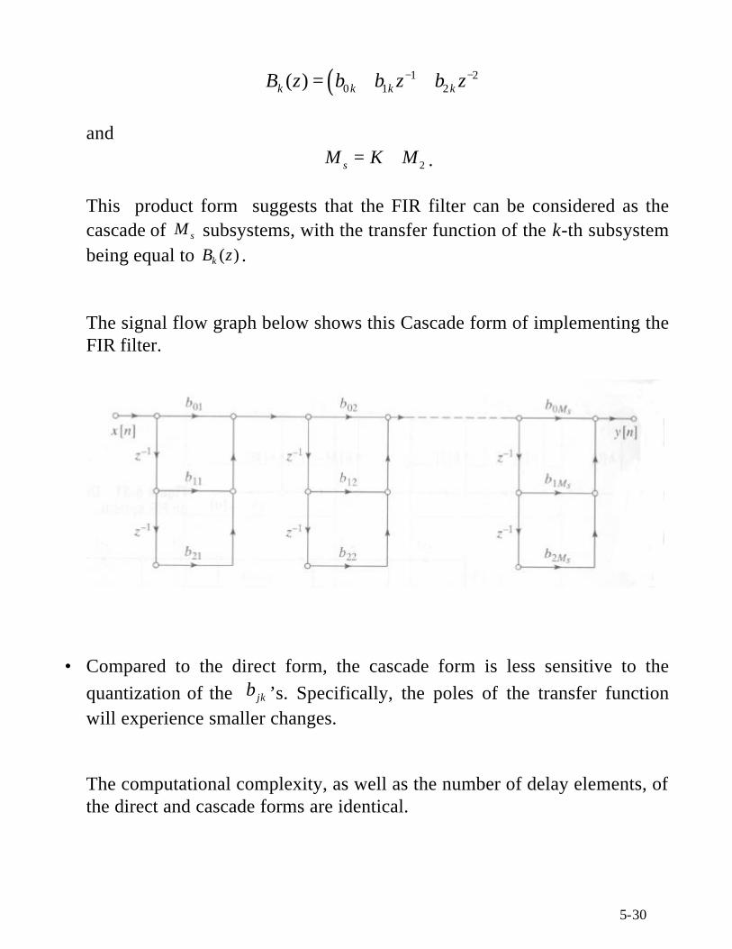
This product form suggests that the FIR filter can be considered as thecascade of sM subsystems, with the transfer function of the k-th subsystembeing equal to ( )kB z .

The signal flow graph below shows this Cascade form of implementing theFIR filter.

• Compared to the direct form, the cascade form is less sensitive to thequantization of the jkb ’s. Specifically, the poles of the transfer functionwill experience smaller changes.

The computational complexity, as well as the number of delay elements, ofthe direct and cascade forms are identical.

5-31

• All the FIR filters considered in this chapter are assumed to have linearphase. This is a direct result of the symmetry in the impulse response.Specifically

[ ] [ ]; 0,1,...,h M n h n n M− = =

Because of the symmetry, there is no need to do all the 1M +multiplications in the direct form implementation of the FIR filter. We canfirst add [ ]x n k− and [ ]x n k M+ − together before multiplying the sumby [ ]h k . The figure below illustrates the direct form structure for a FIRlinear phase system when M is an even integer.

• It is also possible to implement a linear phase FIR filter, with reducedcomplexity, using the cascade form.