Embed Size (px)
Citation preview

Chapter 7 Filter Design Techniques
Introduction
Design of FIR Filters by Windowing
Examples of FIR Filter Design by the Kaiser Window
Method
Design of Discrete-Time IIR Filters from Continuous-Time
Filters
Frequency Transformations of Lowpass IIR Filters
Appendix Continuous Filters

1. Introduction
Filters
Frequency-selective Filter
Three Stages
Specifications
Approximation of the Spec.
Realization
Ex.
Spec.
Linear Phase ?

2. Design of FIR Filters by Windowing
Procedure
Desired Frequency Response
Corresponding Impulse Response
Length is Infinity
Truncation
H e h n edj
dj n
n
( ) [ ]
h n H e e dd dj j[ ] ( )
1
2
h nh n n M
otherwised[ ][ ],
,
0
0

2. Design of FIR Filters by Windowing
(c.1)
Analysis
Windowing in Time
Convolution in Frequency
Points
Width of the Mainlobe
Attenuation of the Sidelobe
h n h n w n
where
w nn M
otherwise
d[ ] [ ] [ ]
[ ],
,
1 0
0
H e H e W e djd
j j( ) ( ) ( )( )
1
2
Rect. Window
Freq. Resp.
Convolution
Results

2. Design of FIR Filters by Windowing
(c.2)
Properties of Commonly Used Windows

2. Design of FIR Filters by Windowing
(c.3)
Properties of
Commonly Used
Windows (c.1)

2. Design of FIR Filters by Windowing
(c.4)
Generalized Linear Phase
Symmetric of the Windowing
w nw M n n M
otherwise( )
( ),
,
0
0

2. Design of FIR Filters by Windowing
(c.5)
The Kaiser Window Filter
Zeroth-order Bessel Function of
the First Kind
Two Parameters
a and b
w nI n
In M
otherwise
( )[ ( [( )/ ] ) ]
( ),
,
/
02 1 2
0
10
0
b a a
b
a M /2

Bessel function
Defined by the mathematician Daniel Bernoulli and generalized by
Friedrich Bessel, are canonical solutions y(x) of Bessel's differential
equation.

2. Design of FIR Filters by Windowing
(c.6)
The Kaiser Window Filter -- Procedure
Evaluate first the two values
Value of b (empirically) and M
Example
s p
A 20 10log
MA
8
2 285.
p
s
0 4
0 6
0 01
0 001
1
2
.
.
.
.
0 2
0 001
.
.
b
5 653
37
.
M
h nn
n
I n
In M
otherwise
c
[ ]sin ( )
( )
[ ( [( )/ ] ) ]
( ),
,
/
a
a
b a a
b0
2 1 2
0
10
0

3. Examples of FIR Filter Design by the
Kaiser Window Method
Highpass Filter
Freq. Resp.
Impulse Response
Impulse Response of the High pass Filters
Generalized Multiband Filters
c
Mj
cj
hpe
eH,
0,0)(
2/
H e e H ehpj j M
lpj( ) ( )/ 2
h nn M
n M
n M
n Mnhp
c[ ]sin ( / )
( / )
sin ( / )
( / ),
2
2
2
2
h n G Gn M
n Mnmb k k
k
k
N mb
[ ] ( )sin ( / )
( / ),
1
1
2
2

4. Design of Discrete-Time IIR Filters
from Continuous-Time Filters
Motivation for Digital Filter from Analog Filter
Analog IIR filter design is highly advanced.
Have relatively simple closed form design
The methods do not lead to a simple closed form design formulas
for discrete-time IIR case.
Analog Filters
An analog filter may be described as
Analog filter is stable if all its poles lie in the left-half of s-plane.
The jW axis in the s-plane ==> the unit circle in the z-plane.
The left-half plane of the s-plane ==> Inside the unit circle.
H sB s
A s
s
sa
kk
k
M
kk
k
N( )
( )
( )
b
a
0
0

4. Design of Discrete-Time IIR Filters from Continuous-Time
Filters-- Filter Design by Impulse Invariance
Concepts
The sampling of Impulse response
h[n] = Thc(nT)
Freq. Relation
Ex.
H e H jTjTkj
ck
( ) ( )
2 Aliasing
H sA
s sck
kk
N
( )
1
h tA e t
tc
ks t
k
Nk
( ),
,
0
0 01
h n Th nT TAe u n TA e u ncs nT
k
Ns T n
k
Nk d k[ ] ( ) [ ] [ ]
1 1
H zTA
e zks T
k
N
k( )
1 11
z e sT
•The mapping is not one-to-one.
•The selection of T to minimize the aliasing.
•Appropriate for low-pass and band-pass filters.

4. Design of Discrete-Time IIR Filters from Continuous-
Time Filters-- Bilinear Transformation
Concepts
Formula
Frequency Relation
Frequency mapping
or
sT
z
z
H z HT
z
zc
2 1
1
2 1
1
1
1
1
1( )
zT s
T s
1 2
1 2
( / )
( / )e
T j
T jj
1 2
1 2
( / )
( / )
W
W
s jT
e j
e
j
T
j
j
W2 2 2
2 2
22
2
2
/
/
( sin / )
( cos / )tan( / )
W
2 2 2
2 2
22
2
2T
e j
e T
j
j
/
/
( sin / )
( cos / )tan( / )
2 2arctan( / )WT
2/)2/(1
2/)2/(1
TjT
TjTz
W
W

5. Frequency Transformations of
Lowpass IIR Filters
Transform
Replacing the variable z-1 by a rational
function
z-1 = g(z-1)
Conditions
Unit circle to unit circle.
Inside unit circle to Inside unit circle.
Form
e g e g
g e
j j
j g
( ) ( )
( )arg ( )
g zz
zk
kk
n
( )
1
1
11 1
a
a
ak 1 ensures the stable filter is transformed
into another stable system
Transform from lowpass digital filter prototype cutoff
frequency .

6. Concluding Remarks
Introduction
Design of FIR Filters by Windowing
Examples of FIR Filter Design by the Kaiser Window
Method
Design of Discrete-Time IIR Filters from Continuous-Time
Filters
Frequency Transformations of Lowpass IIR Filters

Continuous-Time Filters
C.M. Liu
Perceptual Signal Processing Lab
College of Computer Science
National Chiao-Tung University
Office: EC538
(03)5731877
(
http://www.csie.nctu.edu.tw/~cmliu/Courses/DSP/

Contents
Butterworth Lowpass Filters
Chebyshev Filters
Elliptic Filters
18
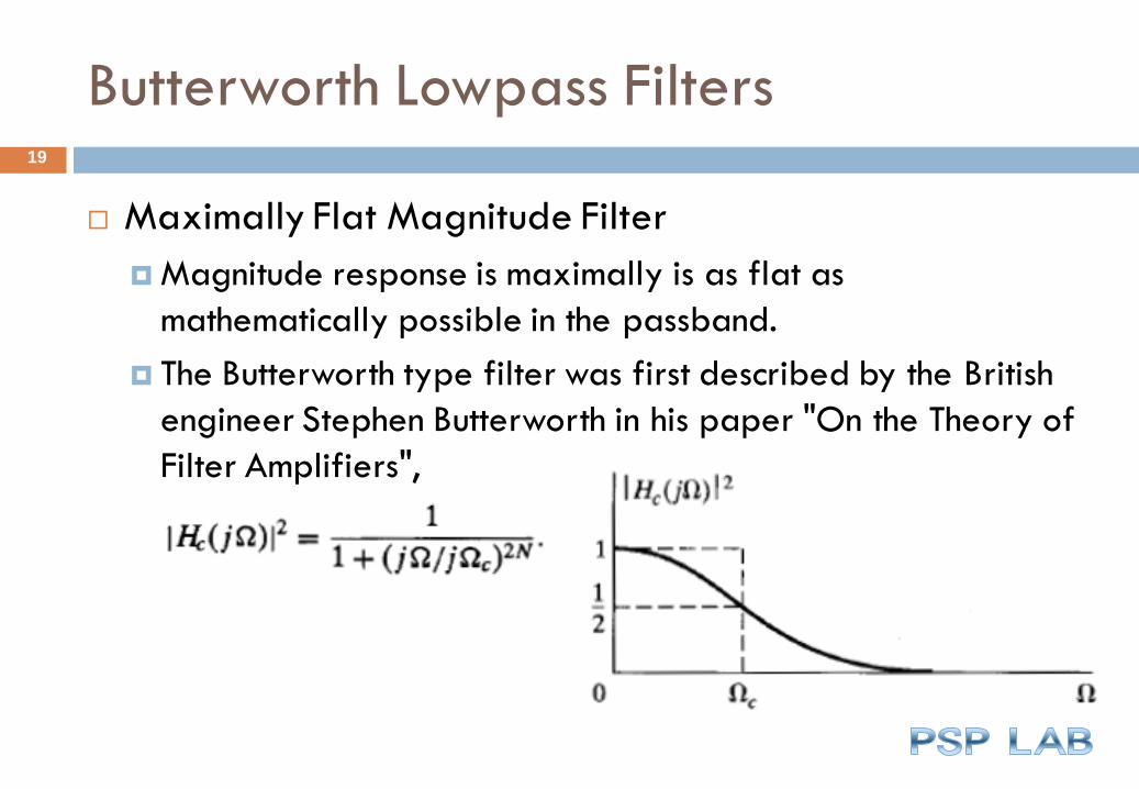
Butterworth Lowpass Filters
Maximally Flat Magnitude Filter
Magnitude response is maximally is as flat as
mathematically possible in the passband.
The Butterworth type filter was first described by the British
engineer Stephen Butterworth in his paper "On the Theory of
Filter Amplifiers",
19

Butterworth Lowpass Filters
Let
20
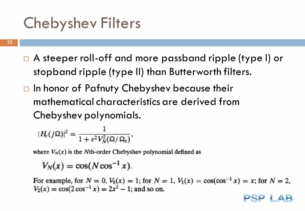
Chebyshev Filters
A steeper roll-off and more passband ripple (type I) or
stopband ripple (type II) than Butterworth filters.
In honor of Pafnuty Chebyshev because their
mathematical characteristics are derived from
Chebyshev polynomials.
21

Chebyshev Filters22

Chebyshev Filters
Type II is related Type I through
a transformation
23
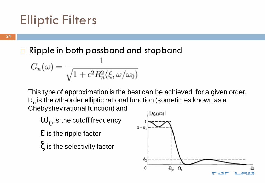
Elliptic Filters
Ripple in both passband and stopband
24
This type of approximation is the best can be achieved for a given order.
Rn is the nth-order elliptic rational function (sometimes known as a
Chebyshev rational function) and
ω0 is the cutoff frequency
ε is the ripple factor
ξ is the selectivity factor

Homeworks
7.6; 7.15; 7.16; 7.27; 7.31;