5. Coupling of Chemical Kinetics & Thermodynamicsarrow.utias.utoronto.ca/~ogulder/ClassNotes5.pdf · • Using definition of enthalpy h ≡u + Pv,and differentiating ... • Also

5. Coupling of Chemical Kinetics &Thermodynamics

Objectives of this section:• Thermodynamics: Initial and final states are con-sidered:- Adiabatic flame temperature- Equilibrium composition of products- No knowledge of chemical rate processesrequired

5. Coupling of Kinetics & Thermodynamics 1 AER 1304–ÖLG

Objectives of this section (Cont’d):• In this section aim is to couple thermodynamicswith chemical rate processes.

• Follow the system temperature and the variousspecies concentrations as functions of time as thesystem moves from reactants to products.

• Systems chosen to demonsrate the basic conceptswill be simple with bold assumptions.

• Interrelationship among thermodynamics, chemicalkinetics, and fluid mechanics.


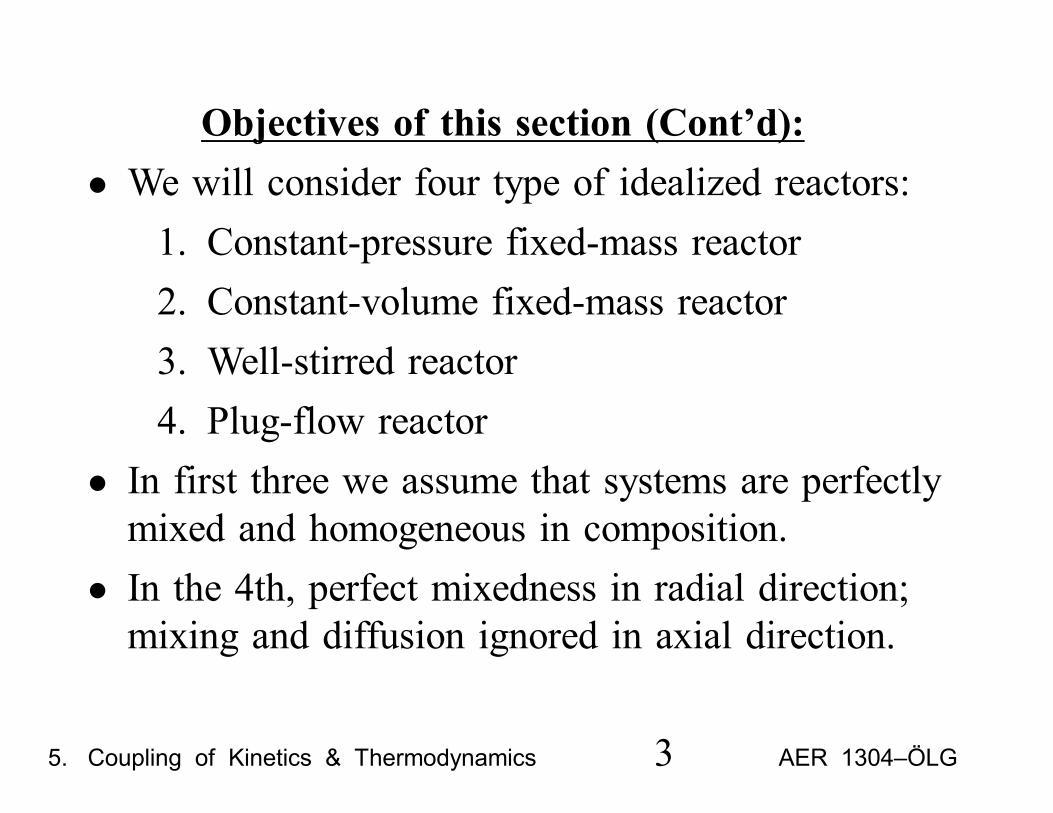
Objectives of this section (Cont’d):• We will consider four type of idealized reactors:

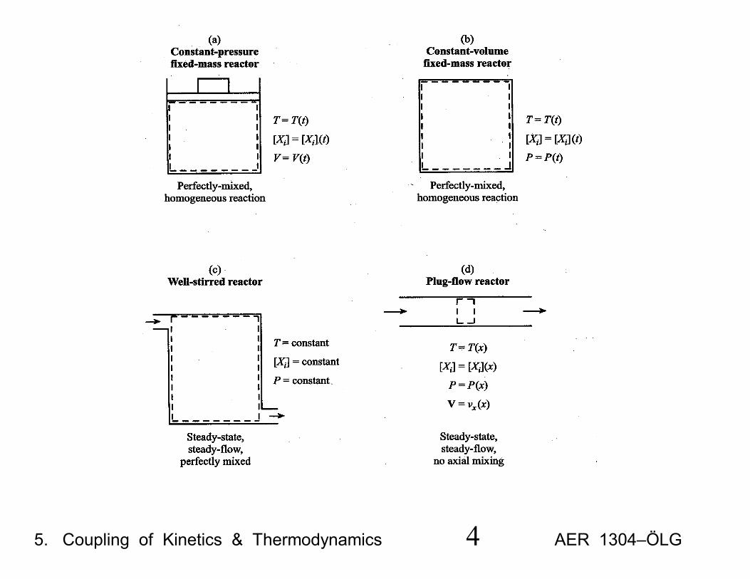
1. Constant-pressure fixed-mass reactor2. Constant-volume fixed-mass reactor3. Well-stirred reactor4. Plug-flow reactor

• In first three we assume that systems are perfectlymixed and homogeneous in composition.

• In the 4th, perfect mixedness in radial direction;mixing and diffusion ignored in axial direction.



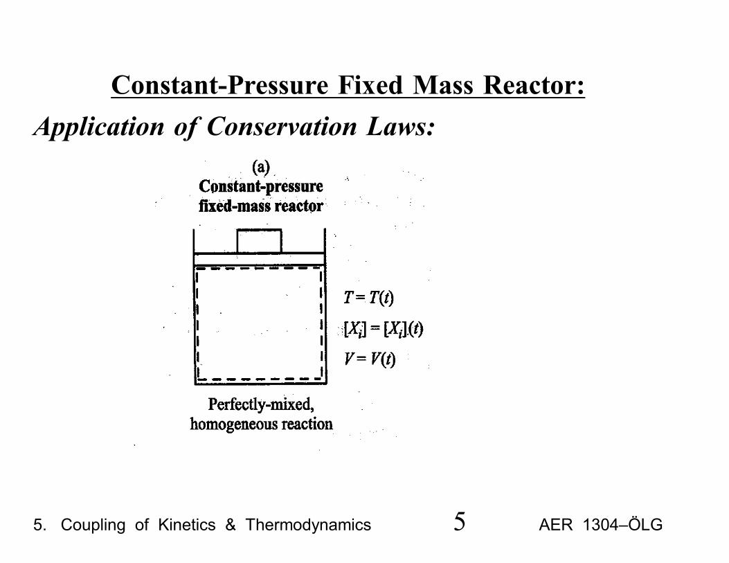
Constant-Pressure Fixed Mass Reactor:Application of Conservation Laws:


• Reactants react at each and every location withinthe volume at the same time.

• No temperature or composition gradients withinthe mixture.

• Single temperature and a set of species concentra-tions are sufficient to describe the evolution of thesystem.

• For combustion reactions, both temperature andvolume will increase with time.

• There may be heat transfer through the reactionvessel walls.


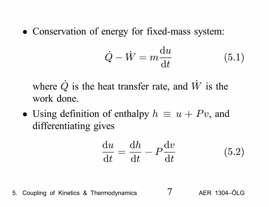
• Conservation of energy for fixed-mass system:

Q− W = mdu

dt(5.1)

where Q is the heat transfer rate, and W is thework done.

• Using definition of enthalpy h ≡ u + Pv, anddifferentiating gives

du

dt=dh

dt− P dv

dt(5.2)


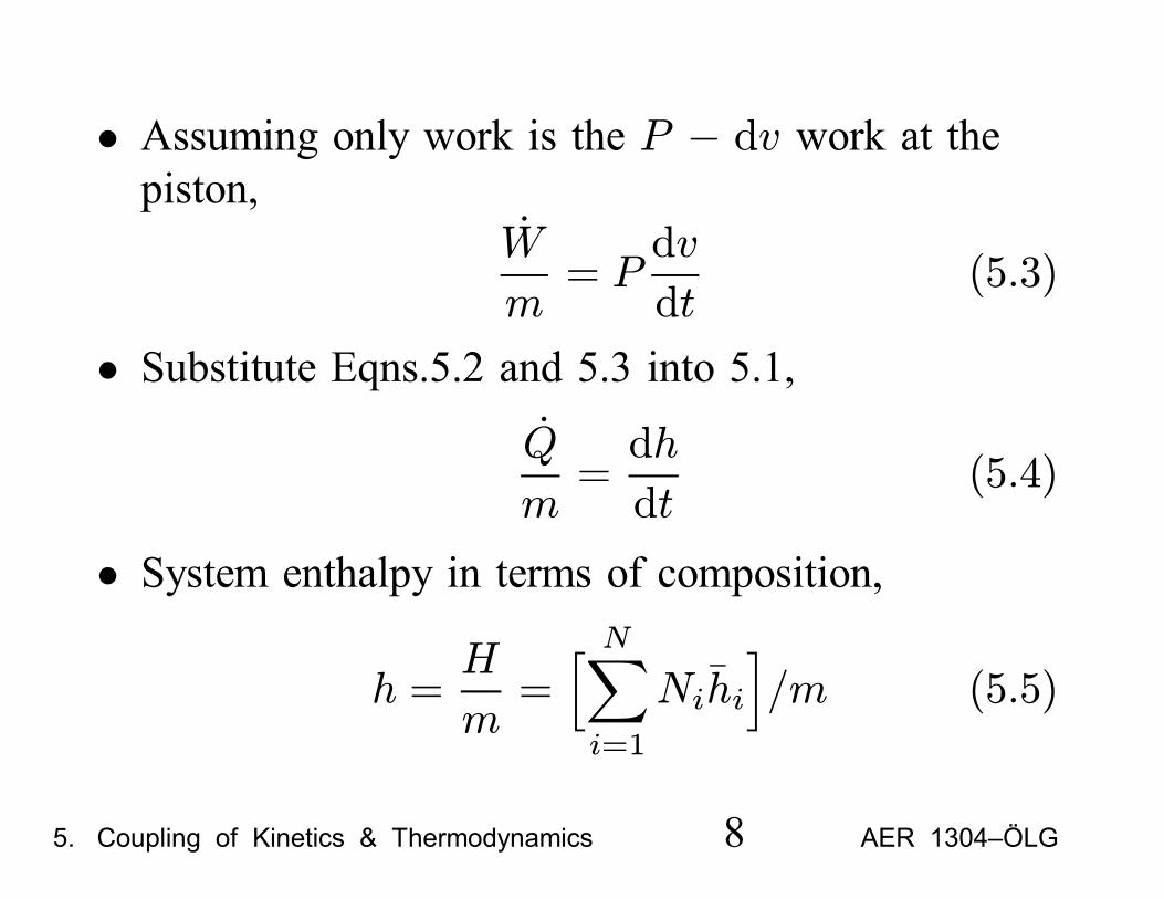
• Assuming only work is the P − dv work at thepiston,

W

m= P

dv

dt(5.3)

• Substitute Eqns.5.2 and 5.3 into 5.1,Q

m=dh

dt(5.4)

• System enthalpy in terms of composition,

h =H

m=

N

i=1

Nihi /m (5.5)


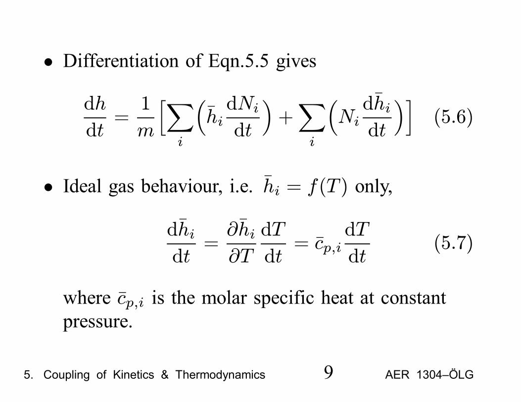
• Differentiation of Eqn.5.5 givesdh

dt=1

mi

hidNidt

+i

Nidhidt

(5.6)

• Ideal gas behaviour, i.e. hi = f(T ) only,

dhidt

=∂hi∂T

dT

dt= cp,i

dT

dt(5.7)

where cp,i is the molar specific heat at constantpressure.


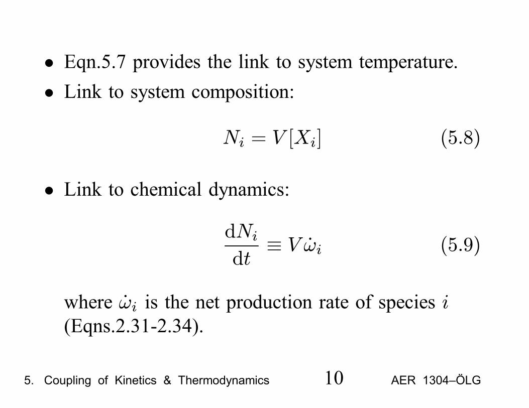
• Eqn.5.7 provides the link to system temperature.• Link to system composition:

Ni = V [Xi] (5.8)

• Link to chemical dynamics:dNidt≡ V ωi (5.9)

where ωi is the net production rate of species i(Eqns.2.31-2.34).


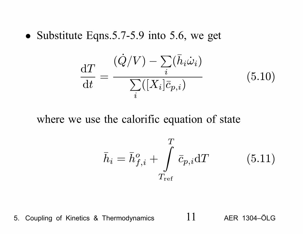
• Substitute Eqns.5.7-5.9 into 5.6, we get

dT

dt=

(Q/V )−i

(hiωi)

i

([Xi]cp,i)(5.10)

where we use the calorific equation of state

hi = hof,i +

T

Tref

cp,idT (5.11)


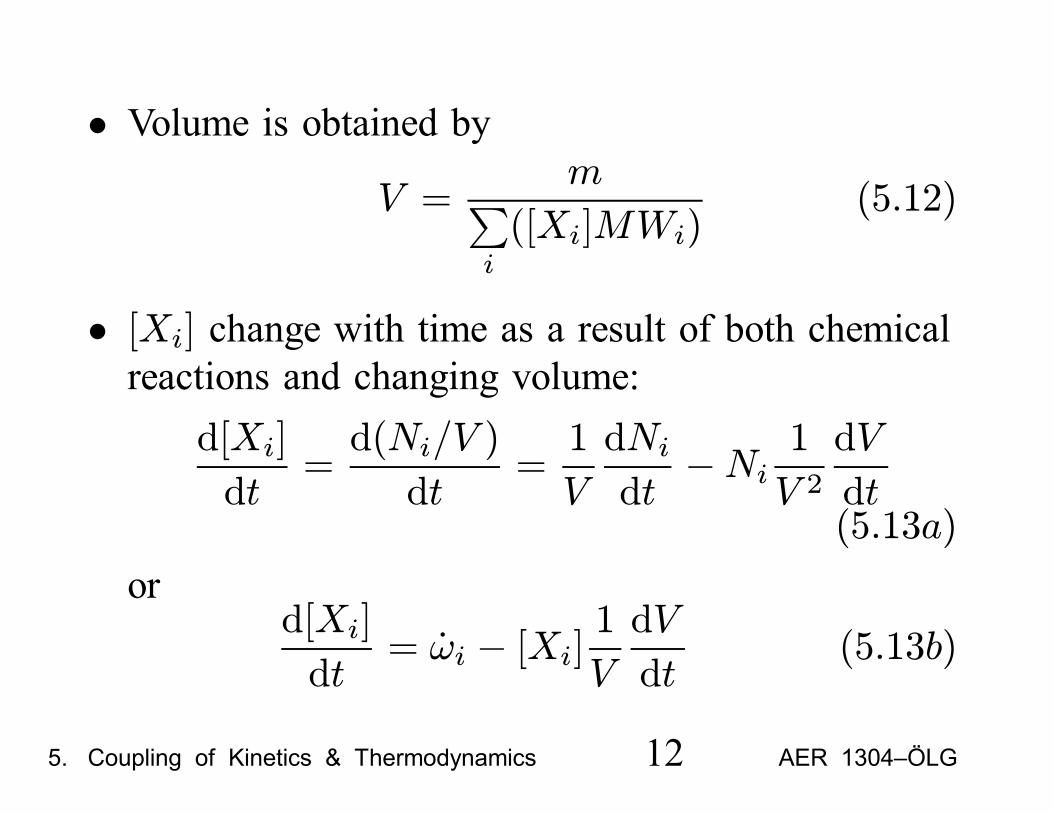
• Volume is obtained byV =

m

i

([Xi]MWi)(5.12)

• [Xi] change with time as a result of both chemicalreactions and changing volume:

d[Xi]

dt=d(Ni/V )

dt=1

V

dNidt−Ni 1

V 2dV

dt(5.13a)

ord[Xi]

dt= ωi − [Xi] 1

V

dV

dt(5.13b)


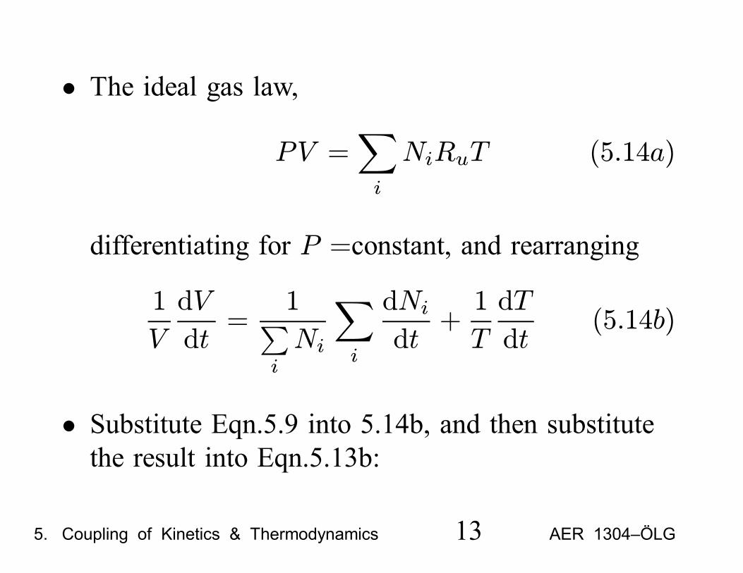
• The ideal gas law,

PV =i

NiRuT (5.14a)

differentiating for P =constant, and rearranging

1

V

dV

dt=

1

i

Ni i

dNidt

+1

T

dT

dt(5.14b)

• Substitute Eqn.5.9 into 5.14b, and then substitutethe result into Eqn.5.13b:


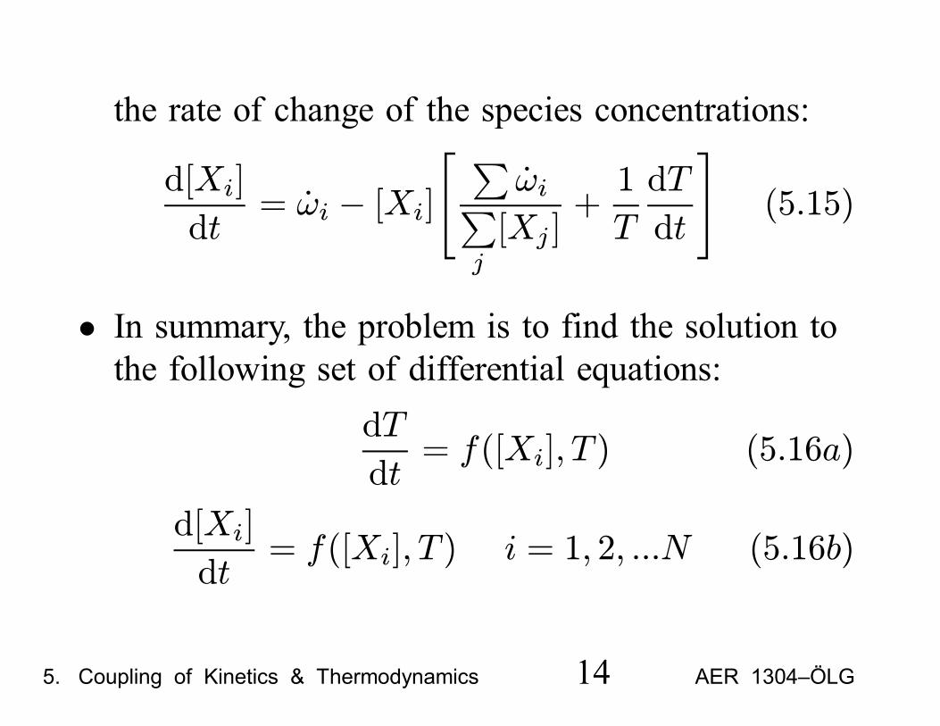
the rate of change of the species concentrations:

d[Xi]

dt= ωi − [Xi] ωi

j

[Xj ]+1

T

dT

dt(5.15)

• In summary, the problem is to find the solution tothe following set of differential equations:

dT

dt= f([Xi], T ) (5.16a)

d[Xi]

dt= f([Xi], T ) i = 1, 2, ...N (5.16b)


subject to following initial conditions:

T (t = 0) = T0 (5.17a)

[Xi](t = 0) = [Xi]0 (5.17b)

• Functional forms of Eqns. 5.17a and 5.17b areobtained from Eqns. 5.10 and 5.15. Eqn.5.11gives enthalpy and Eqn.5.12 gives volume.

• Most of the time there is no analytical solution.Numerical integration can be done using an inte-gration routine capable of handling stiff equations.


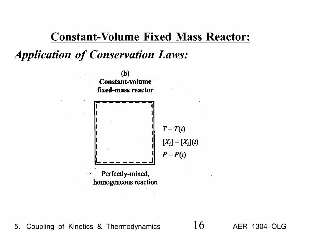
Constant-Volume Fixed Mass Reactor:Application of Conservation Laws:


• Application of energy conservation to the constant-volume fixed mass reactor is similar to constant-pressure case; only exception is W = 0 forV =constant:

du

dt=Q

m(5.18)

• Noting that u now plays the same role as h in ouranalysis for P =constant, expressions equivalentto Eqns.5.5-5.7 can be developed and substitutedin Eqn.5.18. This will give, after rearrangement,


dT

dt=

(Q/V )−i

(uiωi)

i

([Xi]cv,i)(5.19)

Since ui = hi −RuT and cv,i = cp,i −Ru

dT

dt=

(Q/V ) +RuTi

ωi −i

(hiωi)

i

([Xi]cp,i −Ru) (5.20)

• dP/dt is important in V =const. problems.


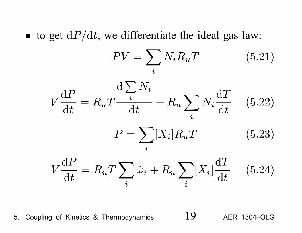
• to get dP/dt, we differentiate the ideal gas law:PV =

i

NiRuT (5.21)

VdP

dt= RuT

di

Ni

dt+Ru

i

NidT

dt(5.22)

P =i

[Xi]RuT (5.23)

VdP

dt= RuT

i

ωi +Rui

[Xi]dT

dt(5.24)


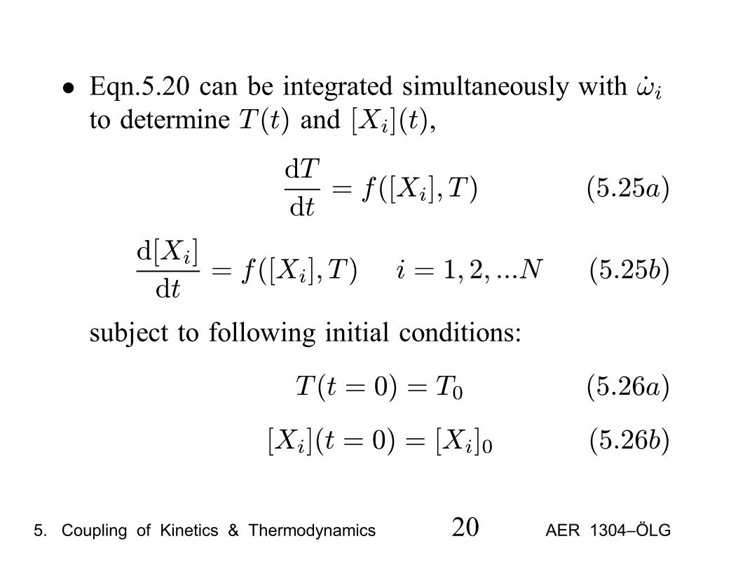
• Eqn.5.20 can be integrated simultaneously with ωito determine T (t) and [Xi](t),

dT

dt= f([Xi], T ) (5.25a)

d[Xi]

dt= f([Xi], T ) i = 1, 2, ...N (5.25b)

subject to following initial conditions:

T (t = 0) = T0 (5.26a)

[Xi](t = 0) = [Xi]0 (5.26b)


Well-Stirred Reactor:• Also called “perfectly-stirred reactor”. Ideal reac-tor with perfect mixing achieved inside the controlvolume.

• Experimentally used for:- flame stability,- pollutant formation, and- obtaining global reaction parameters.

• “Longwell reactor”.• “Zeldovich reactor”.


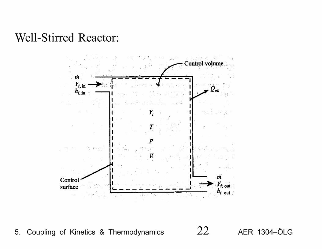
Well-Stirred Reactor:


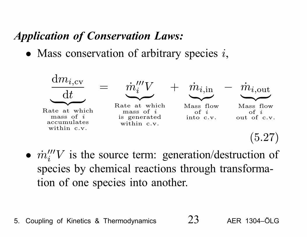
Application of Conservation Laws:• Mass conservation of arbitrary species i,

dmi,cv

dtRate at whichmass of iaccumulateswithin c.v.

= mi V

Rate at whichmass of iis generatedwithin c.v.

+ mi,in

Mass flowof i

into c.v.

− mi,out

Mass flowof i

out of c.v.

(5.27)

• mi V is the source term: generation/destruction ofspecies by chemical reactions through transforma-tion of one species into another.


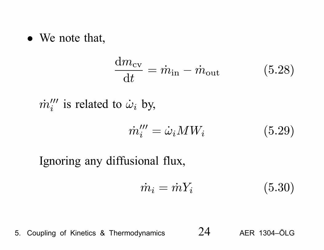
• We note that,dmcv

dt= min − mout (5.28)

mi is related to ωi by,

mi = ωiMWi (5.29)

Ignoring any diffusional flux,

mi = mYi (5.30)


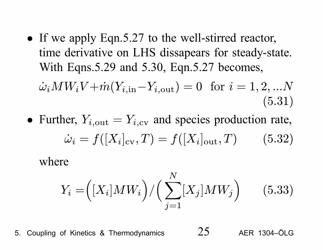
• If we apply Eqn.5.27 to the well-stirred reactor,time derivative on LHS dissapears for steady-state.With Eqns.5.29 and 5.30, Eqn.5.27 becomes,ωiMWiV +m(Yi,in−Yi,out) = 0 for i = 1, 2, ...N

(5.31)

• Further, Yi,out = Yi,cv and species production rate,ωi = f([Xi]cv, T ) = f([Xi]out, T ) (5.32)

where

Yi = [Xi]MWi /N

j=1

[Xj ]MWj (5.33)


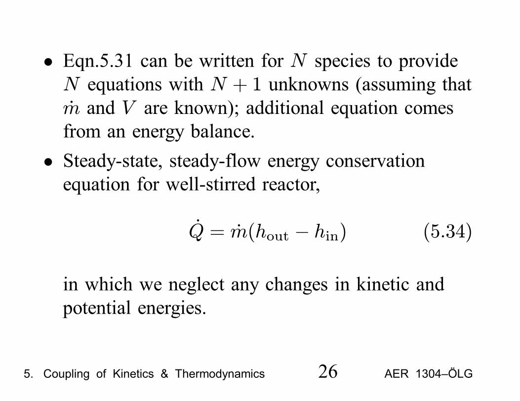
• Eqn.5.31 can be written for N species to provideN equations with N + 1 unknowns (assuming thatm and V are known); additional equation comesfrom an energy balance.

• Steady-state, steady-flow energy conservationequation for well-stirred reactor,

Q = m(hout − hin) (5.34)

in which we neglect any changes in kinetic andpotential energies.


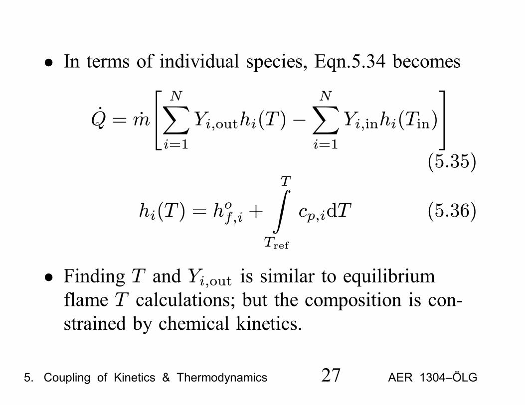
• In terms of individual species, Eqn.5.34 becomes

Q = mN

i=1

Yi,outhi(T )−N

i=1

Yi,inhi(Tin)

(5.35)

hi(T ) = hof,i +

T

Tref

cp,idT (5.36)

• Finding T and Yi,out is similar to equilibriumflame T calculations; but the composition is con-strained by chemical kinetics.


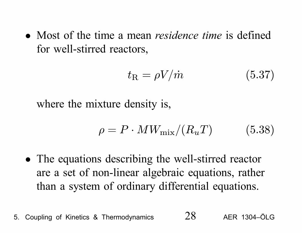
• Most of the time a mean residence time is definedfor well-stirred reactors,

tR = ρV/m (5.37)

where the mixture density is,

ρ = P ·MWmix/(RuT ) (5.38)

• The equations describing the well-stirred reactorare a set of non-linear algebraic equations, ratherthan a system of ordinary differential equations.


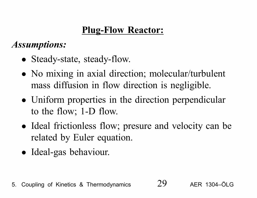
Plug-Flow Reactor:Assumptions:• Steady-state, steady-flow.• No mixing in axial direction; molecular/turbulentmass diffusion in flow direction is negligible.

• Uniform properties in the direction perpendicularto the flow; 1-D flow.

• Ideal frictionless flow; presure and velocity can berelated by Euler equation.

• Ideal-gas behaviour.


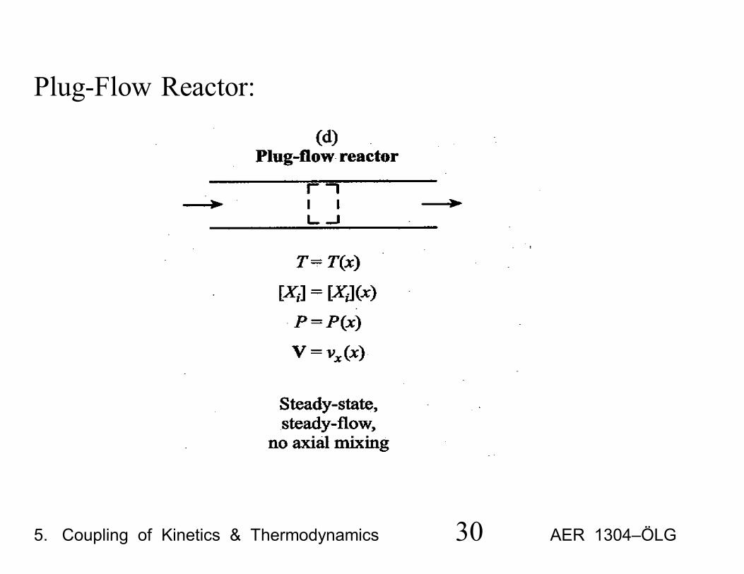
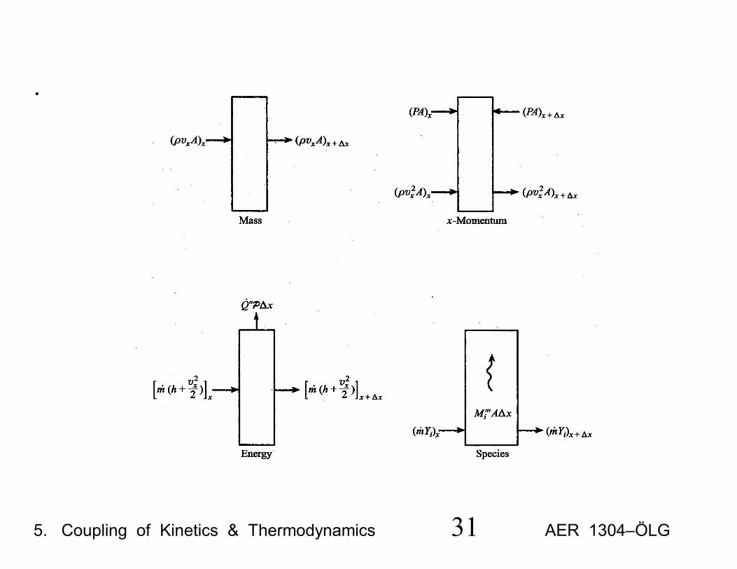
Plug-Flow Reactor:


.


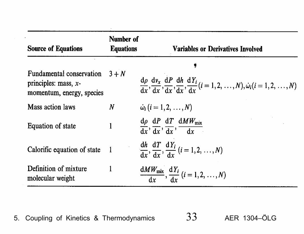
Application of Conservation Laws:• The goal is to develop a system of 1st order ODEswhose solution describes the reactor flow proper-ties as functions of axial distance, x.

• 6 + 2N equations and unkowns/functions.• Number of unknowns can be reduced by N notingthat ωi can be expressed in terms of Yi.

• Known quantities: m, ki, A(x), and Q (x) .• Q (x) may be calculated from a given wall tem-perature distribution.


.


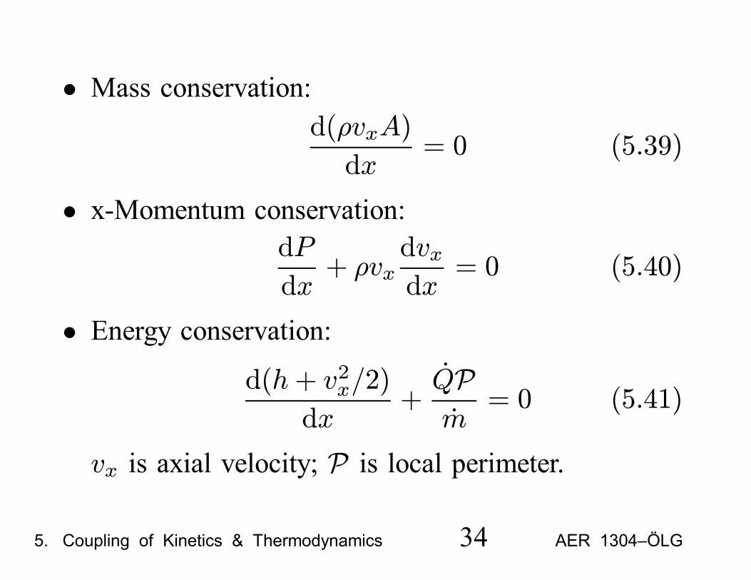
• Mass conservation:d(ρvxA)

dx= 0 (5.39)

• x-Momentum conservation:dP

dx+ ρvx

dvxdx

= 0 (5.40)

• Energy conservation:d(h+ v2x/2)

dx+QPm

= 0 (5.41)

vx is axial velocity; P is local perimeter.


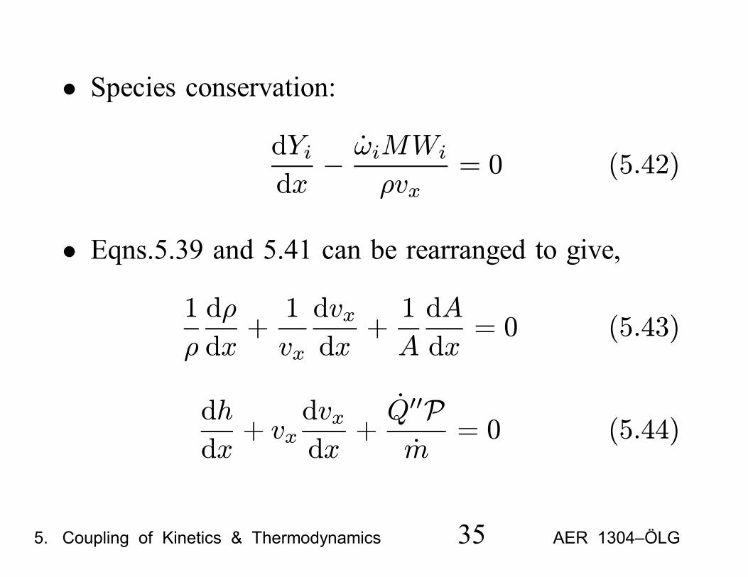
• Species conservation:dYidx− ωiMWi

ρvx= 0 (5.42)

• Eqns.5.39 and 5.41 can be rearranged to give,1

ρ

dρ

dx+1

vx

dvxdx

+1

A

dA

dx= 0 (5.43)

dh

dx+ vx

dvxdx

+Q Pm

= 0 (5.44)


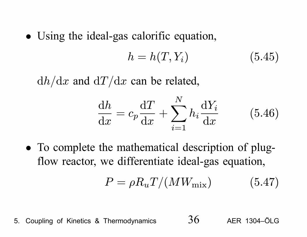
• Using the ideal-gas calorific equation,h = h(T, Yi) (5.45)

dh/dx and dT/dx can be related,

dh

dx= cp

dT

dx+

N

i=1

hidYidx

(5.46)

• To complete the mathematical description of plug-flow reactor, we differentiate ideal-gas equation,

P = ρRuT/(MWmix) (5.47)


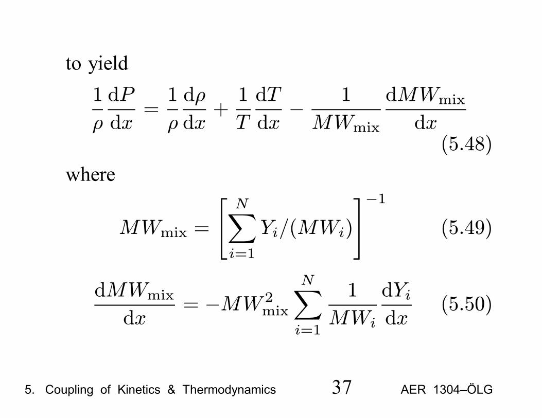
to yield1

ρ

dP

dx=1

ρ

dρ

dx+1

T

dT

dx− 1

MWmix

dMWmix

dx(5.48)

where

MWmix =N

i=1

Yi/(MWi)

−1(5.49)

dMWmix

dx= −MW 2

mix

N

i=1

1

MWi

dYidx

(5.50)


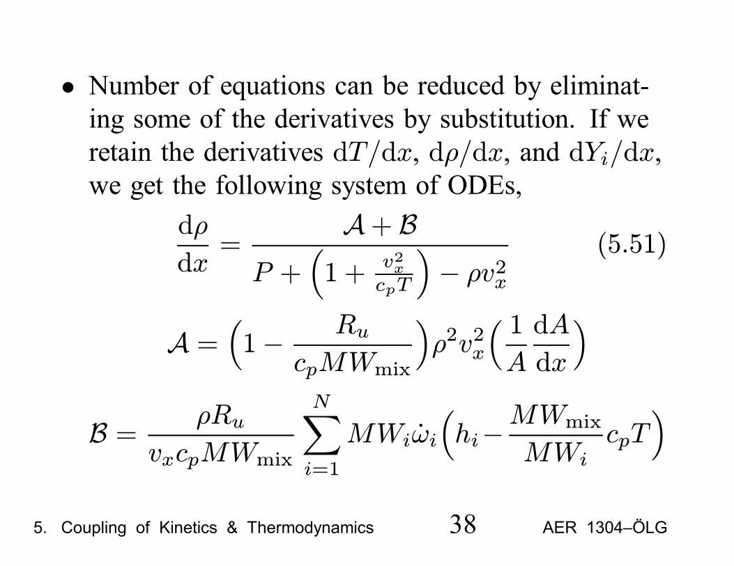
• Number of equations can be reduced by eliminat-ing some of the derivatives by substitution. If weretain the derivatives dT/dx, dρ/dx, and dYi/dx,we get the following system of ODEs,

dρ

dx=

A+ BP + 1 +

v2xcpT

− ρv2x(5.51)

A = 1− RucpMWmix

ρ2v2x1

A

dA

dx

B = ρRuvxcpMWmix

N

i=1

MWiωi hi−MWmix

MWicpT


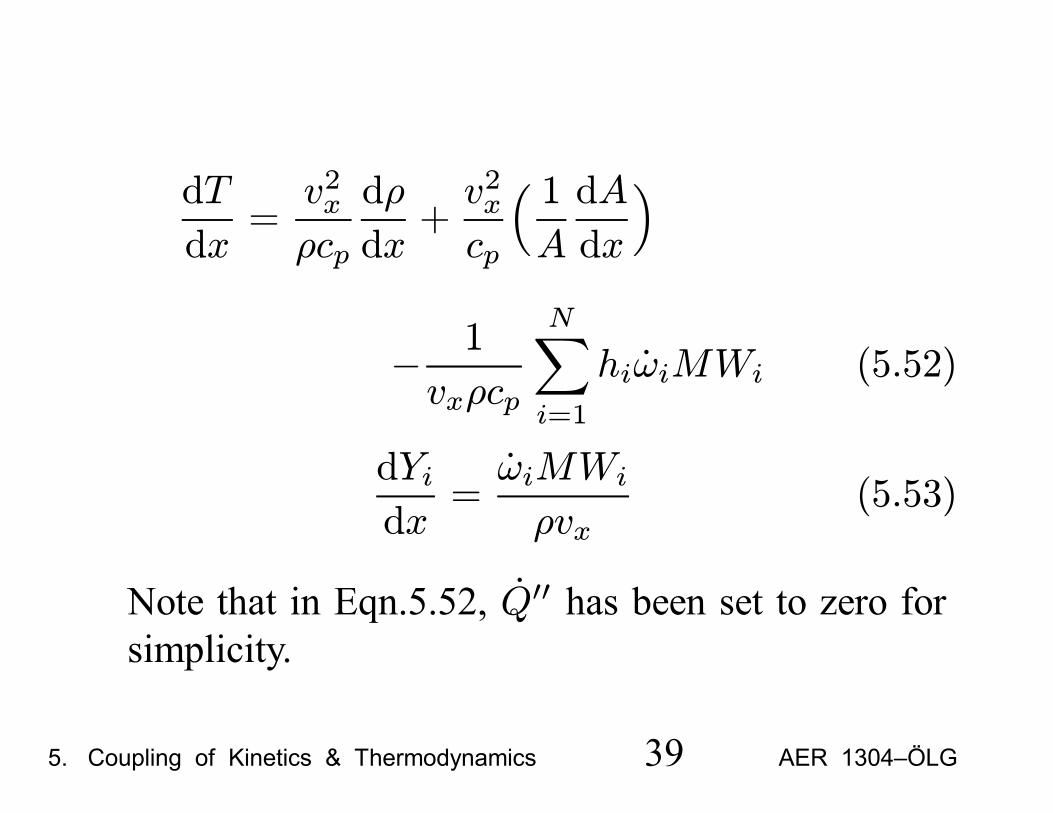
dT

dx=v2xρcp

dρ

dx+v2xcp

1

A

dA

dx

− 1

vxρcp

N

i=1

hiωiMWi (5.52)

dYidx

=ωiMWi

ρvx(5.53)

Note that in Eqn.5.52, Q has been set to zero forsimplicity.


• A residence time can be defined, which adds onemore equation,

dtRdx

=1

vx(5.54)

• Initial conditions to solve Eqns.5.51-5.64 areT (0) = To (5.55a)

ρ(0) = ρo (5, 55b)

Yi(0) = Yio i = 1, 2, .....N (5.55c)

tR(0) = 0. (5.55d)


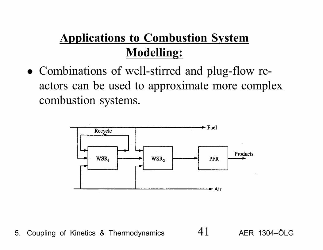
Applications to Combustion SystemModelling:

• Combinations of well-stirred and plug-flow re-actors can be used to approximate more complexcombustion systems.


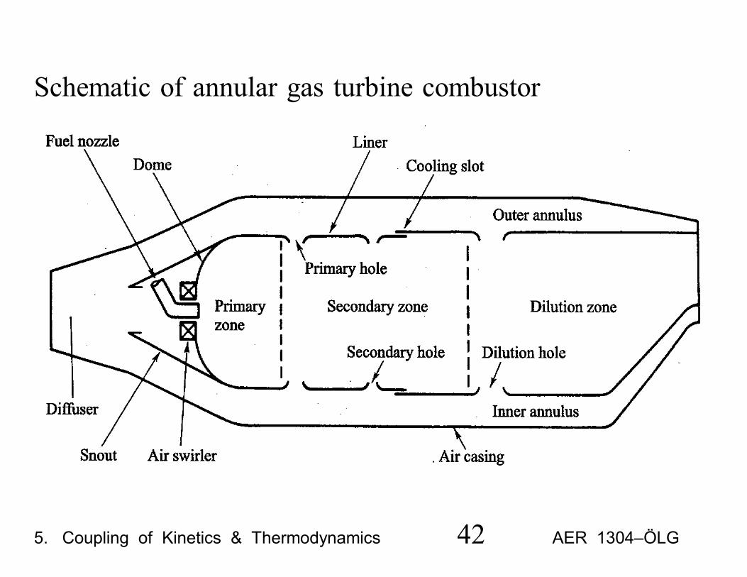
Schematic of annular gas turbine combustor


• Gas turbine combustor is modelled as two well-stirred reactors and a plug-flow reactor.- WSR1: primary zone with recirculation ofcombustion products.

- WSR2: secondary zone.- PFR: dilution zone.

• Reactor modelling approaches are often used ascomplementary tools to more sophisticated finite-element or finite-difference numerical models ofcombustion chambers.


Documents

5. Coupling of Chemical Kinetics & Thermodynamicsarrow.utias.utoronto.ca/~ogulder/ClassNotes5.pdf · • Using definition of enthalpy h ≡u + Pv,and differentiating ... • Also