5 An introduction to Yang-Mills theory

5.1 Introduction

How can we construct successful new scientific theories? If there’s some phenomenon inthe Universe that current theories don’t seem to explain — like dark matter, dark en-ergy, neutrino oscillations or quantum gravity — it’s tempting to throw out our currenttheories, and start over from scratch. Unfortunately, this gives us too much freedomin constructing new theories. Historically, a more successful approach has been to useexisting theories to identify useful overarching principles that can guide the developmentof new theories. So, for example, classical mechanics led to the principle of conserva-tion of energy and the ideas of Hamiltonian mechanics, ideas that played an importantrole in the development of quantum mechanics, even as classical mechanics itself wassuperseded.

Since 1954, one of the most important guiding principles in physics has been thatour description of the world should be based on a special type of classical field theoryknown as a Yang-Mills theory. With the exception of gravitation, all the importanttheories of modern physics are quantized versions of Yang-Mills theories. These includequantum electrodynamics, the electroweak theory of Salam and Weinberg, the standardmodel of particle physics, and the GUTs (grand unified theories) proposed in the 1970sas extensions of the standard model.

The most important of these theories is the standard model of particle physics,which is our current best theory of how matter works. People sometimes describe thestandard model as a Yang-Mills theory with an U(1)×SU(2)×SU(3) gauge symmetry.The purpose of these notes is to explain what this statement means. In particular,I will explain what a (classical) Yang-Mills theory is, and what it means to have agauge symmetry. I won’t explain the standard model itself, since it requires a detaileddiscussion of how to quantize a field theory, which would take us too far afield. However,the treatment here should leave you well prepared to understand the standard modeland related ideas such as GUTs.

The notes assume a fair bit of background, and are aimed at graduate-level (or above)physicists or mathematicians with no prior exposure to the Yang-Mills equations. I as-sume you are comfortable with special relativity and Minkowski space, and with therelativistic formulation of Maxwell’s equations, including concepts such as the Faradaytensor, and the current and potential four-vectors. You should be comfortable with ele-mentary groups such as SU(n), and with the idea of group representations, although wewon’t be using any sophisticated group theory or group representation theory. Finally,you’ll need to be comfortable with calculus on curved surfaces. You won’t need to knowdifferential geometry, although the going will be easier if you have some prior exposureto differential geometry, such as is given in a course on general relativity.

History: The history of Yang-Mills theory is long and twisted. Many of the coreideas were developed independently by physicists and mathematicians, for completelydifferent reasons, and it wasn’t until the 1970s that the links between the two points of

18

view were worked out.In physics, the first example of a Yang-Mills theory was Maxwell’s theory of electro-

magnetism. However, Maxwell and his contemporaries had no idea what a Yang-Millstheory is, and certainly didn’t think of the Maxwell equations in this way! It wasn’tuntil much later that the idea of a gauge symmetry was formulated, and it became un-derstood that Maxwell’s equations satisfy such a symmetry. And it wasn’t until laterstill that Yang-Mills theories were introduced as a large class of theories satisfying gaugesymmetries.

Before the discovery of gauge symmetry and Yang-Mills theory, several people, in-cluding Lorentz, Einstein, and Poincare had studied the symmetries in Maxwell’s equa-tions. They discovered an unexpected symmetry, the Lorentz symmetry, which of courselies at the heart of special relativity. This led other people to investigate whether thereare further symmetries of Maxwell’s equations, and Weyl2 discovered a new symmetryof electromagnetism, now known as gauge symmetry.

Along a different track of development, and a little earlier, Einstein discovered hisgeneral theory of relativity. One of the key ideas that helped Einstein write down thefield equations of general relativity was a symmetry principle, namely, the idea that thefield equations should be the same in every co-ordinate system. In the modern point ofview, this too is an example of a gauge symmetry.

In a famous 1954 paper, Yang and Mills proposed a large class of classical fieldtheories generalizing and inspired by electromagnetism, and satisfying a generalized typeof gauge symmetry. When quantized, these Yang-Mills theories became the mainstay fordevelopments in particle physics in the second half of the twentieth century. As notedabove, examples of quantized Yang-Mills theories include many of our most importantand successful physical theories, including quantum electrodynamics, the electroweaktheory, the standard model of particle physics, and the GUTs (grand unified theories).Crucially, however, although general relativity satisfies a gauge symmetry, it is notknown whether it is possible to cast general relativity as a Yang-Mills theory. This ishighly unfortunate, since we understand how to quantize Yang-Mills theories, but notgeneral gauge theories!

All the successful quantized Yang-Mills theories listed in the last paragraph followthe same general plan. We start from the assumption that the correct theory of the worldis a quantized Lorentz-invariant Yang-Mills theory, and that all that has to be specifiedis the exact nature of the gauge symmetry. This is what the “U(1) × SU(2) × SU(3)”is all about in the description of the gauge symmetry — it is a group which specifiesthe nature of the gauge symmetry. With the gauge symmetry fixed, the classical Yang-Mills theory is completely determined, and by quantizing it one can obtain the standardmodel3.

Once you’ve read the notes, you should understand the basic equations of Yang-Mills2I believe it was Weyl. I haven’t read the original papers, and am relying on hearsay.3Almost. There is one extra ingredient — the Higgs field — that I believe needs to be added in by

hand. But this procedure gives you most of the structure of the standard model.

19

theory. In particular, I’ll explain how you can start with a representation of a group,G, and construct the corresponding Yang-Mills theory. As an example, I’ll explain howMaxwell’s equations can be regarded as a Yang-Mills theory with gauge group U(1). Iwon’t explain the U(1)×SU(2)×SU(3) Yang-Mills theory in any detail, but in principleit is easy to construct using the recipe I will explain.

Now, there is a certain sense in which all this material is pretty easy to explain. Icould just write the Yang-Mills equations out in full detail, and in some sense you’d“understand” Yang-Mills theory. However, merely knowing the equations is not thesame as having a deep understanding of them. In the case of Yang-Mills theory, a deeperunderstanding is obtained if you understand certain geometric ideas behind Yang-Millstheory, and so I’m going to explain much of the geometric context. One reason for doingthis is that the standard model is only one of two great theories of modern physics —the theory of gravitation (general relativity) is the other — and we don’t know how toput the two together. However, both Yang-Mills theories and general relativity can beunderstood using very similar (though not quite the same) geometric ideas, and so itseems worth trying to understand them both from a geometric point of view.

Taking this geometric point of view means we need to work harder than if we justwrite the equations down directly. In particular, I’m going to explain quite a bit ofbackground in differential geometry. The end result is, I hope, a deeper understand-ing of and appreciation for Yang-Mills theory than if we had simply started with theequations alone. Of course, this does not mean that we will obtain a comprehensive un-derstanding of the Yang-Mills equations. Far from it — such an understanding cannotpossibly be obtained by reading a short set of notes on the subject. This should not besurprising, since the Yang-Mills equations generalize Maxwell’s equations, and under-standing Maxwell’s equations even passingly well requires years of work. To develop abetter understanding, you must study them in much greater depth, and in particularunderstand them from multiple points of view, not just the geometric point of view wetake here.

Having expounded on the benefits of geometry, let me note that if I were to rewritethese notes, I would probably not take the geometric viewpoint! While this is a veryuseful and powerful point of view, it is has three significant disadvantages: (1) I don’tthink it is the simplest and most direct way of seeing Yang-Mills theory; (2) it burdensthe beginner with a heavy load of definitions from differential geometry; and (3) thedefinitions can make it more difficult to see the physical forest for all the mathematicaltrees. From an expository point of view, one is forced to compromise between stating thedefinitions as quickly as possible, and a more lengthy exposition that fully motivates thedefinitions. Unfortunately, the definitions of modern differential geometry were arrivedat over a painful process that took approximately 100 years, and understanding theirmotivation in depth is a lengthy task.

Despite all this, I still believe the geometric point of view is well worth studying, andthat the notes may therefore be very useful! But in the future I hope to rewrite themfrom a rather different point of view, perhaps as part of a more extended treatment.

20

What we don’t cover: Before jumping into a description of Yang-Mills theories,let me list a few important topics related to Yang-Mills theories that I’m not going totalk about.

First, although I write down the basic equations of Yang-Mills theory, I won’t bederiving them from a Lagrangian (i.e., least-action) formulation. The ambitious readerfamiliar with least action principles might like to try deriving the Lagrangian formulationas an exercise. However, I decided that a full exposition of these ideas would add toomuch extra length to the article.

Second, everything we do is classical. To get to the standard model or the otherquantum field theories of most interest in modern physics, we need to quantize thetheory. This is, of course, a substantial topic in its own right, and is covered in any texton quantum field theory.

Third, the Yang-Mills theories that we construct are theories with a tremendousamount of symmetry. One of the most famous results in physics is Noether’s theorem,which links continuous symmetries to conserved quantities in the system. We won’t befollowing this link up, even though it cries out to be explored in detail.

Fourth, a critical point about Yang-Mills theories is that they are examples of renor-malizable theories. Without explaining what renormalizability is all about, I will justsay that it it is a critical property for a field theory to have if it is to be useful forcomputing finite quantities4.

Acknowledgements: I learnt about gauge theory and Yang-Mills theory fromthe beautiful book “Gauge Fields, Knots and Gravity”, by John Baez and Javier P.Muniain [1].

5.2 Overview

The Yang-Mills equations are two easily-stated equations:

dDF = 0 (1)∗dD ∗ F = J. (2)

Of course, while they may be easy to write down, that doesn’t mean it’s easy to under-stand what all those symbols means! In this section we develop a conceptual roadmap tounderstanding the Yang-Mills equations. We’ll give a rough description of each elementin the Yang-Mills equations, and hopefully convey something of their overall flavour.You shouldn’t expect to completely understand everything in this section on a firstread. Rather, the purpose is to begin forming a bird’s-eye view that can assist in keep-ing oriented as we move through our detailed later discussions of each of the individualelements.

An unseen but important element of the Yang-Mills equations is the manifold onwhich all the action take place — this is where our physical objects live. In the case

4I believe that it was for providing evidence that Yang-Mills theories are renormalizable that wonGerardus ’t Hooft and Martin Veltman the 2003 Nobel Prize for Physics. However, I haven’t read upon the details of this, and so can’t be sure.

21

of both electromagnetism and the standard model, that manifold is just the Minkowskispace of special relativity. We’ll explain the equations on a general manifold, since itentails little additional complexity, but if you prefer you can always imagine that we areworking on Minkowski space.

The connection, D: The fundamental physical object in the Yang-Mills equationsis the connection, which is denoted D. This shows up only surreptitiously in the equa-tions, as a subscript, albeit twice, but the connection actually determines nearly all theother quantities in the equations, including dD, F , and all the starred quantities, andonly excluding the current, J , which describes the distribution and velocity of chargesin the theory. Thus, if the current is regarded as given, then the Yang-Mills equationsare really just a set of equations that constrain the connection, D.

Mathematically, the connection tells us how to move stuff around from point topoint on the manifold — it’s a means for achieving so-called “parallel transport” onthe manifold. If you’ve taken a course in general relativity you’ve met an example of aconnection; the notion we’ll be talking about is essentially the same idea, although weneed it in a more general form than how it’s used in general relativity.

Physically, the connection is the fundamental physical field of the theory. Togetherwith the current, J , the connection completely determines all the physical propertiesof the system. In the case where the Yang-Mills theory is Maxwell’s equations, theconnection is essentially just the electromagnetic vector potential.

It should be apparent to you from this description that the mathematical and phys-ical meanings of the connection are very different! So far as I am aware, there is nogood reason known why we should expect these two notions to coincide. Stated anotherway, the physicists don’t know why their notion of a field should also play a role in thedescription of parallel transport, and the mathematicians don’t know why the objectthey use to describe parallel transport should have any physical significance as a field.Indeed, the co-inventor of Yang-Mills theories, Yang, has recalled that he didn’t evenlearn what a connection is until 1975, twenty-one years after he and Mills proposedYang-Mills theory. From his point of view, he was simply writing down a physical fieldto generalize the vector potential of electromagnetism.

The curvature, F : We’ve seen that the connection plays a role analogous to thevector potential in Maxwell’s equations. Of course, we don’t ordinarily write Maxwell’sequations directly in terms of the vector potential, but rather work in terms of derivedquantities, namely the electric and magnetic fields, or, if we are a bit more sophisticated,in terms of the Faraday tensor.

In Yang-Mills theory, the Faraday tensor is generalized to the curvature, F . Math-ematically, the curvature is derived from the connection essentially by taking commu-tators of certain differential operators related to the connection. Physically, as alreadystated, you should think of the curvature as generalizing the Faraday tensor in electro-magnetism; it (rather than D) is what most directly acts on physical particles.

If you’ve met the concept of curvature previously, then you probably know thatthe way we ordinarily conceive of Minkowski space it is a flat (i.e., uncurved) space.

22

However, the idea of Yang-Mills theory is to throw out the ordinary concept of flatMinkowski space. What the connection (e.g., the vector potential) does is to introducea “twist” into Minkowski space. The curvature F then measures the extent to whichthis twist causes a deviation from the ordinary flat geometry of Minkowski space.

The exterior covariant derivative, dD: The operation dD is known as the exteriorcovariant derivative. Very roughly speaking, the quantity dDX is a measure of how fastX is changing as it is moved around in various directions on the manifold. The Yang-Mills equations thus tell us that, in a certain sense, F is not changing as we move aroundthe manifold, while the way ∗F changes is determined by the current, J .

Now, this is pretty clearly nonsense! After all, in electromagnetism the Faradaytensor F certainly can change. However, recall above that I said that the connectioncauses a “twist” in Minkowski space. In fact, in some sense the Yang-Mills equationdDF = 0 is telling us that, with respect to this twist, F is not changing5.

The Hodge ∗-operation: The final element in the Yang-Mills equations is theHodge ∗-operation. This is applied twice in the second Yang-Mills equation, first to F toobtain ∗F , and then to dD ∗F to obtain ∗dD ∗F . To understand the role of the Hodge-∗,recall that in the conventional Maxwell equations it is possible to interchange the E andB fields, provided one ignores the source ρ and current j terms, and makes suitable signchanges and rescaling. The Hodge ∗-operation is a generalization, interchanging certaintemporal degrees of freedom (generalizing the E field) and certain spatial degrees offreedom (generalizing the B field).

What about the Lorentz force law? As we have seen, the Yang-Mills equationsgeneralize the Maxwell equations for electromagnetism. However, the Maxwell equationsare not, on their own, a complete set of equations for a physical theory. They must besupplemented by an additional law, the Lorentz force law, that tells us how chargedparticles accelerate in an electromagnetic field. The Lorentz force law for a particle ofmass m and charge q is

muj = qF jku

k, (3)

where uj are the components of the velocity four-vector, uj indicates the derivative withrespect to proper time, and F j

k are the components of the Faraday tensor. This equationcannot be deduced from the Maxwell equations. This can be seen since the mass playsa critical role in the Lorentz force law, while it is completely absent from the Maxwellequations.

While the Maxwell equations don’t specify a complete physical theory, the Maxwell-Lorentz equations do. In particular, if we are given an initial configuration of charges,currents and fields, then the Maxwell-Lorentz equations tell us the time rate of changeof all quantities, and so can in principle be integrated forward in time to tell us the

5Actually, it’s a bit more complicated than that. Consider the equation ∇ · B = 0 from Maxwell’sequations. This doesn’t tell us that B is not changing, just that the total flux of B from a volume isalways zero. The equation dDF = 0 has more of this nature.

23

configuration at later times6.Can we generalize the Lorentz force law so that it applies also to Yang-Mills theories?

Unfortunately, although such a generalization is certainly known, it is not (yet) known byme! The obvious generalization is to simply replace the Faraday tensor by the curvature.This certainly does not work, as we shall see later that the curvature acts on the wrongspace. Finding a suitable generalization could certainly be done by starting with one ofthe standard Lagrangians describing the interaction of a Yang-Mills field with matter(e.g., such as arise in the standard model), but I haven’t actually gone through andworked out the details.

Incidentally, I said above that particles most directly feel curvature, rather thanthe connection. It should be clear from the discussion in the last paragraph that Iwas blowing hot air with that statement (excusably, I hope). Without a generalizationof the Lorentz force law to arbitrary Yang-Mills theories, we can’t say this for sure.Nonetheless, I hope you will agree that it seems highly likely.

A warning about Yang-Mills theories: The Maxwell-Lorentz equations havesome significant problems as theories of physics, and it seems reasonable to supposethat similar problems occur in most other Yang-Mills theories. Particularly problematicin electromagnetism is what happens when you look up close at a charge. Consider, forexample, an electron. How should we model the electron in the Maxwell-Lorentz theoryof electromagnetism?

One way is to imagine that the electron is a simple point charge. Unfortunately,the Coulomb law tells us that there must be a singularity in the field at the point theelectron sits at. The field isn’t defined at that point, and the Lorentz force law cannotbe applied; the theory doesn’t tell us which way the electron should move! Althoughvarious ad hoc fixes to this problem can be applied, and in practice are, there does notseem to be a conceptually clean and simple way of modifying the theory so this problemis avoided.

A second posssibility is to imagine that the electron is a smeared out ball of charge.This solves the problem with the singularity in the field, but raises the problem of whythe electron doesn’t fly apart due to the tremendous internal repulsive forces? Onemight try to solve this problem by positing the existing of countervailing forces thathold the electron together, but I do not know of a successful and simple theory in thisvein.

All this should make you uneasy. After all, the standard model — one of the greatestachievements of science — is a quantized Yang-Mills theory. We’ve obtained the stan-dard model by starting with a theory with serious conceptual problems, then applyingan ad hoc quantization procedure to that theory. Lo, by some process of alchemy abeautiful theory is revealed, explaining most of what we see in the world. Now, thisprocedure of quantizing Yang-Mills theories has been so fantastically successful that it

6I am, as physicists often do, ignoring all questions of whether or not singularities might arise thatmake it impossible to continue the process of integration, merely assuming that these equations aresufficiently nice that this will never be the case.

24

deserves to be taken very seriously as a means of finding new theories. But that certainlydoesn’t mean that you should be comfortable with it!

Exercise 5.1: One possible idea for understanding the structure of the electron is tosuppose that it is gravitation which is holding the electron together against theinternal forces of repulsion. Show that this doesn’t work, that gravitation is fartoo weak to be the force responsible for holding the electron together internally.

Why have Yang-Mills theories been so successful? To answer this question,it is necessary to think about the more fundamental question of how one should studydynamics. Naively, it is tempting to study dynamics directly, trying to directly observethe effect of the forces that hold stuff together. This approach has, of course, beenvery successful, and has a long tradition going back to phenomena such as Newton’sdiscovery of the inverse square law (which has its roots in the work of Brahe, Kepler,and Galileo), and is still used even today.

The twentieth century brought another idea for studying forces to the fore. This isthe idea that one doesn’t need to study them directly, but instead can study symmetriesof the theory, and that if there is enough symmetry those symmetries effectively dictatethe interaction.

In simple forms, this is, of course, an old idea — we know that if two particles arethe “same” then quantities such as the Hamiltonian or Lagrangian should be invariantunder interchange of the two particles, and this constrains the form of those quantities.

However, this idea can be taken much further. In particular, if we choose a sufficientlylarge class of symmetries, then this greatly constrains the class of physical theories thatare allowed. In some cases, this constraint is so great that symmetry plus a few othersimple physical principles becomes sufficient to uniquely pick out our theory. This was,for example, the case for Einstein’s general theory of relativity.

How do the Yang-Mills equations fit into this picture? Essentially, they can be viewedas a machine which takes as input a heavy symmetry constraint — the constraint ofinvariane with respect to some gauge symmetry that we specify — and produces asoutput a classical field theory satisfying that constraint. Furthermore, that classicalfield theory turns out to have many other desirable features, such as renormalizability.Thus, the Yang-Mills approach offers an excellent sandbox for constructing interestingtheories. It is broad and rich, in that we can specify many different types of symmetrygroup, and thus describe many different types of physics. At the same time, Yang-Millstheories have properties such as renormalizability which make them suitable for use ina quantized description.

5.3 Background on differential geometry

We are taking a geometric approach to the Yang-Mills equations. This poses an expos-itory challenge, for I do not wish to assume you are familiar with differential geometry.Unfortunately, understanding even elementary differential geometry requires mastering

25

a large body of definitions. In some sense, the most efficient way of mastering thismaterial is simply to proceed through 40 or 50 pages of definitions, covering topologicalspaces, smooth manifolds, tangent vectors and so on, with occasional lemmas and the-orems mostly of technical interest. Most books on differential geometry proceed in thisfashion before getting to the truly interesting theorems of differential geometry.

In my opinion this approach is not suitable for us for two reasons.First, on general grounds, I don’t believe this long line of definitions is a good

approach. Definitions are not made in a vacuum, they have a historical context andreason, often being made in response to some mathematical or scientific problem, orbecause someone sees a clever way of generalizing earlier results. They are almostalways inextricably linked to the reasoning used in theorems; often alternate definitionsare tried and dropped when it is realized that they don’t have quite the right propertiesto make the line of reasoning in the proof of some theorem or another work. In the case ofdifferential geometry, it took approximately 100 years for the definitions of “elementary”differential geometry to take their modern form, spanning from the mid 19’th centuryto the mid 20’th century. In the standard expository approach to differential geometrywe see the endpoint of this, but only barely glimpse the underling motivations, all thealternate definitions, now discarded, or the clever way in which some definition is tailoredto a theorem proved one hundred pages later.

Second, our object here is not to become experts in differential geometry. Rather,it is to understand the basic ideas of Yang-Mills theory, and the differential geometryis simply a means to that end. Going through all the detailed definitions of differentialgeometry leaves us in danger of losing sight of our principal purpose.

In view of this, I’m going to cheat a little. Rather than give fully rigorous definitionsfor concepts like manifolds, tangent spaces and so on, in this section I introduce therequired background informally, stating the main ideas, and giving some examples, andfeeling free to ignore issues like smoothness and so on7. This background should besufficient to build up a detailed understanding of objects such as the connection andcurvature, which are central to Yang-Mills theory.

Despite this approach, we still have a sizeable body of definitions to cover, and thereare a few points where I’ll need to gloss over some details — I’ll warn you when I dothis. Nonetheless, I hope this informal approach will let you more quickly appreciatethe Yang-Mills equations, and give you a good feeling for the geometric context in whichthey arise.

Manifolds: The arena for Yang-Mills theory is a general (smooth) manifold, whichwe shall denote generically by M . Manifolds are generalizations of the familiar spaceRn. They can be thought of as smooth surfaces that look locally like Rn, but whichmay have quite a different global structure. For example, the surface of the ordinarysphere looks locally like R2 — this is why people used to think the world is flat — but

7Contrary to what physicists are sometimes taught as undergraduates, these issues are important.But they are subsidiary to our main goal here, which is to understand the broad sweep of Yang-Millstheory, and so we’ll ignore them.

26

of course is really quite different from R2.Now, all our examples of Yang-Mills theory — and all the appplications of Yang-

Mills of most importance in modern physics — are for the case when the manifold M isMinkowski space, which should already be familiar to you from special relativity. Thus,if you simply replace the term “manifold” in all that follows by “Minkowski space”, youshould be able to follow what is going on.

However, to understand the motivation for some of the definitions we make it isuseful to have a second example manifold in mind. An excellent choice is to choose Mto be the surface S2 of a sphere in three dimensions. (Be warned: although I said “inthree dimensions”, of course the surface of the sphere is a two-dimensional manifold,because it looks locally like R2. This is why it is denoted S2.) If you keep both theexample of Minkowski space and S2 in mind as we discuss manifolds, you should be wellplace to understand all the further definitions that we make.

Local co-ordinate systems: Perhaps the most important concept for us in dis-cussing manifolds is the idea of local co-ordinates. Local co-ordinates are, as their nameindicates, a means of describing location in some small region of a manifold. For exam-ple, on a two-dimensional manifold such as S2, around any point x on the sphere we canfind a small surrounding neighbourhood N which can be given local co-ordinates — amap between points in N and co-ordinates (x1, x2) in R2. These co-ordinates uniquelyidentify points in the neighbourhood N . Such local co-ordinate systems are a greatconvenience for making definitions, and for doing calculations, and we shall often findit convenient to introduce a local co-ordinate system.

Incidentally, local co-ordinate representations sometimes get a bad rap in the lit-erature. Some authors go to extremes in attempting to perform calculations withoutthe use of local co-ordinates, sometimes adopting an evangelical tone in advocating thisapproach. This, in my opinion, makes as much sense as insisting that you navigatearound a city without using street numbers: “make a right after the corner store, thena left at the burnt-out tree stump, three blocks up, right again, . . .”. Co-ordinates aresimply another tool — use them if you think they’ll be helpful.

Scalar fields: We’re going to consider many different types of fields on the manifold.As you can no doubt guess, a field simply associates to each point on the manifoldanother object — maybe a number, maybe a vector, or perhaps some other types ofquantity — often intended to represent some physical quantity. So, for example, atemperature field defined on the manifold R3 might be used to model temperature inthe atmosphere. The simplest type of field is a scalar field, which assigns to each pointx on the manifold a number s(x). We’ll find it useful to consider both real and complexscalar fields.

Tangent vectors: One of the most common types of field is a tangent vector field,which assigns to each point x on a manfiold a vector v(x) which is tangent to themanifold. Such tangent vectors can be used to represent a direction of travel on themanifold; a natural physical example of a tangent vector field is the velocity field insidea fluid.

27

Unfortunately, rigorously defining and studying the elementary properties of tangentvectors on a general manifold requires a fair bit of tedious work.

Fortunately, our intuition about tangent vectors is already excellent; the rigorousapproach mostly reveals facts already well known to your intuition. For our purposes,it will therefore suffice to think of the example of S2. In particular, we all know what itmeans for a vector to be tangent to S2 at some point x on S2.

Tangent vectors are easily given co-ordinate representations. If (x1, x2) are local co-ordinates on the manifold defined in a neighbourhood of x, then we see that there arenatural associated tangent vectors e1 and e2, representing motion, respectively, in thedirection of increasing x1 at unit speed, and increasing x2, again at unit speed. A generaltangent vector v at the point x can be written as a linear combination v = v1e1 + v2e2,with the direction and speed of motion obvious. We refer to v1 and v2 as the co-ordinatesfor v with respect to the local co-ordinates (x1, x2). It is often convenient to abbreviatethe local co-ordinates to just xj , and the corresponding co-ordinates for the tangentvector to vj .

The space of all vectors tangent to a given point x ∈M is obviously a vector space,and we denote it by TxM . If M is an n-dimensional manifold, then the tangent spaceTxM also has n dimensions for all points x. So, for example, the tangent spaces TxS

2

to the sphere are all two-dimensional; we can think of TxS2 as the plane tangent to S2

at the point x.With these concepts in mind, it is now easy to define a vector field on a manifold

M as a function assigning to each point x on the manifold a vector v(x) in the tangentspace TxM .

As we have defined them, vector and scalar fields are defined everywhere on the man-ifold. In fact, quite often when dealing with local co-ordinates we will find it convenientto consider a field (vector, scalar, or any other type of field) as being defined just on theneighbourhood in which the co-ordinates are defined.

The commutator of vector fields: Suppose v is a tangent vector at a pointx on a manifold M . Suppose vj are the components of v with respect to some localco-ordinate system xj . It is possible to associate with v a differential operator via thecorrespondence

v ⇔ vj ∂

xj, (4)

where we use the Einstein summation convention. The differential operator on the rightacts on functions defined in the neighbourhood of x in the obvious way, so we have

v(f) = vj ∂f

∂xj. (5)

Why make this correspondence between vectors and differential operators? Unfor-tunately, answering that question fully would take me too far afield, and so I will askyou merely to accept that the correspondence is useful. The main consequence for us

28

is that it allows us to define a sensible notion of a commutator between vector fields vand w. In particular, we can define

[v, w](f) ≡ v(w(f))− w(v(f)). (6)

It is clear that this defines a differential operator [v, w] acting on functions. A priorione might think that this differential operator contained both first- and second-orderderivatives, but in fact some elementary algebra shows that the second-order terms allcancel, leavng just first-order derivatives. Thus, using the correspondence of Eq. (4) inthe other direction we may regard [v, w] as also defining a vector field. A calculationshows that this vector field has components:

[v, w]k = vj ∂wk

∂xj− wj ∂v

k

∂xj. (7)

Exercise 5.2: Verify the co-ordinate representation of Eq. (7).

The co-ordinate vector fields: Suppose we have co-ordinates xj defined on someneighbourhood on the manifold. As we noted above, at any point x in the neighbour-hood, there is a tangent vector ej ∈ TxM pointing in the xj direction on the manifold,and denoting travel at unit speed. It will be convenient to introduce a new notation,∂j ≡ ej , for this tangent vector, motivated by the correspondence with the differentialoperator, ∂/∂xj ; indeed, we shall also use ∂j as shorthand for ∂/∂xj . Note that we canexpand any vector field at any point x in the neighbourhood as v = vj∂j , where thevj are coefficients that depend on x, and we make use of the Einstein summation con-vention. As a result, we call these vector fields a co-ordinate basis or co-ordinate vectorfields for the neighbourhood. For later use it is useful to note that the co-ordinate basiscommutes:

[∂j , ∂k] = 0. (8)

This follows immediately from the representation of Eq. (7).

Exercise 5.3: Suppose xj and xj are two different co-ordinate systems, both definedin neighbourhoods of a point x. Let v be a vector in the tangent space TxM .Convince yourself that the components vj and vj corresponding to the co-ordinatebases ∂j and ∂j are related by

vk =∂xk

∂xjvj . (9)

A useful shorthand notation for this transformation law is

vk = (∂j xk)vj . (10)

29

The inverse transform is clearly

vk =∂xk

∂xjvj = (∂jx

k)vk, (11)

where ∂j ≡ ∂/∂xj . Note that since we haven’t rigorously defined tangent vectors,it’s not possible to provide a rigorous proof of these equations. Nonetheless, youshould be able to convince yourself pretty thoroughly that they are true. Twoapproaches you might take are: (1) to look at examples of different co-ordinatesystems near a point on the sphere; and (2) to start from the point of view inwhich tangent vectors are identified with differential operators.

Cotangent space: To each tangent space TxM we associate a cotangent space,which we denote T ∗

xM . This is the vector space dual to TxM , and consists of linearmaps from TxM into R. Just as TxM has as a basis the vectors ∂j , the cotangent spacehas as a basis dual vectors dxj whose action is defined by

dxj(∂k) ≡ δjk. (12)

Upon first sight, the notation dxj may seem mysterious. It is tempting to think that itmust be associated to calculus in some way, and perhaps represents an infinitesimal. Infact, from the right point of view, there is a close connection to the calculus notions.We’ll begin developing this point of view in Section 5.5, but we won’t develop it to itsfullest conclusion. For our purposes it’s best to think of dxj as simply being a vector inthe space T ∗

xM , and to regard the use of the infinitesimal notation as a coincidence tobe ignored.

One-forms: We saw earlier that a vector field is a function that associates to eachpoint x on the manifold a point v(x) in the tangent space TxM . The analogous notionfor the cotangent space is that of a one-form. By definition, a one-form is a map ω whichtakes points x on the manifold M to an element ω(x) of the corresponding cotangentspace, T ∗

xM .So far, we’ve defined three types of field — scalar fields, vector fields, and one-forms.

This may seem a lot, but Yang-Mills theory requires two further generalizations of thefield concept, known respectively as p-forms (unsurprisngly, they generalize one-forms),and vector bundles. We’ll explain p-forms now, and vector bundles later, in Section 5.7.In Section 5.10 we’ll define a notion of a vector bundle-valued p-form that generalizesand combines both p-forms and vector bundles; it is these vector bundle-valued p-formsthat are the natural objects in Yang-Mills theory.

The wedge product: To explain p-forms, we need to turn away from the contextof differential geometry, to vector spaces. Suppose v1, v2 ∈ V are two elements of avector space V . We define the wedge product of v1 and v2 by

v1 ∧ v2 ≡v1 ⊗ v2 − v2 ⊗ v1

2. (13)

30

We can extend this definition to more vectors, e.g., v1, . . . , vp ∈ V , by

v1 ∧ v2 ∧ . . . ∧ vp ≡∑

π sgn(π)vπ(1) ⊗ vπ(2) ⊗ . . . vπ(p)

p!, (14)

where the sum is over all permutations π of 1, . . . , p, and sgn(π) is +1 if π is an evenpermutation, and −1 if π is an odd permutation. Notice that with this definition, wehave v1 ∧ v2 = −v2 ∧ v1. If we have more vectors, then swapping any two in the wedgeproduct similarly produces a minus sign.

The p’th exterior product of V is the vector space Λp(V ) spanned by vectors of theform v1∧ . . .∧vp. By convention, we choose Λ0(V ) = R, a one-dimensional vector space.

Exercise 5.4: Show that if any two vectors vj and vk in a wedge product v1 ∧ . . .∧ vp

are the same, then the wedge product vanishes.

Exercise 5.5: Show that Λp(V ) = 0 if p ≥ dim(V ).

Exercise 5.6: When 0 ≤ p ≤ dim(V ), show that the dimension of Λp(V ) is(dim(V )

p

).

p-forms: We are now in position to define p-forms, generalizing our earlier definitionof one-forms. To do so, we have to return to differential geometry, and the context ofa manifold, M . A p-form is just a map ω which takes each point x on the manifoldto an element of Λp(T ∗

xM). In the case when p = 1 this reduces to the definition ofa one-form given above, since Λ1(T ∗

xM) = T ∗xM . A 0-form is just a scalar field, since

Λ0(T ∗xM) = R, by convention.

Recall that we had a basis dxj of cotangent vectors for the cotangent space T ∗xM .

Thus, a one-form will look locally something like:

ω = ωjdxj , (15)

where we call the ωj a local co-ordinate representation for the one-form. Similarly, atwo-form can always be expanded in local co-ordinates like

ω = ωjkdxj ∧ dxk. (16)

We denote the set of all p-forms on a manifold M by Ωp(M).

Exercise 5.7: Show that the coefficients ωjk in Eq. (16) can always be chosen so as tobe antisymmetric, i.e., ωjk = −ωkj . Furthermore, prove that this choise is unique.

31

5.4 The difficulty of doing calculus on manifolds

In applications of differential geometry to physics (like Yang-Mills theory) a typicalsetup is that the underlying manifold represents all of spacetime, and that fields onthat manifold are used to describe physical quantities. The equations of physics thendescribe how the time variation of those physical quantities is related to their spatialvariation.

To describe all of this in a precise mathematical fashion, obviously we need a wayof doing calculus on manifolds. Unfortunately, it turns out to be not obvious how todo calculus on manifolds. To see why this is, let’s get some idea of the problems thatarise in trying to define the derivative of a vector field. In particular, suppose v(x) is avector field, and we want to compute its derivative — its rate of change — as we movein some direction y away from the point x (so y ∈ TxM) on the manifold. The naturalguess to make is that the derivative should be the ∆ → 0 limit of the expression

v(x+ ∆y)− v(x)∆

. (17)

The first difficulty in understanding this expression is to understand what x+∆y means.Fortunately, with a little work it turns out that this difficulty can be resolved by workingin a local co-ordinate representation for x and y. Much more serious is the fact thatthe vector v(x + ∆y) lives in the tangent space Tx+∆y, while the vector v(x) lives in acompletely different tangent space TxM , and we have no a priori way of making senseof the difference of these two vectors.

Now, you might object, both vector spaces have the same dimension, surely weshould be able to identify them? Well, okay, but how exactly should we do that? Vectorspaces don’t just come with labels automatically attached that let us identify them withone another. In fact, with a little bit of work we can specify a labelling scheme that letsus identify one tangent space with another, but it turns out to require some care andsubtlety. This is the idea behind the definition of the connection or covariant derivative,which we’ll study in Section 5.6.

Another way of seeing the difficulty is to examine the example of the surface ofthe sphere, S2. Different points on the sphere have different tangent spaces, and it isclear that taking the difference between tangent vectors in different tangent spaces mayend up resulting in a vector that belongs to neither tangent space. Now, you mightobject that at least we get a vector this way. But it should bother you that we’ve takenthe derivative of a two-dimensional vector field, and ended up with a three-dimensionalvector! What’s worse, it turns out that the surface of the sphere, S2, can actuallybe embedded in higher dimensional spaces in multiple ways, and so we don’t get anunambiguous definition even in this way.

Problem for the author 5.1: While I’ve poured scorn on this method of takingderivatives by embedding in a higher-dimensional space, it may be worth investi-gating in more detail. In particular, it is known that any n-dimensional manifold

32

can be embedded in R2n. Might it be possible to construct some canonical em-bedding which allows us to define the derivative in an unambiguous way? Whatproperties might this derivative have?

Because of these difficulties, defining a sensible notion of derivative is a challengefor elementary differential geometry. It turns out that there are two approaches togeneralizing the derivative that have been found to be especially useful — the exteriorderivative, which is defined in the next section, and the covariant derivative, also knownas the connection, which is defined in Section 5.6. In Section 5.10 we’ll define the exteriorcovariant derivative, which combines both these operations.

Why are two notions of derivative needed? I must admit, I don’t understand theanswer to this question as well as I would like. However, my imperfect understanding isthat the definition of the covariant derivative is tailored to proving generalizations of thefundamental theorem of calculus and its relatives (such as Stokes’, Gauss’ and Green’stheorems). We won’t prove this generalization, but it has the form

∫M dω =

∫∂M ω,

where ω is a p-form, ∂M denotes the boundary of M , and dω is the exterior derivativeof ω. The covariant derivative is tailored to a different purpose. At this point I mustadmit, to some embarassment, that it is not so clear to me what that purpose is8!

5.5 Exterior derivatives

Having discussed some of the complications of doing calculus on manifolds, let us nowturn to our first approach to defining a notion of derivative on a manifold, namely theexterior derivative.

Suppose ω is a p-form on a manifold M . We will define the exterior derivativedω of ω, which is a p + 1-form on the manifold. To understand the definition and itsmotivation, it is best to start with a 0-form, f , i.e., a scalar field on the manifold. Wedefine the exterior derivative of such a scalar field by

df ≡ ∂f

∂xjdxj = (∂jf)dxj , (18)

where xj is any local co-ordinate system, and it may help to recall that we are usingthe Einstein summation convention, and the notation ∂j ≡ ∂/∂xj . It is not difficult tocheck that this definition does not depend on the choice of local co-ordinate system.

Intuitively, df tells us how fast f is changing as we move in different directions onthe manifold. In particular, if we move in a direction specified by the tangent vector v,then df(v) = vj∂f/∂xj is just the rate of change of f as we move in that direction. Asa result, this definition of the exterior derivative dovetails well with our earlier point ofview in which a tangent vector v was regarded as a differential operator vj∂/∂xj . Thisgives v a way of acting on functions, via v(f) ≡ vj∂f/∂xj , and so we have v(f) = df(v).

8In fact, for the covariant derivative of a vector field on a Riemannian manifold, there is a well-knownmotivation in terms of geodesic motion. But for more general types of field, I don’t know of a similarmotivation.

33

Exercise 5.8: Show that the definition of Eq. (18) does not depend on the co-ordinatesystem being used.

Exercise 5.9: Suppose xj are local co-ordinates defined on some neighbourhood onthe manifold. Fix a particular co-ordinate, xj , and regard it as a scalar fielddefined on the neighbourhood. Show that the exterior derivative dxj of xj isidentically equal to the one-form dxj defined by Eq. (12).

We now extend the definition of the covariant derivative so that it maps a p-formω ∈ Ωp(M) to a p+ 1-form dω ∈ Ωp+1(M). The following rules are sufficient to do this:

1. When f is a 0-form, i.e., a scalar field, df is defined as in Eq. (18).

2. d is linear, i.e., d(cjωj) = cjdωj , where cj is any set of constants.

3. d(fω) = df ∧ ω + fdω, where f is any 0-form.

4. d(α ∧ β) = dα ∧ β + (−1)pα ∧ dβ, where α is a p-form, and β is a q-form. Notethat this rule can be regarded in a natural way as a generalization of the last rule.

5. d(dω)) = 0 for all ω.

These rules are sufficient to compute the exterior derivative of any p-form. A generalproof of this fact is less instructive than working through a good example, so let’s workthrough such an example. In particular, suppose ω is a two-form. Then in a localco-ordinate system it can be expanded as

ω = ωjkdxj ∧ dxk. (19)

Then by Rule 3 we have

dω = dωjk ∧ dxj ∧ dxk + ωjkd(dxj ∧ dxk). (20)

But dωjk = (∂lωjk)dxl by Rule 1, and d(dxj ∧ dxk) = d(dxj) ∧ dxk − dxj ∧ d(dxk) = 0,by Rules 4 and 5. So we have:

dω = (∂lωjk)dxl ∧ dxj ∧ dxk. (21)

In fact, instead of taking the axiomatic point of view described above, we could equallywell have started with this as our definition for the exterior derivative, and then checkedthat it is well-defined independent of the co-ordinate system used (we’ll do this in theexercises below), and satisfies the rules specified above.

The formula of Eq. (21) shows that there is an intuitive sense in which we can thinkof the exterior derivative dω as measuring the rate of change of ω. In particular, if welet dω act in a natural way on a tangent vector v in the “first slot” (i.e, as the firstargument), then we get the following p-form back,

dω(v) = (∂lωjk)dxl(v) ∧ dxj ∧ dxk (22)= vl(∂lωjk)dxj ∧ dxk. (23)

34

This can be thought of as the rate of change of ω as we move across the manifold in thev direction.

Exercise 5.10: Suppose ω = ωjdxj = ωjdx

j is a one-form that can be expanded intwo different ways with respect to two different co-ordinate systems, xj and xj .This gives rise to two possible expressions for dω, either

dω = (∂kωj)dxk ∧ dxj (24)

or

dω = (∂kωj)dxk ∧ dxj . (25)

Show that these two expressions are identically equal.

Exercise 5.11: Show that rules 1-5 defined above uniquely specify the exterior deriva-tive in a well-defined way.

5.6 Connections and the covariant derivative

The connection (also known as the covariant derivative) gives a second approach todefining a notion of derivative on a manifold. In particular, the connection gives us anexplicit way of identifying a tangent vector v in one tangent space TxM to a tangentvector v′ in a different tangent space TyM . The way this is done is to imagine “dragging”the tangent vector v along a path from x to y, all the time keeping it the “same”. Thus,if we can define a local notion of what it means for vectors in neighbouring tangentspaces to be the “same”, then we can extend it to a global notion.

The way we’ll define the local notion is to require that in some local co-ordinatesystem xj , the components of the tangent vector vj aren’t changing as we move alongthe path. That is,

wj(∂jvk) = 0, (26)

where wj are the components of the vector along the direction in which v is beingdragged. How does this equation look in other co-ordinate systems9? Let’s suppose xj

is some other co-ordinate system. Then we have

wj = (∂lxj)wl (27)

∂j = (∂j xm)∂m (28)

vk = (∂nxk)vn. (29)

9We’re going to work out the answer to this question in detail, which involves quite a bit of indexjuggling and notation. However, not a lot is lost on a first read if you don’t bother following all themanipulations in detail, but just skim the general argument through to the conclusions, which areEqs. (33) and (34).

35

Substituting these equations into Eq. (26) we obtain:

(∂lxj)(∂j x

m)wl(∂m(∂nxk)vn) = 0. (30)

Observe that (∂lxj)(∂j x

m) = δml , by elementary calculus. Thus the previous equation

can be simplified to

wl(∂l(∂nxk)vn) = 0. (31)

This gives us

wl(∂nxk)(∂lv

n) + wl(∂2lnx

k)vn = 0, (32)

where ∂2ln ≡ ∂2/∂xl∂xn. Multiplying the entire equation by ∂kx

m and using (∂kxm)(∂nx

k) =δmn , we obtain

wl(∂lvm) + Am

lnwlvn = 0, (33)

where the coefficients

Amln ≡ (∂kx

m)(∂2lnx

k) (34)

are known as the connection coefficients or Christoffel symbols. Note that Amln is not

changed if the l and n indices are interchanged. A convenient shorthand for Eq. (33) is

wl(∂lv + Alv) = 0, (35)

where it is understood that v is a vector, and Al is a matrix that can act on that vector,with entries Am

ln. We’ll be using this type of shorthand frequently.The condition of Eq. (26) was defined with respect to some specific co-ordinate

system. Unfortunately, it’s quite unwieldy to have to specify a co-ordinate system. Aneasier way to go is to work in the co-ordinate system of our choice, and then imposethe condition of Eq. (33) for some choice of Am

ln (where we now drop the tildes) whichis symmetric in l and n. The following exercise shows that this procedure is completelyequivalent to the above procedure. From a practical point of view, the condition ofEq. (33) is easier to work with, and this is what we do from now on.

Exercise 5.12: Show that for any function Amln symmetric in l and n there is a co-

ordinate system such that the condition of Eq. (33) is equivalent to the conditionof Eq. (26)10.

Eq. (33) defines for us what it means for a vector v not to change as it is draggedin the direction w. In fact, given any vector w in TxM and a vector field v defined in

10I haven’t done this exercise (I got muddled in the attempt, and have left it for another day) andI’m not one hundred percent sure it’s correct.

36

some neighbourhood of x, we define the connection or covariant derivative of v in thedirection of w by

Dwv ≡ wl(∂lv +Alv), (36)

where we again use the convention that Al is a matrix that can act on v, with entriesAm

ln. Dwv can be thought of as specifying the rate of change of the vector field v in thew direction; the result is another vector field, Dvw.

The approach we’ve taken to defining the connection is rather unconventional. Inthe standard account an axiomatic approach to the definition is taken, not unlike theapproach we’ve taken to the exterior derivative in Section 5.5. After some work, theaxiomatic approach yields the expresion of Eq. (36), and in practice one often thinks of aconnection as being determined by specifying the matrices Al in some local co-ordinatesystem at each point on the manifold. In these notes I’ve pursued an alternative approachbased on Eq. (26), since I believe it gives somewhat more motivation for the introductionof the connection.

5.7 Vector bundles, general connections, and G-bundles

In physics we are typically interested in many different types of field, including scalarfields, vector fields, tensor fields, spinor fields, and so on. In this section we’ll extendthe notion of connection defined in the last section in order that we can do calculus withthese other types of fields as well.

To do this, we introduce the notion of a vector bundle. What we do is attach toeach point x on the manifold a vector space Vx which we call the fiber over x. We aregoing to represent the field at the point x through an element of Vx. For this reason, werequire that the dimensionality of Vx be the same at every point. We call the resultingcollection of objects (manifold plus fibers at each point) a vector bundle. It is convenientto have a single notation for a vector bundle, and we’ll use E. Note that for some vectorbundles the spaces Vx are all real vector spaces; for others, they are all complex vectorspaces.

To represent fields on this vector bundle, we define a section s to be a functionwhich takes each point x on the manifold to a vector s(x) in the fiber Vx. Although theterminology is a little peculiar from a physicist’s point of view, the concept is obviouslyjust that of a field. The temperature field on the surface of a coffee cup is a good exampleof a section over a vector bundle. In this case, to each point x on the surface of thecoffee cup we have a fiber Vx = R. The section therefore assigns a single real number,representing the temperature, to each point on the surface. Another example is a tensorfield; examples which may be familiar include the metric and the stress-energy tensor.In this case the fibers Vx are just the appropriate vector spaces of tensors.

We’ve already met several examples of vector bundles, although we didn’t use theterminology. For example, if to each point x on the manifold we define the fiber Vx to bethe tangent space TxM , then the resulting vector bundle is known as the tangent bundle,often denoted TM . Similarly, if the fiber is T ∗

xM , then the resulting vector bundle is the

37

cotangent bundle, often denoted T ∗M . We can also define a vector bundle whose fibersare the spaces Λp(T ∗

xM); we will denote this vector bundle as Ωp(M), risking confusionwith the space of p-forms, which are just sections over the vector bundle Ωp(M). Inpractice, it should be clear from context which is meant.

The connection on a general vector bundle: Just as for vectors in the tangentspace, it is by no means obvious how we should identify vectors in one fiber of a vectorbundle with vectors in another fiber. Once again, we introduce a notion of covariantdifferentiation in order to make precise what it means for a section not to be changingas we move in some direction. In particular, if w is a vector field, and s is a section,then we will define another section Dws over the same vector bundle, representing therate of change of s in the w direction, at any given point on the manifold.

How should we define Dws? By analogy with our earlier analysis for vector fields,let us start again by defining what it means for a section s not to be changing. Themost obvious way of proceeding is to demand that in some co-ordinate representationfor the manifold and the fibers, we have

wj∂jsα = 0. (37)

Notice that for this equation to make sense, we must choose some co-ordinate represen-tation sα for the vector in the fiber, i.e., we must choose a basis for the vector space Vx.We use the greek index to emphasize that this choice of basis refers to the fiber, whileroman indices refer to motion on the manifold. With the fiber co-ordinate representationunderstood, the above equation can conveniently be rewritten as

wj∂js = 0. (38)

Of course, there is some arbitrariness in the way we specify both the co-ordinates on themanifold, and also the co-ordinate representation in the fiber11. We are going to changerepresentations to a new representation in terms of co-ordinates xj for the manifold andsα for the fiber. The resulting line of reasoning is, of course, very similar to that weused earlier for the covariant derivative of a vector field; the impatient reader may wishto skim ahead to the results of our analysis, Eqs. (45) and (46). To make the change ofco-ordinates we observe that

wj = (∂lxj)wl (39)

∂j = (∂j xm)∂m (40)

s = Ls. (41)

Here, L is a transformation relating the two co-ordinate systems for the fiber. Sincewe could have used any basis for the fiber, L may be an arbitrary invertible linear

11Note that earlier, in our discussion of covariant differentiation of a vector field, once co-ordinateson the manifold were chosen, there was a natural choice for co-ordinates in the tangent space. There isno natural choice for fiber co-ordinates in the case of a general vector bundle. Fortunately, this doesn’taffect the reasoning that follows.

38

transformation. Substituting these relations into Eq. (38) we obtain

(∂lxj)(∂j x

m)wl(∂mLs) = 0. (42)

Observe that (∂lxj)(∂j x

m) = δml by elementary calculus. The previous equation can

therefore be simplified to

wl(∂lLs) = 0 (43)

This gives us

wlL(∂ls) + wl(∂lL)s = 0. (44)

Multiplying by L−1 gives

wl(∂ls+ Als) = 0, (45)

where

Al = L−1(∂lL). (46)

This equation may be rewritten explicitly in terms of the co-ordinate representation forthe fiber,

wl(∂lvα + Aα

lβ vβ) = 0, (47)

where Aαlβ are the matrix elements of Al. This notation emphasizes the fact that Al

maps from the fiber Vx back into the fiber Vx.Just as for the case of vector fields, the above analysis suggests that when w is a

vector field and s is a section over a vector bundle E, we can define a new section, thecovariant derivative Dws of s with respect to w, by choosing the connection coefficientsAα

jβ and setting

Dws ≡ wj∂js+Ajs. (48)

This expression defines what we mean by a connection, through the choice of the con-nection coefficients Aj ; we shall denote a generic connection by D or Dw, and specify itby giving Aj explicitly in some local co-ordinate system.

G-bundles and gauge transformations: Recall from the introduction that Yang-Mills theories are an example of a special type of classical field theory known as a gaugetheory. The way a gauge theory works is to fix a manifold, M , and then to consider aspecial type of vector bundle E defined over M , known as a G-bundle. The idea is tochoose a fixed group, G, and a representation, V , of that group. Then each fiber Vx isa copy of the representation. We call the resulting structure a G-bundle. A section ofa G-bundle assigns to each point x on the manifold a group element g(x) acting on Vx.

39

The function g(x) is sometimes called a gauge transformation or gauge symmetry, andthe group G the gauge group.

As we’ll see later in detail, the idea of gauge theory is to find examples of fieldtheories which are invariant under such gauge transformations, in some suitable sense.The Yang-Mills theories we construct are examples of such theories. People sometimesrefer to Abelian or non-Abelian gauge theories. This is a reference to whether the groupG is an Abelian or non-Abelian group. We will see that electromagnetism has an Abeliangauge group, while the standard model has a non-Abelian gauge group. It turns outthat the equations of Yang-Mills theory are substantially simpler in the Abelian case,due to the vanishing of some commutators.

5.8 Maxwell’s equations

The first steps in developing a Yang-Mills theory such as Maxwell’s equations are to: (1)pick a manifold, for Maxwell’s equations this is just the Minkowski space familiar fromspecial relativity; (2) pick a gauge group, for Maxwell’s equations this is just the groupU(1), i.e., the unit circle in the complex plane, consisting of complex numbers z = eiθ

satisfying |z| = 1; and (3) pick a representation of that group to act as the fiber. ForMaxwell’s equations we choose Vx = C, and so a gauge transformation is just a functioneiθ(x) which acts by multiplication on a section s(x).

With these three steps we have defined a G-bundle. This G-bundle is the space onwhich our Yang-Mills theory will live. A natural guess is that the fundamental physicalobject in our Yang-Mills theory is going to be a section of that bundle — in the caseof Maxwell’s equations, that would be a complex function s(x) on Minkowski space. Infact, quite a different approach is taken. The fundamental physical field in a Yang-Millstheory is the connection, Dw. This is used to define a second mathematical object,the curvature, and the Yang-Mills equations are a set of equations that constrain thecurvature.

How does this procedure connect to the standard description of electromagnetism?In fact, it turns out that the connection coefficients Aα

jβ play the same role in Yang-Mills theory as the vector potential does in electromagnetism. As a result, the Yang-Mills equations governing the connection Dw are equivalent to a set of equations for theconnection coefficients. With the choice of gauge group and representation describedabove, these equations are just Maxwell’s equations for the vector potential.

To be a little more explicit, in the case of Maxwell’s equations the fiber is a one-dimensional vector space. As a result, the coefficients α and β can be suppressed, andthe connection matrix Aj is just a complex valued function on the manifold, as we wouldexpect for the vector potential of elementary electromagnetism.

40

5.9 The curvature

Suppose v and w are vector fields and s is a section. Given a connection D, we candefine the corresponding curvature F (v, w) by

F (v, w)s ≡ DvDws−DwDvs−D[v,w]s, (49)

where [v, w] is the commutator of vector fields, c.f. Eq. (7). Thus, the curvature F (v, w)takes as input a section, and returns as output another section, defined as above. Note,incidentally, that sometimes we’ll refer to F as the curvature, without specifying v andw.

Naively, looking at the definition of F (v, w) it looks as though its action at a givenpoint ought to depend on the value of s in the neighbourhood of that point. After all, ifwe compute a covariant derivative like Dvs then the value at a point x depends not onlyon the value of s at x, but also how s varies in the neighbourhood of x. Remarkably,though, the value of F (v, w)s at a point x depends only on the value of v, w and s at thepoint x, and doesn’t depend on their behaviour near x. We’ll prove this below, using aco-ordinate representation for the curvature.

Exercise 5.13: Prove that the value of Dvs at a point x depends only on the valueof v at that point, and not on the value of v at nearby points. Prove by explicitexample that this is not the case for s, i.e., give an example of two sections s ands′ which have the same value at x but for which Dvs 6= Dvs

′.

Why define the curvature? At a purely formal level the definition is straightforwardenough — the curvature measures the extent to which taking commutators of covariantderivatives is the same as the covariant derivative in the direction of the commutator.But why define the curvature at all? What properties does it have? In what senseis the above definition related to our intuitive concept of curvature? Unfortunately,understanding curvature in depth is a complex task, and we do not have space here todiscuss these questions in the depth they deserve. I refer you to [1] and the referencestherein for a more in-depth discussion of the meaning of curvature.

For our purposes, we are simply going to regard the definition of curvature as analgebraic fact, and use it to specify the Yang-Mills equations. Let us start by developingan explicit formula for the curvature in co-ordinates. In particular, suppose v and w arevector fields on the manifold, and expand them in a local co-ordinate basis, v = vj∂j

and w = wk∂k. This gives F (v, w) = vjwkFjk, where Fjk ≡ F (∂j , ∂k). Note that Fjk

maps the fiber Vx back into itself.We are going to work out a simple formula for the Fjk. To do this, recall that

[∂j , ∂k] = 0 and observe that D0s = 0, so we have

Fjk(s) = (DjDk −DkDj)(s), (50)

where we define Dj ≡ D∂j. Simply applying the definitions for Dj and Dk in terms of

the connection matrices Aj then gives

Fjks = (∂jAk − ∂kAj + [Aj , Ak]) s, (51)

41

and since s was arbitrary we get the explicit formula for Fjk,

Fjk = ∂jAk − ∂kAj + [Aj , Ak]. (52)

In the case of electromagnetism the matrices Aj are 1× 1 matrices (i.e., complex num-bers), and the commutator therefore vanishes, giving

Fjk = ∂jAk − ∂kAj . (53)

This formula will be familiar to physicists as the Faraday tensor for electromagnetism.In a general Yang-Mills theory the curvature F plays a role analogous to the Faradaytensor in electromagnetism. Interestingly, Yang has recorded [3] that when he first triedgeneralizing Maxwell’s equations to obtain a gauge theory with a non-Abelian gaugegroup, he worked in terms of a field Fjk defined by Eq. (53), and didn’t get anywhere. Itwasn’t until several years later that he and Mills thought to add the commutator termseen in Eq. (52), and they were able to use this to obtain a non-Abelian gauge theory.

5.10 The exterior covariant derivative on bundles

We’ve defined a notion of the covariant derivative on a vector bundle, E, and of theexterior derivative acting on space of p-forms, Ωp(M). In this section we’re going todefine the exterior covariant derivative, which combines and generalizes these operations.

E-valued p-forms: To achive this combination, we first need a way of combiningvector bundles. Suppose E and F are vector bundles with respective fibers Vx and Wx

at each point x of the manifold. Then we can form a new bundle E ⊗ F simply byforming the tensor product of fibers, e.g., Vx⊗Wx. In particular, E⊗Ωp(M) is a vectorbundle, where Ωp(M) is the vector bundle with fibers Λp(T ∗

xM). We call a section ofE ⊗ Ωp(M) an E-valued p-form. The reason for this nomenclature becomes clear if weexpand the section locally in co-ordinates as

Ej1...jp ⊗ (dxj1 ∧ . . . ∧ dxjp). (54)

We see that just as an ordinary p-form acts on a tensor product of vector fields toproduce a scalar field, an E-valued p-form can act in a natural way on a tensor productof vector vields to produce a section of E.

The curvature as a vector bundle-valued 2-form: We have already met anexample of a vector bundle-valued 2-form, namely, the curvature. To see that this is thecase, we need to define a new vector bundle, known as12 End(E), whose fibers consist oflinear maps of the fibers Vx into themselves. Thus, a section v(x) of End(E) just assignsto each point x a linear map v(x) from Vx into itself. A good example of a section ofEnd(E) is a gauge symmetry.

We can now see that the curvature is an End(E)-valued 2-form. In fact, we claimthat, with a very mild abuse of notation,

F = Fjk ⊗ dxj ∧ dxk. (55)12End stands for endomorphism.

42

To see that this is the case, let us expand v = vj∂j and w = wk∂k, and note that

(Fjk ⊗ dxj ∧ dxk)(v ⊗ w) =Fjk(vjwk − vkwj)

2. (56)

But Fjk = −Fkj , and so the right-hand side is equal to Fjkvjwk, which is F (v, w),

completing the proof of the claim.

Exercise 5.14: Prove that Fjk = −Fkj .

The exterior covariant derivative: We are now in position to define the exteriorcovariant derivative on a vector bundle. Let us expand our E-valued p-form as

ω = sJ ⊗ dxJ , (57)

where dxJ is short-hand for a suitable wedge product of basis one-forms, dxj1∧dxj2∧. . .,and the sJ are corresponding sections. Then we define the exterior covariant derivativeby

dDω ≡ DksJ ⊗ dxk ∧ dxJ , (58)

where, as before, Dk is shorthand for D∂k. Note that this definition is a natural gener-

alization of Eq. (21) to E-valued p-forms. A useful shorthand for this formula is

dD = Dk ⊗ dxk ∧ . (59)

Exercise 5.15: Show that the definition of Eq. (58) is independent of the co-ordinatesused to make the definition.

The connection on End(E): Recall from Section 5.2 that the first of the Yang-Mills equations is dDF = 0. On the face of it we are in position to understand allthe elements of this equation — after all, we understand both dD and F . There isactually a minor hurdle we still have to pass. To understand this hurdle, recall thatthe fundamental field in the Yang-Mills equations is the connection D over the bundleE. Thus, the equation dDF = 0 would make sense if F was an E-valued 2-form. Infact, F is an End(E)-valued 2-form, and to make sense of the equation we need a wayof defining a covariant derivative D on the bundle End(E). It turns out that there is anatural way of going from a covariant derivative D on E to a corresponding covariantderivative (which we also denote D) on End(E).

In particular, suppose we require that the Leibnitz rule hold, so that if s is a sectionof E, and T is a section of End(E), then we demand

Dv(Ts) = (DvT )(s) + T (Dvs). (60)

43

As noted above, we are using the same notation DvT for the covariant derivative onthe bundle End(E) as on the bundle E; these are, of course, quite different objects. Inorder for this equation to hold, we are forced to define

(DvT )(s) ≡ Dv(Ts)− T (Dvs). (61)

This is the desired covariant derivative on End(E). Another way of looking at this isthat we have defined

DvT ≡ [Dv, T ]. (62)

Be careful in interpreting this equation. On the left-hand side Dv is the covariantderivative on the bundle End(E), while on the right-hand side Dv is the covariantderivative on the bundle E.

Eq. (62) is all very well, but despite the notation it is by no means clear that thisdefines a connection on the bundle End(E). To see that this is the case it helps tocompute a more explicit representation for DvT . Observe that we have

(DjT )(s) = Dj(Ts)− TDjs (63)= ∂j(Ts) +AjTs− T∂js− TAjs (64)= (∂jT + [Aj , T ]) (s). (65)

Thus, we have the beautiful explicit formula in co-ordinates,

DjT = ∂jT + [Aj , T ]. (66)

Although we won’t go through the details, it ought to be clear from this formula andthe linearity of [Aj , T ] in T that Dj does define a genuine connection on End(E).

We are now in position to understand the first of the Yang-Mills equations, dDF = 0.Summing up, we have a connection, D, defined on sections of a G-bundle E. We usethis connection to: (1) define the curvature, F , which is an End(E)-valued 2-form; and(2) to define a connection on End(E). This latter connection is then used to define anexterior covariant derivative dD, which is applied to F , giving rise to an End(E)-valued3-form, which we require to vanish.

5.11 The Bianchi identity

Recall from electromagnetism that once we’ve defined the vector potential, two ofMaxwell’s equations are identities that don’t carry any physical content beyond thedefinition of the Faraday tensor in terms of the vector potential. Analogously, the firstYang-Mills equation, dDF = 0, is really an identity known as the Bianchi identity, andfollows directly from the defionition of the curvature in terms of the connection D. Tosee that this is the case, observe that in local co-ordinates

dDF = DjFkl ⊗ dxj ∧ dxk ∧ dxl (67)

=DjFkl +DkFlj +DlFjk

3⊗ dxj ∧ dxk ∧ dxl, (68)

44

where in the second line we have made use of the antisymmetry of dxj ∧ dxk ∧ dxl. Re-calling Eq. (62) and the definition Fkl = [Dk, Dl], we see that this equation is equivalentto

dDF =[Dj , [Dk, Dl]] + [Dk, [Dl, Dj ]] + [Dl, [Dj , Dk]]

3⊗ dxj ∧ dxk ∧ dxl. (69)

But Dj , Dk and Dl are all just linear operators, and it is simple algebra to prove thatthe Jacobi identity [Dj , [Dk, Dl]] + [Dk, [Dl, Dj ]] + [Dl, [Dj , Dk]] = 0 holds for all suchtriples of linear operators. It follows that the Bianchi identity dDF = 0 holds identically.

Exercise 5.16: Prove the Jacobi identity [X, [Y, Z]] + [Y, [Z,X]] + [Z, [X,Y ]] = 0 foran arbitrary triple of linear operators, X,Y and Z.

5.12 The Hodge-∗ operation

The next ingredient in Yang-Mills theory is the Hodge-∗ operation, which is a mapthat converts p-forms into (n − p)-forms, where n is the dimension of the manifold.To understand the definition of the Hodge-∗ it helps to momentarily turn away fromdifferential geometry, and suppose that we are working in a vector space, V , that hasan inner product. Suppose e1, . . . , en are an orthonormal basis for this space. Then wedefine

∗(ej1 ∧ . . . ∧ ejp) ≡ ±ejp+1 ∧ . . . ejn , (70)

where jp+1, . . . , jn are the integers in the list 1, . . . , n (in order) which are not in thelist j1, . . . , jp, and where the sign is determined by the parity of the permutation taking1, . . . , n to j1, . . . , jn. The Hodge-∗ is defined for a general vector in Λp(V ) by extendingthis definition linearly. We’ll see below that it is well-defined and unique, i.e., it doesnot depend on the choice of basis.

In applications to physics and Yang-Mills theory, we wish to extend the definitionof the Hodge-∗ so that it can be applied to p-forms ω ∈ Ωp(M). To do this, we needsome notion of an inner product on the cotangent space T ∗

x (M), so that we can definewhat it means for a set of vectors in T ∗

xM to be orthonormal. Such a notion is providedby equipping the manifold with a Riemannian metric, and we assume this has beendone. If you’re not familiar with Riemannian geometry, do not be concerned — what isimportant here is that we have some sensible notion of orthonormal cotangent vectorsfor each cotangent space T ∗

xM . Once this has been done, the Hodge-∗ operation can bedefined pointwise for an arbitrary p-form ω.

In fact, in applications to physics there is one further wrinkle, connected with thenotion of inner product. You may recall that in special relativity the metric can bethough of as an inner product function with the strange property that lengths cansometimes be negative. For this reason, in Minkowski space the notion of orthonormality

45

needs to be extended slightly. A similar extension must be done on T ∗xM in general,

and we define a basis set ej for T ∗xM to be orthonormal if their inner product satisfies

〈ej , ek〉 = ε(j)δjk, (71)

where ε(j) = ±1. With this extension, we define

∗(ej1 ∧ . . . ∧ ejp) ≡ ±ejp+1 ∧ . . . ejn , (72)

where jp+1, . . . , jn are again the integers in the list 1, . . . , n (in order) which are not inthe list j1, . . . , jp, and where the sign is determined by the parity of the permutationtaking 1, . . . , n to j1, . . . , jn, and also by the product ε(j1) . . . ε(jp). The extension toarbitrary p-forms is again made by linearity.

Well-definedness of the Hodge-∗: With the definition made above, it is clearthat the Hodge-∗ is a type of complement operation. What is less obvious is that it iswell-defined, and unique. One way of seeing that is to observe that it satisfies

α ∧ (∗β) = 〈α, β〉vol, (73)

where the volume form vol ≡ e1 ∧ . . . ∧ en. To verify this equation is a straightforwardcomputation. All that remains then is to verify that the volume form is well-defined,i.e., does not depend on the choice of basis e1, . . . , en. Note that the definition of theHodge-∗ depends upon the metric; change the metric and we change the volume form.

Exercise 5.17: Show that the volume form vol is well-defined.

Examples: Let’s work in ordinary three-dimensional space, with the usual innerproduct. We can identify dx, dy and dz as an orthonormal basis, and we have:

∗(dx) = dy ∧ dz (74)∗(dy) = −dx ∧ dz (75)∗(dz) = dx ∧ dy. (76)

It is straightforward to verify that ∗2 is the identity in this case. If v and w are one-formsthen calculations show that:

∗(v ∧ w) = v × w (77)∗(dv) = curl v (78)∗d ∗ v = div v. (79)

Thus, one way of viewing the Hodge-∗ is as a natural way of generalizing the definitionsof the cross product, curl and div operations.

Extending the Hodge-∗ to E-valued p-forms: We’ve defined the Hodge-∗ op-eration for ordinary p-forms. In Yang-Mills theory we’ll need to extend the definition of

46

the Hodge-∗ to E-valued p-forms. We do this in the most straightforward way possible,simply allowing the ∗ to act on that part of the tensor product containing Λp(V ). Interms of co-ordinates, if ω = ωJ ⊗ dxJ is an E-valued p-form then we define

∗ω ≡ ωJ ⊗ ∗(dxJ). (80)

Problem for the author 5.1: Why is the Hodge-∗ operation defined? Is there anatural mathematical question that can be used to motivate the introduction ofthe Hodge-∗ operation?

5.13 The current

In the standard elementary description of Maxwell’s equations we describe charge usingboth a charge density ρ and a current vector ~j. In the more sophisticated relativisticapproach, these objects are combined into a current four-vector. When we reformulateMaxwell’s equations as a Yang-Mills theory, it is most convenient to use the metric toconvert the current four-vector into a dual vector, which we denote J .

The current J appearing in the general Yang-Mills equations generalizes this de-scription, with J now being an End(E)-valued one-form. We can therefore expand Jas

J = Jk ⊗ dxk. (81)

If we are working in Minkowski space, then the value J0 can be thought of as a generalizedcharge, and Jk (for k 6= 0) as a generalized charge flux in the xk direction.

5.14 The Yang-Mills equations

We are now in position to understand all the elements in the Yang-Mills equations:

dDF = 0 (82)∗dD ∗ F = J. (83)

We have seen that the first of these equations, Eq. (82), is really an identity knownas the Bianchi identity, which follows automatically from the definition of F in termsof the covariant derivative. This generalizes the way two of Maxwell’s equations followfrom the definition of the electric and magnetic fields in terms of the vector potential.The definition of the curvature F in terms of the covariant derivative may be stated as

F (v, w)s ≡ ([Dv, Dw]−D[v,w])(s). (84)

Equivalently, in terms of the (generalized) vector potential Aj , the curvature may begiven the expression

F = Fjk ⊗ dxj ∧ dxk; Fjk = ∂jAk − ∂kAj + [Aj , Ak]. (85)

47

The second of the Yang-Mills equations, Eq. (83), may be given the explicit co-ordinaterepresentation

DiFjk ⊗ ∗(dxi ∧ ∗(dxj ∧ dxk)) = J. (86)

Recall also the expression for the covariant derivative in terms of the vector potential,

DiFjk = ∂iFjk + [Ai, Fjk]. (87)

Eqs. (85) and (86) are an explicit co-ordinate representation for the Yang-Mills equa-tion in terms of the vector potential Aj , with the covariant derivative defined as inEq. (87). These equations make it obvious that the Yang-Mills equations are a set ofsecond order ordinary differential equations for the vector potential. In the general casethese equations are nonlinear. However, in the special case of abelian gauge theory thecommutators vanish, and the equations become linear equations for the vector potential.

Exercise 5.18: Show how to deduce Maxwell’s equations from Eqs. (85)-(87).

Problem for the author 5.2: One thing I’m not yet sure on, and need to check: forthe commutators to vanish, it must be that the vector potential Aj is constrainedto lie in the Lie algebra of the gauge group. If this is true, then so too will Fjk,and all the above statements are correct. Similar constraints apply to the current.

Initial value problem: We saw earlier that the Maxwell equations need to besupplemented by the Lorentz force law if initial conditions are to determine the laterconfiguration. In a similar way, the initial conditions for a solution to the Yang-Millsequations do not necessarily determine the later configuration. To do that requiresa supplementary equation analogous to the Lorentz force law, telling us how movingcharges accelerate in response to applied fields. We won’t describe such an equationhere.

However, there is a notable way in which the Yang-Mills equations alone do specifya well-defined initial value problem. Suppose we simply regard as fixed the value of thecurrent J accross all of spacetime, and the curvature Fjk at some initial time. Then theYang-Mills equations completely determine the value of ∂0Fjk for all j 6= k, and can,in principle, be integrated to determine the configuration of Fjk at later times. Thus,there is a sense in which knowing the initial values for the fields uniquely determineslater configurations, provided one assumes that the current is given.

Gauge invariance: One of the motivations for the Yang-Mills equations is thatthey satisfy gauge symmetry. Recall that a gauge symmetry is described by a sectiong(x) of the G-bundle on which we are working. Suppose we have a solution (D,J) to theYang-Mills equations. Then I claim that (D′, J ′) is another solution to the Yang-Millsequations, where D′ and J ′ are related to D and J by the gauge symmetry as follows:

D′ = gDg−1 (88)J ′ = gJg−1. (89)

48

Note that J is an End(E)-valued 2-form, and g of course acts only on the End(E) part,i.e., if J = Jkldx

k ∧ dxl then gJg−1 = gJklg−1dxk ∧ dxk.

We’ll prove that D′ and J ′ satisfy the Yang-Mills equations below. Before doingthat, let us talk about the mathematical and physical motivation for wanting gaugesymmetry to be satisfied.

Mathematically, the transformation of Eqs. (88) and (89) are both natural conse-quences of the transformation s(x) → s′(x) = g(x)s(x) of sections. In particular, withthis map on sections, we see that:

D′s′ = (Ds)′; J ′s′ = (Js)′. (90)

Less obvious is the fact that D′ is itself a covariant derivative. This can be seen byworking in co-ordinates:

D′v(s) = gvj(∂j(g−1s) +Ajg

−1s) (91)= vj(∂js+ [g(∂jg

−1) + gAjg−1]s. (92)

We see from this expression that D′ is another connection with connection coefficientsgiven by g(∂jg

−1) + gAjg−1.

Physically, there is of course no ironclad a priori reason why Eqs. (88) and (89)should be symmetries of the theory. Nonetheless, the hypothesis that they are hasproven to be remarkably fruitful. Much of twentieth century physics can be summed upby the idea of first searching for symmetries, and then trying to construct the simplestpossible theory which satisfies that symmetry. The stronger the symmetry we impose,the more constrained is the resulting class of theories to be considered. Gauge symmetryis a very constraining symmetry, and so the hypothesis of gauge invariance greatly assistsin cutting down the number of theories to be considered.

Let’s now prove that Eqs. (88) and (89) are indeed symmetries of the Yang-Millsequations, Eqs. (82) and (83). The case of Eq. (82) follows immediately from the Bianchiidentity, since D′ is a connection and F ′ is the corresponding curvature. To prove thatEq. (83) is satisfied, observe first the transformation law for the curvature, Fkl. Wehave:

F ′kl = [D′

k, D′l] (93)

= g[Dk, Dl]g−1 (94)= gFklg

−1. (95)

49

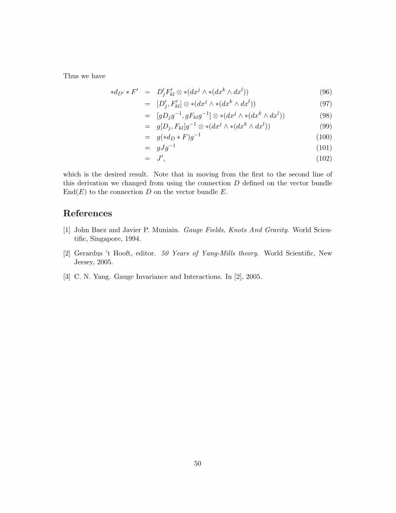
Thus we have

∗dD′ ∗ F ′ = D′jF

′kl ⊗ ∗(dxj ∧ ∗(dxk ∧ dxl)) (96)

= [D′j , F

′kl]⊗ ∗(dxj ∧ ∗(dxk ∧ dxl)) (97)

= [gDjg−1, gFklg

−1]⊗ ∗(dxj ∧ ∗(dxk ∧ dxl)) (98)= g[Dj , Fkl]g−1 ⊗ ∗(dxj ∧ ∗(dxk ∧ dxl)) (99)= g(∗dD ∗ F )g−1 (100)= gJg−1 (101)= J ′, (102)

which is the desired result. Note that in moving from the first to the second line ofthis derivation we changed from using the connection D defined on the vector bundleEnd(E) to the connection D on the vector bundle E.

References

[1] John Baez and Javier P. Muniain. Gauge Fields, Knots And Gravity. World Scien-tific, Singapore, 1994.

[2] Gerardus ’t Hooft, editor. 50 Years of Yang-Mills theory. World Scientific, NewJersey, 2005.

[3] C. N. Yang. Gauge Invariance and Interactions. In [2], 2005.

50