Embed Size (px)
Citation preview

Amplitudes in Yang-Mills theory and gravity
Stefan Weinzierl
Institut fur Physik, Universitat Mainz
I. Scattering amplitudes
II. Review of recent developments
III. Geometric interpretation of scattering amplitudes

Detailed outline
I. Scattering amplitudes
- The zeroth copy: Bi-adjoint scalar theory
- The single copy: Yang-Mills theory
- The double copy: Gravity
II. Review of recent developments
- Jacobi-like relations (BCJ numerators)
- The scattering equations (CHY representation)
- KLT relations
- Positive geometries and canonical forms
- Intersection theory
III. Geometric interpretation of scattering amplitudes

Part I
Scattering amplitudes

Amplitudes
In this talk we are interested in amplitudes of the following theories:
The zeroth copy: Bi-adjoint scalar theory
The single copy: Yang-Mills theory
The double copy: Gravity
We consider tree amplitudes with an arbitrary number of external particles n.

The single copy: Yang-Mills theory
The Lagrangian of a non-Abelian gauge theory:
LYM = −1
4Fa
µνFaµν, Faµν = ∂µAa
ν−∂νAaµ+g f abcAb
µAcν
Decompose the tree amplitudes An(p,ε) into group-theoretical factors and cyclic-
ordered amplitudes An(σ, p,ε):
An (p,ε) = gn−2 ∑σ∈Sn/Zn
2 Tr(T aσ(1)...T aσ(n)) An (σ, p,ε)
with
p = (p1, ..., pn) momenta
ε = (ε1, ...,εn) polarisations
σ = (σ1, ...,σn) cyclic order

Colour decomposition
Lie algebra:
[
T a,T b]
= i f abcT c, Tr(
T aT b)
=1
2δab
Multiply commutator relation by T d and take the trace:
i f abc = 2Tr(
T aT bT c)
−2Tr(
T bT aT c)
Fierz identities for U(N):
Tr(T aX)Tr(T aY ) =1
2Tr(XY ) , Tr(T aXT aY ) =
1
2Tr(X)Tr(Y )

Primitive amplitudes
The primitive amplitudes are gauge-invariant and each primitive amplitude has a fixed
cyclic order of the external legs.
The primitive amplitudes are calculated from cyclic-ordered Feynman rules:
= −igµν
p2
= i [gµ1µ2 (pµ3
1− p
µ3
2)+gµ2µ3 (p
µ1
2− p
µ1
3)+gµ3µ1 (p
µ2
3− p
µ2
1)]
= i [2gµ1µ3gµ2µ4 −gµ1µ2gµ3µ4 −gµ1µ4gµ2µ3]

The zeroth copy: Bi-adjoint scalar theory
A scalar field in the adjoint representation of two gauge-groups G× G with Lagrange
density
L =1
2
(
∂µφab)(
∂µφab)
− λ
3!f a1a2a3 f b1b2b3φa1b1φa2b2φa3b3
Decompose the tree amplitudes mn(p) into group-theoretical factors and double-
ordered amplitudes mn(σ, σ, p):
mn (p) = λn−2 ∑σ∈Sn/Zn
∑σ∈Sn/Zn
2 Tr(T aσ(1)...T aσ(n)) 2 Tr(
T bσ(1)...T bσ(n)
)
mn (σ, σ, p)
The permutations σ and σ denote two cyclic orders.

Double-ordered amplitudes
Flip: exchange two branches at a vertex.
1 2 3 4
5
⇔1 4 2 3
5
Two diagrams with different external orders are equivalent, if we can transform one
diagram into the other by a sequence of flips.
The double-ordered amplitude mn(σ, σ, p) is computed from the Feynman diagrams
compatible with the cyclic orders σ and σ.
Feynman rules:
=i
p2
= i

The double copy: Gravity
Let us consider (small) fluctuations around the flat Minkowski metric
gµν = ηµν+κhµν,
with κ =√
32πG and consider an effective theory defined by the Einstein-Hilbert
Lagrangian
LEH = − 2
κ2
√−gR.
The field hµν describes a graviton.
The inverse metric gµν and√−g are infinite series in hµν, therefore
LEH+LGF =∞
∑n=2
L(n),
where L(n) contains exactly n fields hµν.
Thus the Feynman rules will give an infinite tower of vertices.

Feynman rules for gravity
External edge:
µ1,µ2 = εµ1(k)εµ2
(k)
Internal edge:
µ1,µ2 ν1,ν2 =1
2
(
ηµ1ν1ηµ2ν2
+ηµ1ν2ηµ2ν1
− 2
D−2ηµ1µ2
ην1ν2
)
i
k2
Vertices:
= long expression
= even longer expression
plus Feynman rules for 5-graviton vertex, 6-graviton vertex, etc.
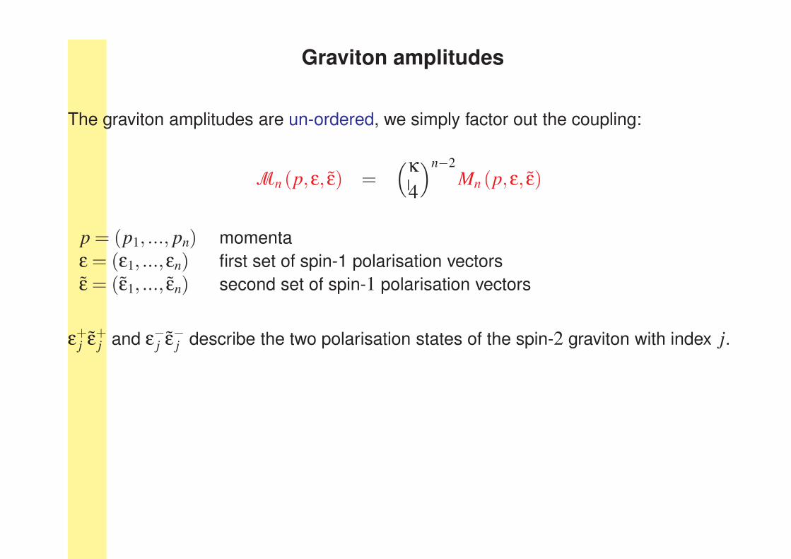
Graviton amplitudes
The graviton amplitudes are un-ordered, we simply factor out the coupling:
Mn (p,ε, ε) =(κ
4
)n−2
Mn (p,ε, ε)
p = (p1, ..., pn) momenta
ε = (ε1, ...,εn) first set of spin-1 polarisation vectors
ε = (ε1, ..., εn) second set of spin-1 polarisation vectors
ε+j ε+j and ε−j ε−j describe the two polarisation states of the spin-2 graviton with index j.

Amplitudes
We consider the double ordered bi-adjoint scalar amplitudes mn(σ, σ, p), the single
ordered Yang-Mills amplitudes An(σ, p,ε) and the un-ordered graviton amplitudes
Mn(p,ε, ε).
All these amplitudes can be computed from Feynman diagrams.
mn (σ, σ, p) = i(−1)n−3+nflip(σ,σ) ∑trivalent graphs G
compatible with σ and σ
1
D(G), D(G) = ∏
edges e
se,
An (σ, p,ε) = long expression,
Mn (p,ε, ε) = even longer expression.

Part II
Review of recent developments
1. Jacobi-like relations (BCJ numerators)
2. The scattering equations (CHY representation)
3. KLT relations
4. Positive geometries and canonical forms
5. Intersection theory

Part II.1
Jacobi-like relations

Jacobi relation
Jacobi relation:
[[
T a,T b]
,T c]
+[[
T b,T c]
,T a]
+[
[T c,T a] ,T b]
= 0,
In terms of structure constants:
(
i f abe)(
i f ecd)
+(
i f bce)(
i f ead)
+(i f cae)(
i f ebd)
= 0.
Graphically:
1 2 3
4
+
2 3 1
4
+
3 1 2
4
= 0

Expansion in graphs with three-valent vertices only
In Yang-Mills theory we have a three-valent and a four-valent vertex.
We may always re-write a four-valent vertex in terms of two three-valent vertices:
1
2 3
4
=
1
2 3
4
+
1
2 3
4
This is not unique!

BCJ numerators
We may write the Yang-Mills amplitude in a form
An (σ, p,ε) = i(−1)n−3 ∑trivalent graphs G
with order σ
N(G)
D(G),
with numerators N(G) satisfying anti-symmetry relations and Jacobi relations:
1 2 3
4
+
2 3 1
4
+
3 1 2
4
= 0
N (G1) + N (G2) + N (G3) = 0
Bern, Carrasco, Johansson, ’10
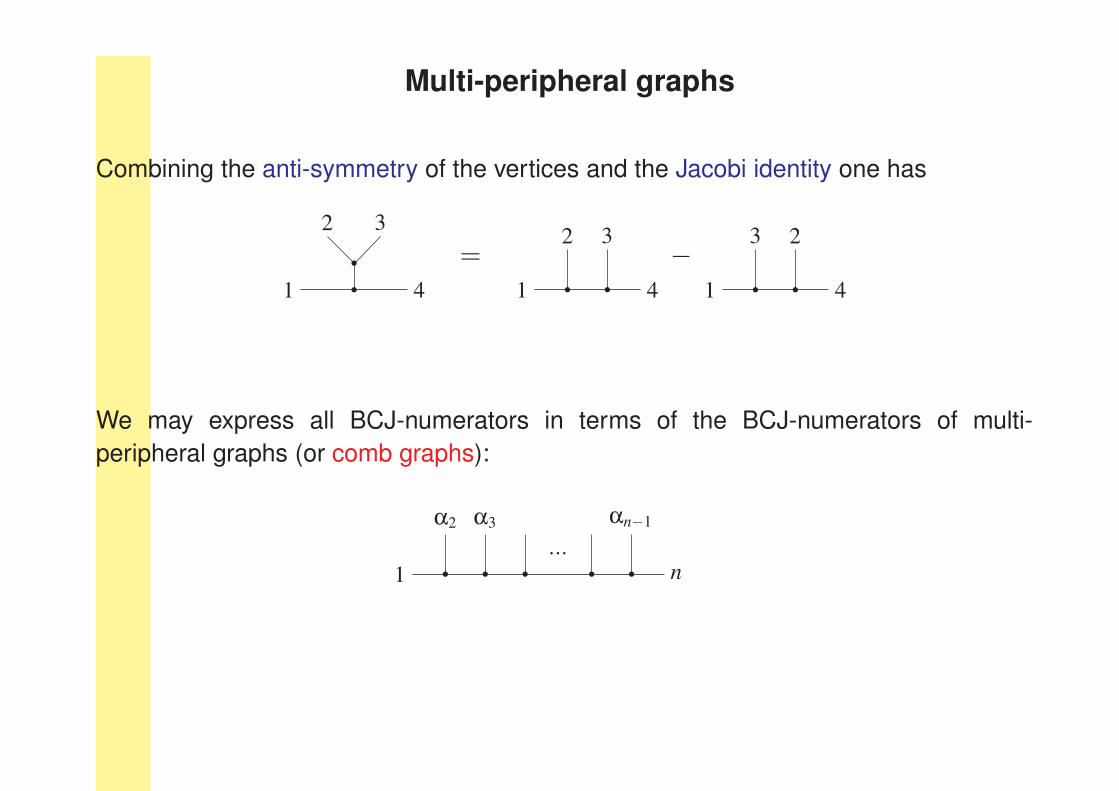
Multi-peripheral graphs
Combining the anti-symmetry of the vertices and the Jacobi identity one has
1
2 3
4
=1
2 3
4
−1
3 2
4
We may express all BCJ-numerators in terms of the BCJ-numerators of multi-
peripheral graphs (or comb graphs):
1
α2 α3
...
αn−1
n

Double copy and colour-kinematics duality
If the Yang-Mills amplitude is written in terms of BCJ-numerators N(G) and group-
theoretical factors C(G)
An (p,ε) = i(−1)n−3gn−2 ∑
trivalent graphs G
C (G)N (G)
D(G),
then
Mn (p,ε, ε) = i(−1)n−3
(κ
4
)n−2
∑trivalent graphs G
N (G)N (G)
D(G),
and of course
mn (p) = i(−1)n−3 λn−2 ∑trivalent graphs G
C (G)C (G)
D(G).
Bern, Carrasco, Johansson, ’10

Effective Lagrangian
We may construct an effective Lagrangian, which gives directly BCJ-numerators
LYM+LGF =∞
∑n=2
L(n),
L(2), L(3) and L(4) agree with the standard terms and L(n≥5) are a complicated zero.
The effective Lagrangian is not unique.
Tolotti, S.W, ’13

Part II.2
The scattering equations

The Riemann sphere
The Riemann sphere is the complex plane plus the point at infinity:
C = C∪∞
Each g =
(
a b
c d
)
∈ PSL(2,C) acts on z ∈ C through a Mobius transformation:
g · z =az+b
cz+d.
Mark n distinct points (z1, ...,zn) on C.
The moduli space of genus 0 curves with n distinct marked points is denoted by
M0,n =
z ∈ Cn
: zi 6= z j
/PSL(2,C) .
M0,n is an affine algebraic variety of dimension (n−3).

The scattering equations
Set
fi (z, p) =n
∑j=1, j 6=i
2pi · p j
zi− z j
.
The scattering equations:
fi (z, p) = 0, 1 ≤ i ≤ n.
Only (n−3) equations of the n equations are independent.
Two solutions which are related by a Mobius-transformation are called equivalent
solutions.
There are (n−3)! inequivalent solutions not related by a Mobius-transformation.

The CHY representation
There exists two functions C(σ,z) and E(p,ε,z) on Cn such that
mn (σ, σ, p) = i
∮
C
dΩCHY C (σ,z)C (σ,z),
An (σ, p,ε) = i
∮
C
dΩCHY C (σ,z) E (p,ε,z),
Mn (p,ε, ε) = i
∮
C
dΩCHY E (p,ε,z) E (p, ε,z).
Details on the definition of the measure dΩCHY:
dΩCHY =1
(2πi)n−3
dnz
dω ∏ ′ 1
fa (z, p), ∏ ′ 1
fa (z, p)= (−1)i+ j+k
(
zi− z j
)(
z j − zk
)
(zk − zi) ∏a6=i, j,k
1
fa (z, p),
dω = (−1)p+q+r dzpdzqdzr(
zp− zq
)(
zq− zr
)(
zr − zq
) .
Cachazo, He and Yuan, ’13

The cyclic factor
The cyclic factor (or Parke-Taylor factor) is given by
C (σ,z) =1
(zσ1− zσ2
)(zσ2− zσ3
) ...(zσn − zσ1).
The cyclic factor encodes the information on the cyclic order.

The polarisation factor
The polarisation factor E (p,ε,z) encodes the information on the helicities of the
external particles.
One possibility to define this factor is through a reduced Pfaffian.
(All definitions have to agree on the solutions of the scattering equations, but may differ
away from this zero-dimensional sub-variety.)

The reduced Pfaffian
Define a (2n)× (2n) antisymmetric matrix Ψ(z, p,ε) through
Ψ(z, p,ε) =
(
A −CT
C B
)
with
Aab =
2pa·pb
za−zba 6= b,
0 a = b,Bab =
2εa·εb
za−zba 6= b,
0 a = b,Cab =
2εa·pb
za−zba 6= b,
−n
∑j=1, j 6=a
2εa·p j
za−z ja = b.
Denote by Ψi ji j the (2n− 2)× (2n− 2)-matrix, where rows and columns i and j have
been deleted (1 ≤ i < j ≤ n).
The reduced Pfaffian EPfaff(z, p,ε) is defined by
EPfaff (z, p,ε) =(−1)i+ j
2(zi− z j)Pf Ψi j
i j (z, p,ε) .
Cachazo, He and Yuan, ’13
Part II.3
KLT relations

Independent primitive amplitudes
How many independent primitive amplitudes An(σ, p,ε) are there for fixed momenta p
and polarisations ε ?
• There are n! external orderings.
• Cyclic invariance reduce the number to (n−1)!.
• Anti-symmetry of the vertices reduce the number to (n−2)!.Kleiss, Kuijf, 1989
• Jacobi relations reduce the number to (n−3)!.Bern, Carrasco, Johansson, 2008
Basis B of independent amplitudes consists of (n−3)! elements.

KLT relations
Define (n−3)!× (n−3)!-dimensional matrix mσσ for σ, σ ∈ B by
mσσ = mn (σ, σ, p) .
The matrix m is invertible.
Define the KLT-matrix as the inverse of the matrix m:
S = m−1
Kawai, Lewellen, Tye, 1986,
Bjerrum-Bohr, Damgaard, Sondergaard, Vanhove, 2010,
Cachazo, He and Yuan, 2013,
de la Cruz, Kniss, S.W., 2016

KLT relations
The KLT relations express the graviton amplitude Mn(p,ε, ε) through products of Yang-
Mills amplitudes An(σ, p,ε) and the KLT-matrix S:
Mn (p,ε, ε) = ∑σ,σ∈B
An (σ, p,ε) Sσσ An (σ, p, ε)
Graphically:
=

Part II.4
Positive geometries and canonical forms

Multivariate residues of differential forms
Let X be a m-dimensional variety and Y a co-dimension one sub-variety.
Let us choose a coordinate system such that Y is given locally by z1 = 0.
Assume that Ω has a pole of order 1 on Y :
Ω =dz1
z1
∧ψ+θ.
The residue of Ω at Y is defined by
ResY (Ω) = ψ|Y .
A pole of order 1 on Y is called a logarithmic singularity on Y .

Positive geometries and canonical forms
Let X be a m-dimensional (complex) variety and X≥0 the positive part.
A m-form Ω is called a canonical form if
1. For m = 0 one has Ω =±1.
2. The only singularities of Ω are on the boundary of X≥0.
3. The singularities are logarithmic.
4. The residue of Ω on a boundary component is again the canonical form of a (m−1)-dimensional positive geometry.
Arkani-Hamed, Bai, Lam, ’17

Part II.5
Intersection theory

The CHY representation
The CHY half-integrands C(σ,z) and E(p,ε,z) transform under PSL(2,C)-transformations as
F (g · z) =
(
n
∏j=1
(cz j +d)2
)
F (z)
Therefore, the (n−3)-forms
Ωcyclic (σ,z) = C (σ,z)dnz
dω, Ωpol (p,ε,z) = E (p,ε,z)
dnz
dω.
are PSL(2,C)-invariant.
Remark: We may add to C(σ,z) and E(p,ε,z) terms which vanish on the solutions of
the scattering equations.

Intersection theory
Consider a space X of dimension m, equipped with a connection ∇ = d +η.
The connection one-form η is called the twist.
Elements of
Hm (X ,∇) = ϕ | ∇ϕ = 0 / ∇ξ
are called twisted co-cycles.
The intersection number of two twisted co-cycles is defined by
(ϕ1,ϕ2) =1
(2πi)m
∫
X
ι(ϕ1)∧ϕ2,
where ι maps ϕ1 to a twisted co-cycle in the same cohomology class but with compact
support.
Cho, Matsumoto, ’95; Aomoto, Kita, ’94 (jap.), ’11 (engl.)
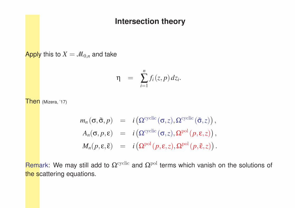
Intersection theory
Apply this to X =M0,n and take
η =n
∑i=1
fi (z, p)dzi.
Then (Mizera, ’17)
mn (σ, σ, p) = i(
Ωcyclic (σ,z),Ωcyclic (σ,z))
,
An(σ, p,ε) = i(
Ωcyclic (σ,z),Ωpol (p,ε,z))
,
Mn(p,ε, ε) = i(
Ωpol (p,ε,z),Ωpol (p, ε,z))
.
Remark: We may still add to Ωcyclic and Ωpol terms which vanish on the solutions of
the scattering equations.

Part III
Geometric interpretation of scattering amplitudes

Geometric interpretation of tree amplitudes
There exist two (n−3)-forms Ωcyclic(σ,z) and Ωpol(p,ε,z) on the compactified moduli
space M0,n such that
1. The twisted intersection numbers give the amplitudes for the bi-adjoint
scalar theory (cyclic, cyclic), Yang-Mills theory (cyclic,polarisation) and gravity
(polarisation,polarisation).
2. The only singularities of the scattering forms are on the divisor M0,n\M0,n.
3. The singularities are logarithmic.
4. The residues at the singularities factorise into two scattering forms of lower points.
L. de la Cruz, A. Kniss, S.W., ’17

The scattering forms
The cyclic scattering form is defined by
Ωcyclic (σ,z) = C (σ,z)dnz
dω, C (σ,z) =
1
(zσ1− zσ2
)(zσ2− zσ3
) ...(zσn − zσ1).
The polarisation scattering form is defined by
Ωpol (p,ε,z) = E (p,ε,z)dnz
dω, E (p,ε,z) = ∑
κ∈S(1,n)n−2
C (κ,z) Ncomb (κ) ,
where the sum is now over all permutations keeping κ1 = 1 and κn = n fixed.
L. de la Cruz, A. Kniss, S.W., ’17

Wrap-up
The n-graviton amplitude is given by
Mn (p,ε, ε) = i(−1)n−3 ∑trivalent graphs G
N (G) N (G)
D(G)colour-kinematics duality
= i
∮
C
dΩCHY E (p,ε,z) E (p, ε,z) CHY representation
= ∑σ,σ∈B
An (σ, p,ε) Sσσ An (σ, p, ε) KLT relation
= i(
Ωpol (p,ε,z) ,Ωpol (p, ε,z))
intersection number

References
• Jacobi-like relations
– Z. Bern, J.J. Carrasco, H. Johansson New Relations for Gauge-Theory Amplitudes, Phys.Rev.D78, (2008), 085011,
arXiv:0805.3993
– Z. Bern, J.J. Carrasco, H. Johansson Perturbative Quantum Gravity as a Double Copy of Gauge Theory,
Phys.Rev.Lett. 105, (2010), 061602, arXiv:1004.476
• The scattering equations
– F. Cachazo, S. He, E. Y. Yuan, Scattering of Massless Particles in Arbitrary Dimension, Phys.Rev.Lett. 113, (2014),
171601, arXiv:1307.2199
– F. Cachazo, S. He, E. Y. Yuan, Scattering of Massless Particles: Scalars, Gluons and Gravitons, JHEP 1407, (2014),
033, arXiv:1309.0885
• Positive geometries and canonical forms
– N. Arkani-Hamed, Y. Bai, T. Lam, Positive Geometries and Canonical Forms, JHEP 1711, (2017), 039,
arXiv:1703.04541
– N. Arkani-Hamed, Y. Bai, T. Lam, Scattering Forms and the Positive Geometry of Kinematics, Color and the
Worldsheet, JHEP 1805, (2018), 096, arXiv:1711.09102
• Intersection theory
– S. Mizera, Combinatorics and Topology of Kawai-Lewellen-Tye Relations, JHEP 1708, (2017), 097, arXiv:1706.08527
– S. Mizera, Scattering Amplitudes from Intersection Theory, Phys.Rev.Lett. 120, (2018), 141602, arXiv:1711.00469
• ... and some self-advertisement
– S. Weinzierl, Tales of 1001 Gluons, Phys.Rept. 676, (2017), 1, arXiv:1610.05318
– L. de la Cruz, A. Kniss, S. Weinzierl, Properties of scattering forms and their relation to associahedra, JHEP 1803,
(2018), 064, arXiv:1711.07942

Concluding controversial statement
There are interesting relations between the (tree-level) scattering amplitudes of Yang-
Mills theory and gravity.
These relations are not manifest in the action as a coordinate space integral over a
Lagrange density.
Should we not find and work with a formulation, which makes these structures manifest
from the beginning?


![City Research Onlineof encoding scattering amplitudes in N= 4 super-Yang-Mills theory in terms of planar bipartite graphs and cells in the positive Grassmannian [17{21]. Amongst these](https://img.pdfslide.us/doc/110x75/5f0873497e708231d4221295/city-research-online-of-encoding-scattering-amplitudes-in-n-4-super-yang-mills.jpg)