4NoiseinCommunicationSystems · 84 4 Noise in Communication Systems 4.2.1 Time-Averaged Noise Representations Informing averages of any signal, whether random or deterministic, weﬁndparameters

4 Noise in Communication Systems

4.1 Definition of Noise

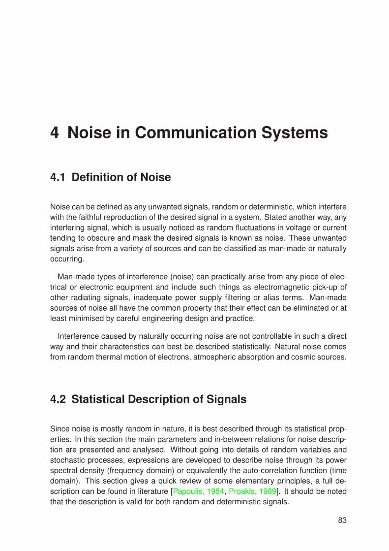
Noise can be defined as any unwanted signals, random or deterministic, which interferewith the faithful reproduction of the desired signal in a system. Stated another way, anyinterfering signal, which is usually noticed as random fluctuations in voltage or currenttending to obscure and mask the desired signals is known as noise. These unwantedsignals arise from a variety of sources and can be classified as man-made or naturallyoccurring.

Man-made types of interference (noise) can practically arise from any piece of elec-trical or electronic equipment and include such things as electromagnetic pick-up ofother radiating signals, inadequate power supply filtering or alias terms. Man-madesources of noise all have the common property that their effect can be eliminated or atleast minimised by careful engineering design and practice.

Interference caused by naturally occurring noise are not controllable in such a directway and their characteristics can best be described statistically. Natural noise comesfrom random thermal motion of electrons, atmospheric absorption and cosmic sources.

4.2 Statistical Description of Signals

Since noise is mostly random in nature, it is best described through its statistical prop-erties. In this section the main parameters and in-between relations for noise descrip-tion are presented and analysed. Without going into details of random variables andstochastic processes, expressions are developed to describe noise through its powerspectral density (frequency domain) or equivalently the auto-correlation function (timedomain). This section gives a quick review of some elementary principles, a full de-scription can be found in literature [Papoulis, 1984, Proakis, 1989]. It should be notedthat the description is valid for both random and deterministic signals.

83

84 4 Noise in Communication Systems

4.2.1 Time-Averaged Noise Representations

In forming averages of any signal, whether random or deterministic, we find parameterswhich tell us something about the signal. But much of the detailed information aboutthe signal is lost through this process. In the case of random noise, however, this is theonly useful quantity.

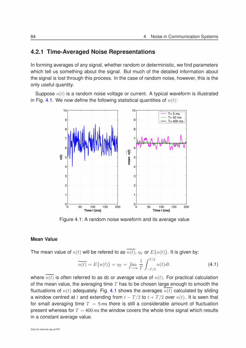
Suppose n(t) is a random noise voltage or current. A typical waveform is illustratedin Fig. 4.1. We now define the following statistical quantities of n(t):

0 50 100 150 2000

1

2

3

4

5

6

7

8

9

10

Time t [ms]

n(t)

0 50 100 150 2000

1

2

3

4

5

6

7

8

9

10

Time t [ms]

_

__m

ean

n(t)

T= 5 ms T= 50 ms T= 400 ms

Figure 4.1: A random noise waveform and its average value

Mean Value

The mean value of n(t) will be refered to as n(t), ηT or En(t). It is given by:

n(t) = En(t) = ηT = limT→∞

1

T

! T/2

−T/2

n(t)dt. (4.1)

where n(t) is often referred to as dc or average value of n(t). For practical calculationof the mean value, the averaging time T has to be chosen large enough to smooth thefluctuations of n(t) adequately. Fig. 4.1 shows the averages n(t) calculated by slidinga window centred at t and extending from t − T/2 to t + T/2 over n(t). It is seen thatfor small averaging time T = 5ms there is still a considerable amount of fluctuationpresent whereas for T = 400ms the window covers the whole time signal which resultsin a constant average value.

Only for internal use at KIT

4.2 Statistical Description of Signals 85

Mean-Square Value

n2(t) = En2(t) = limT→∞

1

T

! T/2

−T/2

|n(t)|2dt. (4.2)

Aside from a scaling factor the mean-square value n2(t) in (4.2) gives the time av-eraged power P of n(t). Assuming n(t) to be the noise voltage or current, the scalingfactor will be equivalent to a resistance, which is often set equal to 1Ω. The squareroot of n2(t) is known as the root-mean-square (rms) value of n(t). The advantage of

the rms notation is that the units of"

n2(t) are the same as those for n(t).

AC Component

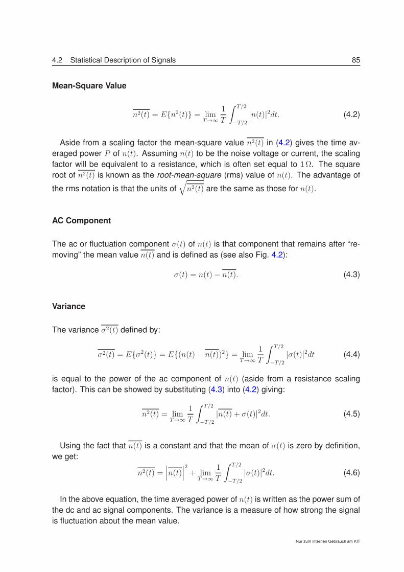
The ac or fluctuation component σ(t) of n(t) is that component that remains after “re-moving” the mean value n(t) and is defined as (see also Fig. 4.2):

σ(t) = n(t)− n(t). (4.3)

Variance

The variance σ2(t) defined by:

σ2(t) = Eσ2(t) = E(n(t)− n(t))2 = limT→∞

1

T

! T/2

−T/2

|σ(t)|2dt (4.4)

is equal to the power of the ac component of n(t) (aside from a resistance scalingfactor). This can be showed by substituting (4.3) into (4.2) giving:

n2(t) = limT→∞

1

T

! T/2

−T/2

|n(t) + σ(t)|2dt. (4.5)

Using the fact that n(t) is a constant and that the mean of σ(t) is zero by definition,we get:

n2(t) =###n(t)

###2+ lim

T→∞

1

T

! T/2

−T/2

|σ(t)|2dt. (4.6)

In the above equation, the time averaged power of n(t) is written as the power sum ofthe dc and ac signal components. The variance is a measure of how strong the signalis fluctuation about the mean value.

Nur zum internen Gebrauch am KIT


0 50 100 150 200−3

−2

−1

0

1

2

3

4

5

6

7

Time t [ms]

AC

com

pone

nt σ

(t)

0 50 100 150 200−3

−2

−1

0

1

2

3

4

5

6

7

Time t [ms]

_

___

varia

nce

σ 2 (t)

T= 5 ms T= 50 ms T= 400 ms

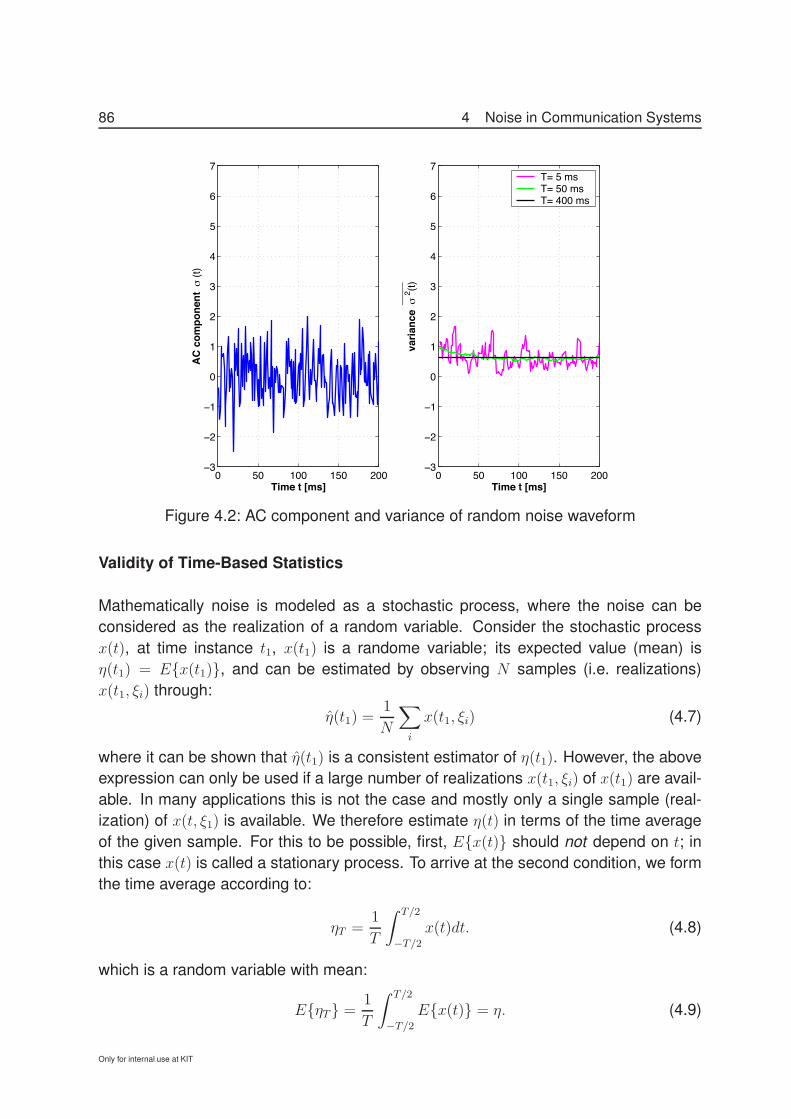
Figure 4.2: AC component and variance of random noise waveform

Validity of Time-Based Statistics

Mathematically noise is modeled as a stochastic process, where the noise can beconsidered as the realization of a random variable. Consider the stochastic processx(t), at time instance t1, x(t1) is a randome variable; its expected value (mean) isη(t1) = Ex(t1), and can be estimated by observing N samples (i.e. realizations)x(t1, ξi) through:

η(t1) =1

N

$

i

x(t1, ξi) (4.7)

where it can be shown that η(t1) is a consistent estimator of η(t1). However, the aboveexpression can only be used if a large number of realizations x(t1, ξi) of x(t1) are avail-able. In many applications this is not the case and mostly only a single sample (real-ization) of x(t, ξ1) is available. We therefore estimate η(t) in terms of the time averageof the given sample. For this to be possible, first, Ex(t) should not depend on t; inthis case x(t) is called a stationary process. To arrive at the second condition, we formthe time average according to:

ηT =1

T

! T/2

−T/2

x(t)dt. (4.8)

which is a random variable with mean:

EηT =1

T

! T/2

−T/2

Ex(t) = η. (4.9)



Now if the time average ηT computed from a single realization of x(t) tends to theensemble average η as T → ∞ then the random process is called mean-ergodic.

As such, for ergodic random processes a single time realization can be used to obtainthe moments of the process. Thus, the expressions in (4.1) to (4.6) are only correct ifthe stochastic process is both stationary and ergodic [Papoulis, 1984, Proakis, 1989].In addition, since the measuring time T is finite the quantities are only estimated valuesof the moments. In practice, the only quantity accessible to measurements is n(t),which forces us to assume a stationary, ergodic stochastic process.

Drill Problem 33 Calculate the (a) average value, (b) ac component, and (c) rms valueof the periodic waveform v(t) = 1 + 3 cos(2πft).

Drill Problem 34 A voltage source generating the waveform of drill problem 33 is con-nected to a resistor R = 6Ω. What is the power dissipated in the resistor?

4.2.2 Fourier Transform

The definition of the Fourier transform [Stremler, 1982] is given by

F (f) = Ff(t) =

! ∞

−∞f(t)e−j2πftdt (4.10)

and the inverse Fourier transform

f(t) = F−1F (f) =

! ∞

−∞F (f)ej2πftdf. (4.11)

If the signal f(t) is a power signal, i.e., a signal with finite power but infinite energy,the integral in (4.10) will diverge. However, considering the practical case of a finiteobservation time T and assume that the signal is zero outside this interval, is equivalentto multiplying the signal by the unit gate function rect(t/T ). In this case the Fouriertransform can be written as:

FT (f) = Ff(t)rect(t/T ) =

! T/2

−T/2

f(t)e−j2πftdt (4.12)

Note that the multiplication by the rect-function in the time domain is equivalent to aconvolution by a sinc-function in the frequency domain.

4.2.3 Correlation Functions

In the following, two statistical functions are introduced which can be used to investigatethe similarity between random functions.



Auto-Correlation Function

The auto-correlation function Ef ∗(t)f(t + τ) = Rf (τ) of a signal f(t) is defined as[Stremler, 1982]:

Ef ∗(t)f(t+ τ) = Rf (τ) = limT→∞

1

T

! T/2

−T/2

f ∗(t)f(t+ τ)dt (4.13)

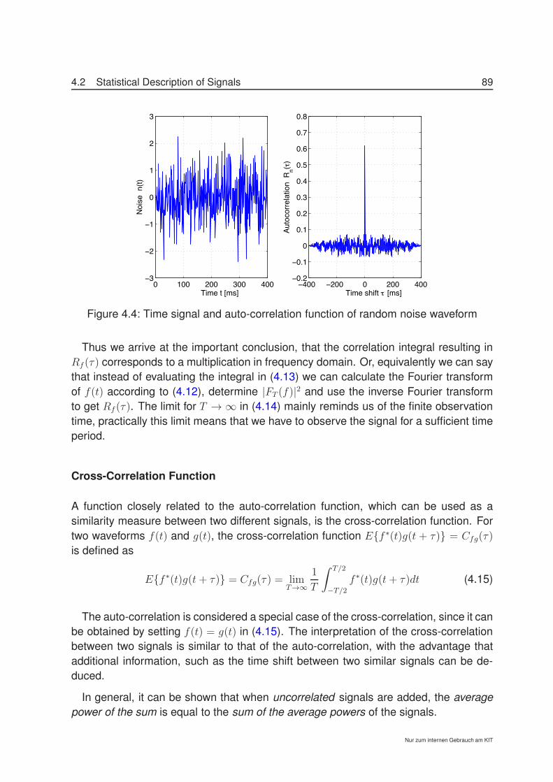
where f ∗(t) is the complex conjugate of f(t). Note that the subscript f is added tothe autocorrelation funciton R(τ) to indicate the random variable or function that isconsidered. The auto-correlation function (4.13) is often used in signal analysis, itgives a similarity measure of the signal f(t) with itself versus a relative time shift byan amount τ . For slowly varying time signals, the signal values doesn’t change rapidlyover time which will result in a flat auto-correlation function Rf(τ). Noise signals on theother hand, tend to have rapid fluctuations giving rise to an auto-correlation functionwith a sharp peak for τ = 0 (no time shift) and quickly falling to zero for increasing τ .As an example Figs. 4.3 and 4.4 show the time signals and the corresponding auto-correlation functions for both an exponential and a random noise signal.

0 100 200 300 4000

0.2

0.4

0.6

0.8

1

1.2

1.4

1.6

1.8

2

Time t [ms]

Sign

al s

(t)

−400 −200 0 200 400−0.1

0

0.1

0.2

0.3

0.4

0.5

Time shift [ms]τ

Auto

corre

latio

n R

s(τ)

Figure 4.3: Time signal and auto-correlation function of exponential waveform

When dealing with random variables, the auto-correlation function Rf (τ) is a statisti-cal quantity describing the stochastic process. Note that setting τ = 0 in (4.13) yieldsRf (0) = Ef 2(t) = f 2(t) which is the average power of the signal as is readily seenby comparing to (4.2). Again, we note that the definition of Rf (τ) as given by (4.13) isonly valid if the stochastic process is both stationary and ergodic.

It can be shown, that taking the Fourier transform (with respect to τ ) of both sides of(4.13) yields [Proakis, 1989]:

FτRf(τ) = limT→∞

1

TF ∗T (f)FT (f) = lim

T→∞

1

T|FT (f)|2 (4.14)



0 100 200 300 400−3

−2

−1

0

1

2

3

Time t [ms]

Noi

se n

(t)

−400 −200 0 200 400−0.2

−0.1

0

0.1

0.2

0.3

0.4

0.5

0.6

0.7

0.8

Time shift [ms]τAu

toco

rrela

tion

Rn(τ

)

Figure 4.4: Time signal and auto-correlation function of random noise waveform

Thus we arrive at the important conclusion, that the correlation integral resulting inRf (τ) corresponds to a multiplication in frequency domain. Or, equivalently we can saythat instead of evaluating the integral in (4.13) we can calculate the Fourier transformof f(t) according to (4.12), determine |FT (f)|2 and use the inverse Fourier transformto get Rf (τ). The limit for T → ∞ in (4.14) mainly reminds us of the finite observationtime, practically this limit means that we have to observe the signal for a sufficient timeperiod.

Cross-Correlation Function

A function closely related to the auto-correlation function, which can be used as asimilarity measure between two different signals, is the cross-correlation function. Fortwo waveforms f(t) and g(t), the cross-correlation function Ef ∗(t)g(t + τ) = Cfg(τ)is defined as

Ef ∗(t)g(t+ τ) = Cfg(τ) = limT→∞

1

T

! T/2

−T/2

f ∗(t)g(t+ τ)dt (4.15)

The auto-correlation is considered a special case of the cross-correlation, since it canbe obtained by setting f(t) = g(t) in (4.15). The interpretation of the cross-correlationbetween two signals is similar to that of the auto-correlation, with the advantage thatadditional information, such as the time shift between two similar signals can be de-duced.

In general, it can be shown that when uncorrelated signals are added, the averagepower of the sum is equal to the sum of the average powers of the signals.



0 100 200 300 400−2

−1

0

1

2

3

4

Time t [ms]

g(t)=

s(t)+

n(t)

−400 −200 0 200 400

0

0.2

0.4

0.6

0.8

1

1.2

Time shift [ms]τAu

toco

rrela

tion

Rg(τ

)

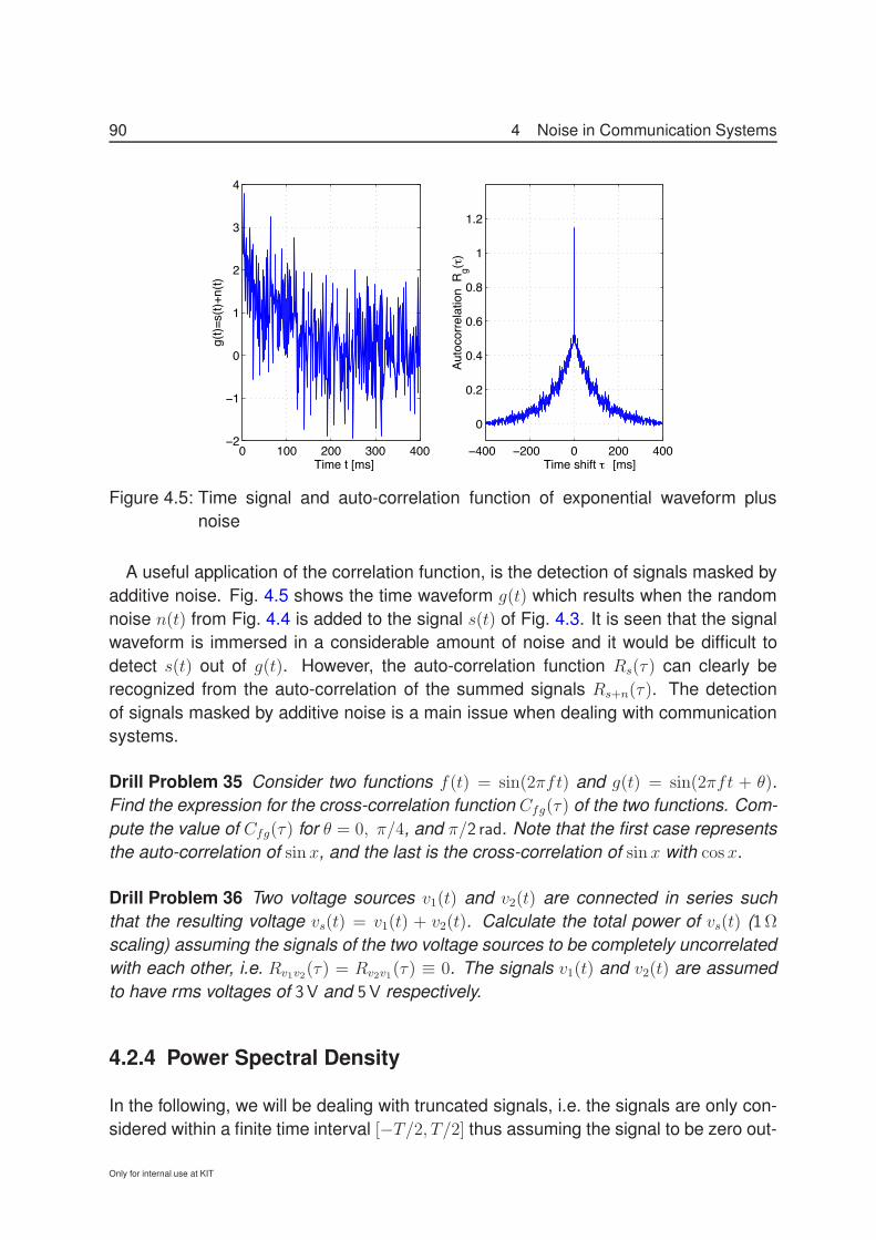
Figure 4.5: Time signal and auto-correlation function of exponential waveform plusnoise

A useful application of the correlation function, is the detection of signals masked byadditive noise. Fig. 4.5 shows the time waveform g(t) which results when the randomnoise n(t) from Fig. 4.4 is added to the signal s(t) of Fig. 4.3. It is seen that the signalwaveform is immersed in a considerable amount of noise and it would be difficult todetect s(t) out of g(t). However, the auto-correlation function Rs(τ) can clearly berecognized from the auto-correlation of the summed signals Rs+n(τ). The detectionof signals masked by additive noise is a main issue when dealing with communicationsystems.

Drill Problem 35 Consider two functions f(t) = sin(2πft) and g(t) = sin(2πft + θ).Find the expression for the cross-correlation function Cfg(τ) of the two functions. Com-pute the value of Cfg(τ) for θ = 0, π/4, and π/2 rad. Note that the first case representsthe auto-correlation of sin x, and the last is the cross-correlation of sin x with cosx.

Drill Problem 36 Two voltage sources v1(t) and v2(t) are connected in series suchthat the resulting voltage vs(t) = v1(t) + v2(t). Calculate the total power of vs(t) (1Ωscaling) assuming the signals of the two voltage sources to be completely uncorrelatedwith each other, i.e. Rv1v2(τ) = Rv2v1(τ) ≡0. The signals v1(t) and v2(t) are assumedto have rms voltages of 3 V and 5 V respectively.

4.2.4 Power Spectral Density

In the following, we will be dealing with truncated signals, i.e. the signals are only con-sidered within a finite time interval [−T/2, T/2] thus assuming the signal to be zero out-



side this interval. The mathematical representation is not as strait forward as for infinitetime signals, however, practical consideration show that this extra effort is needed.Parseval’s theorem for truncated signals state that:

! T/2

−T/2

|f(t)|2dt =! ∞

−∞|FT (f)|2df. (4.16)

Noting the similarity between the first term in (4.16) and the time averaged power Pof a signal as given in (4.2) we write:

P = limT→∞

1

T

! T/2

−T/2

|f(t)|2dt = limT→∞

1

T

! ∞

−∞|FT (f)|2df. (4.17)

The first integral in the equation above is easy to understand, it shows that in orderto obtain the total power of a signal we must add together the power contribution ofeach time increment, which is done through the integration over time t. Whether weare dealing with voltage or current is indifferent if we assume a 1Ω resistance. Weknow, that evaluating the integral over a finite time period, will give us the signal powerwithin this time. The first integral is thus also valid over each time interval. However,Parseval’s equation suggests a second procedure to calculate the total power, whichis performed in the frequency domain. The last term in (4.17) shows that the summa-tion of |F (f)|2 over all frequencies f will also result in the total power P . Defining apower spectral density function S(f) in units of Watts per Hz such that its integral overfrequency is equal to the total power, gives:

! ∞

−∞S(f)df = lim

T→∞

1

T

! ∞

−∞|FT (f)|2df. (4.18)

In addition, we insist that S(f) also gives the power over each frequency increment,which means that the integration of the power density function over a frequency range∆f will give the total power for this frequency interval. It can be shown, that undercertain conditions –which are fulfilled for most practical signals of interest– S(f) isrelated to |FT (f)|2 through:

S(f) = limT→∞

|FT (f)|2

T. (4.19)

Through (4.14) the relation between the power spectral density and the Fourier trans-form of the auto-correlation function is given:

S(f) = FRf(τ) (4.20)

When evaluating the distribution of noise power over frequency, the power spectraldensity S(f) should be the function to examine, rather then the Fourier transform. The



reason for this, is, that the Fourier transform of a random quantity (cf. the expressionin (4.12)) is also a random quantity, which in this sense does not give us any usefulinformation. As we know, for random signals we need to investigate the statistical prop-erties. Thus in case we are interested in the frequency content of noise, we computethe Fourier transform of the auto-correlation function as given in the expression above.

Using (4.17), (4.18) and (4.13) we get:

P = f 2(t) = limT→∞

1

T

! T/2

−T/2

|f(t)|2dt =! ∞

−∞S(f)df = Rf (0) (4.21)

The above expression can be used to calculate the total power using either the timedomain signal, the power spectral density function, or the auto-correlation function.Care must be taken, when the resistive scaling factor is not equal to 1Ω.

4.3 Noise in Linear Systems

When designing and characterizing communication systems, noise is an important pa-rameter which must be accounted for. In general, the different physical noise sourcesin addition to other man-made noise sources contribute to the total noise in the system.In the following, noise in linear time invariant (LTI) systems is investigated.

4.3.1 Band Limited White Noise

The power spectral density shall be used to describe noise. Knowing that randomnoise tends to have rapid fluctuations, we assume a noise voltage n(t) having theauto-correlation function:

Rn(τ) =No

2δ(τ) (4.22)

where δ(τ) is the impulse function. Thus, Rn(τ) is zero for all τ = 0, which indicatescompletely uncorrelated noise signal except for zero time shift. Taking the Fouriertransform of Rn(τ) the power spectral density is:

Sn(f) = FRn(τ) = No/2 [Watt/Hz] (4.23)

The power spectral density is constant for all frequencies, thus it contains all fre-quency components with equal power weighting. This type of noise is designated aswhite noise in analogy to white light. The factor of one-half in (4.23) is necessary tohave a two-sided power spectral density.


4.3 Noise in Linear Systems 93

A problem arises when we try to calculate the total power of white noise, since:

Pn =

! ∞

−∞

No

2df → ∞ (4.24)

which implies an infinite amount of power and thus cannot be used to describe anyphysical process.

However, it turns out to be a good model for many cases in which the bandwidth islimited through the system. In this case the power spectral density can be assumed flatwithin the finite measuring bandwidth, which will restrict the total noise power. Whatwe are dealing with in this case is band-limited white noise which will appear as whitenoise to the measuring system.

The power of band-limited white noise is independent of the choice of operatingfrequency f0. If n(t) is zero-mean white noise with the power spectral density equal toNo/2 Watts per Hz, then across a bandwidth B the noise power is

Pn =

! f0+B/2

f0−B/2

N0

2df +

! −f0+B/2

−f0−B/2

N0

2df = 2

! B/2

−B/2

N0

2df = BNo Watt (4.25)

4.3.2 Transmission of Noise Through an LTI System

The transformation of an input signal x(t) through a linear time invariant (LTI) systemis described in the time domain through the convolution integral:

y(t) =

! ∞

−∞x(t)h(t− τ)dτ (4.26)

where y(t) is the output signal and h(t) is the impulse response of the LTI system. Ifthe input signal is random, what we are interested in is the power spectral density Sy(f)of the output signal. Substituting (4.26) into (4.13) and performing a transformation ofvariables we obtain the auto-correlation function of the output signal [Proakis, 1989]:

Ry(τ) =

! ∞

−∞

! ∞

−∞Rx(τ + α− β)h∗(α)h(β)dαdβ (4.27)

from which Sy(f) is obtained through (4.20):

Sy(f) = FRy(τ) = Sx(f)|H(f)|2 (4.28)

Thus, we have the important result that the power density spectrum of the outputsignal is the product of the input power density spectrum multiplied by the magnitudesquared of the frequency transfer function. If the auto-correlation function is desired,



it is usually easier to compute the power density spectrum through (4.28) and thanperform the inverse transform:

Ry(τ) = F−1Sy(f) = F−1Sx(f)|H(f)|2 (4.29)

If the random input signal is white noise ni(t) with a power spectral density No/2,then (4.28) becomes:

Sout(f) =No

2|H(f)|2 (4.30)

Drill Problem 37 A white noise voltage of power spectral density Sin(f) = N0/2 isfed to the lowpass filter illustrated in Fig. 4.6. For the output noise, determine theexpression for (a) the power spectral density, (b) the autocorrelation function, and (c)the total power.

R

L

Sin(f) Sout(f)

Figure 4.6: RL lowpass filter

4.3.3 Equivalent Noise Bandwidth

The total noise output power from a system with known frequency transfer function|H(f)| can be calculated using (4.28) and (4.21). If the input noise is white, this be-comes:

Pout =

! ∞

−∞Sout(f)df = No

! ∞

0

|H(f)|2df. (4.31)

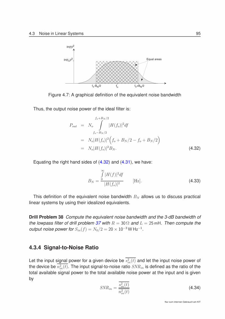
The integral is a constant for a given system frequency transfer function. We wouldlike to have a simple expression similar to (4.25) for the output noise power. A reason-able approach would be to define an equivalent noise bandwidth BN of an ideal filtersuch that the output noise power from the ideal filter and the real system are equal.As shown in Fig. 4.7, we assume that the ideal filters frequency transfer function is flatand equal to H(fo) within the bandwidth BN around the centre frequency fo and zerootherwise.


4.3 Noise in Linear Systems 95

fo-BN/2 fo+BN/2

|H(f)|2

|H(fo)|2 Equal areas

fo

Figure 4.7: A graphical definition of the equivalent noise bandwidth

Thus, the output noise power of the ideal filter is:

Pout = No

fo+BN/2!

fo−BN/2

|H(fo)|2df

= No|H(fo)|2%fo +BN/2− fo +BN/2

&

= No|H(fo)|2BN . (4.32)

Equating the right hand sides of (4.32) and (4.31), we have:

BN =

∞'

0

|H(f)|2df

|H(fo)|2[Hz]. (4.33)

This definition of the equivalent noise bandwidth BN allows us to discuss practicallinear systems by using their idealized equivalents.

Drill Problem 38 Compute the equivalent noise bandwidth and the 3-dB bandwidth ofthe lowpass filter of drill problem 37 with R = 30Ω and L = 25mH. Then compute theoutput noise power for Sin(f) = N0/2 = 20 × 10−3WHz−1.

4.3.4 Signal-to-Noise Ratio

Let the input signal power for a given device be s2in(t) and let the input noise power ofthe device be n2

in(t). The input signal-to-noise ratio SNRin is defined as the ratio of thetotal available signal power to the total available noise power at the input and is givenby

SNRin =s2in(t)

n2in(t)

(4.34)



Thus the SNR as defined above gives an indication of the amount of noise powerrelative to the signal power. Clearly the signal-to-noise ratio at the output of the deviceis analog to the above expression. Also the definition of the signal-to-noise ratio isindependent of the noise source and type.

The SNR is a power ratio which is most often expressed in Decibels:

SNRdB = 10 log 10(SNR) (4.35)

Thus an SNR = 13 dB means that the signal power is twenty times higher than thenoise power, while SNR = 0 dB means equal signal and noise power.

Drill Problem 39 An amplifier has an input SNR of 12 dB. Calculate the noise powerat the input if the signal power is −40 dBm.

Drill Problem 40 A signal 6 cos(2πft) V with f = 200Hz is fed to the input of the filterin drill problem 37. Taking the values of drill problem 38 compute the signal-to-noiseratio at output of the filter.

4.4 Naturally Occurring Noise

Natural radio noise in telecommunication systems is both picked up by the antenna aswell as generated within the system itself. The first effect can be accounted for by thecontribution which it makes to the antenna noise temperature. Attenuation due to watervapor and oxygen, clouds and precipitation is accompanied by thermal noise, lighteningand other atmospherics which further degrades the applicable signal-to-noise ratio. Inaddition, extraterrestrial noise of thermal or non-thermal origin may be picked up by thereceiving antenna.

This section gives an overview of the different types of naturally occurring noise anddefines appropriate quantities for modelling the effect of this noise. To start with, westate Planck’s radiation law, which is the the basis for other types of noise.

Planck’s Law

In 1900, Max Planck found the law that governs the emission of electromagnetic radi-ation from a black body in thermal equilibrium [Planck, 1900]. A black body is simplydefined as an idealized, perfectly opaque material that absorbs all the incident radia-tion at all frequencies, reflecting none. A body in thermodynamic equilibrium emits to


4.4 Naturally Occurring Noise 97

its environment the same amount of energy it absorbs from its environment. Hence, inaddition to being a perfect absorber, a blackbody also is a perfect emitter. The essentialpoint of Planck’s derivation is that energy can only be exchanged in discrete portionsor quanta equal to hf , where h is Planck’s constant h = 6.626 × 10−34 J s and f is thefrequency in Hertz.

Then, the energy of the ground level (or state) is 0, of the first level hf , of the secondlevel 2hf and so on. In general:

Ev = n · hf for v = 0, 1, 2 . . . (4.36)

where v is the level or state number. Given the number Nv of energy quanta (in Planck’spublications these are referred to as energy elements) occupying level v results in anenergy of vNvhf for that level. The total energy is obtained by summing up over allstates, thus

Etot = N0 · 0 +N1hf +N2 · 2hf +N3 · 3hf + . . . (4.37)

Now according to quantum mechanics, the probability of occupying an energy levelgoes down with e−∆E/kT where k = 1.38 × 10−23 J K−1 is the Boltzmann constant, T isthe absolute temperature in Kelvin, and ∆E the excess energy. Then, the number ofenergy quanta N1 at the first level is given by the number at ground state N0 multipliedby the probability e−hf/kT . Similarly N2 = N1e−hf/kT = N0e−2hf/kT and so on. The totalnumber of quanta is :

Ntot = N0

(1 + e−hf/kT + e−2hf/kT + e−3hf/kT + . . .

)(4.38)

To determine the average energy, we divide the total energy by the total number ofenergy quanta. The expression can be simplified to give:

E(f) =hf

ehf/kT − 1(4.39)

Using the density of modes we find Planck’s law for the black body radiation. Ex-pressed in terms of the brightness of the radiated energy from a blackbody this is givenby:

Bf(f) =2hf 3

c21

ehf/kT − 1(4.40)

4.4.1 Thermal Radiation

Thermal radiation is system inherent and is generated through the random thermalmotion of electrons in a conducting medium such as a resistor. The path of eachelectron is randomly oriented due to interaction with other electrons. The net effect



of the electron motion is a random current flowing in the conduction medium with anaverage value of zero. The power spectral density of thermal noise is given by Planck’sdistribution law (4.39). For the normal range of Temperatures and frequencies wellbelow the optical range the parameter hf/kT is very small, so that ehf/kT ≈ 1+hf/kT ,and (4.39) can be approximated by:

Sn(f) = kT (4.41)

The power spectral density as given by (4.41) is independent of frequency and henceis referred to as white noise spectrum. Within the bandwidth B the available noisepower then is

Pn = kTB (4.42)

The above expression shows, that if the bandwidth is fixed it is sufficient to know thetemperature in order to be able to compute the noise power. This is the reason, why itis common to speak of the noise temperature when referring to the noise power (evenif the noise source is not thermal).

For T =300K, i.e. at room temperature, we get a noise power of NT = −114 dBm perMHz bandwidth. It is worth remembering this number as a reference and using it tocompute the approximate noise power for a given bandwidth. For example the noisepower for a 20MHz system would be NT = −101 dBm.

Knowing the available power to the network, we want to define the cirucit equivalentof the noisy resistor. This is done by considering a voltage source of rms voltage Vn

connected in series with the resistor R.

Passivenetwork

PassivenetworkR Zin

R

ZinVn

Figure 4.8: Noisy resistor connected to a network (left) and its equivalent circuit (right)

The noise power delivered to a network of input impedance Zin is:

Pn =###

Vn

R + Zin

###2Rin (4.43)

where Rin is the resistive component of Zin. If Zin = R, which is the condition formaximum power transfer, we find that

Pn =V 2n

4R(4.44)



Substituting for Pn from (4.42) and solving for Vn gives

Vn ="

v2n(t) = 2√kTRB (4.45)

4.4.2 Extraterrestrial Noise

Space is the source of mostly broadband noise which can be considered as plane elec-tromagnetic waves. Cosmic radiation has to be accounted for if either the main lobe orthe sidelobes of the receiving antenna are directed towards space. The noise sourcesare both thermal and non-thermal emission from the Sun, the Moon, the Cassiopeiaand planets and from elsewhere in our galaxy and other galaxies.

If the emission is of thermal origin its contribution to noise power can be describedthrough the spectral brightness as given in (4.40) which is the power density in Wattper unit solid angle per unit area per Hertz. At radio-frequencies where hf ≪ kT thespectral brightness Bf is given by the Rayleigh-Jeans law:

Bf =2kTc

λ2in

*Watt

m2 · sr · Hertz

+(4.46)

whereTc is the brightness temperature,λ is the wavelength andk is Boltzmann’s constant

The actual noise power received within a narrow frequency range depends on thedirection of the main lobe and the side lobes of the receiving antenna and on theeffective area of the antenna. Thus in general the spectral brightness of an extendedsource is a function of the direction relative to the antenna coordinates. For discretesources (such as the Sun), which lie within the main lobe of the antenna and subtenda solid angle Ωs that is much smaller than the antenna main-beam solid angle, thespectral power density becomes

p =2kTc

λ2Ωs Wm−2 Hz (4.47)

Further use of the spectral brightness will be made in a later section when the totalnoise power percepted by an antenna will be evaluated in detail.

In the general case Bf varies as λn where n is known as the spectral index. Thus forthe thermal emission of a black body n = −2. For non-thermal emission (4.46) can stillbe used but the brightness temperature Tc is no longer related to the thermal emission



but is an equivalent brightness temperature, in addition the spectral index has to bespecified.

Background Radiation: The entire Universe is saturated with what is known asmicrowave background radiation, a remnant of the Big Bang. After the Big Bang, theformation of matter, space and time out of virtually nothing, the prevailing temperatureswere at first almost inconceivably high. However, as the Universe expanded the tem-perature sank to approximately −270 C, the temperature that it is today. The expansionof space lengthened the wavelength of the electromagnetic radiation until it entered themicrowave range. Today, this radiation can be measured reaching us evenly from alldirections of space, thus the term “background radiation”. It would “heat up” any colderobject to the space temperature of 3K (note that absolute zero Kelvin is −273 C)

Figure 4.9: Temperature of the cosmic microwave background radiation as determinedwith the COBE satellite during the first two years of observation. The planeof the Milky Way Galaxy is horizontal across the middle of each picture. Thetemperature range is 0 – 4K for the top, 3.3mK for the middle, and 18µK forthe bottom image respectively.



4.4.3 Absorption Noise

When energy is absorbed by a body the same energy is reradiated as noise as shownby the theory of black body emission. Otherwise the temperature of some bodies wouldrise and that of others fall. In the case of a radiating antenna the energy is partiallyabsorbed by the atmosphere and reradiated as noise. The effective absorption noisetemperature Tab given as a function of the ambient temperature Ta and the attenuationLa is:

Tab = Ta(La − 1) (4.48)

Note that Tab is not identical to the physical (ambient) temperature of the atmosphereand increases with increasing atmospheric attenuation. Table 4.1 shows some valuesfor La and Tab when the ambient temperature Ta is 300K.

La [dB] 0 1 3 10La (power ratio) 1 1.26 2 10Tab [K] 0 78 300 2700

Table 4.1: Absorption noise temperature Tab for different values of attenuation and anambient temperature Ta = 300K

The Attenuation of the atmosphere depends strongly on frequency. Water vapourand oxygen cause a high atmospheric attenuation in the 20GHz and 60GHz frequencybands. The frequency band below 10GHz exhibits the lowest noise temperature.

4.4.4 Additional Natural Noise Sources

Two additional types of noise should be mentioned here, these are:

Shot noise: this type of noise occurs when the quantisation of electrical charge carrierbecome manifest. It arises in physical devices when a charged particle movesthrough a potential gradient without collision and with a random starting time.This is the case in vacuum tubes due to the random emission of electrons fromthe cathode and in many semiconductor components as a result of the diffusionof minority carriers and the random generation and recombination of electron-hole pairs. For these cases the power spectral density is approximately flat up tofrequencies in the order of 1/τ , where τ is the transit time or lifetime of the chargecarriers. In terms of the mean current, the power spectral density is

Sshot = qi(t) + 2πi(t)2δ(f) (4.49)



where q is the charge of an electron = 1.6 · 10−19 coulomb. The first term in (4.49)corresponds to the ac or fluctuation part of the noise current and the second termcorresponds to the nonzero mean value.

1/f noise: lots of components exhibit 1/f noise which appears at low frequencies (de-pending on the process below 1MHz, 10kHz or 1kHz). There exist several the-ories about the origin of this noise which is difficult to measure due to the lowfrequency.


Bibliography

[Misra and Moreira, 1991] Misra, T. and Moreira, A. (1991). Simulation and perfor-mance evaluation of the real-time processor for the E-SAR system of DLR. Tech.note, German Aerospace Center, Microwaves and Radar Institute.

[Papoulis, 1984] Papoulis, A. (1984). Probability, random variables, and stochasticprocesses. McGraw-Hill, 2 edition.

[Planck, 1900] Planck, M. (1900). Zur Theorie des Gesetzes der Energieverteilungim Normalspectrum. contained in Verhandlungen der Deutschen PhysikalischenGesellschaft, (2, jahrgang 2):237–245.

[Proakis, 1989] Proakis, J. G. (1989). Digital Communications. McGraw-Hill, 2 edition.

[Stremler, 1982] Stremler, F. G. (1982). Introduction to Communication Systems.Addison-Wesley, 2 edition.

[Widrow et al., 1996] Widrow, B., Kollár, I., and Liu, M.-C. (1996). Statistical theory ofquantization. IEEE Transactions on Instrumentation and Measurement Magazine,45(2):353–361.

103

5 Noise Applications

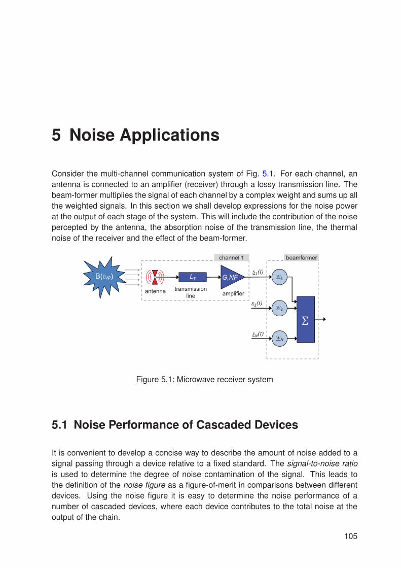
Consider the multi-channel communication system of Fig. 5.1. For each channel, anantenna is connected to an amplifier (receiver) through a lossy transmission line. Thebeam-former multiplies the signal of each channel by a complex weight and sums up allthe weighted signals. In this section we shall develop expressions for the noise powerat the output of each stage of the system. This will include the contribution of the noisepercepted by the antenna, the absorption noise of the transmission line, the thermalnoise of the receiver and the effect of the beam-former.

B(TM) LT

antenna

G,NFs1(t)

transmission line amplifier

w1

σw2

wN

s2(t)

sN(t)

beamformerchannel 1

Figure 5.1: Microwave receiver system

5.1 Noise Performance of Cascaded Devices

It is convenient to develop a concise way to describe the amount of noise added to asignal passing through a device relative to a fixed standard. The signal-to-noise ratiois used to determine the degree of noise contamination of the signal. This leads tothe definition of the noise figure as a figure-of-merit in comparisons between differentdevices. Using the noise figure it is easy to determine the noise performance of anumber of cascaded devices, where each device contributes to the total noise at theoutput of the chain.

105

106 5 Noise Applications

5.1.1 Noise Figure

Any real device always adds some noise so that the input signal-to-noise ratio is higherthan the output signal-to-noise ratio. To measure the amount of degradation, we definea noise figure, NF , to be the ratio between the input and output signal-to-noise ratios,respectively:

NF =SNRin

SNRout(5.1)

By definition, a fixed value for the input noise power is used when determining thenoise figure of a device using (5.1). This noise power is equivalent to the thermal noisepower provided by a resistor (as described in section 4.4.1) matched to the input andat a temperature of T0 = 290K.

The noise figure is commonly expressed in decibels:

NF dB = 10 log 10(NF ) (5.2)

The noise figure of a perfect noise free device is unity (or 0 dB), and the introductionof additional noise causes the noise figure to be larger than unity, i.e. NF dB > 0 dB.

A'

Nin+NeSin

NinG+NeGSinG

A

NinSin

NinG+NaddedSinG

Figure 5.2: Noisy two port device and its equivalent model

Consider the two port device A as shown in Fig. 5.2 with the transfer function H(f)and the equivalent noise bandwidth BN . The gain of the device, defined as the ratio ofthe signal output power to the signal input power, is G. Thus the output signal poweris1 Sout = SinG. The output noise power consists of the amplified input noise NinG inaddition to the noise added by the device itself Nadded, thus Nout = NinG + Nadded. Todescribe this added noise an equivalent noise free device A′ will be assumed with anoise generator at its input such that the total output noise of A and A′ are equal. Asshown in Fig. 5.2 the output noise becomes Nout = NinG +NeG and through (5.1) thenoise figure can be represented as

NF =SNRin

SNRout=

Sin/Nin

SinG/(NinG+NeG)= 1 +

Ne

Nin(5.3)

1for simplicity we will write Sout,in insted of PSout,in , and Nout,in instead of PNout,in . These quantitiesdenote the total power as described in section 4.2.4 equation (4.21)


5.1 Noise Performance of Cascaded Devices 107

The additional noise can be assumed to originate from an equivalent thermal noisesource at temperature Te thus Ne = kTeBN . By definition the input noise is Nin = kToBN

and substituting into (5.3) gives

NF = 1 +kTeBN

kToBN= 1 +

Te

To(5.4)

It should be noted that the effective temperature Te is only the equivalent physicaltemperature of a resistor that generates the same noise power as the device, the ac-tual noise source might not be thermal. Nevertheless (5.4) gives a simple formula tocalculate the effective temperature given the noise figure. The noise figure is useful forcomparing different systems regarding their noise performance. The noise tempera-ture on the other hand can be effectively used to calculate the actual amount of noisepresent in the system.

A better understanding of the meaning of the noise figure is possible by rewritingequation (5.3)

NF = 1 +Ne

Nin=

Nin +Ne

Nin=

G(Nin +Ne)

GNin=

Nout

GNin. (5.5)

From the above expression it is seen that the noise figure can be defined as the ratioof the total output noise to the total output noise of the noise free device, i.e.

NF =total output noise

total output noise of noise free device(5.6)

Note: At the first glance (5.4) and (5.5) seem to be frequency independent since thenoise figure is not dependent on the transfer function of the device. The justificationwould be that both noise and signal pass through the same device, so that |H(f)|cancels out when forming the signal-to-noise ratio. This however is not correct sincethe noise generated within the device Nadded will be frequency dependent in most cases,thus we should write Te(f) and keep in mind that F in (5.4) can at most be assumedconstant within some frequency range. Based on (5.5) we can write an expression forthe band noise figure NF which is frequency independent and gives the noise figurefor the total frequency band

NF =

∞'

0

F (f)|H(f)|2Nindf

∞'

0

|H(f)|2Nindf=

∞'

0

F (f)|H(f)|2df∞'

0

|H(f)|2df=

∞'

0

F (f)|H(f)|2df

BN |H(fo)|2(5.7)

In the above equation the gain G has been replaced by the square of the amplitudeof the transfer function |H(f)|2 which gives the relation between the input and outputspectral power density (see (4.28)). The total output noise at each frequency is foundas the product of the output noise from the noise free device |H(f)|2Nin times the noisefigure. The last term in (5.7) makes use of the equivalent bandwidth from section 4.3.3.



5.1.2 Noise Figure in Cascaded Systems

In this section expressions for the noise figure for a combination of cascaded networkswill be derived. Consider the cascaded two-port devices shown in Fig. 5.3.

A1 A2

Sin1Nin1+Ne1

Sout1=Sin1G1Nout1=Nin1G1+Ne1G1

Sin2Nin2+Ne2

Sout2=Sin2G2Nout2=Nin2G2+Ne2G2

Figure 5.3: Equivalent model for the transmission of noise through a cascaded system

Using the definition of the noise figure from (5.5) and knowing that the total noisepower output is Nout2 = G1G2(Nin +Ne1) + G2Ne2, the noise figure of the system NF12

will be:

NF 12 =total output noise

total output noise of noise free device=

G1G2(Nin +Ne1) +G2Ne2

NinG1G2(5.8)

The effective noise temperature of the cascaded system can readily be obtained fromNF 12 and (5.4).

Equations (5.8) can be generalised to a series of N cascaded networks [Bundy, 1998]:

NF 1N =G1G2 · · ·GN(Nin +Ne1) +G2 · · ·GNNe2 + · · ·+GN−1GnNeN−1 +GNNeN

NinG1G2 · · ·GN(5.9)

If the two-port networks are assumed to have identical input and output impedances,it can be shown that the minimum of the equivalent noise figure (or the equivalenttemperature) can be reached if the networks are arranged with increasing noise figuresof the individual stages.

The noise figure of cascaded networks (5.9) provides a simple and convenient wayto evaluate the noise performance of a system. An important point to note howeveris that the noise figure assumes a perfect match between the input and output of all


5.2 Microwave Receiver Noise Temperature 109

the networks and the cascaded structure. If this condition is not fullfiled, the easy-to-use equations can no longer be applied, the procedure is however straight forward andmainly involves the derivations already made.

Drill Problem 41 A receiver for satellite transmissions at 4GHz consists of an antennapreamplifier with a noise temperature of 127K and a gain of 20 dB. This is followed byan amplifier with a noise figure of 12 dB and a gain of 40 dB. Compute the overall noisefigure and equivalent noise temperature of the receiver. What would be the value of thenoise figure if the order of the amplifier and preamplifier would be exchanged? Assumethat the amplifiers are at a physical temperature of 290K.

5.2 Microwave Receiver Noise Temperature

Consider the system shown in Fig. 5.1. The voltage at the terminals of the input of thebeam-former is

x(t) = a(φ,ϑ)s(t) + n(t) (5.10)

where the first term represents the signal, while the second term is the noise voltage.Later the quantity of interest will be the power, which, assuming root-mean-squarevoltages, is written as

px = ⟨x(t)x∗(t)⟩ = |a(φ,ϑ)|2⟨|s(t)|2⟩+ ⟨|n(t)|2⟩ (5.11)

where ⟨·⟩ denotes time-domain averaging and ∗ the complex conjugate. In the aboveit has been assumed that the signal of interest is uncorrelated to the noise, thus⟨s(t)n∗(t)⟩ = 0, which is true for a non-multiplicative internal noise contribution.

In the following we investigate the various noise contributions, up to the input of thebeam-former.

5.2.1 Antenna Noise Temperature

The noise at the output terminals of a lossless antenna, c.f. Fig. ?? is considered. Allreal antennas are directional antennas [Balanis, 1997], which is the property of radi-ating or receiving electromagnetic waves more effectively in some directions than inothers. The directional properties of an antenna can be described through the radia-tion pattern (c.f. section 1.5). If we assume spherical coordinates, the radiation patternC(θ,ψ) gives the ratio of the field strength in a given direction (θ,ψ) from the antennato the maximum field strength. Whether we are dealing with a receiving or transmitting



antenna is indifferent for the definition of C(θ,ψ). Since the radiation pattern is normal-ized to the maximum value, the ratio of power density to maximum power density isgiven through C2(θ,ψ). When dealing with the received noise by the antenna, we willuse the radiation pattern as a weighting function to combine the effect of the differentnoise sources with the directional properties of the antenna.

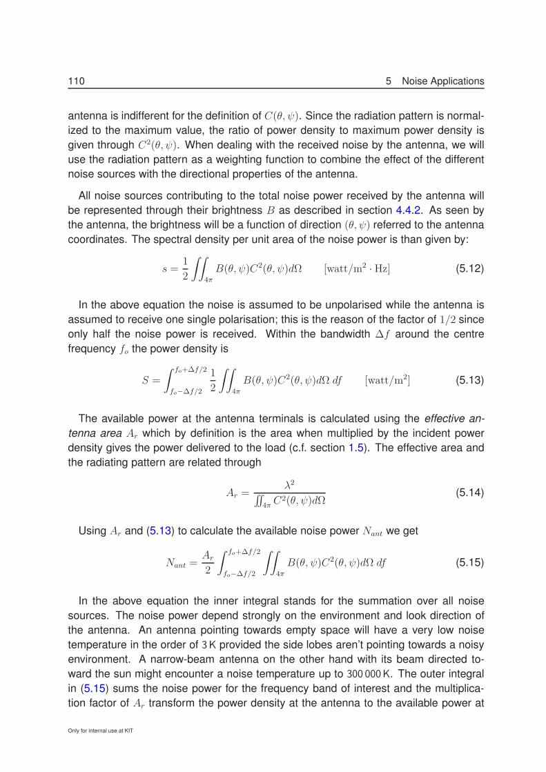
All noise sources contributing to the total noise power received by the antenna willbe represented through their brightness B as described in section 4.4.2. As seen bythe antenna, the brightness will be a function of direction (θ,ψ) referred to the antennacoordinates. The spectral density per unit area of the noise power is than given by:

s =1

2

!!

4π

B(θ,ψ)C2(θ,ψ)dΩ [watt/m2 · Hz] (5.12)

In the above equation the noise is assumed to be unpolarised while the antenna isassumed to receive one single polarisation; this is the reason of the factor of 1/2 sinceonly half the noise power is received. Within the bandwidth ∆f around the centrefrequency fo the power density is

S =

! fo+∆f/2

fo−∆f/2

1

2

!!

4π

B(θ,ψ)C2(θ,ψ)dΩ df [watt/m2] (5.13)

The available power at the antenna terminals is calculated using the effective an-tenna area Ar which by definition is the area when multiplied by the incident powerdensity gives the power delivered to the load (c.f. section 1.5). The effective area andthe radiating pattern are related through

Ar =λ2''

4π C2(θ,ψ)dΩ

(5.14)

Using Ar and (5.13) to calculate the available noise power Nant we get

Nant =Ar

2

! fo+∆f/2

fo−∆f/2

!!

4π

B(θ,ψ)C2(θ,ψ)dΩ df (5.15)

In the above equation the inner integral stands for the summation over all noisesources. The noise power depend strongly on the environment and look direction ofthe antenna. An antenna pointing towards empty space will have a very low noisetemperature in the order of 3K provided the side lobes aren’t pointing towards a noisyenvironment. A narrow-beam antenna on the other hand with its beam directed to-ward the sun might encounter a noise temperature up to 300 000K. The outer integralin (5.15) sums the noise power for the frequency band of interest and the multiplica-tion factor of Ar transform the power density at the antenna to the available power at



the antenna terminals, thus the effective area will also include the effect of antennamismatch.

An expression as given by (5.15) is not practical when dealing with or comparingdifferent receiving antennas. What is needed is a simple figure-of-merit such as theequivalent noise temperature of the antenna, which can be found by simplifying (5.15).A narrow bandwidth ∆f is assumed such that the spectral brightness (4.46) can con-sidered constant2 over ∆f . In addition, if the integration of the spectral brightnessis compared to the integration of the frequency transfer function as described in sec-tion 4.3.3, an equivalent bandwidth BN can be introduced which reduces the integra-tion over ∆f to the multiplication by the equivalent bandwidth at f0 = c/λ0, thus (5.15)becomes

Nant =Ar

2

! fo+∆f/2

fo−∆f/2

!!

4π

2kTc(θ,ψ)

λ2C2(θ,ψ)dΩ df (5.16)

=Ar

2

! f+∆f/2

f−∆f/2

2k

λ2

!!

4π

Tc(θ,ψ)C2(θ,ψ)dΩ df

= ArBNk

λ20

!!

4π

Tc(θ,ψ)C2(θ,ψ)dΩ

inserting (5.14) into the above equation gives

Nant = k

*''4π Tc(θ,ψ)C2(θ,ψ)dΩ''

4π C2(θ,ψ)dΩ

+BN (5.17)

Comparing the above equation with (4.42) for the thermal noise power from a resistorimmediately suggest the definition of an equivalent antenna noise temperature Tant ofthe form

Tant =

''4π Tc(θ,ψ)C2(θ,ψ)dΩ''

4π C2(θ,ψ)dΩ

(5.18)

If the antenna is replaced by a resistance Rr at temperature Tant, then according to(5.17) this resistance will generate the same noise power as by the antenna.

Consider a lossless microwave antenna placed inside an anechoic chamber main-tained at a constant temperature T as illustrated in Fig. 5.4. The absorbing chambercompletely encloses the antenna and is covered by absorbing materials which act asblackbody radiators. The power received by the antenna due to emission of the cham-ber is given by (5.17) with the brightness temperature Tc(θ,ψ) replaced by the constanttemperature T seen by the antenna. Solving the integral we get

Nant = k

*''4π TC

2(θ,ψ)dΩ''4π C

2(θ,ψ)dΩ

+BN = kTBN (5.19)

2note that the spectral brightness depends on frequency through 1/λ2 = f2/c2.



Antennaradiationpattern

Antenna

Absorber, T

Absorbing chamber

Nout = kTBNResistor

Rr Nout = kTBN⇔

Figure 5.4: Noise power of an antenna placed inside an absorbing chamber

which is the same power available from a resistor at temperature T as given in sec-tion 4.4.1. From the standpoint of an ideal receiver of bandwidth BN , the antennaconnected to its input terminals is equivalent to a resistance Rr known as the antennaradiation resistance. Although in both cases the receiver is connected to a “resistor”in the case of the real resistor the noise power available at its output terminal is deter-mined by the physical temperature of the resistor, while in the case of the antenna thepower available is determined by the temperature of the blackbody enclosure, whoswalls may be at any distance from the antenna. Moreover, the physical temperature ofthe antenna structure has no bearing on its output power as long as it is lossless.

An important perception from (5.19) is that the total noise power received by anantenna is independent of the radiation pattern of the antenna if the surrounding envi-ronment is assumed to have a constant brightness temperature.

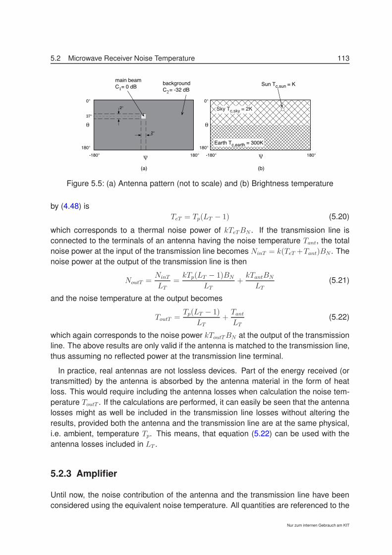
Drill Problem 42 A reflector antenna used for geostationary satellite receiving is po-sitioned such that its main beam lies at 37 above the horizon. For simplicity themain beam is supposed to extend over ± 1 both in elevation and azimuth as shownin Fig. 5.5(a). The value of the radiating pattern outside the main beam is −32 dB.As shown in Fig. 5.5(b), the antenna ’sees’ the sky with a brightness temperature ofTc,sky = 2K for θ < 90, the sun at Tc,sun = 8000K within a solid angle of Ωs = 0.5 andthe earth at Tc,earth = 300K for θ > 90. Calculate the antenna noise temperature withthe sun outside the main beam of the antenna.

5.2.2 Transmission Line

The noise temperature of a lossy transmission line can be calculated using the resultsof section 4.4.3. Consider the transmission line shown in Fig. 5.1. If the transmissionline is at the physical temperature Tp and has an attenuation of LT = 1/GT = Pin/Pout,then the equivalent noise temperature TeT at the input of the transmission line as given



-180° 180°

2°

2°

backgroundC2 = -32 dB

ψ -180° 180°ψ

Sun Tc,sun = K

Sky Tc,sky = 2K

Earth Tc,earth = 300K

0°

180°

θ

37°

(a) (b)

0°

180°

θ

main beamC1= 0 dB

Figure 5.5: (a) Antenna pattern (not to scale) and (b) Brightness temperature

by (4.48) isTeT = Tp(LT − 1) (5.20)

which corresponds to a thermal noise power of kTeTBN . If the transmission line isconnected to the terminals of an antenna having the noise temperature Tant, the totalnoise power at the input of the transmission line becomes NinT = k(TeT +Tant)BN . Thenoise power at the output of the transmission line is then

NoutT =NinT

LT=

kTp(LT − 1)BN

LT+

kTantBN

LT(5.21)

and the noise temperature at the output becomes

ToutT =Tp(LT − 1)

LT+

Tant

LT(5.22)

which again corresponds to the noise power kToutTBN at the output of the transmissionline. The above results are only valid if the antenna is matched to the transmission line,thus assuming no reflected power at the transmission line terminal.

In practice, real antennas are not lossless devices. Part of the energy received (ortransmitted) by the antenna is absorbed by the antenna material in the form of heatloss. This would require including the antenna losses when calculation the noise tem-perature ToutT . If the calculations are performed, it can easily be seen that the antennalosses might as well be included in the transmission line losses without altering theresults, provided both the antenna and the transmission line are at the same physical,i.e. ambient, temperature Tp. This means, that equation (5.22) can be used with theantenna losses included in LT .

5.2.3 Amplifier

Until now, the noise contribution of the antenna and the transmission line have beenconsidered using the equivalent noise temperature. All quantities are referenced to the



input of the amplifier, i.e. the noise power computed is at the input of the amplifier. Next,the aim is to get the noise power at the output of the amplifier, which is the noise powerthat goes into the beam-former. This is equal to the noise power kToutTBN amplified bythe gain of the G, and added to this we consider the contribution of the amplifier itselfas given by its noise figure NF . The total output noise power3 then becomes

⟨|n(t)|2⟩Ro

= k,TantG

LT+

Tp(LT − 1)G

LT+ T0(NF − 1)G

-BN (5.23)

where the connection to the noise term in (5.11) is made.

5.2.4 Beam-Forming

Next the beam-forming is considered. To account for the multiple input signals, we addthe index i where i = 1 . . . N and N is the total number of inputs (channels) to thebeam-former. Then (5.10) for channel i becomes

xi(t) = ai(φ,ϑ)s(t) + ni(t). (5.24)

Note that in the above equation, the signal s(t) is not indexed since it is the same to allinput channels; this is consistent with taking the electric field strength at the antennaaperture to be E(t) equally for all channels since it is attributed to a single point sourceat φ,ϑ.

Beamforming can then be described as the operation

y(t) =N$

i=1

wixi(t) (5.25)

where wi specify the (complex) unitless weights. Using vector notation, thus writingx = [x1(t), x2(t), . . . , xN (t)]T , this becomes:

y(t) = wTx = wTa(φ,ϑ)s(t) +wTn (5.26)

It should be pointed out, that the term wTa(φ,ϑ) in the above equation can be usedto explain the antenna array properties and effects; specifically, if normalized, this termrepresents the radiation pattern.

Now the power py at the output of the beam-former becomes

py = ⟨y(t)y∗(t)⟩ = ⟨(wTx)(wHx∗)⟩ (5.27)3A receiver described through its gain and noise figure could replace the amplifier, as such the descrip-

tion is rather general



Evaluating the above using (5.26) and simplifying yields:

py = wHa∗(φ,ϑ)aT (φ,ϑ)w⟨s(t)s∗(t)⟩+wH⟨u∗uT ⟩w (5.28)

where the earlier assumption that the signal and noise are uncorrelated is maintained.If the noise of the individual channels is taken to be uncorrelated then ⟨ni(t)n∗

j(t)⟩ = 0

for i = j and ⟨n∗nT ⟩ becomes a diagonal matrix.


Bibliography

[Balanis, 1997] Balanis, C. (1997). Antenna Theory Analysis & Design. John Wiley &Sons, 2 edition.

[Bundy, 1998] Bundy, S. C. (1998). Noise figure, antenna temperature and sensitivitylevel for wireless communication receivers. Microwave Journal, 41(3):108–116.

116

Documents

4NoiseinCommunicationSystems · 84 4 Noise in Communication Systems 4.2.1 Time-Averaged Noise Representations Informing averages of any signal, whether random or deterministic, weﬁndparameters