4K UHD – Sasken ProjectH.265CHETAN. MRICHA BARIYAR

Basics of compression

Multimedia compression Audio compression Image compression Video compression

Types of compression: Lossy compression

MP3, MP4, JPG Lossless compression

RAW, FLAC

Need for compression: Reduce memory footprint Fit for internet transmission across various devices

Basic Audio Compression

Audio compression works by reducing the accuracy of certain parts of a sound that are considered to be beyond the auditory resolution ability of most people. This method is commonly referred to as perceptual coding.

Variable Bit Rate (VBR) is made used. Dynamic range compression is applied at the source/sources itself.

Basic Image compression

Steps involved:1. If the color is represented in RGB mode, translate it toYCrCb.2. 2. Divide the file into 8 X 8 blocks.3. Transform the pixel information from the spatial domain to the frequency domain with the Discrete CosineTransform.4. Quantize the resulting values by dividing each coefficient by an integer value and rounding off to the nearest integer.5. Look at the resulting coefficients in a zigzag order. Do a run-length encoding of the coefficients ordered in this manner. Follow by Huffman coding.

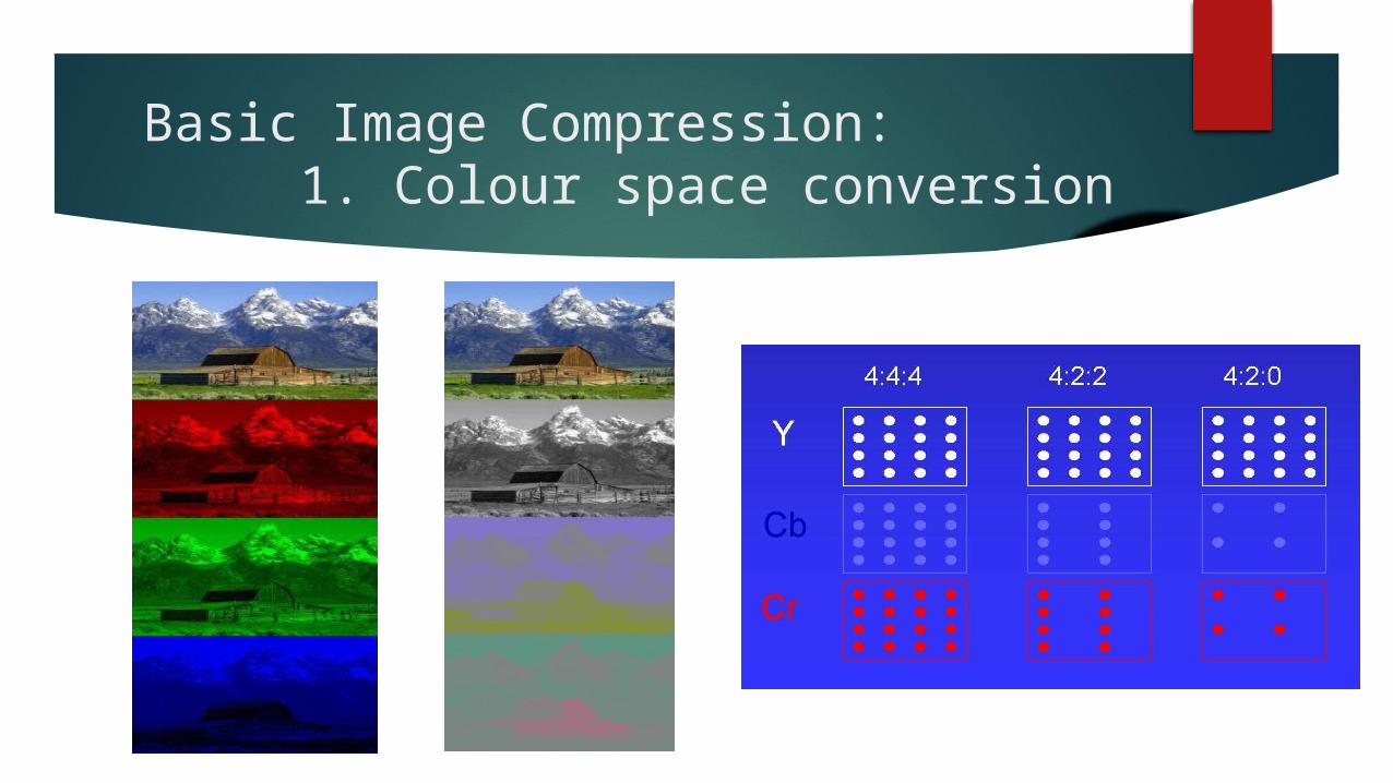
Basic Image Compression:1. Colour space

conversion

Basic Image Compression:2. Divide into 8 X 8

blocks With YCrCb color, we have 16 pixels of information in each block for the

Y component (though only 8 in each direction for the Cr and Cb components).

If the file doesn’t divide evenly into 8 X 8 blocks, extra pixels are added to the end and discarded after the compression.

Basic Image Compression:3. Discrete Cosine

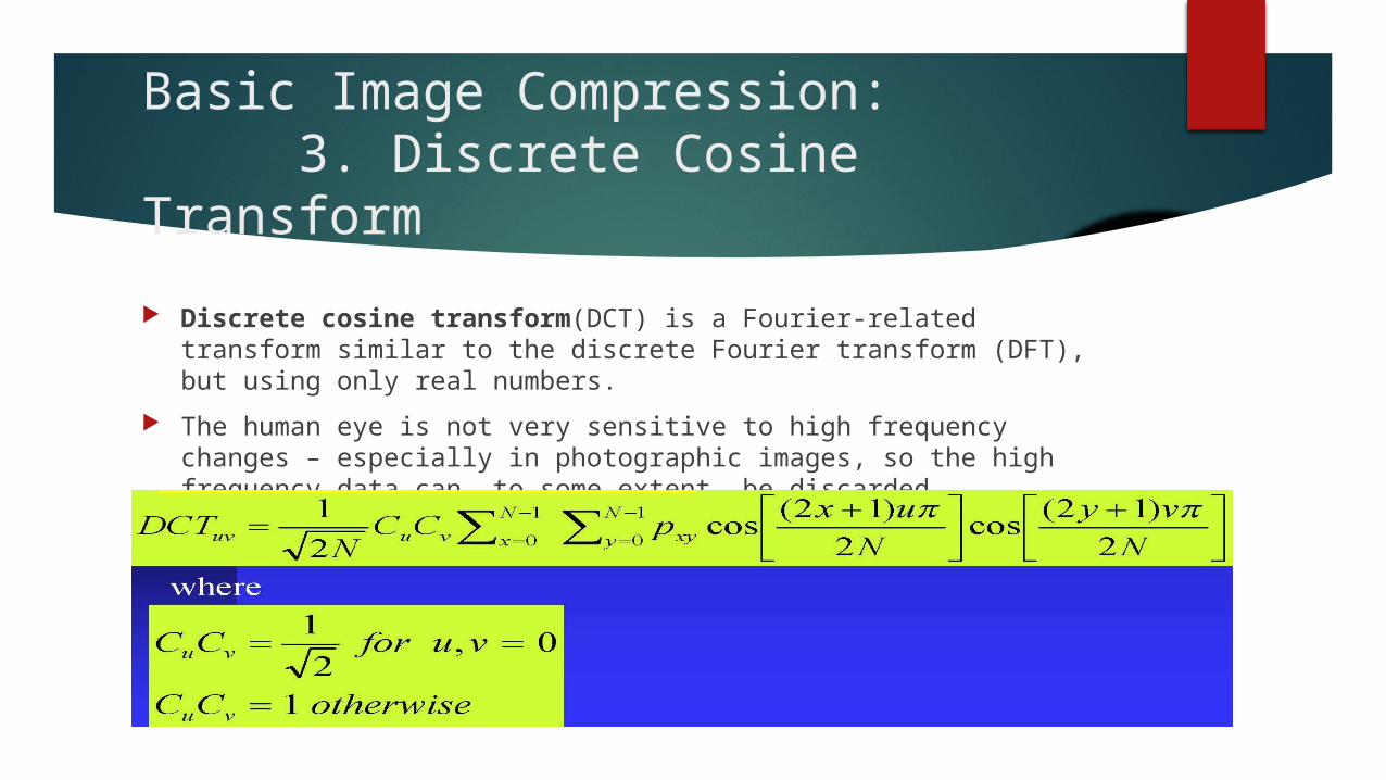
Transform Discrete cosine transform(DCT) is a Fourier-related transform similar

to the discrete Fourier transform (DFT), but using only real numbers. The human eye is not very sensitive to high frequency changes –

especially in photographic images, so the high frequency data can, to some extent, be discarded.

Basic Image Compression:4.

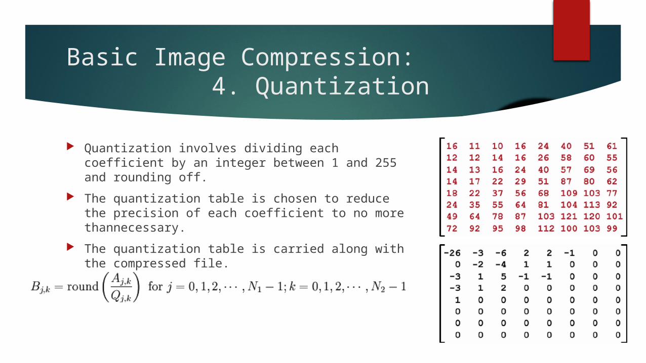
Quantization Quantization involves dividing each coefficient by

an integer between 1 and 255 and rounding off. The quantization table is chosen to reduce the

precision of each coefficient to no more thannecessary.

The quantization table is carried along with the compressed file.

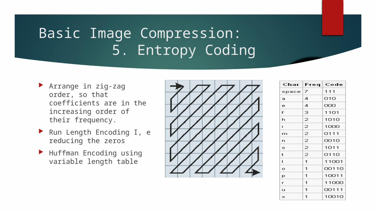
Basic Image Compression: 5. Entropy Coding

Arrange in zig-zag order, so that coefficients are in the increasing order of their frequency.

Run Length Encoding I, e reducing the zeros

Huffman Encoding using variable length table

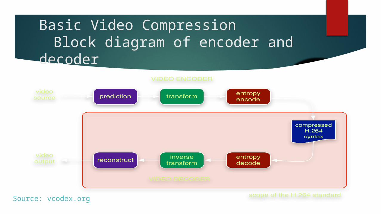
Basic Video CompressionBlock diagram of encoder and

decoder

Source: vcodex.org

Basic Video CompressionKey

words To encode a frame each operation is performed at macroblock (MB)

level Intra coded frame (I): every MB of the frame is coded using spatial

redundancy (as in image processing) Inter coded frame (P): most of the MBs of the frame are coded

exploiting temporal redundancy (in the past I,e using Motion Estimation and Motion Compensation)

Bi-predictive frame (B): most of the MBs of the frame are coded exploiting temporal redundancy in the past and in the future.

Group of Picture (GOP): sequence of pictures between two I-frames.

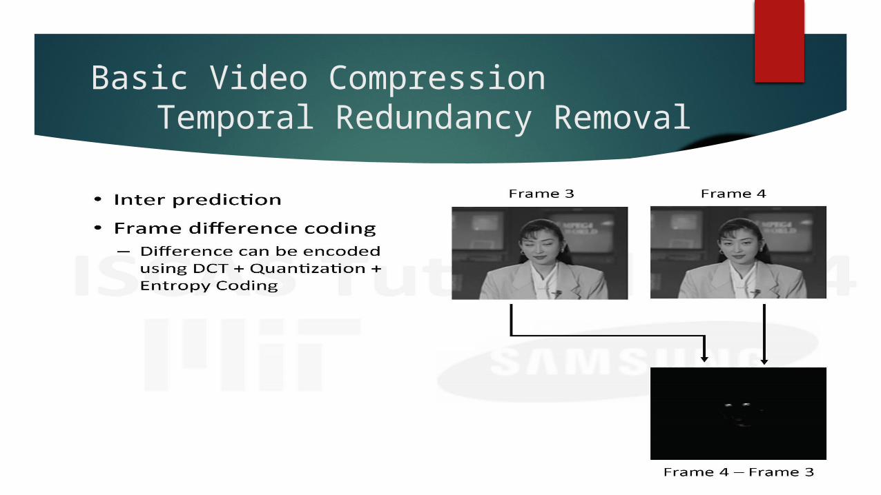
Basic Video CompressionTemporal Redundancy

Removal

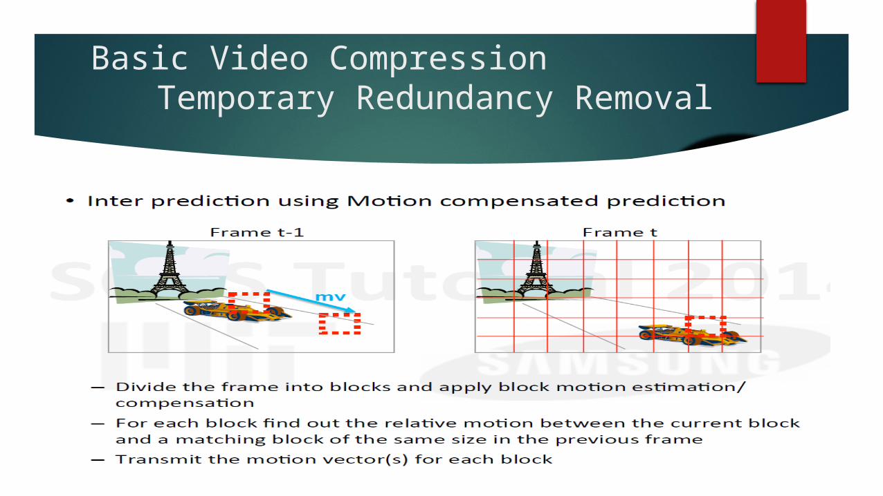
Basic Video CompressionTemporary Redundancy

Removal

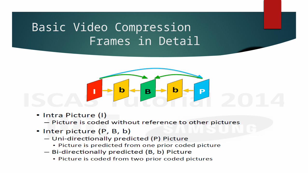
Basic Video CompressionFrames in Detail

Basic Video CompressionSummary of key steps in video

coding Intra prediction and Inter prediction Transform and quantization Entropy coding on syntax elements In loop filtering to reduce coding artifacts

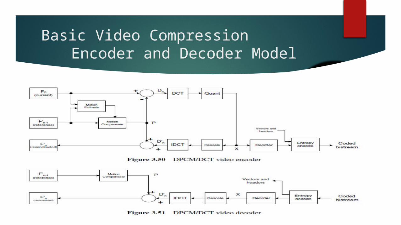
Basic Video CompressionEncoder and Decoder Model

High Efficiency Video Coding (HEVC)Feature Overview

2x compression compared to H.264/AVC High throughput (up to UHD 8K at 120fps) Low power support Built in parallelism and other implementation friendly features 3D and other multimedia support

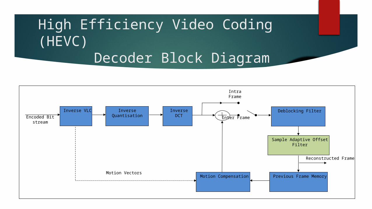
High Efficiency Video Coding (HEVC)Decoder Block

Diagram

Inverse VLC Inverse Quantisation Inverse DCT

Previous Frame MemoryMotion Compensation

Encoded Bit stream

Motion Vectors

Reconstructed Frame

Intra Frame

Inter FrameDeblocking Filter

Sample Adaptive Offset Filter

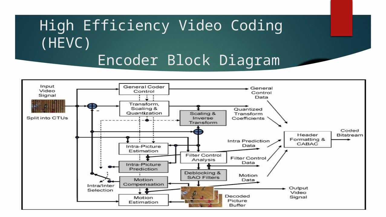
High Efficiency Video Coding (HEVC)Encoder Block

Diagram

High Efficiency Video Coding (HEVC)Coding Tools

Coding block size Intra Prediction Inter Prediction and Motion Compensation Inverse transforms Loop filtering Profiles, Tiers and Levels Parallel Processing Tools

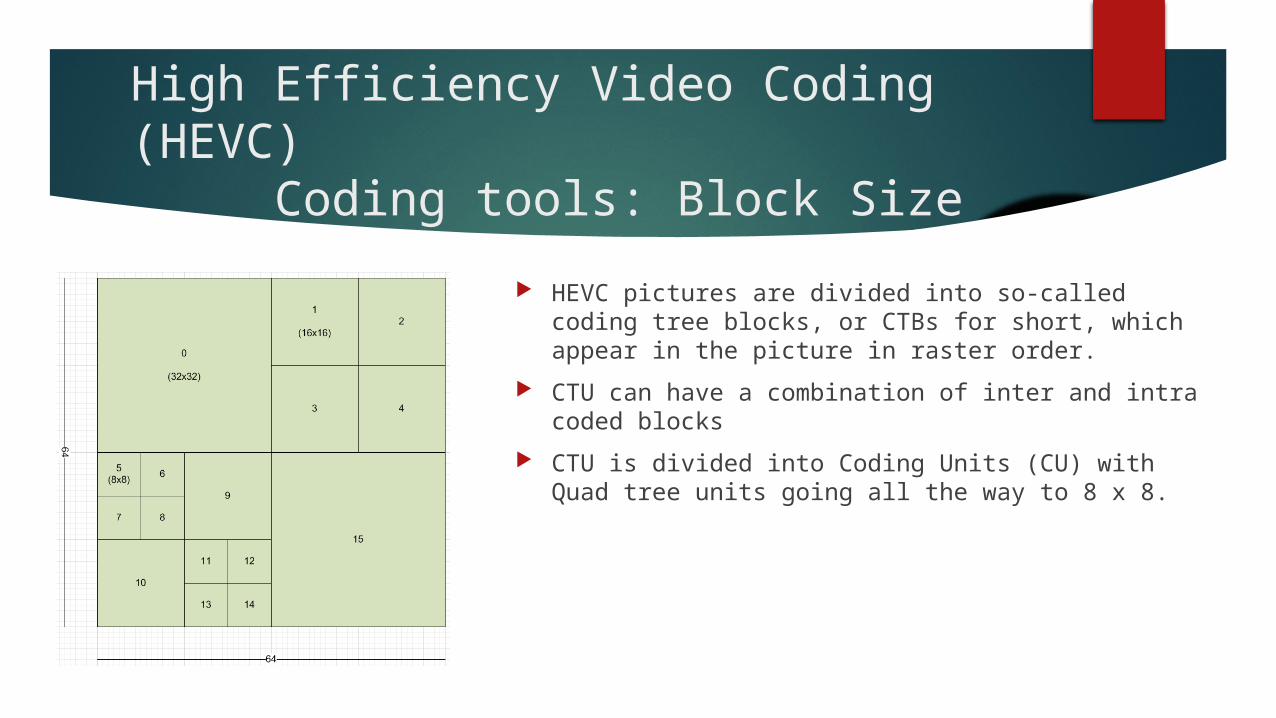
High Efficiency Video Coding (HEVC)Coding tools: Block Size

HEVC pictures are divided into so-called coding tree blocks, or CTBs for short, which appear in the picture in raster order.

CTU can have a combination of inter and intra coded blocks

CTU is divided into Coding Units (CU) with Quad tree units going all the way to 8 x 8.

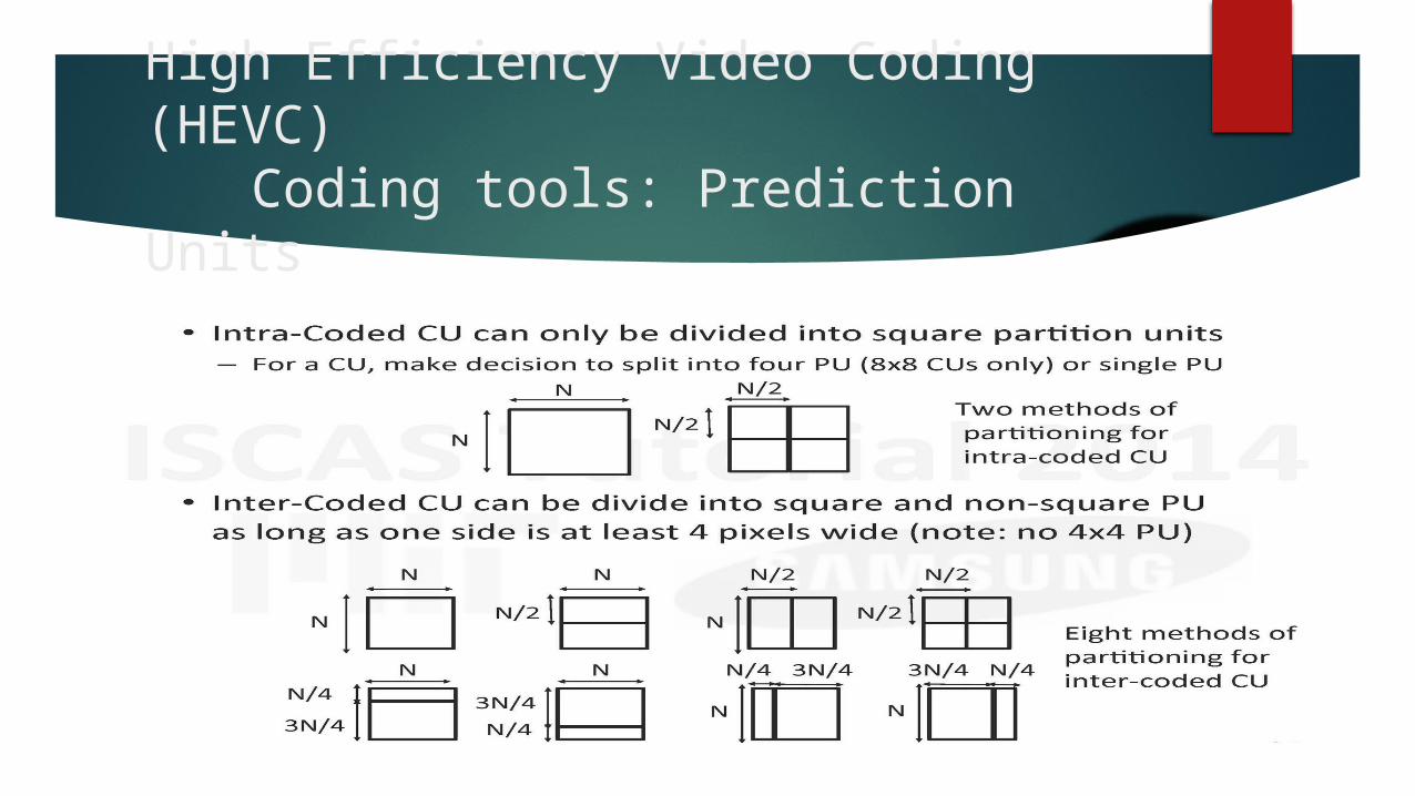
High Efficiency Video Coding (HEVC)Coding tools: Prediction Units

High Efficiency Video Coding (HEVC)Coding tools: Intra

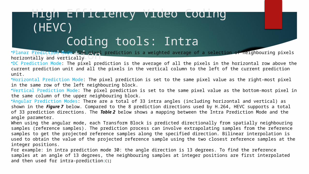
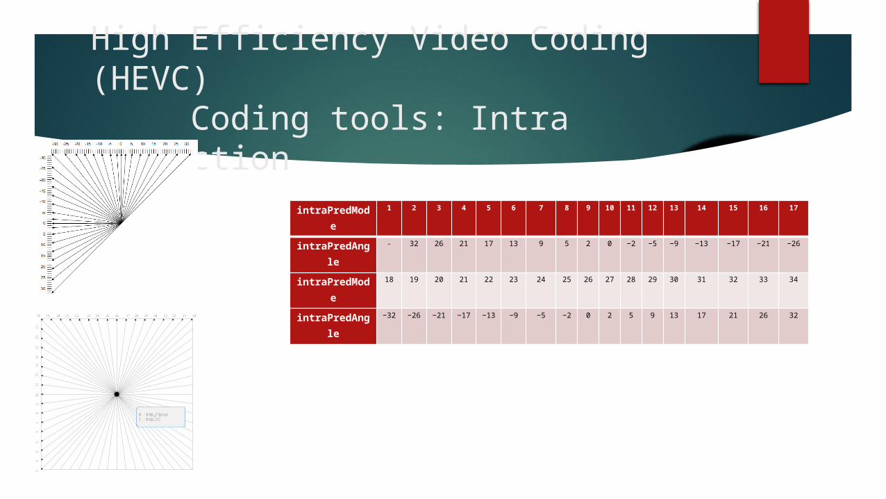
Prediction•Planar Prediction Mode: The pixel prediction is a weighted average of a selection of neighbouring pixels horizontally and vertically•DC Prediction Mode: The pixel prediction is the average of all the pixels in the horizontal row above the current prediction unit and all the pixels in the vertical column to the left of the current prediction unit.•Horizontal Prediction Mode: The pixel prediction is set to the same pixel value as the right-most pixel in the same row of the left neighbouring block.•Vertical Prediction Mode: The pixel prediction is set to the same pixel value as the bottom-most pixel in the same column of the upper neighbouring block.•Angular Prediction Modes: There are a total of 33 intra angles (including horizontal and vertical) as shown in the Figure 7 below. Compared to the 8 prediction directions used by H.264, HEVC supports a total of 33 prediction directions. The Table 2 below shows a mapping between the Intra Prediction Mode and the angle parameter. When using the angular mode, each Transform Block is predicted directionally from spatially neighbouring samples (reference samples). The prediction process can involve extrapolating samples from the reference samples to get the projected reference samples along the specified direction. Bilinear interpolation is used to obtain the value of the projected reference sample using the two closest reference samples at the integer positions. For example: in intra prediction mode 30: the angle direction is 13 degrees. To find the reference samples at an angle of 13 degrees, the neighbouring samples at integer positions are first interpolated and then used for intra-prediction [C1]

High Efficiency Video Coding (HEVC)Coding tools: Intra

Prediction

17 16 15 14 13 12 11 10 9 8 7 6 5 4 3 2

18 19 20 21 22 23 24 25 26 27 28 29 30 31 32 33 34

0 : Intra_Planar 1 : Intra_DC

intraPredMode

1 2 3 4 5 6 7 8 9 10 11 12 13 14 15 16 17

intraPredAngle

- 32 26 21 17 13 9 5 2 0 −2 −5 −9 −13 −17 −21 −26

intraPredMode

18 19 20 21 22 23 24 25 26 27 28 29 30 31 32 33 34

intraPredAngle

−32

−26

−21

−17

−13

−9 −5 −2 0 2 5 9 13 17 21 26 32

High Efficiency Video Coding (HEVC)Coding tools: Inter

PredictionLike AVC, HEVC has two reference lists: L0 and L1. They can hold 16 references each, but the maximum total number of unique pictures is 8. This means that to max out the lists you have to add the same picture more than once. The encoder may choose to do this to be able to predict off the same picture with different weights (weighted prediction).If you thought AVC had complex motion vector prediction, you haven’t seen anything yet. HEVC uses candidate list indexing. There are two MV prediction modes: Merge and AMVP (advanced motion vector prediction, although the spec doesn’t specifically call it that). The encoder decides between these two modes for each PU and signals it in the bitstream with a flag. Only the AMVP process can result in any desired MV, since it is the only one that codes an MV delta. Each mode builds a list of candidate MVs, and then selects one of them using an index coded in the bitstream. AMVP process: This process is performed once for each MV; so once per L0 or L1 PU, or twice for a bidirectional PU. The bitstream specifies the reference picture to use for each MV. A two-deep candidate list is formed: First, attempt to obtain the left predictor. Prefer A0 over A1, prefer the same list over the opposite list, and prefer a neighbor that point to the same picture over one that doesn’t. If no neighbor points to the same picture, scale the vector to match the picture distance (similar process as AVC temporal direct mode). If all this resulted in a valid candidate, add it to the candidate list. Next, attempt to obtain the upper predictor. Prefer B0 over B1, over B2, prefer a neighbor MV that points to the same picture over one that doesn’t. Neighbor scaling for the upper predictor is only done if it wasn’t done for the left neighbor, ensuring no more than one scaling operation per PU. Add the candidate to the list if one was found. If the list now still contains less than 2 candidates, find the temporal candidate (scaled MV according to picture distance), which is co-located with the right bottom of the PU. If that lies outside the CTB row, or outside the picture, or if the co-located PU is intra, try again with the center position. Add the temporal candidate to the list if one was found. If the candidate list is still empty, just add 0,0 vectors until full. Finally, with the transmitted index, select the right candidate and add in the transmitted MV delta.Phew, now merge mode: The merge process results in a candidate list of up to 5 entries deep, configured in the slice header. Each entry might end up being L0, L1 or bidirectional. First add at most 4 spatial candidates in this order: A1, B1, B0, A0, B2. A candidate cannot be added to the list if it is the same as one of the earlier candidates. Then, if the list still has room, add the temporal candidate, which is found by the same process as in AMVP. Then, if the list still has room, add bidirectional candidates formed by making combinations of the L0 and L1 vectors of the other candidates already in the list. Then finally if the list still isn’t full, add 0,0 MVs with increasing reference indices. The final motion is obtained by picking one of the up-to-5 candidates as signaled in the bitstream.Note that HEVC sub-samples the temporal motion vectors on a 16x16 grid. That means that a decoder only needs make room for two motion vectors (L0 and L1) per 16x16 region in the picture when it allocates the temporal motion vector buffer. When the decoder calculates the co-located position, it zeroes out the lower 4 bits of the x/y position, snapping the location to a multiple of 16. Regarding which picture is considered the co-located picture, that is signaled in the slice header. This picture must be the same for all slices in a picture, which is a great feature for hardware decoders since it enables the motion vectors to be queued up ahead of time without having to worry about slice boundaries.

High Efficiency Video Coding (HEVC)Coding tools: Inter

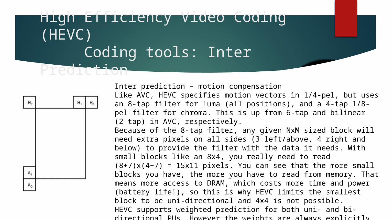
PredictionInter prediction – motion compensationLike AVC, HEVC specifies motion vectors in 1/4-pel, but uses an 8-tap filter for luma (all positions), and a 4-tap 1/8-pel filter for chroma. This is up from 6-tap and bilinear (2-tap) in AVC, respectively. Because of the 8-tap filter, any given NxM sized block will need extra pixels on all sides (3 left/above, 4 right and below) to provide the filter with the data it needs. With small blocks like an 8x4, you really need to read (8+7)x(4+7) = 15x11 pixels. You can see that the more small blocks you have, the more you have to read from memory. That means more access to DRAM, which costs more time and power (battery life!), so this is why HEVC limits the smallest block to be uni-directional and 4x4 is not possible.HEVC supports weighted prediction for both uni- and bi-directional PUs. However the weights are always explicitly transmitted in the slice header, there is no implicit weighted prediction like in AVC.

High Efficiency Video Coding (HEVC)Coding tools: Filtering and

deblocking Deblocking

Deblocking in HEVC is performed on the 8x8 grid only, unlike AVC which deblocks every 4x4 grid edge. All vertical edges in the picture are deblocked first, followed by all horizontal edges. The actual filter is very similar to AVC, but only boundary strengths 2, 1 and 0 are supported. Because of the 8-pixel separation between edges, edges do not depend on each other enabling a highly parallelized implementation. In theory you could perform the vertical edge filtering with one thread per 8-pixel column in the picture. Chroma is only deblocked when one of the PUs on either side of a particular edge is intra-coded.

SAOAfter deblocking is performed, a second filter optionally processes the picture. This filter is called Sample Adaptive Offset, or SAO. This relatively simple process is done on a per-CTB basis, and operates once on each pixel (so 64*64 + 32*32 + 32*32 = 6144 times in a 64x64 CTB). For each CTB, the bitstream codes a filter type and four offset values, which range from -7..7 (in 8-bit video). There are two types of filters: Band and Edge.Band Filter: Divide the sample range into 32 bands. A sample’s band is simply the upper 5 bits of its value. So samples with value 0..7 are in band 0, 8..15 in band 1 and so on. Then a band index is transmitted, along with the four offsets, that identifies four adjacent bands. So if the band index is 4, it means bands 4, 5, 6 and 7. If a pixel falls into one of these bands, add the corresponding offset to it.Edge Filter: Along with the four offsets, and edge mode is transmitted: 0-degree, 90-degree, 45-degree or 135-degree. Depending on the mode, two adjacent neighbor samples are picked from the 3x3 sample around the current sample. 90-degree means use the above and lower samples, 45-degree means upper-right and lower-left and so on. Each of these two neighbors can be less than, greater than or equal to the current sample. Depending on the outcome of these two comparisons, the sample is either unchanged or one of the four offsets is added to it.The offsets and filter modes are picked by the encoder in an attempt to make the CTB more closely match the source image. Often you will see in regions that have no motion or simple linear motion (like panning shots), the SAO filter will get turned off for inter pictures, since the “fixing” that the SAO filter did in the intra-picture carries forward through the inter pictures.

High Efficiency Video Coding (HEVC)Coding tools: Entropy Coding

HEVC performs entropy coding using CABAC only; there is no choice between CABAC and CAVLC like in AVC. Yay! The CABAC algorithm is nearly identical to AVC, but with a few minor improvements. There are about half as many context state variables as in AVC, and the initialization process is much simpler. In the design of the syntax (the sequence of values read from the bitstream), great care has been taken to group bypass-coded bins together as much as possible. CABAC decoding is inherently a very serial operation, making fast hardware implementations of CABAC difficult. However it is possible to decode more than one bypass bin at a time, and the bypass-bin grouping ensures hardware decoders can take advantage of this property.

High Efficiency Video Coding (HEVC)Coding tools: Parallel Processing

Tools Tiles: The picture is divided into a rectangular grid of CTBs, up to 20 columns and 22 rows. Each tile contains

an integer number of independently decodable CTBs. This means motion vector prediction and intra-prediction is not performed across tile boundaries, it is as if each tile is a separate picture. The only exception to this independence is that the two in-loop filters can filter across the tile boundaries. The slice header contains byte-offsets for each tile, so that multiple decoder threads can seek to the start of their respective tiles right away. A single-threaded decoder would simply process the tiles one by one in raster order. So how does this work with slices and slice segments? To avoid difficult situations, the HEVC spec says that if a tile contains multiple slices, the slices must not contain any CTBs outside that tile. Conversely, if a slice contains multiple tiles, the slice must start with the CTB at the beginning of the first tile and end with the CTB at the end of the last tile. These same rules apply to the dependent slice segments. The tile structure (size and number) can vary from picture to picture, allowing a smart multi-threaded encoder to load balance. 

Wavefront: Each CTB row can be decoded by its own thread. After a particular thread has completed the decoding of the second CTB in its row, the entropy decoder’s state is saved and transferred to the row below. Then the thread of the row below can start. This way there are no cross-thread prediction dependency issues. It does however require careful implementation to ensure a lower thread does not advance too far. Inter-thread communication is required.

High Efficiency Video Coding (HEVC)Coding tools: Profiles, Tiers and

Levels Each profile specifies a subset of algorithmic features and limits that shall be supported by all decoders conforming to that profile. Each

level specifies a set of limits on the values that may be taken by the syntax elements of the HEVC Specification. Level restrictions are established in terms of maximum sample rate, maximum picture size, maximum bit rate, minimum compression ratio

and capacities of the DPB, and the coded picture buffer (CPB) that holds compressed data prior to its decoding for data flow management purposes. Some applications have requirements that differ only in terms of maximum bit rate and CPB capacities and hence two tiers were specified for some levels — a Main Tier for most applications and a High Tier for use in the most demanding applications.

All profiles have the constraints of chroma subsampling limited to 4:2:0, the decoded picture buffer size is restricted to 6 pictures for the maximum luma picture size of a particular level and tiling is allowed, but optional. The profiles specified are:

Main Profile: This profile allows for a bit-depth of 8-bits per colour. Main 10 Profile: This profile allows for a bit-depth of 8–bits to 10-bits per colour. The higher bit-depth allows for a greater number of colours.

The Main 10 profile allows for improved video quality since it can support video with a higher bit depth than what is supported by the Main profile.

Main Still Picture Profile: The bit stream conforming to this profile shall contain only one picture. This profile allows for a single still picture to be encoded with the same constraints as the Main profile.

HEVC defines 2 tiers, Main Tier and High Tier. The High Tier allows a much higher bit rate than Main Tier at the same level. HEVC defines 13 levels: 1, 2, 2.1, 3, 3.1, 4, 4.1, 5, 5.1, 5.2, 6, 6.1, and 6.2. (For levels below level 4, only Main Tier is allowed, High Tier is

not allowed.)

THANK YOU