435 AUTOMATIC TARGET HAND-OFF USING CORRELATION … · JLocation of the target in the seeker FOV can best be accomplished using correlation techniques. The approach taken is to consider

U.LDEPARTMENT OF CMMERCE

AD-A036 435

AUTOMATIC TARGET HAND-OFF USING CORRELATION

TECHNIQUES

AUBURN UNIVERSITY

ALABAMA

31 JANUARY 1977

- -lz ' 6-.'

CID

:M.. A.t P -WAi.

'-'4-'---~g D W '"t

~- ~4- -Si

FZ1-:

'A>0 V,- G-0cv ,-

'"N ~JQr'',,6 IW4 r

Man~- QC.os=-Wzz~ -<.tW

- ~ ~ ~ ~ ~ ~ ~ ~ ~ ~ ~ ~ M W~> ~4-~:~' t ~--~~t--. -

-- 'it

-j ""MW W

A~%--'A'~~~4~>$g 2 - ~;4~t ~4- -""O

ri-.' all, - -

AIR ~ '--*--'4k'- -- r -

r. -~~r -s .- ',-o so---A . - V--

N-~~~ ~~ nun-y- Q- "W% ~ 'd52>A.-<- , -

K V~W AJ 41K ~ ~ ?V$~ts tAqn*R fAA3AN

VNP -Or\I AMY

-~j CA% AM M

;A _........... AUTOMATIC TARGET HAND-OFF USING

3U!CMTIi 1,a !a ,'Lf , e~CORRELATION TECHNIQUES

by

J. S. Boland, III, L. J. Pinson, G. R. Kane

M. A. Honnell, and E. G. Peters

Electrical Engineering DepartmentAuburn University.Auburn, Alabama 36830

Final Technical ReportFor the Period 5 December 1975 - 31 January 1977

This research work was supported byU.S. Amy Missile Command

Redstone Arsenal, Alabama 35809under Contract DAAHOl-76-C-O396

ENGINEERING EXPERIMENT STATIONAuburn University

Auburn, Alabama 36830

=D DDC

I'); IIII31 January 1977 1,AR 8 19 I

D

Cleared for Public Release; Distribution Unlimited

I,

SECUImTY CLASSIFICATION OF THIS PAGE iWm Dae eu

.. REPRT DOCUMENTATIOH PAGE EIRMIM IMmX1. REIONT NUMlel GOVT ACCESSION NO RECPIETS CATALOG NUMBER

14. TITLE (and &tItie) S. TYPE OF REPORT 6 PERIOD COVER9D

Final Technical Report,

AUTOMATIC TARGET HAND-OFF USING 5 Dec. 1975 - IJan. 9. 7CORRELATION TECHNIQUES .ERORMNG OR. R;OT MUMMR

7. AU T"OI(o) li. CONTRACT OR GRANT NMBIEtfse)

J. S. Boland, III, L. J. Pinson, G. R. Kane, OAAHO-76-C-0396M. A. Honne11, and E. G. Peters

S. PERFORMING ORGANIZATION NAME AND ADDRESS 10. PROGRAM ELEMENT PROJECT. TASK

AREA & WORK UNIT NUMBERS

Engineering Experiment StationAuburn UniversityAuburn, AL 36830

II. CONTROLLING OFFICE NAME AND ADDRESS 12. 1lEPORT DATE

Conmander, U.S. Army Missile Command 31 January 1977ATTN: DRSMI-RGC 12. NUMBER OF PAGES

Redstone Arsenal. AL 35809 / '014. MONITORING AGENCY NAME 4 ADDRESS(if diflerent fivm Controllin Office) IS. SECURITY CLASS. 1,0l thli report)

UNCLASSI FI ED'rte, DEC&ASSIFICATION/DOWNGRADING

SCHEDULE

IS, DISTRIBUTION STATEMENT (of ths Report)

Cleared for Public Release; Distribution Unlimited

17. DISTRIBUTION STATEMENT (of the abstract entered in Block 20, If different fhem Report)

IS. SUPPLEMENTARY NOTES

19. KEY WORDS (Continue on reverse side it necessary and Identify by block number)

Correlation, Target Hand-Off, Image Correlation

20. ABSTRACT (Continue an reverse d It necessary and idontiP- by blork nvmber)

,The problem of automatic haid-off of a target from a precision pointingand tracking system (FITS) to an imaging missile seeker is considered in thisreport. The approach taken is to search for the target in the seeke fieldof view (FOV) using the PTS video as a reference. When the target ' located,the seeker line of sight is adjusted automatically such that the target isat the center of its FOV at which point the seeker tracker can lock on to thetarget.

I o , 1473 EDITION OF I NOV S IS OSOLETE

SEC:URITY CLASSIFICATION OF THIS PAGE (1hen Dot Entered)

' *. JLocation of the target in the seeker FOV can best be accomplished usingcorrelation techniques. The approach taken is to consider the most accuratebut yet most costly in computation time and hardware requirements. Trade-offs are then considered in order to obtain a real-time correlator (i.e.,one which can compute the correlation surface at the rate of the incominglive video from the seeker). The effect of these trade-offs on correlationaccuracy and other system performance criteria is given. A correlationalgorithm is chosen and en implementation of this algorithm is given. Analternate implementation using an analog adder rather than a digital addertree is recommended.

I

TABLE OF CONTENTS

Page

LIST OF FIGURES ...... ......................... 3

LIST OF TABLES ..... .......................... 7

1. INTRODUCTION ........ ........................ 9

A. Scope of Work ............. . ........... 11B. Organization of Report ..... ................. 13

2. FORMULATION AND COMPARISON OF CORRELATION ALGORITHMS . . . . 15

A. Geometric Layout of PTS and MissileSeeker TV Images .................... 15

B. Image Comparison Methods ................ 18

Direct MethodFast Fourier Transform (FFT) MethodPhase Correlation MethodSequential Similarity Detection Algorithm (SSDA)

C. ... jyof Alage Comparison Methods ... .......... 23

image NormalizationProblems Associated with FFT and PhaseCorrelation Methods

Quantization of the Input Video SignalsImage Normalization Using the One-Bit QuantizerQuantization Effects on S/N Patio for theDirect and SSDA Correlation Methods

Implementation of the SSDA an' Direct MethodsUsing One-Bit Quantization

3. CORRELATION SYSTEM CONSIDERATIONS .................. 53

A. Deterrination of Sampling Frequency ............... 53B. Area Correlator ....... .................... 55C. Preprocessing of Input Video ..... .............. 57

High Resolution Image PreprocessingLow Resolution Image PreprocessingEffect of Quantization about Incorr-ect MeanPreprocessing for .iiffering Sensor Characteristics

1

TABLE OF CONTENTS (Con't)

D. Vibration Analysis ......... .. .. ....... 71E. Derivation of AX and AY Misalignment in LR Image .... ... 76F. Threshold Effects on Probability of False

Registration and Detection Probability .............. 79

False Alarm

Detection

G. Target Not in Seeker FOV ..... ................. 97

4. IMPLEMENTATION ....... ........................ 101

A. Implementation of One-Bit by One-Bit Real-TimeCorrelator. ........ 101

B. Block Diagram of'32 x 6Asrry Corre1ator Sstem... ,. 121

5. CONCLUSIONS Ap"n RECOt4ENDATIONS ..... ............... 131

A. Conclusions ..................... 131B. Objectives of a Technology'?rogram. ........ .... 133

REFERENCES ........... .. .. ... ........... 135

2

:-K-_

"itI

LIST OF FIGURES

Page

1. PTS equipment location on AH-l helicopter ............. 10

2. Target space projection of narrow and wide FOV images . . . 16

3. HR image projected onto LR image .... .............. 16

4. K x L HR image located at position (p,q) of N x M LR image . 17

5. Two functions to be correlated .... ............... 19

6. Quantizers ......... .. .. ... .. .. .. ... 29

7. Six level quantizer ...... ..................... 31

8. Layout for correlation of first line of two images ..... 31

9. Alternate one-bit quantizer ..................... 37

10. One-bit correlator input/output tables .............. 38

11. Outcomes of 19l121 ....... .......... .... 40

12. Comparison of the SSDA and Direct Double SummationMethods ......... .......................... 47

13. Reversed polarity one-bit quantizer. ................ 50

14. Tnput/output table for one-bit correlation ............ 51

15. Exclusive-OR implementation ................... 51

16. Preprocessing of HR image where W=3 .... ............ 58

17. Block diagram of preprocessor ..... ............... 58

18. Preprocessing where W = 3.25 ..... ................ 60

19. Method for pixel quantization .... ............... 65

20. Quantizers for the HR and LR images ................. 66

3

%I

LIST OF FIGURES (Con't)

Page

21. Effect of dc quantization le,el on the variancein the estimate of p .......................... 69

22. Image layout identifying p* and q* .................. 77

23. Image layout showing AX and AY ..... ................ 77

24. Quantized signal plus noise ..................... 81

25. Quantizer characteristics ....................... 81

26. Correlation technique ................. . .82

27. Detection and false alarm probabilities versusdecision threshold (KL=2048) .................... .88

28. Detection and false alarm probabilities versusdecision threshold (KL=1024) ..................... 89

29. Probability of detection versus probability offalse alarm; parameter dependence .... ............. 93

30. Effect of SNR and pixel rrismatch probability, c,on probability of a correct decision for eachpixel . . . . . . . . . . . . . . . . . . . . . . . . . . . . 95

31. Effect of different video SlR on probability ofmaking correct decision for each pixel .... ............ 96

32. Search patterns for missile seeker .................. 98

33. Block diagram of correlator hand-off system ........... 102

34. Logic for 12 x 1 correlator .... ................. 104

35. Extension of Figure 34 to produce a 12 x 16 correlator. . 105

36. Logic diagram for a 15 x 1 one-bit correlator .......... 107

37. Extension of Figure 36 to produce a 15 x 16 correlator. . .. 108

38. Items in pipe ....... ....................... 110

39. Correlator and adder tree ..... .................. Ill

40. Memory requirement for correlation computation .......... 115

4

LIST OF FIGURES (Can't)

Page

41. Method of computing mean video l',ve1 .. .. .. .. .. .... 115

42. Mean viden computation and quantizer .. .. .. .. .. .... 116

43. Circuit for computing the maximum (i.e., the registrationpoint). .. .. .. .. . .. .. .. .. ... .. . .... 118

44. Picture size (P x Q) with horizontal and vertical retP'aceR and S.. .. .. .. . .. .. ... .. .. .. .. .... 119

45. Retrace (Edge) effects on quantization .. .. .. .. .. ... 120

46. Binary noise source generator. .. .. . .. .. ...... 120

47. Averaging circuit for resolution reduction of HR video .. . 122

48. Blanking circuits for correlator during horikcontal andvertical retrace. .. .. .. .. . .. .. .. .. .. .... 123

49. Complete digit~l correlator circuit. .. .. .. .. ..... 125

5

$

LIST OF TABLES

Page

1. Results of S/N ratio analysis ................... 46

2. Horizontal and vertical resolution of 2.3 x 2.3

m~ter target ....... .. .. .. .. .. .. .. .. 56

3. Angular disturbances in s'eker LOS due to jitter ..... 75

4. Comparison of ECL vs. TTL logic correlators ... ........ 106

5. One-bit by one-bit correlator using ECL logic ......... 109

Precdhg page blink

1. INTRODUCTION

Currently the U. S. Army is developing a system for the acquisition,

tracking, and laser designation of military targets fro;n helicopters.

The Army is also developing terminal homing guided weapons capable of

destroying designated military targets. The Army is also beginning to

investigate missi.es which have imaging seekers rather than laser seekers

to provide guidance. This provides a true fire and forget weapor, ;ystem.

Very little attention has been given to-date to the problem of hand-off

of a target from the acquisition system to the imaging missile seeker.

This task can be accomplished by the gunner using the video displey from

both systems on his monitor. However, this technique is time consuming

resulting in increased helicopter exposure time. As a result the U. S.

Army Missile Command, Huntsville, Alabama let a contract with the

Engineering Experiment Station, Auburn University to study and make a

recommendation for a system to accomplish automatic hand-off of targets

from designators to imaging missile seekers using correlation techniques.

This report presents the result of that effort.

The overall system coisists of the helicopter with pilot and

gunner displays and controls, the pointing and tracking system (PTS),

either integrally mounted or on the stores wing of the helicopter as

shown in Figure 1, and the missiles located in a stores rack also

mounted on the wing of the helicopter. The helicopter supplies power

and other electronic support hardware for both systems. The pointing

9

sneding Pp blank

10

and tracking system typically consists of an optics train, line-of-sight

(LOS) stabilization system, day TV and forward looking infra-red (FLIR)

imaging systems, manual and autotrack system, laser range finder, and

associated electrcnics section. The imaging missile seeker could be

a day TV system or a FLIR. The current advanced television seeker

(ATVS) being tested by the Army [1) is composed of optical, day tele-

vision camera, TV tracker, mode control, stabilization .nd power supply

subsystems.

PILOTS INDICATOR GUNNER'S CONTROLRANGE AND GIMBAL CONSOLE; VIDEOANGLE DISPLAYS MONITOR, HAND

I'-. CONTROL, CONTROLS/INDICATORS

PTS PODELECTROMICS ANDTURRET ASSEMBLY

AMMUNITION BAYMOUNTED EQUIPMENT

Figure 1. PTS equipment location on AH-I helicopter.

11

In order to accomplish hand-off using correlation techniques,

the two signals being correlated must be similar. If both the PTS

and missile seeker are day TV systems sensitive in the same rela-

tive optical spectrum, correlation can be accomplished with very

little signal preprocessing. However, if the two signals are

dis4;miliar such as from a day TV and FLIR, then correlation Possibly

can be accomplished but only after considerable preprocessing of the

signals. For example, correlation on edges alone might work in this

case. The correlator developed in this report is for two day -

TV sensors. The problem of dissimilar sensors is discussed, however,

in Chapter III.

A. Scope of Work

The scope of work performed under this contract was tc analyze and

make recommendations on the hardware and software required to be used

in "handing-off" a target from a target acquisition device to an imaging

missile seeker. The function of an automatic correlator is to compare

the video signals from the hkgh resolution pointing and tracking system

(PTS) and from the missile seker and to generate error signals which

can be used to drive the missi'e seeker such that its aimpoint coincides

with that of the PTS. The scope of work as written in the contract

is given in the following six paragraphs for completeness.

The first phase will be to choose one or more candidate correlation

approaches. This will be done by surveying the literature for information

on existing correlation techniques. It is realized that some difficulty

12

may arise since most companies have developed correlation techniques

using their own funds and therefore consider them proprietarj. It

is likely, however, that some information on general correlation

techniques is available in the open literature.

Along with such information as is available on existing techniques,

an independent solution to the "hand-off" problem will be proposed

considering the variables involved (i.e., fields-of view, system

resolutions, stabilization, and others). The approach will be

to consider first the most accurate and complex correlation technique

and propose trade-offs in Phase Three.

Since the target may not necessarily be in the seeker field of

view (FOV), an algorithm will be proposed to slew the seeker TV until

the target is in its FOV. Of course, it is expected that this operation

will be very time consuming and should be avoided if possible. One

possible alternative is to determine and store in the fire control

computer boresight errors while in flight before a target is engaged.

The trade-off of additional software and computer memory required by

these two methods will be considered.

Phase Two, which will actually be conducted concurrently with

Phase One, will consist of an investigation of the hardware and software

needed for various combinations of PTS and missile seeker configurations.

Consideration will be given to differing fields-of-view, scan rates,

stabilization of TV cameras, boresight, and TV format (such as aspect

ratio, frames per second, etc.). The contractor will consider various

combinations and recommend the hardware and software necessary to

i;nplement each.

13

Phase Three will consist of the actual analysis of complexity

of the hardware/software necessary to Implement the various combinations

of Phase Two. This analysis will be presented in such a way that

MICOM will be able to use it to make a trade-off of the various

options available (e.g., complex/versatile vs. simple/closely bounded).

In Phase Four a correlation technique, along with the system

constraints, will be chosen in concert with the MICOM technical

director. This 6cision will be based on the results of the first

three phases. The hardware and software to implement this approach

will be completely specified, and the correlation algorithm will

be developed.

B. Organization of Report

All of the work outlined in the Scope of Work has been completed

and 1p documented in this final report. Chapter two formulates the

hand-off problem in greater detail and gives the various correlation

techniques considered. As expected, all companies contacted either

did not respond or gave very little detaii 'ntc their correlation

algorithms. As a result, the effort on this contract started with

a literature search of correlation techniques, defining the most

accurate but most time consuming methods, and making trade-offs in

order to arrive at an implementable solution.

Chapter three goes into detail on the many correlation system

considerations which had to be resolved before an implementable solution

could be attained. These considerations range from the system optics,

14TV sensor and TV forat, electronic preprocessing, sampling rates,

two system resolutions, vibration analysis, slaving of two systems

before correlation, derivation of error signals to drive the seeker

gimbals, and others.

Two possible implementations of the correlation algorithm are

given in Chapter four. The first implementation was considered to be

the state-of-the-art up until October when TRW publicly announed their

64 bit, 20 MHz bipolar correlator LSI circuit. The second implementation

incorporates this TRW chip and significantly simplifies the

hardware. The reason for giving both implementations is to emphasize

how LSI state-of-the-art can effect the real-time correlation problem.

It is known that TRW, and possibly other companies, is working on

another LSI correlator chip which will simplify the implementation

further or make possible an implementation which now is not feasible

for real-time correlation.

Chapter five gives the conclusions and recommendatioAs resulting

from the above work. Questions which arose during the course of this

work but were not answered due to lack of time or lack of simulation

facilitieJ are also given.

2. FORMULATION AND COMPARISON OF CORRELATION ALGORITHMS

In this chapter the basic correlation problem is formulated, four

methods are presented to solve the problem, and finally a comparison

of the four methods is given. Two of the methods are shown to be

impractical at the present state-of-the-art because of computational

burden.

A. Geometric Layout of PTS and Missile Seeker TV images

For the purpose of designing a correlator, this report will

consider hypothetical PTS and missile seeker day TV systems. To

design a correlator for a particular PTS and missile seeker, some of

the design parameters will have to be changed but the basic procedure

will be identical. Consider a PTS system with a vertical narrow field

of view (NFOV) of .50. a 525 line standard TV system with 2:1 interlace,

60 Hz field rate, or 30 Hz frame rate, and a 1:1 aspect ratio. The

sensor TV will be assumed to have a 20 vertical FOV with 4:3 aspect ratic,

a 525 line standard TV system with 2:1 interlace 60 Hz field rate,

or 30 Hz frame rate. Both systems because of verti:al retrace will

be considered to have 480 active TV lines.

One of the fundamental requirements for correlation using any of

the methods of the next section is that the two TV images be preprocessed

such that the scenes have the same spatial resolution. Since both TV

systems have 480 active TV line;, the PTS will have 4 times as many

lines on a given target as the rissile seeker TV because of the 1:4 FOV

ratio as shown in Figures 2 and 3. Since the resolution of the seeker15

16TV cannot bW increased, the obvious solution is to decrease the PTS

resolution by a factor of four. This can be accomplished by averaging

the PTS video as shown in Chapter 111. For the remainder of this chapter

it will be assumed that the PTS image, henceforth referred to as the

high resolution (HR) image, and the seeker image, henceforth referred

to as the la# resolution (LR) image have been preprocessed such that

they have the same spatial resolution prior to application of any

correlation algoritthm.

E]T48h Active

+Lines 480 Active Lines 4aHi gh Low

Resol ution ResolutionImage Image I(HR) (LR)

Figure 2. Target space projection of narrow & wf'e FOV images.

b b a

Figure 3. HR image projected onto LR image.

17

After the resolutions of the tw images are equalized a number of

correlation or' matching methods can be investigated. For the remainder

of this report the dimensional relationships between the two images

will be as shown in Figure 4.

p

N L

M.IFigure 4. K x L HR image located at position (p,q) of N x M LR image.

The missile seeker image is represented by a N X M array of points.

The values of N and M would be determied from a choice of sampling

rate and number of TV lines of the missile seeker system. The PTS image

or HR image is represented by a K X L array of points in Figure 4. This

K X L array might be all or only a portion, containing the target, of

the PTS image after its resolution has been changed to that of the missile

seeker image. The p and q dimensions in Figure 4 give the vertical and

horizontal position of the HR image in the LR image. These indices

start in the upper left corner of the LR image, where p = q = 0.

18

B. Image Comparison Methods

For digital matching of two images a number of alternatives

exist. In thtis section four candidate algorithms are presented and

explained. A detailed comparison of these methods is given in

Section C of this chapter.

1. Direct Method

The classical approach to the problem of determining where two

signals match is correlation. Consider two functions f (t) and: f2 (t) as shown in Figure 5. The correlation integral is defined to

be

C(T) -/ fl(t) f2(t + T)dt (1)

where T is allowed to take on values between -- and +'. The value of

T which nmaxiizes C(T) in Equation 1 is the correlation peak and is

defined to be the match point between the two signals. In Figure 5

this will occur when T = t2 - ti. It is obvious that determining the

correlation peak consists of multiplying one signal by the other signal

shifted by T and then evaluating the area under the resulting corve.

19

f1(t)

- t

t I

' 2 (t)

t2

Figure 5. Two functioris to be correlated.

If both signals are sampled and held, then Equation 1 can be

approximated by the following equation.

C(p) = T S fl(n)f2(n + p) (2)

where f(n) = f(nT) and f2(n + p) = f2(nT + pT) and T is the sampling

interval. As T becomes very small, the result in Equation 2 approaches

that of Equation 1 where the p which maximizes C(p) is defined as the

co,,relation point.

!IM

20

The two TV images arf first sampled and preprocessed to match

spatial resolution and then stored in arrays. The HR image is a K X L

array and the LR image ;s a N X N array as shown in Figure 4. Therefore

a two-dimensional discrete correlation algorithm is given by

R(pq) K I Hk(n,m) Lr(n+p,m+q)R~pq) 1 n-1 m'l

for 0 < p < N- K

0 _ q 1 M - L (3)

where R(p,q) is the correlation function, and the division by KL

is a scaling factor. Equation 3 is referred to as the Direct Method in

this report.

Using the algorithm of Equation 3, the selected K X L array of

HR points is compared to each array of LR points of dimension K X L

in the total N X M LR array. The algorithm produces the correlation

array R(p,q). In most situations the maximum value of the correlation

function indicates image registration or match. However, in tha

present case since the LR image spans a ider field-of-view, R(p,q)

is actually a cross-carrelation, and therefore it is possible that the

maximum value of the correlation functior, does not indicate a target

match between the HR and LR image. In orler that the maximum value

of the correlation function indicate targtt location in the LR image,

both image array values need to be normalized. Once normalization is

accomplished, the calculation of correlation points is insensitive to

magnitude values and depends on the pattern, of data points found in

the K X L arrays of the LR image. Therefore, in order to use the Direct

Method, image normalization must be implemented. Image normalization is

II21

discussed in further detail in Section C of this chapter.

2. Fast Fourier Transform (FFT) Method

Because of the transform relationship hetween correlation and

power spectral density, the cross correlation between the HR and LR

images is given by

R(p,q) = IFFT {IFFT rHR(n,m)] FFT [LR(n,m)))}

= IFFT {G(k,1)} (4)

where FFT [. ] is the fast fourier transform, IFFT is the inverse fast

fourier transform, G(k,l) is the cross power spectral density of HR

and LR and R(p,q) is the cross correlation function. In Equation 4

both the HR and LR arrays have to be the same size and preferably

be a power of two. To accomplish this both arrays are filled out with

zeroes to form 512 x 512 arrays. The result yields 512 x 512 values of

'i(p,q).

3. Phase Correlation Method

A major problem in correlating two different size images is that the

resultant correlation function is in fact a cross-correlation instead of

the desired auto-correlation. The auto-correlation function has its

maximum value for zero relative shift; this is not necessarily true for

the cross-correlation function. Thus it is quite possible that the

22cross-correlation function will have false peaks which are larger than

the peak for zero shift. The false peak condition can occur quite easily

for portions of the LR image of high brightness, especially if the

smller HR image is of lesser brightness. Therefore, the problem is

one which depends on relative magnitudes of the various sub-elements of

the larger image.

One technique that reduces magnitude effers in 4--, -ross-correlation

function is phase correlation. The phase correlation fnct'on between the

HR and LR images is given ty

R(pq) = IFFTI IFT[HR(n,m)) IFFT[LR(n,m]j (5)(IFFTLHR(nm)]) {FFT[LR(n,m)}I5

where * denotes the conjugate.

The phase correlation ma.thod is essentially a point-by-point

normalization in the frequency domain of the cross-power spectrum.

The same requirements on the size of the HR and LR arrays exists as

for the FFT method.

4. Sequential Similarity Detection Algorithm (SSDA)

Another algorithm for determining the similarity and amount of

registration between two images is known as a Sequential Similarity

Detection Algorithm (SSDA). Consider a K X L HR image (reference

image) and a N X M LR image. The SSDA registration surface is

cornputeu by adding the absolute value of the difference between the

HR and L pixels for each value of p and q as given by Equation 6.

k L 23E(p,q) =n J= IHR(nom) - LR (n+p, m+q)l (6)

for 0 1 p< N- K

0< q< M-L

The registration point (denoted by p*, q*) is the value of p and q for

which E is a minimum. The advantage of this method over the Direct

Method is that subtraction circuits rather than multiplication circuits

are needed for implementation. It should be pointed out, however, that

the SSDA method is not a correlation technique since Equation 6 is

not related to Equation 1, the correlation integral. A further co:parison

of these two methods is given in later sections of this report.

C. Analysis of Image Comparison Methods

1. Image Normalization

As stated in Section B of this chapter it is necessary to normalize

the correlation algorithms so that false peaks are less likely to occur.

False peaks can occur for the following reasons:

a. For correlation computations using the Fast Fourier Transform

(FFT), the two arrays must be the same size. To accomplish this the

HR array is filled in with zeroes to make it the same size as the LR

array (array sizes must be a power of two). Therefore the two images

being correlated are not identical which means the computation is a

cross-correlation rather than an auto-correlation. There is more of a

possibility for false peaks (any peak which does not correspond to

correct registration) in cross-correlation than in auto-correlation.

24

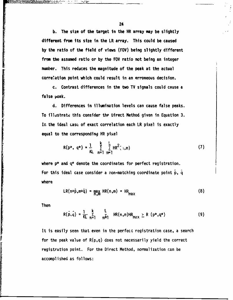
b. The size of the target in the HR array may be slightly

different from its size in the LR array. This could be caused

by the ratio of the field of views (FOV) being slightly different

from the assumed ratio or by the FOV ratio not being an integer

number. This reduces the magnitude of the peak at the actual

corre'ation point which could result in an erroneous decision.

c. Contrast differences in the two TV signals could cAuse a

false peak.

d. Differences in illumination levels can cause false peaks.

To illstrate this consider the Direct Method given in Equation 3.

In the ideal casL of exact correlation each LR pixel is exactly

equal to the corresponding HR pixel

k 2R(p*, q*) - 1 X HR 'Im) (7)

KL n=l m=l

where p* and q* denote the coordinates for perfect registration.

For this ideal case consider a non-matching coordinate point p,

whereLR(n+O,m+4) = wa HR(n,m) = HRmax (8)

Then" 1 k L

R(pq) = -L nl HR(nm)HRmax > R (p*,q*) (9)

It is easily seen that even in the perfect registration case, a search

for the peak value of R(p,q) does not necessarily yield the correct

registration point. For the Direct Method, normalization can be

accomplished as follows:

25

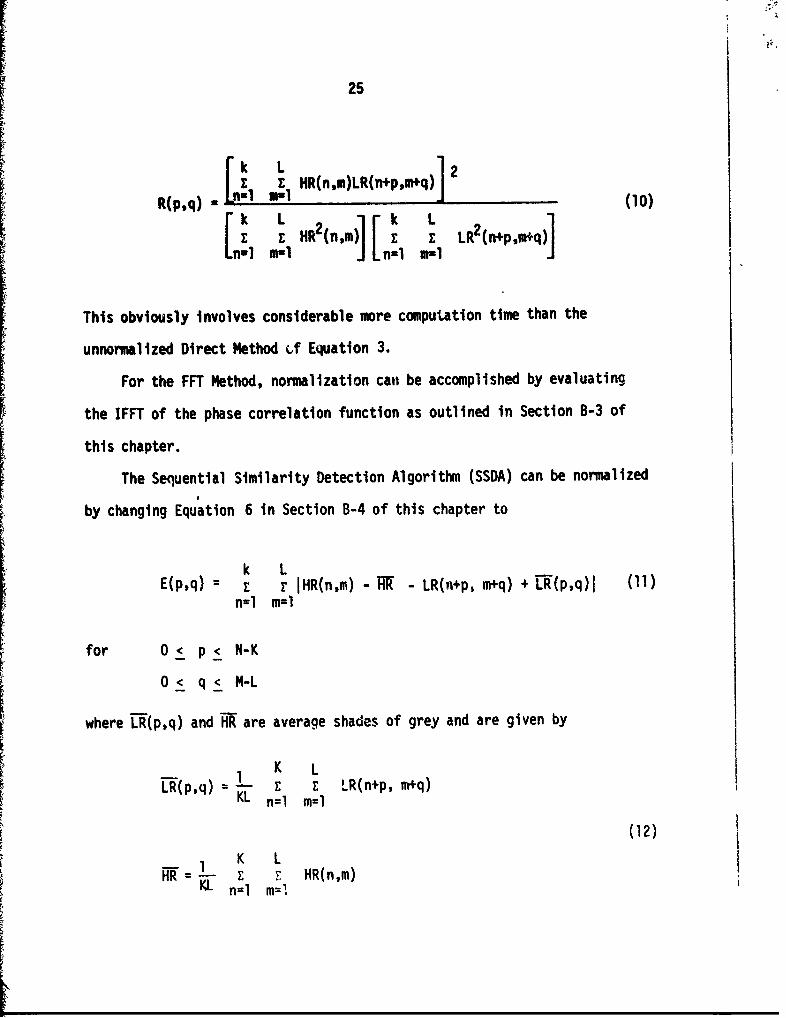
I E HR(n,m)LR(n+p,miq)]2

R(p,q) -1 M11 (10)

[i HR2(n,m [ LR2(n+p,nsqn1 Mail n-l m-1

This obviously involves considerable more computation time than the

unnormalized Direct Method Lf Equation 3.

For the FFT Method, normalization can be accomplished by evaluating

the IFFT of the phase correlation function as outlined in Section B-3 of

this chapter.

The Sequential Similarity Detection Algorithm (SSDA) can be normalized

by changing Equation 6 in Section B-4 of this chapter to

k LE(pq) = r " IHR(nm) - RR - LR(n+p, m+q) + -RE(p.q)I (11)

n=l m=l

for 0< p <_ N-K

0< q< M-L

where TR(p,q) and HR are average shades of grey and are given by

K L"R(p,q) - E Z LR(n+p, m+q)

KL n=1 m=1

(12)Ii1 K L

E R- HR(n,m)KL n=1 m=1

26

2. Problem Associated with FFT and Phase Correlation Methods

Of the four methods presented in Section B, the FFT and Phase

Correlation methods are the most difficult to implement. A number

of factors involved with these two methods make them somewhat less

than prime candidates for the hand-off problem. Both methods require

that the input arrays be square and that the dimension should be a

power of two. As shown in Section A, the HR image is preprocessed

because of its smaller FOV such that it is no longer the same

dimension as the LR array. Therefore it would be necessary to fill the

HR array with zeroes in order to make it the same size as the LR

array.

Since it is not known where the target may lie in the LR iffage,

it is required that the entire LR array be stored when using the

FFT or Phase Correlation methods. The HR image also has to be stored

in memory. Additional memory is also needed for the intermediate

steps of these methods. The Dirict Method and SSDA methods can be

used with only a small percentage of the memory needed for the FFT

and Phase Correlation methods. Also, both the FFT and Phase Correlation

algorithms involve, at orte step., complex multiplications of two-

diwiensional arrays. This argain would add greatly to the hardware needed

for their implementation that is not needed for the direct or SSDA methods.

Because of the increased amount of hardware required and the fdct that

the FFT and Phase Correlation methods cannot be inplemented in real time,

the FF and PhaseICorrelation methods were eliminated as canddate algorthms.

27

3. guantization of the Input Video Signals

All the algorithms discussed in Section B of this chapter require

that both the HR and LR video signals be digitized. The process of

digitizing continuous signals can be thought of as two separate steps.

The first is sampling at discrete instants of time and the second is

quantization. A discussion of the selectioni of an appropriate sampling

rate will be given in Chapters 3 and 4 of this',report. In this section

the different quantizers investigated are discussed and the trade-offs

used in choosing a particular quantizer are given.

The input-output relationship for the four basic quantizers con-

sidered in this section are shown in Figure 6. Figure 6 (a) is the

multibit quantizer or one that has a very large number of quantization

levels. Since there are many fairly inexpensive commercially available

8 bit A/D converters capable of operating at 10 MHz, they will be con-

sidered as multibit quantizers.

Figure 6 (b) gives the input-output rela tionship of a tw'o level

or one-bit quantizer. The weight of the output is +1 if the input is

above the mean voltage level and is -1 if the input is below the mean

voltage level. With this quantizer a means must be provided for

finding the average shade of grey of the K X L high resolution reference

image and of each of the K X L sub-arrays of the low resolution image

corresponding to each set of p and q values in Equation 3. This

could be done by quantizing the images with an 8 bit A/D ccnverter,

c mputing the average values in the host computer, during one frame,

and using these computed average values for one-bit quantization

during the following frame. The average signal level is not expected

to change significantly from frame-to-frame. If the average signal

level does change significantly from frame-to-frame, some form of

adaptive average computation should be employed. A sub-optimal but

real-time implementable solution to this problem is given in Chapter

3.

Figure 6 (c) is the Input-output relationship for a four level or

two-bit qcrantizer. Assuming the mean and standard deviation of the

input signal are known, there are two parameters, "a" and "vo/a", which

can be chosen so as to minimize the variance of the estimate of

R (.4., minimize the loss in S/N ratio due to quantization).

F'igure 6 (d) is the input-output relationship for a three level

quantiz.r. The advantage of this quantizer over the two-bit quantizer

is that the weiqhting of the products in Equation 3 are either + 1 or

0 which leads to a simpler circuit realization. The disadvantage is that

the liss in S/N ratio is greater than for the two-bit quantizer. The

mean and standard deviation (rms value) of the input video must be

calculated for this method.

The selection of the optimum parameters, a and V0/o, is made from

an analysis of the degradation, in the mean square S/N ratio. This

analysis is presented in Section C-5 of this chapter.

29

Output Output

Input Input

/ -1

a) Multibit quantizer b) One-bit quantizer

Output Output

aray f e it Input s

vor r a Input

t - o

c) Two-bit quantizer d) Three level quantizer

Figure 6. Quantizers

Nigher order quantizers are not considered since they would require

larger adders with larger computation times thereby leading to smller

arrays for real-time correlation. It will be shown in a later section

that the S/N ratio gain from using a larger reference array is greater

than the gain using higher-order logic in the quantizers in a smnaller

reference array.

30

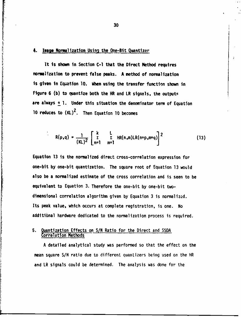
4. Luage Normalization Using the One-Bit Quanttzer

It is shown in Section C-1 that the Direct Method requires

normalization to prevent false peaks. A method of normalization

is given in Equation 10. When using the transfer function shown in

Figure 6 (b) to quantize both the HR and LR signals, the outputs

are always + 1. Under this situation the denominator term of Equation

10 reduces to (KL) Then Equation 10 becomes

IRFp q 1 12 )=~p~q E Z HR(n,m)LR(n+p,m+q) 2 (13)

2 n=l m=l

Equation 13 is the normalized direct cross-correlation expression for

one-bit by one-bit quantization. The square root of Equation 13 would

also be a normalized estimate of the cross correlation and is seen to be

equivalent to Equation 3. Therefore the one-bit by one-bit two-

dimensional correlation algorithm given by Equation 3 is normalized.

Its peak value, which occurs at complete registration, is one. No

additl6nal hardware dedicated to the normalization process is required.

5. quantization Effects on S/N Ratio for the Direct and SSDA

Correlation Methods

A detailed analytical study was performed so that the effect on the

mean square S/N ratio due to different quantizers being used on the HR

and LR signals could be determined. The analysis was done for the

- 1 31

quantizers shown in Figure 6 and also for the six level quantizer shown

in Figure 7.

Output

1/0 2/a InputI -1

-- a

Hlgure 7. Six level quantizer.

In this section the variance derivations for the Direct and SSDA methods

using one-bit quantization are presented. The results for the other quanti-

zers are summarized and a comparison of the two methods is presented.

a. Direct Method

Consider the estimation of the Direct Cross-Corr.lation function

for the first line of the high resolution image with the first line of

the low resolution image as shown in Figure 8. The estimation of the

[LR

Figure 8. Layout for correlation of first line of two images.

32

Direct Cross-Correlation function for the first line is given byL

R(l,q) - l 1 HR(l,m)LR(l, re+q) (14)

where HR and LR are the high resolution and low resolution images

respectively. To simpify the notation, the first row designation can

be dropped yielding

R(q) a 1 1 ()LRlm+l) (15)

If the sampling rate is less than or equal to the Nyquist rate, the

adjacent samples can be considered to be independent. Therefore,

except for the three or four values of q close to registration, the

correlation coefficient between the two images is small (i.e., p << 1).

If the two images are quantized with quantizers g, and g2 respectively,

then Equation 15 becomes

msl

The variance of this estimate is given by

2r = 2> >2 (17)R

where <R> denotes the expected value of R given by

<R> z E I M gIEHR(m)]g2[LR(m+q)] (18)m1j

I

33

However, because of the assuied independence of the samples, Equation

18 reduces to

1 gl[HR(m)J g2[LR(m+q) (19)

The first term in Equation 17 can be written as

1 LI<k2 I ng. l g[HR(m)]g92[LR(m+q)]gl [HR(n)]

•g2[LR(n+q)]" (20)

Separating the term for which n-- in Equation 20 yields

1 L-2> = I 1 [HR(m)]g 2 '.R(m+q)

+ L L ,/I

+L-T n 41 m ,l HRlm)]g2[LR(m+q)]gl[HR(n )]g2[LR(n+q)]/L I />

mn (21)

Consider the case where both quantizers g, and g2 have an input/

output relationship as shown in Figure 6(b), then Equation 19 becomes

0 0 Go OD<R> (1)f(HR,LR)d(HR)d(LR) +(

o/f(HR,LR)d(HR)d(LR) + f f (-1)f(HR,LR)d(HR)d(LR) +

(- R-d 000 0

f0 f (-I)f(HR,LR)d(:iR)d(LR) (22)

mm~~ C.w m

34

where f(HR,LR) is the jairit density function of the HR and LR images.

If f(HRLR) is symetric with zero mean, then Equation 22 reduces to

L<P> - l 1 [(1)(1/4) + (1)(1/4) + (-1)(1/4) + (-4)(1/4)]

or > (23)

Because of the assumed independence of the samples and the input/

output relationship of Figure 6(b), the first term in Equation 21 reduces

to

1 L11

and the second term in Equation 21 becomes

(L)(L-1) <g,[J>2 > (25)

Substituting Equations 23, 24, and 25 into Equation 17 yields

2 (26)R L

Equation 26 is an expression for the variance of the estimate

of R when the input is quantized into two levels. To obtain the

variance of the estimate of the true correlation of the two signals,

o 2, the relationship between R and p must be established. If the

input/output relationship for the quintized high resolution and

quantized low resolution video signals aie given by gl(HR) and g2(LR)

35

respectively, where g1 and g2 are both as shown in Figure 6(b), then

R(q) <I[HR]g2[LR(q)]> (27)

where the HR and LR(q) signals are Jointly normal with covariance p

given by

= KR LR(q) - KHR LR(cO> (28)

and correlation coefficient p given by

p H " R (29)

If X and Y are jointly normal random variables with covariance it

and the random variable Z is formed by Z - g(Xf, Y) where g(xy) is an

arbitrary function, then

E{Z} = E{g(X,Y)} " g(x,y)f(xy)dxdy (30)

where f(x,y) is the bivariate distribution function for the random

variables X and Y. Price's theorem [2], [3] states that

anE{g(xYY)} = E y)2nq("Y)

apn V-y

(31)

=Lff. " )x f(x,y)dxdyaxnay

n

36

Applying Price's theorem with n=l to the expression for R(q) in Equation

27 yields

=R~al- aE{gl[HRlg2[LR(q)]} E a2g1 HDR]g 2[LR(q)] (2

alla)= E aHR aLR(q)

and from Equation 29.

aR a R -= (33)

or

R HR aLR E { ) aLR(q))) (34)

However from Figure 6(b)

agl _ 26[HR] and a9g2_ 26[LR] (35)

and Equation 34 reduces to

-RrTTfq)i 26[HR]26r.LR] Ex{

I( HR2 _ 2pHRLR + LR2 d(HR)d(LR)2(1-o 2) 0HR LR 2 )]

r 2 (36)or ap~q -

a p T V 7

37

where it has been assumed that HR and LR are jointly gaussian. For the

case being considered p << 1 which leads to

! 1 ;. k 2 (37)pk T-

From Equation 37

k t (38)POne-Bit ROne-Bit

or 2 (39)

POne-Bit

using Equation 26.

If one uses the two level or one-bit quantizer with input/output

relationship as shcwn in Figure 9 and repeats the steps given above, one

finds the variance of this correlator to be

2 = 3 \) 1\ (40)

or a variance which is exactly three times that obtained using the one-

bit quantizer described by Figure 6(b). If the quantizer in Figure

6(b) quantizes to levels of ±n, repeating the steps above reveals that

the variance of the resulting correlator is again given by Equation 39.

iOutput

Input

Figure 9. Alternate one-bit quantizer.

rl im

38

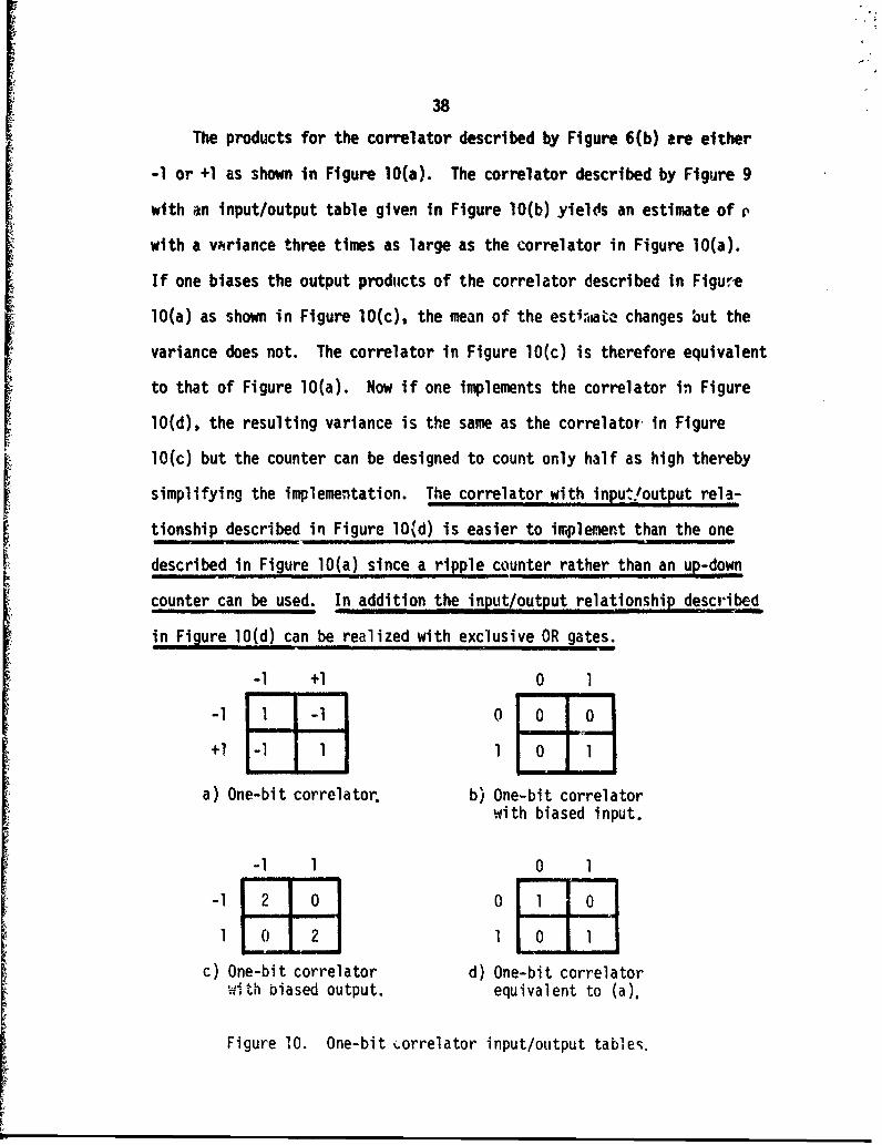
The products for the correlator described by Figure 6(b) are either

-1 or +1 as shown in Figure 10(a). The correlator described by Figure 9

with an input/output table given in Figure 10(b) yields an estimate of p

with a variance three times as large as the correlator in Figure 10(a).

If one biases the output products of the correlator described in Figure

10(a) as shown in Figure 10(c), the mean of the esti,.e changes but the

variance does not. The correlator in Figure 10(c) is therefore equivalent

to that of Figure 10(a). Now if one implements the correlator in Figure

10(d), the resulting variance is the same as the correlator in Figure

10(c) but the counter can be designed to count only half as high thereby

simplifying the implementation. The correlator with input!output rela-

tionship described in Figure 10(d) is easier to implement than the one

described in Figure 10(a) since a ripple counter rather than an up-down

counter can be used. In addition the input/output relationship described

in Figure 10(d) can be realized with exclusive OR gates.

-1 +1 0 1-1 1 -1 0 0 0

+1 -1 1 1 0 1

a) One-bit correlator b) One-bit correlatorwith biased input.

-Il 0

-1 2 0 1-1 2 0 0 1 0

1 0 2 1 0 1

c) One-bit correlator d) One-bit correlator

With biased output, equivalent to (a).

Figure 10. One-bit (.orrelator input/output tables.

39

b. SSDA Method

Consider the estimation of the SDA function for the first line of

the high reso'tition image with the first line of the low resolution

image as shown in Figure 8. The estimation equation for the SSDA

function is given by Equation 41 where HR and LR refer to high resolution

and low resolution images respectively.

L

R(L,q) - I 1HR(lm) - LR(l, m+q)i (41)

To simplify notation, the first row designation can be dropped, then

Equation 41 becomes

R(q) = i IHR(m) - LR(m+q)I (42)

Assume that the sampling rate is less than or equal to the Nyquist

rate. This means that adjacent samples are almost independent for all

values of q except for values near the point of registration. Therefore

for all cases, except the case near registration, the correlation

coefficient, p, is small and assumed to be much less than one.

If the two sampled lines of video are quantized with quantizers g,

arid g2 respectively, then Equation 42 is written as

R(q) 1 Jgl[HR(m)] - g2[LR(m+q)]l (43)m-l9

I] 40

TW-f~ m m64wir-wetbos can be investigated by

considering the cases of q for which the samples can be assumed inde-

pendent. The variance of the esttmamt, of R is given by

03 i(2> - (44)I. RAssume that the quantizing functions g, and g2 are given as in Figure 9.

Consider first <R>, given by Equation 45.

4> ~ g1(HR(m)J - 92[LR(m+q)JIl> (45)

Since the samples are independent, Equation 45 becomes

L<> . 1,/g1 [HR(m)] - g2 ELR(m+q)JI> (46)

Figurell shows the possible outcomes of the function Igl[HR(m)] - g2[LR(m+q)]I

for all combinations that the values g, and 92 can possess.

ql[HR(m)]

0 1

0 0 1g2[LR(m+q)]I1 0

Figure 11. Outcomes of 191 - g21,

Using the results of Figurel and expanding the expected value,

Equation 46 becomes

41

<i> L fof (1)f (HR,LRjk!(HR)d(LR)

(47)

saplsEqaton1+ 1 (I)f (HR%.LR)d(HR)d(LR)(

Assriing HR and LR to be jointly gaussian and assuming independent

samples, Equation 47 yields,

<i> = 1 2 fff ( HRLR)d(HR)dLR)

<R> C (L)(2) =48)

Therefore, the second term in Equation 44 is

<i> 1 z (49)

Next consider <V> given by Equation 50

<j2> < 17Zmi n= l jg1[HR(m)] - g2[LR(m+q)]Il

Igl[HR(n)] - g2[LR(n+q)]lI>

Separating terms for which m=n in Equation 50 yields

42

'i2, 1 .J ( KIg1Dft(M)] - 2[LR("4)]I21>L

1L L+ LL g[R~.) - [LR(fi'q)JI' (51)

mn

Ig1[HR(n)]- g2[LR(nq)I)>

Again using the results of Figure 1land the assumptions made previously,

Equation 51 becomes

I f (l)f(HR,LR)d(HR)d(LR) +,ul (-O 0

L L

+ J (1)f(HR,LR)d(HR)d(LR) + L I

0 mIfifl0 - m#n

IjO few (l)f(HRLR)d(HR)d(LR) + f Io (l)f(HRLR)d(HR)d(LR)[

-~ 0 0

f . j (1)f(HR,LR)d(HR)d(LR) + f *f (1)f (HR, LR) d(HR) d(LR)~

(52)

Equation 52 reduces to,

<2> 1 + (L-i) 1L+ (53)TL L4L 4(5)

43

Substituting Equations 49 and 53 into 44 yields

2 1 + 1- 1 Ia (54)

Of importance here is to find out how the mean square Signal-to-Noise

(M S/N) ratio is degraded by the use of different quantizers. .The

variance of the estimate of p, ap2, directly reflects the degradation.

The variance of p is found as follows.

Let

r(q) = E{1gl[HR(m)] - g2[LR(,,n)ji (55)

Assume that HR and LR have the joint gaussian density function given by

Equation 56

2 2[2(~P) HR2 2pHRLR + LR2

-- -- 7 OHR0LR GLRY2f(HR,LR) 1 2 -'aL(-p2" aHR (56)2HROLR(1p)

Then Equation 55 is written as

r(q): 1 ftigl[HR(m)], g2[LR(m+q)]l

21oHRLR(l p2) -.

(57)

E" ' ...Id(HR)d(LR)

2Using the results of Figurell and assuming p << 1, Equation 57 becomes

1 LO0 &[( 'HR"LR)lr(q) If JH L d(HR)d(LR)

2IHRCJLR or

+f-Jo 0 d(HR)d(LR)~ (58)

Using the expansion on ex for small ex -*i+X, Equation 58 becomes

r(q) = 20f r C2HR 2C 2 F +-I p(HR)(LR) 1d(HR)d(LR)(HR- o HR0LR

1 0 2H C2'LRr(q) wHo L C d(HRf] C d(LR) +

HR f(R (59

I Jo HR 2OHR d(HR)j LR C LR )(9-0 HR 0 cLR

Evaluating Equation 59 yields

45

r(q) I 2wo 2 I 2w hT.,0 LR . /

0

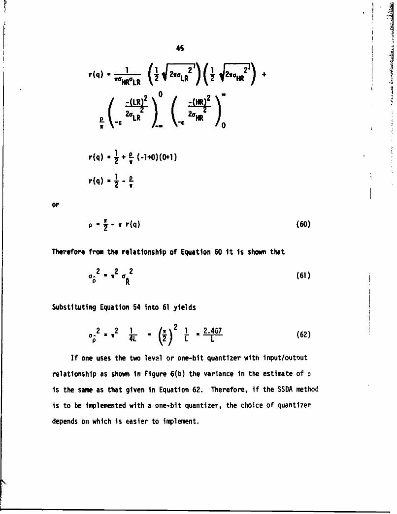
r(q) * + 2. (-1+O)(O+1)

or

p. " - w r(q) (60)

Therefore from the relationship of Equation 60 It is shown that

2 ., 2 (61)

0 f0

Substituting Equation 54 Into 61 yields

2 2 1 - ( 2 . 2.467(62

o- w -q (60)

If one uses the two leve.l or one-bit quantizer with input/outout

relationship as shown in Figure 6(b) the variance in the estimate of p

is the same as that given in Equation 62. Therefore, if the SSDA method

is to be implemented with a one-bit quantizer, the choice of quantizer

depends o, whtch is easier to implement.

46

c. Results of SIN Ratio Analysis for Higher Order Quantizers

The analysis of the degradation of the S/N ratio was extended for

both the Direct and SSDA methods to the cases where three, four, and six

level quantizers are used. As shown in Figures 6(c), 6(d), and 7, the

variables v0/,, v1/01 v2/0, a and b are chosen such that ap2 is minimized.

Table 1 shows the results of this analysis for both the SSDA and Direct

methods. The curves presented in Figure 12 show

Direct Method SSDA Method-I

No 2 Optimum 2 optimumQuantization F Parameters a ParametersLevels

2 2.467 ---- 2.467 1 ----__

3 1.525 v/o- 0.6 1.88 v/, .34 1.3 Vo/13 = . 1.715 V0o = 5

a=4 a=3

6 1.13 v1/a = 0.6 1.613 v!/a = .3

v2/a - 1.4 v2/a = .7

a=3 a=3

b=6 b=5

Table 1. Results of S/N ratio analysis.

a 2*L vs. no. of quantization levels for the two image matching methods

being considered. Figure 12 clearly shows that the Direct Method yields

a lower degradation in the ms S/N ratio for all quantizers except the

two level quantizer. Therefore, the conclusion can be made that the

SSDA method would notbe implemented using the higher order quantizers

if the decision were based only on degradation of the ms S/N ratio.

Ili F -

47

Hawver, since the SSOA method can be implemnted with less and faster

hardware than the Direct Method when more than tw levels are used, it

should not be ruled out as a candidate correlation alqorithm.2)

V 2 x L 0- Direct Method

2.46 A - SSDA Method

2

23 4 5 6

No. of Quantization Levels

Figure 12. Comparison of the SSDA and Direct Double Summation Methods

From Table 1 and Figure 12 one can draw some conclusions about

correlator design parameters (eg., reference array size, number of

quantization levels, and statistical accuracy). From Table 1 the

degradation in the mean square S/N ratio for both methods using any

number of quantization levels is inversely proportional to the number

of pixels used in the reference array (i.e., doubling the number of

pixels in the reference array halves the S/N ratio degradation for a

given number of quantization levels). Also from Figure 12 the degra-

dation in the S/N ratio can be improved by increasing the number of

quantization levels. However, relatively little improvement is gained

by using more than four levels (2-bits) with either the Direct or SSDA

48

method while the hardare to implement more than four levels increases

significantly. The conclusion is that a correlator using either the

Direct or SSDA method should have the video pixels quantized to two,

three, or four levels.

If the correlator is to operate in real time, then the sampling

period of the incoming live video dictates the amount of time available

for each correlation :omputation. However, increasing the size of the

reference array and increasing the number of quantization levels (eg.,

from two to four levels) both require more hardware and a longer compu-

tation time. From Table 1 increasing the number of quantization levels

from two to four increases the ms S/N ratio by 2.467/1.3 or 1.898 for

the Direct Method and by 2.467/1.715 or 1.438 for the SSDA method. The

computations, however, using four levels require more time. In fact from

data books on present state-of-the-art hardware one could more than

double the size of the reference array with this increased computation

time using two level quantization. This increase in the size of the

reference array would more than double the ms S/N ratio. Therefore, the

trade-off is to make the reference array size as large as possible for

real-time computation. Because of hardware considerations it is usually

desirable to make each reference array dimension a power of two (i.e.,

16x16, 32x32, 32x64, 64x64, etc.). If for example a 32x32 reference

array in a two level correlator can be computed in real time but a

32x64 reference array can not, then one might consider using three or

four levels in this 32x32 correlator if time would allow. In other

49

words the trade-off is to use as large a reference array as possible,

then consider usinq more than two levels if time permits.

One additional consideration when going from two level to three or

four level quantization should be pointed out. When quantizing to two

levels, each KxL subarray of the LR video should be quantized to one

level when above the mean and to the other level when below the mean of

that KxL subarray. For each value of p and q in Equation 3 or 6 all of

the KxL pixels in that subarray should be quantized about the mean of

that subarray. Quantizing about some moving average mean or about the

mean of the entire NxM LR image leads to errors in the correlation

computation. However, since it is not practical to do this, some trade-

off technique is usually devised. If a three or four level quantizer

is used,then the standard deviation as well as the mean of each KxL

subarray should be comptited. To use any other technique to find vo /a

in Table I leads to errors in the correlation computation. In fact

these additional errors could be larger than the gain in going from a

two level to a three or four level quantizer. The amount of error

induced by inaccurate values of mean and standard deviation in the

quantization is scene dependent. The conclusion is that if one uses a

three or four level quantizer, care should be taken in the computation

of the mean and standard deviation in order to prevent a significant

loss in the S/N ratio due to inaccuracies in these computations.

6. Implementation of the SSDA and D,'iect Methods Using One-Bit

Quantization

iaen both the HR and LR video are quantized to two levels, then

from Table 1 the Direct and SSDA methods have the same ms S/N ratio.

50

In this section the it)lementation of the two methods using exclusive

OR gates is shown to be equivalent. The conclusion is that when

quantizing to tbo levels, the SSDA and Direct methods are equivalent.

This is not the case when one or both video signals are qUantize;d to

more than two levels. In this case the SSDA method is not; a true

correlation technique while the Direct method is.

a. Direct Method

Consider first that the HR and LR video have zero mean and that

the HR video i; quantized by the input/output relationship shown in

Figure 9. Then if the LR video is quantized by the input/output

relationship shown in Figure 13, the correlator inputs when the input

video match are given by 01 and 10 and video mismatch are given by 00

and 11 input combinations. If the output of the correlator ir to be

1 when the input video match and 0 when the input video mismatch, then

the input/output table is given in Figure 14 and can be implemented

using an exclusive OR (0J) gate as shown in Figure 15. Implementation

of the entire array is given in Chapter 4. Using this method, the peak

value corresponds to registration of the two images.

LRq

1

LR

Figure 13. Reversed polarity one-bit quantizer.

51

q 0 1

1 1 0

Figure 14. Input/output table for one-bit correlation.

L Correlation

value

Figure 15. Exclusive-OR implementation.

b. SSDA

The SSDA implementation is similar to that given above, however the

quantizer given in Figure 9 is used to quantize both signals. The out-

cone of the SSDA algorithm is shown in Figure 11. The states 00 and 11

now represent matched samples and 01 and 10 represent mismatch. The

circuit for implementing the SSDA algorithm is the same given in Figure 15.

The adder output is now an error value instead of a correlation value.

Therefore the minimum value of the adder output rorresponds to image

registration.

In this section it has been shown that if the two images are

quantized to two levels (one-bit quantization), then the Direct Method

52

and SSDA methods are identical. In fact, either type correlator design

can be converted to the other by reversing the polarity of one of the

signals before quantization and looking for a minimum if originally

looking for a maximum at the output of the correlator (or vice-versa).

3. CORRELATION SYSTEM CONSIDERATIONS

The various trade-offs and other considerations which lead to the

correlation implementation in Chapter 4 are presented in this Chapter.

A. Determination of Sampling Frvquency

Shannon's sampling theorem says that theoretically all the infor-

mation in a signal is contained in the sampled signal (and can therefore

be recovered from the sampled signal) if the sampling rate is at least

twice the bandwidth of the signal (B). This sampling frequency fs = 2B

is usually referred to as the Nyquist rate.

Consider a 30 frame per second 525 line TV system with 4:3 aspect

ratio. The number of active horizontal lines is approximately 480. If

the horizontal and vertical resolution of each pixel are to be the same,

then (4/3)480 = 640 samples should be taken on each TV line. The sampling

rate is (4/3)(480)(525)(30) = 10.08 MHz or approximately 10 MHz. The

sampling period for a 10 MHz sampler is 100 nsec. Therefore in order

to design a real-time correlator each computation must be accomplished

in less than 100 nsec. In other words the value of R for each p and q

in Equation 3 must be computed in less than 100 nsec. However, the

actual bandwidth for most 525 line black/white video signals is usually

on the order of 4 MHz or slightly larger. The corresponding Nyquist

rate is approximately 8 MHz. Since it is necessary to sync the sampler

clock frequency ,o the video signal, the actual sampling rate will be

slightly less than 8 MHz as explained in Chapter 4.

53

54

It should be pointed out that the recommended sampling rate of

praxinately 8 MHz is based entirely on system bandwidth considerations.

Since sapling at a higher rate will yield relatively little gain while

decreasing the available time for real time correlation, 8 MHz is seen

as an upper limit on the sampling frequency. If the sampling rate is

decreased in order to allow more time for real time correlation or for

shift register hardware considerations as explained in Chapter 4, then

what one gives up is horizontal pixel resolution. The decreased sampling

rate does not effect the vertical pixel resolution since this is deter-

mined by the number of TV lines. Initial reaction to this would be to

conclude that not much would be lost in correlation since as reported

in [4] military targets such as tanks, personnel carriers, jeeps, etc.,

exhibit a larger spatial frequency content in the vertical direction

than in the horizontal direction (i.e., there is more high frequency

spatial content in the vertical direction than in the horizontal direttion

for vehicle targets). A much closer analysis given in the following

section reveals that if the reference array is 32 x 64, most of the

correlation is being performed on the target background and not on the

target itself. Reference [4] points out that most backgrounds have

greater horizontal spatial frequency content than vertical content. An

obvious example of this would be forests. The effect on the accuracy of

correlation if one decreases the sampling rate from approximately 8 MHz

to say 5 MHz is scene dependent and was not studied under this contract.

It is recommended, therefore;that the sampling rate effects on correlation

be studied in any correlator technology program.

55

B. Area Correlator

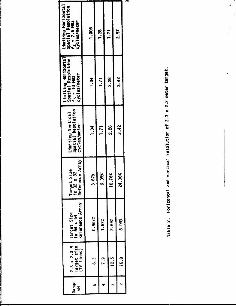
Consider a 525 line TV system with approximately 480 active lines

and a 2° vertical FOV. A standard 2.3 x 2.3 meter target would subtend

6.3 lines in the TV FOV at 5 KM, 7.9 lines at 4 14, 10.5 lines at 3 KM,

and 15.8 lines at 2 KM. If the reference array is 64 x 64 (in a

full-frame correlator), then the target occupies 0.967% of the refer-

ence array area at 5 1K4, 1.52% at 4 1(M, 2.69% at 3KM, and 6.09%

at 2 KM. Therefore, it is evident that most of the correlation is being

performed on the target background and not on the target itself. If

the size of the reference array is 32 x 32, then the above target area

percentages would increase by a factor of four.

The results of the above paragraph can be stated in a slightly

diffarent way. If two TV lines are required to display a spatial cycle,

then the highest vertical spatial frequency detectable at 5 KM is 1.34

cycles/meter, at 4 KM is 1.71 cycles/meter, at 3 KM is 2.28 cycles/meter,

and at 2 KM is 3.42 cycles/meter. If the horizontal and vertical reso-

lutions are the same (i.e., sampling at 10 MHz) then the limiting horizontal

spatial fic ':ency resolution is the same as the vertical. If the sampling

rate is reduced to 7.5 MHz, then the limiting horizontal spatial

frequencies detectable are 1.005, 1.28, 1.71, and 2.57 cycles/meter

respectively at the above ranges. Stated another way, trees spaced

every 0.75, 0.58, 0.44, and 0.29 meters apart respectively at the 5, 4, 3, 2

KM ranges could be detected when sampling at 10 MHz while trees spaced

every 0.995, 0.78, 0.585, and 0.39 meters apart respectively could be

detected when sampling at 7.5 MHz. The above results are summarized in

Table 2.

C

4

V9- 4-P N

V) *.- U

C- -

-0

04'3

'C'0 5-

0

9- 4N.

50 0 -L- - (

E- 0

49-304'

.9 r- Ni--

N q. N r4.- kD W9

V)~ u 01

L..

a, . 4'5

4' M ') 0WNL C'(1O 0

c.9-

57

C. Preprocessing of Input Video

1. High Resolution Image Preprocessing

The purpose of preprocessing the HR video is to reduce the spatial

resolution of the HR video to that of the LR video, a condition necessary

for correlation purposes. This difference in resolution is caused by

the differing fields of view (FOV), number of TV lines per frame, frame

rate, aspect ratio, and sampling rate of the two TV systems. Due to

size, weight, and cost constraints the FOV of the missile seeker will

be W times (W>l) that of the FOV of the fine pointing and tracking

system. If W is an integer, then the preprocessor averages the first

W columns of the first W rows of the HR image to obtain the P(6,l)picture element (pixel) of the reference image. Then the next W columns

of the first W rows are averaged to obtain the P(l,2) pixcl of the

reference array as shown in Figure 16. If the sampled 1(R video forms

an A x B array, then the reference array is an (A/W) x (B/W) array. The

size of a possible target in the reference array is then identical to

the size of the target in the LR array. Equatior 63 is the preprocessing

algorithm where W is an integer.

W W 1 I A/wP(I,J) = HRN (63)W(-2 M=AIII 1HR[(WI-Wj

J B/W

The assumptions made in deriving Equation (63) are that both TV systems

have the same frame rate, same number of TV lines per frame, sae aspect

ratio, are sampled at the same rate, and have linear optics. Figure 17

illustrates in block diagram form the implementation of Equation 63.

The hardware implementation is presented and discussed in Chapter 4.

58

NI I

" -- P?2I----------

It I _ t-------------------

. - r L LII F, II 1

I Ia i I I I

I I I III I I

I I I Ii I I

I I o I I I I

Figure 16. Preprocessing of HR image where W = 3.

Sampled HR To comparitorVideo Scratch Pad Preprocessor

Control IHorizontal and vertical Sync

Figure 17. Block diagram of preprocessor.

59

If W is not an integer, the preprocessing algorithm is more complex.

Making the same assumptions about the two TV systems as made previously

and defining

U = smallest integer < (I - 1)W + 1

V = smallest integer - (J - 1)W + 1

X = smallest integer < IW

Y = smallest integer < JW

the preprocessing algorithm becomes:{x YP(I-j) I 2 HR(M,N)

w 2li=U+1 N=V+1

" (I-1)W HR(U,N) + Iw- X HR(X+1,NlN=V+1I'

+ I [ [ W] []N=Lt+l

[

+ [U- (I1)W] [ V - (J-1)W] HR(U,V) + [w - Y] HR(UY+1)]

+ [W-X] [V - (J-1)W] HR(X+1,V) + [W - Y] HR(X+1,Y+I)] (64)

Figure 18 illustrates rhe pixel averaging where W = 3.25. The algorithm in

Equation 64 can be check(ed by looking at the P(2,2) element in Figure 18.

60

SIj Z I I #

L -- -- -- -- -- - - --T -I r

L_.

Figure 18. Preprocessing where W 3.25.

The possibility that the last column and last row of P(I,1J) elements

turn out to have less than W x W elements of the HR array is of no concern

since only the 32 x 32 or 32 x 64 P(I,J) elements centered about the

desired target will be used in the correlation algorithm. The important

factor is to have the spatial resolution of the preprocessed HR array

identical to the spatial resolution of the LR array.

In Equation 64, W is the scale factor by which the resolution of the

fine pointing and tracking system TV image must be reduced. The scale

factor is due only to differing FOV and is the same in both the horizontal

and vertical directions because of the assum~ptions made about the two TV

systems. The effect on Equation 64 of removing thiese restrictions will now

be investigated.

a. Number of TV lines per frame.

If the number of TV lines in the HR image is twice the number of

lines in the LR image and all other factors are the same including the

FOV, then the vertical resolution of the HR image is twice the LR image

and the horizontal resolution is half. The reduction of horizonal

resolution is caused by the fact that the image beam is scanning twice

61

as fast in the HR image which causes each pixel width to be twice as

long when sampling at the same rate. This could be corrected by sampling

the HR image at twice the rate of the LR image.

Let WH refer to the horizontal scale factor and Wv refer to the

vertical scale factor between the HR and LR systems. Then if the ratio

of the number of TV lines in the LR to the HR images is WI and all other

parameters are identical, the contribution of the different number of

lines to WH is W1 and to WV is I/W1.

b. Aspect Ratio

If the LR infage has a 4:3 aspect ratio and the HR image has a 1:1

aspect ratio and all the other parameters are identical, then the vertical

spatial resolutions of the two sampled images are the same but the hori-

zontal spatial resolution of the HR image is 4/3 that of the LR ima.ge.

The reason for this is that with linear optics the LR horizontal line is

looking at a total scene which is 4/3 wider than the HR scene. However

since the scan rate and sampling rates are the same, then each pixel in

the LR image covers 4/3 as much horizontal target zea as the HR image.

Therefore the horizontal spatial resolution of the HR image is 4/3

greater than the LR image.

In general if the aspect ratios of the LR and HR images are P1 and

P2 respectively where PI/P2 = W2, then the contribution of the differing

aspect ratios to WH is W2 and to WV is 1.

c. Frame rate

If the frame rate of the LR image is 30 frames/sec and of the HR

image is 15 frames/sec and all other parameters are equal, then the

horizontal spatial resolution of the HR image is twice that of the LR

62

image and the vertical spatial resolutions are the same. This is caused

by the fact that the beam is scanning twice as fast in the LR system

thereby causing the spatial width of each pixel to be double that of

the HR image when the sampling rates are identical.

In general, if the ratio of the frame rates of the LR to HR system

is W3 and all other parameters are identical, then the contribution of

the differing frame rates to WH is W3 and to Wv is 1.

d. Sampling Rate

By an analysis similiar to that given in (a) - (c) above, if the

ratio of the sampling rates of the HR to LR TV images is W4 and all

other parameters are identical, then the contribution of the different

sampling rates to WH is W4 and to WV is 1.

e. Field of View

If the ratio of the LR to HR fields of view is V)5 and all other

parameters are identical, then the contribution of the different

FOV's to WH is W5 and to WV is W5.

f. General Spatial Resolution Matching Equation

If all of the parameters in (a) through (e) above are considered

at once, the total horizontal and vertical spatial resolution scale

factors are given by

WH = W1 W2 W3 W4 W5

(65)

W1I = W5/W1

63Defining

V a smallest integer < (I-1)WH + 1

V smallest integer<~ (J-1)WH + 1 )X - smllest integew < 1 I~

Y - smallest integer - JWH

the preprocessing algorithm given in Equation 64 can be placed in the

more general form given below.

I X YP(IJ) - M_ I NUI HR(M,N)

WHWV IMU1 NV+'

+ I [U - (I-1)W v] HR(U,N) + (IWv - X] HR(X+1,NN=V*I

Y r

+l ,o. [ I V - (J-1)WH] HR(MV) + [ JWH Y] HR(MY+I)J

+ [U - (I-l)wv] [ [V - (J-1)WHJ HR(U,V) + [JWH - Y] HR(U,YiI)I

+ [IWv - X] [IV - (J-1)WH] HR(X+1,V) + [JWH - Y] HR(X+1,Y+I)}

(67)

2. Low Resolution Image Preprocessing

Since the mean value used for quantizing each KxL sub-array in the

LR image is different, it is felt that all of the preprocessing can best

be handled digitally. This section presents the optimal and sub-optimal

techniques used to find the mean value and to quan1tize the pixels of each

KxL sub-array for the two level quantization case.

64

Optimlly for each value of p and q. in Equation 3 and figure 4 the

K x L pixels should be quantized about the mean video level of that sub-

array. This could be done by storing K lines of the low resolution video

in say 4 or 5 bit memry, computing the average value of each K x L

sub-array as each new pixel is added, then quantizing all K x L pixels

about the mean for each value of p and q. It is felt that this method

is far too time and power consuming for the amount of accuracy gained.

Several sub-optimal trade-offs will now be presented.

Since the mean video level is not expected to change appreciably

from frame to frame, one method of reducing the real-te computational

burden is to use the mean video level of each sub-array computed from

the previous frame. This ethod, however, requires additional memory

and additional host computer load.

A second possibility would be to quantize about the same mean for each

sub-array until the mean changes by more than some precomputed amount at

which time that entire K x L sub-array would be requantized about the new

mean. This method, however, still requires the hardware to requantize an

entire K x L sub-array.

A third possiblity is to store the previous K lines of digitized

video in 4 or 5 bit memory, compute the average value of each K x L

sub-array as a new pixol is digitized, and requantized only the last column

of the array about the new mean. This would require only K comparators

rather than KL comparators. The average can be computed ty storing the

sum of each column in shift registers. When a new pixel is added, the

first column sum is subtracted from the total and the column containing

the new pixel is added to the total.

65

A fourth possibility is to use the method of the previous paragraph

but quantize only the added pixel about the new mean leaving all other

quantized values the same. This would requiri only one comparator. Using

this method only the lower right pixel in the K x L array would be quantized

exactly as shown in the solid area of Figure 19. If the mean video is

assumed to vary linearly with distance from this pixel, then the upoer

left pixel has the largest error for this value of p and q. The fifth and more

accurate method on the average would be to compute the quantization level

of the marked pixel by computing the mean level of the dashed K x L array

as shown in Figure 19. This would mean a delay in each correlation

computation of approximately K/2 lines plus L/2 sample intervals.

-L-

k 'K

L' J

Figure 19. Method for pixel quantization.

The 'ixth possibility is to quaritize about the average of the HR

reference. It is felt that this method, while being by far the easiest

to implement, .ould lead to too many false registration points and would

be unacceptable.

A further study involving typical military scenes is needed to

determine which of the above trade-offs is the best to implement. Without

the benefit of this study, method five is recommended and an implementation

is suggested in Chapter 4 of this report.

66

3. Effect of Quantizatlon about Incorrect Mean

As pointed out in the previous section, one of the sources oi error

in the two level by two level (one-bit by one-bit) correlator is quanti-

zation about an incorrect r.an. The effect on the mean square signal/

noise ratio of quantizing an entire array about the same incorrect mean

is presented in this section. The effect on the ms S/N ratio of

quantizing each pixel about differing incorrect means is not presented.

However, the results can be used as an upper bound if one uses the

maximum expected mean error in the resulting curves.

Consider the HR and LR images quantized respectively with the

quantizers shown in Figure 20. These quantizers represent an error in

quantizing around the wrong dc level of the HR and LR images. Although

the above quantizers assume that the HR and LR signals are zero mean,

this does not necessarily have to be true. For HR and LR signals that

are not zero mean the dc error due to quantization wojuld be given by

AX1 X1-HR and AX2 = X2-L.

gl~x) g 2 (x)

1 12

X AXXX1 x X2 x

-i -i

Figure 20. Quantizers for the HR and LR images.

I m .

67

a. Direct Method

Conqider the ffrst line of video

L

R(1,q) I HR(l,m) LR(l,m+q) (68)M =l

Dropping the row 1 notation and quantizing the HR and LR signals as shown

in Figure 20 yields

AL

R(q) L m=1 g1 [HR(m)] g2 [LR(m+q)] (69)m=l

The variance in the estimate of R is

^2 A2

a^ = <R > <R> (70)R

where

A ( L<R>= E g [HR(m)] g2 [LR(m+q)] (71)

and 12<R > = m gl[HR(m)] g2[LR(m+q)]2)

Assuming sample pair independence, a gausian distribution of the

HR and LR signals, and evaluating the resulting expectation integrals

yields

2 1 - 16 erf 2 (J) erf 2 (i)} (73)R = 1

68

Using Price's Theorem to evaluate r(t) where p is the correlation

coefficient between HR and LR yields

dr C 2< agl H g 2 . (74)

Evaluating the partials in Equation 74 by inspection of Figure 20,

assuming a jointly gaussian distribution for the HR and LR signals and

2 2evaluating yields the following relationship between a and a.2P R

x 12 x22 7T- a 2

p = () e e 0^ (75)R

Substitution of Equation 73 into 75 yields the desired effect of the

incorrect mean on the ms S/N ratio.

x 2 22 1 I2 () (L--)2 xl 22)}p L -e e1 16erf (--)erf

(76)

b. SSDA Method

The registration function for the SSDA method is given by

1 L

R(q) = L Y IHR(m) - LR(m+q) I (77)m=l

Going thru an analysis similiar to that used for the Direct Method2

yields the identical result for a given in Equation 76. This was

expected, however, since the two methods have been shown to be equiva-

lent in the one-bit by one-bit case.

69

Figure 21 shows a parametric set of curves depicting the change in

2a for various values of (-..) and (x2). The dotted curve in Figure 21P

p2shows the effect on a, P if the dc errors in the quantizers are equal.

If both x and x are zero (i.e., no error in the mean), then12

Op2 x L = 2.467 which is the result obtained in Table 1. As can be seen

from Figure 21 the variance is essentially insensitive to small dc

errors but grows very rapidly for errors in the mean above 0.4a.

2a xL

p14 x /o=1.0

12- /XllCf=. 8

1 /c=. 6

x 1/cr=O

4- - -----

2-

.2 .4 .6 .8 1.0

x2 /r

Figure 21. Effect of do quantization level on the variance in theestimate of p

70

4. Preprocessing for Differing Sensor Characteristics

When trying to accomplish target hand-off between two systems. it

is very important for the two sensors to have similiar characteristics.

This of course is the reason for the necessity for the algorithm which

equalizes the spatial resolution of the two images as given in Section

C-1 of this chapter. It is also very important for the spectral charac-

teristics of the two sensors to be the same since correlation can be

accomplished only if the two video signals are almost the same. If one

sensor covers a wider frequency spectrum than the other, an optical

filter might possibly be used during correlation to cause the two

spectral responses to be the same. If the two sensors have completely

different spectral responses, such as one sensitive in the visible

spectrum and one in the infrared spectrum, then correlation would be

difficult to accomplish due to the difference in signal characteristics.

However one possibility in this case would be to preprocess the video

such that only the edges are used for correlation. This is a possibility

since even if there is a cont-ast reversal between the two signals, the

edges in the FOV should be approximately the same.

Preprocessing of the HR and LR arrays concerns changing the form

of the data so that a better registration between the two can be

obtained. In most of the literature that has been surveyed this task

is referred to as outlining, edge detection, or boundary mapping. These

methods are used mainly for cases in which the two images are acquired

at different times jr the images come from different types of sensors.

The first of these reasons is not applicable to the present system under

71

study. It is quite possible that for the system under study the timges

could be produced from different types of sensors. In this situation

the data representation of the ground scene from the two sensors might

be different. Then some type of preprocessing of the data, such as

boundary mapping could be employed.

Reference [5] describes a method by which boundary maps are pro-

duced from the raw data. Essentially this method calculates thedifferential change in magnitude from one data point to the next. It

does this for both X and Y directions away from the point being examined.

The algorithm then decides if the point being examined represents the

boundary of a region or not. If it is a boundary, then that location is

assigned a value of 1. If it is not a boundary point, a 0 is assigned

to the location. Once a boundary map is produced for the entire image,

a correlation can be performed using boundaries of objects in the image

instead of all the raw data from the image.

If the data received from the HR and LR imaging systems are of

different forms (such as would occur with different sensor characteris-

tics) then the method of boundary maps or edge detection would warrant

further investigation. Implementation of any of these methods, however,

requires additional hardware and computation time.

D. Vibration Analysis

The effect of LOS jitter of the PTS and missile seeker systems on

the correlation algorithm accuracy is investigated in this section. From

talks with MICOM engineers the jitter of the seeker LOS should be less

72

than 100 urad rms and is the value used in this section. The LOS jitter

of the PTS system has been demonstrated to be less than 30 prad for 3t

least one system. These values are the total rms jitter due primarily

to disturbances from the helicopter at 11, 22, 33, and 44 Hz.

The primary effect of LOS Jitter on the correlation algorithm is

to cause a distortion in the stoied video scene. For example, if the

jitter is causing the LOS to move downward during the sampling and

storage of a 32 x 64 element video array, then the 32nd line may actually

be looking at the scene the equivalent of several TV lines below where

it should be thus causing a stretching distortion. If the LOS is moving

up due to jitter, then the 32nd line may actually be looking at the

scene the equivalent of several TV lines above where it should be thus

causing a compressing distortion. The problem is further complicated

by the fact that one video image may be compressed and the other stretched

by the jitter. The net effect on the correlation algorithm is to cause

a smaller correlation peak which can be modeled by a reduction in the

sicnal-to-noise ratio

In the calculations which follow both TV systems are considered to

be 525 line systems with 480 active TV lines (the remaining 45 lines are

used in the vertical retrace), and to have 60 half-frames per second or

30 full frames per second (2:1 interlace) with a 4/3 aspect ratio. For

a sampling rate of 7.5 MHz the low resolution image will be digitized

into a 240 x 480 element array during the first half-frame and 240 x 480

element array during the second half-frame. If the correlator is designed

such that correlation values are calculated as data comes in, then correla-

tion is being performed during each half-frame (i.e., the 32 rows used in the

73

correlator all come from the same lf-frame). Therefore, the total

time elapsed from the first sample in each 32 x 64 array used in the

correlation algoritth to the last will be the time required to sample

31 complete lines plus 64 samples of the following line.

TR . 31 + (64/480) - 0.00197 seconds (78)

TR' 525 x 30

As stated previously the LOS jitter is predominately at 11, 22,

33, and 44 Hz. If one assumes that the 100 prad rms jitter is all at

44 Hz, the worst possible condition for correlation, then the greatest

angular disturbance which the LOS would have in 0.00197 seconds would

be twice the value of the 44 Hz sinewave evaluated at t = .00197/2

seconds.

A~max = 2(141.4) sin[2r44(0.000986)]

or

~max = 76.16 prad (79)

If the seeker vertical FOV is 20, then each TV line is scanning 72.7

prad if one assumes 480 active TV lines. Therefore the riaximum movement

of the LOS from the first to the last sample taken for each computation

of R would be slightly over one line. Since correlation in the half-

frame correlator is being performed by using alternate lines of the

full frame, it is felt that this amount of movement will not cause a

significant problem. A more detailed analysis could be obtained by

modeling this LOS movement with an additive noise source which would

degrade the S/N ratio.

74

Next consider the case where correlation is performed using 16 lines

from ore half-frame and 16 lines from the succeeding half-frame. The

32 x (A correlator then operates on 64 samples from each of these lines.

The total time required to samle the data used for each coqutation of

R is

TR 1 5 + 64 / 48 0 + 1 0.0176 seconds (80)

525 -30 60

which is more than half a cycle of a 44 Hz waveform. Therefore, the

total movement could be as much as the peak-to-peak LOS jitter or 282

prad. This represents approximately 3.89 TV lines. Even if all of the

jitter is at 11 Hz, the maximum angular movement would be 162 Prad which

is over 2 TV lines. Using the full-frame correlator the correlation

peak would be reduced more than for the half-frame correlator. The

net effect of the LOS jitter is a larg-r reduction in the S/N ratio for

a full-frame correlator than for a half-frame correlator.

Table 3 shows the maximum possible angular vibration in prad and

its equivalent in TV lines if a 100 prad rms jitter in the seeker LOS

is considered to be concentrated at i1, 22, 33, or 44 Hz. The data for

a 32 x 64 element correlator operating on each half-frame respectively

and for the same correlator operating on a full-frame are given. From

the data in Table 3 it is obvious that a 32 x 64 correlator operating

on successivie half-frames is much less sensitive to LOS jitter than a

full-frame correlator. The half-frame correlator is also simpler to

i mplent since data does not have to be stored from one half-frame to

the next.

1K= =

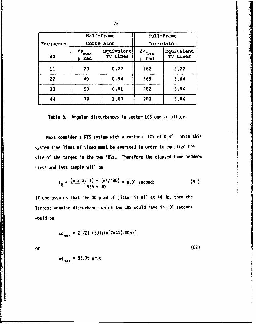
75

Half-Frame Full-Frame

Frequency Correlator Correlator

Afmax Equivalent A*max EquivalentHz j rad TV Lines p rad TV Lines

11 20 0.27 162 2.22

22 40 0.54 265 3.64

33 59 0.81 282 3.86

44 78 1.07 282 3.86

Table 3. Angular disturbances in seeker LOS due to jitter.

Next consider a PTS system with a vertical FOV of 0.40. With this

system five lines of video must be averaged in order to equalize the

size of the target in the two FOVs. Therefore the elapsed time between

first and last sample will be

TR = (5 x 32-1) + (64/480) = 0.01 seconds (81)

525 + 30

If one assumes that the 30 urad of jitter is all at 44 Hz, then the

largest angular disturbance which the LOS would have in .01 seconds

would be

Amax = 2(,f2) (30)sin[2w44(.0O5)3

or (82)

Amax = 83.35 Prad

76

For a vertical FOV of 0.40, each TV line, assuming 480 active lines,

scans 14.5 prad. Since each five successive lines of the PTS video are

averaged, the A~max is slightly more than one TV line when averaged.

The net effect of LOS jitter on the PTS is therefore seen to be

approximately the same as the effect on the seeker system.

E. Derivation of AX and AY Misalignment in LR Image

After the correlation array, R(p,q), has been calculated, it is

desired to move the missile seeker LOS such that the target is in the

center of the LR FOV. In order to do this the misalignment in both the

X and Y directions must be determined. The position of the target in

the LR image can be determined by performing a search of the R(p,q)

correlation array for a maximum in order to identify the registration

points p* and q*.

The geometrical layout of the HR and LR images is shown in Figure

22. The p and q counters start in the upper left corner of the LR

image. This designates the starting placement of the HR image in the

LR image for the calculation of the R(p,q) array.

Figure 22 also shows a possible location of the HR Image which

produced a maximum value of R(p,q) over all possible p and q. It is

desired that image registration take place in the center of the LR

image. The K x L array of LR image points around the center is shown

in Figure 23 along with the geometric definitions of AX and AY. The

displacements AX and AY represent values by which the LR camera must be

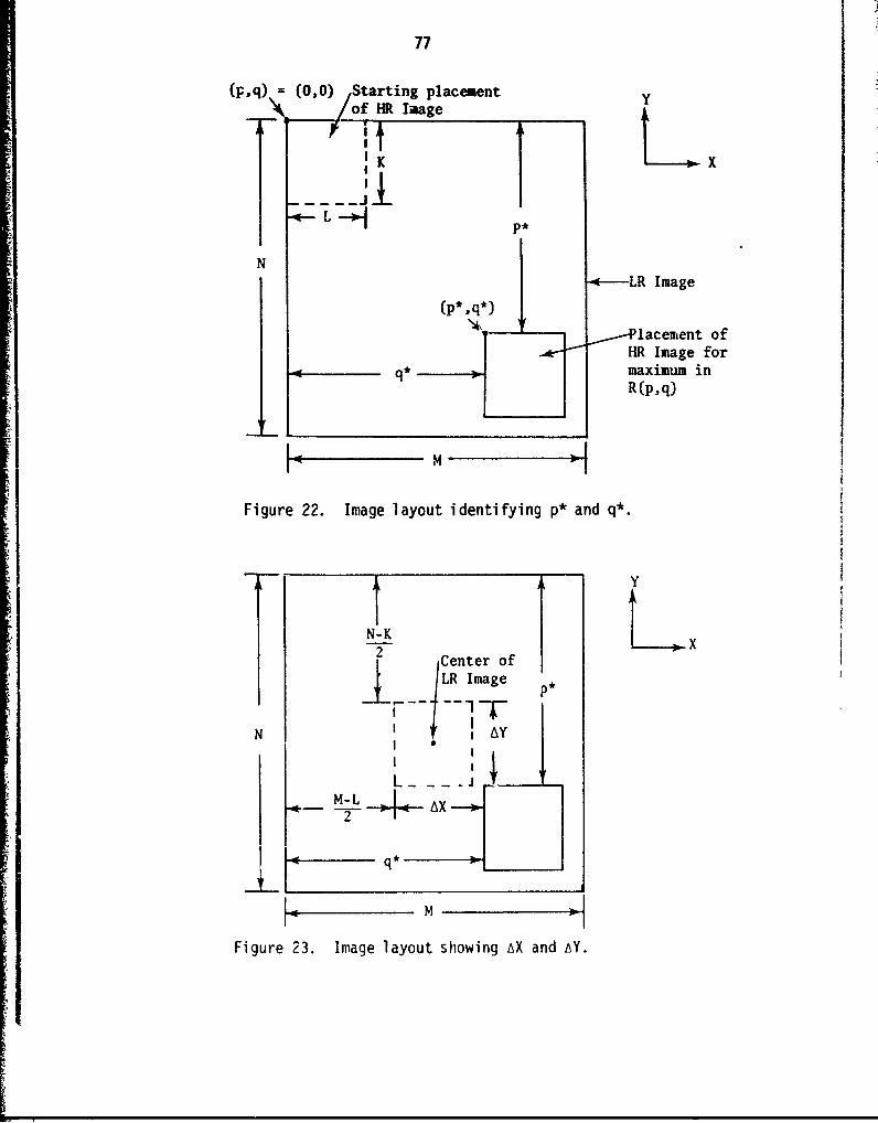
77

(p,q) (0,0) Starting placement/of HR Image f

K X

" "L -=*

N.0--LR Image

(p*,q*)

_--lacement ofHR Image for

q* maximum in

R(pq)

M

Figure 22. Image layout identifying p* and q*.

Y

N-K2 xN- /Center of

j 1 LR Image

N AN I * I £

L

M-L A2 A

q*

M

Figure 23. Image layout showing AX and AY.

78

shifted so that the maximum value of R(p,q) will occur at the center of

the LR image. It is desired that

p, = N - K (83)2

and

q, = M- L, (84)2

Using this reasoning AX and AY can be calculated using the following

equations:

AX= q* - (M-L) (85)2

and

AY =(-K) - p*. (86)2

The AY and AY in Equations 85 and 86 are expressed in terms of pixelelements. The angular errors A X and A¢y in a seeker with a FOV of 2',

480 active TV lines in this FOV and 480 samples per line are

AOX=480 x 20, in degrees (87)

= = "Y x 2°, in degrees (88)Ay 480

These angular errors can be used to torque the seeker gimbals such

that the target is in the center of the FOV.

79

F. Threshold Effects on Probability of FalseRegistration and Detection Probability

The following analysis develops the concepts of the probability of

false registration (i.e., the probability that two images are chosen as

registered when they in fact are not) and the probability of detection

(i.e., the probability that two images are chosen to be registered

given that they are in fact registered). Each of these probabilities

is given in terms of the tireshold for deciding if registration is

achieved and the input SNR for both images.

For simplicity and because other considerations 'ndicate its

desirability, the following is developed fcr a 1-bit by 1-bit (2-level

by ?-level) ,correlator using either the Direct Double Summation Methud

or the Sequential Similarity Detection Algorithm. Previous comparisons

have shown these two methods to be identical statistically for the 1-bit

quantization case.

The ollowing assumptions are inherent in the devopment.

1. Signal and noise levels at each pixel are independent oF each

other and of signal and noise levels from any other pixel.

2. The noise at any pixel is zero mean Gaussian for both the HR

and LR images.

3. The rms noise level is constant (a nHR) for each pixel of the

HR image and a different constant (a nLR) for each pixel of the LR imag?.

4. The signal levels for the HR dnd LR images have mean values

HR and [R respectively for thp pixels within each image. It is of course

realized that ER may change as p aid q (the shift values) change; however

for a gien correlation comnpt&tion LR is a cot:tant.

80

5. The signal plus aaditive noise from HR and LR images are

subjected to 1-bit quantization as represented by g, and 92 in Figures

24 and 25.

The only possible outputs for a one-bit implementation are zero or

one for comparison of a LR pixel with a HR pixel. Therefore, for

implementation of a K by L. array correlation, the correlation magnitude

takes on values ranging from 0 to KL in integer steps. The ovvious

questions which arise and the answer of which is the purpose of this

section is: "How close to the maximum value of KL must a given corre-

lation be to indicate registration? What are the consequences of

chosing a particular threshold for a decision on registration of the

HR and LR images?"

Under the assumptions outlined above we can write the probability

density functions for the noise in any pixel of the HR and LR images

for a given shift value (p,q).~2

-nHR

f 2anHR (89)nHR R a

2

22 nLR

f kn -e (90)n LR) LR

At pixel (n,m) in the HR image and pixel (n+p, m+q) in the LR image we

have signal plus noise as follows:

rHR = rHR (n,m) = HR(n,m) + nHR(n,m) (91)

81

r HR(n,m) + n (nm)rHR HR'

rL= LR(n+p~m+q)+n (n+p,m+q)

92 0. 92(r LR)

input =signal + noise quantized output

Figure 24. Quantized signal plus noise.

M1(rR)

rHR

g 2(r LR

- rL

Figure 25. Quantizer characteristics.

82j

r LR r LR (n+p. m+q) =LR(n+p,ni+q) + nL np m+q) (92)

where rHR and r LR are to be quantized and compared logically and the

output summned for KL pixels as shown in Figure 26.

rHR grHR)I LOGICCOMPARISON (1 if match)

r g(r~)(01 PIXEL) 0match) CORRELATIONLR 92L) (0 to KL)

Figure 26. Correlation technique.

From the quantizers g, and 92we have the rules for no noise

g I i f HR > HR

0 Oif HR <HR-

92 1 i f L R > I R

0if LR < LR

If noise is included, the rules become with noise

g : 1 i f HR+nHRHR (95)0if HR+n HR < R

92 1 if LR+n LR > LR

0 -J LR+n LR <Of(96)

83

Clearly there are four hypotheses that can be postulated for the

outputs of the two quantizers in terms of the inputs. The

hypotheses are:

HHRO - the input HR < -R (choose gl=O)

HHRl - the input HR > HR (choose gl=l)

HLR0 - the input LR < LR (choose 92=O) (97)

HLRl the input LR > LR (choose 92=l)

These hypotheses can be chosen with no error by a simple threshold

circuit if no noise is present. If noise is present, there are possi-

bilities for error in the choices. This error is dependent on the signal

levels, the noise statistics and the number of pixels used in a given

correlation computation.

The correlation output is then compared with a threshold value, NO,

to determine if the images are registered. If the correlation output

is greater than NO, the images are chosen to be registered. Since No

is a para.ieter which must be chosen, its effect on expected errors must

be known. Specifically its effect on false alarm and detection proba-

bilities must be Vnown.

1. False Alarm

False alarm occurs when the logic comparison indicates registration

of the image with a particular LR image when in fact the two are different.

The probability of false alarm is best examined by considering the

probability of false alarm for each comparison of an HR and an LR pixel

84

pair. Defined for each pixel pair, the false alarm probability is

simply the probability that the HR and LR pixels are chosen matched

given that they are different. However, since the WR and LR images

can be different (not registered) without requiring that all KL pixels

be different between the two images, consideration must be given for

the probability of matched pixel pairs within non-reqistered images.

This consideration requires an additional assumption about the proba-

bilities of pixel pairs being matched or mis-matched given that the

images are different. Fortunately, based on fundamental arguments

supported by the method of quantizing about the mean value for each

image, these assumed probabilities are easily obtained.

Since the relation of total number of chosen pixel matches to the

threshold No is really what determines false registration probability,

it is necessary to examine the probability of coosing pixels as

matched given that the images are different. Clearly this has two

parts: 1. probability of [choosing pixels matchedlpixels matchedi

images different], and 2. probability of [choosing pixels matchedi

pixels different limages different].

If the individual pixels for different images are assumed to be

independent of each other, then a "0" or "1" is equally likely at any

given quantization step. This should be true for any symmetric proba-

bility density functions of the HR and LR intensities since quantization

is about the mean value in each image. With this assumption, it can be

shown that for each pixel pair comparison, the probability of false

alarm is independent of the image signal-to.-Aoise ratios.

85

The probability of false alarm for the ith pixel pair comparison

is

P i[E] = [MHRMLR + (l-MHR)(1-MLR)] (98)

•P[pixels matchidifferent images]

+[(l-MHR)MLR + MHR(1-MLR)]'P[pixels differentlimages different]

where: SNRHR 2J -MHR f-7

2NRLR

MLR e T do

SNRHR = HR image signal-to-noise ratioSNRLR LR image signal-to-noise ratio.

Under the assumption stated above P[pixels matchlimages different]

: P[pixels differentlimages different] and Pi[E] = ; for all SNRHR

and SNRLR.

If all KL pixels are considered, we find that if N is the number

of false alarms in KL pixels then the probability density function for

N is given by

( E] KL\ N b(KL-N) (99)PNE] N a

where PN[E] is the probability of exactly N false alarms and obeys the

familiar binomial probability law j

86

where = (KL)! (100)N! (KL-N)!

is the binomial coefficient and gives the number of possible combinations

of KL pixels with N false alarms, and

a = Pi[E] = probability of false alarm, on each pixel pair

b = I - Pi[E].

If a threshold value of N is chosen, i.e. N = No, such that if

N < N0 for any given correlation computation the decision is to reject

the hypothesis that the images are alike, then a probability of false

registration can be found as a function of N0 from

PFA[NO] = Probability [N > Nolimages different]

orN

PFA[No] = 1 _L()K/ aN,(KL-N) (101,N= 0 N

For KL large, the binomial probability law is approximately gaussian

which givesN - (KL)a +

-(KL)ab

where

e 2

M(x) L e 2 d .

87

Probability of false alarm is plotted versus threshold, N0, for

KL = 2048 in Figure 27 and for KL = 1024 in Figure 28.

2. Detection

Detection or correct registration occurs when the HR and LR images

are correctly chosen to be identical; that is, they are chosen matched

given that they are matched. Similar to the development for false

alarm, it is convenient to start with a single pixel pair comparison to

derive the statistical behavior of correct registration.

The major difference between the probabilities for false alarm and

detection lies in the fact that when the HR and LR images are registered,

the probability that pixel pairs match should be higher than it was for

the unlike images examined in the false alarm treatment. Furthermore,

this difference in probability of match and mismatch for each pixel

pair results in the probability being dependent on signal-to-noise

ratio's of the two image signals.

The probability of choosing a pixel pair matched given that the

HR and LR images are registered is

P.[C] = [MHRMLR + (1 - MHR)(l - MLR)]

•P[pixels matchlimages same]

+[0l - MHR)MLR + MHR(l - MLR)]

*P[pixels mismatchlimages same] (103)

4

0C ~88CC)

0~0

C))

-)

o C)

C) 0)

C Cs

LL--

C) V)

00

- ~ ~4-)

.0

C7% 1 - 4 - -4 -0N C)

N I333 JOA-IV0d dv

WdVIV3SIV JO IIII~ dd0

89

00

-- 0 0v

le 0

CD 4

0

C))

0

u; .1

CL cu

4.)

In

0 0 L

0 CD

L.f

0) C)

CT) 0) C

C) LA 0 ) 0 C

CD aNOII3i~ 30 A AO~dd d 0

WdVIV3SIVJJO Alllg~.dd-

90

or if we define the error probability

SA P[pixels mismatchlimages same)

then

Pi[C] = [MHRMLR + (1 -MHR)(l -MIR)] (1-)

+(0 - MHR)MLR + MHR(l - MLR)] c (104)

For the ideal case, e = 0, each HR and LR pixel pair will match so

that additive noise is the only error source. However, for practical

sensors, there is a finite probability that pixel pairs will mismatch

due to different spectral responses, non-linearities and other error

sources. Thus it is important to examine the effects of non-zero

values for c. Since MHR ano MLR are dependent on signal-to-noise ratios

SNRHR and SNRLR of the respective video signals, then as indicated by

Equation 104 the probability of choosing a single pixel pair as being

matched, given that the two images are alike, is dependent on the three

parameters SNRHR, SNRLR and c.

Once the value for Pi[C] is established then the total detection

probability as a function of the threshold, No, can be determined. If

all KL pixels are considered, we find as with the false alarm problem

that if N is the number of pixels chosen as matched, then the probability

density function for N is again binomial.

PN[C] = (KL) N d(KL-N) (105)

..N

91

And the probability of detection is the probability that N will be

greater than No , or

PD[NO] = Probability [N > Nolimages alike]

N0

PD[No] = I - YO KcN d(KL ' N) (106)N=O

where

c = Pi[C]

d = 1 - Pi[C]

Clearly, PD is a function of KL, N0 and Pi[C] which in turn depends on

SNRHR, SNRLR and E. Figure 27 shows PD versus threshold, N0, for

KL = 2048 data points and for three worst case values of Pi[C]. (NOTE:

Pi[C] is listed as PIC on all figures).

A value of PIC = 0.5 gives exactly the same curve for PD as is

shown for PFA" This could occur only if we assume a value of c = 0.5.

This is highly unlikely since it says, that even thougn the images are

alike, there is at best a 50-50 random chance that individual pixel

pairs matci between the two images. If the sensor characteristics are

so different that E < 0.5 is possible, then there is no need to waste

effort trying to correlate the two indges. Figure 28 shows similar

curves for PD with KL = 1024.

As an example of what the curves in Figures 27 and 28 mean consider

that it is desired that a high PD be attained while keeping the number

of false detections to one rer second. The number of false detections

is given by

92

NFD =PFA * NpNq * F Tm

where:

N = number of shift values "p" for which correlationis computed

Nq number of shift values "q" in the other direction

F = frame rate (frames/sec)

Tm = total mission time (I sec)

NFP = PFA " [640-64][480-32] • 30

(107)

1 8(10 6 )PFA

which requires PFA < 1.2(10-7). Then from Figure 27 this PFA corresponds

to a threshold of N0 = 1140.

Projecting up to the PD curve for PIC = 3.55 indicates a detection

probability of less than 0.3 which is unacceptable. For PIC = 0.5 the

value of PD is greater thai, 0.9999. Evaluation of this result says

that if a false alarm rate of one per second is to be achieved then to

maintain high detection probability, SNRIR, SNRLR and s must be such

that PIC > 0.55 and preferably > 0.6.

The relationship between PD and PFA is shown more clearly in Figure

* 29 where NO is the common variable which has been removed. Improvement

in performance is represented by movement of the curves diagonally

upward from the coordinate center.

Incidentally, a false alarm rate of one per second is the case

where one false registration occurs out of -8(106) correlations.

This is the number of real time correlations computed per second for a

934

co

a- #

0 0 EU C11T 0C- tCD CA.

bza a. 4

4--E0 0 i

LO II

C.I.)

0 L

C)CCN-

0) C0

a). m I

cOL

N0110130 o AIIIGVs-d

94

32 x 64 reference array and a 480 x 640 low resolution image at standard

TV frame rates.

Since the above results are so strongly dependent on PIC a parametric

analysis of PIC is of value.

The effect of c on the value of PIC is shown in Figure 30 for four

discrete values of c as a function of signal-to-noise ratio. For

convenience in plotting, only values corresponding to equal SNR for the

video signals are shown. The figure shows that c has a profound effect

on the maximum attainable value of PIC which is reached asymptotically

as the signal-to-noise ratios increase. In each case, the maximum

achievable value of PIC is 1-c, and is achieved only as the two video

SNR's increase.

Since the HR image SNR and the LR image SNR will most likely vary

independently of each other, it is of interest to examine the effect of

different SNR's on PIC. Figure 31 illustrates this effect for a fixed

value of c = 0.1. As in Figure 30 the absolute maximum attainable PIC

is 1-c; however, it is not reached unless both video SNR's are greater

than 3. The point made by Figure 31 is that for optimum detection

probability, both images should have a SNR of at least three. Only

partial compensation is achieved by one video signal having very high

SNR if the other video signal has SNR significantly less than 3.

To summarize briefly, the above analysis indicates that for

signal-to-noise ratios which can reasonably be expected from electro-

optic sensors (-3), even for a worst case assumption about sensor

characteristic mismatch (c = 0.4), for the 32 x 64 reference array size

Il ii i iiillli i lm m nl i i.. . .. . ..... ..

0.9 9

0.8

0..7

0.6

0.5.0.0 1.0 2.0 3.0 4.0 5.0 6.0

SNRHR SINRLR

Fiqure 3o. Effect of SNR and pixel mismatch probability, ,on

probability of a correct decision Pinr each pixel.

0.9-SRR> 3.0

0.7 -- 0.

0.6-

SNRHR =0.0

0.5 I0.0 1.0 2.0 3.0 4.05. 6.0

SNRLR

Figure 31. Effect of different video SNR on probability of

making correct decision for each pixel.

97

a threshold can be set which will ensure low false alarm rate and high

detectio probability. It should be stated that the above analysis is

based on a one-look correlation for each shift value. Multiple-look

correlation, that is, computing the correlation function for a given

shift value several times and using a decision based on the multiple

correlations, will provide even better performance statistically. How-

ever, since multiple correlations in real time would require parallel

processors, increased processing sperd or reduced data array size, that

technique can be eliminated for practical reasons. More than adequate

statistical performance should be achievable with the one-look real-time

correlation technique.

G. Target Not in Seeker FOV

Due to inaccurate boresight alignment or to movement of the missile

within its stores rack, there exists the possibility that the target

will not be within the seeker FOV. If the correlation coefficient does

not exceed the threshold value during n consecutive TV fields, the

decision is made to slew the seeker TV LOS -in a search pattern to find

the target. The value of n is a design parameter which should be

studied in a technology program. A value of from one to four would be

an adequate range for such a study.

Figure 32 illustrates two possible search patterns. Figure 32(a)

shows a search pattern which searchs for the target over an area which

is nine times the area of the original search area in eight discrete

steps of the seeker LOS. Figure 32(b) shows a search pattern which

searchs for the target over an area which is four times that of the

98

r . . . . . .r - - -

I I1 Ii

4 3 2I III - - -. ..-

I 5

I I --

6 7 8! I

i I

(a)

2II 1I2 II

3L __ 4 i

i I i

S I I

I I II - - ' j II I IL3 -. -_L. _ 4j

(b)

Figure 32. Search patterns for missile seeker.

L__

99

original area in four discrete steps. Search pattern 32(b) would

require less than half the time as seerch pattern 32(a) if say the

target is in the last possible dotted square. Due to recent experiments

conducted at MICOM where the missile seeker was slaved to the PTS,

it is felt that the search attern of Figure 32(b) will be adequate

(i.e., the probability of finding the target in search pattern 32(b)

is quite high). However, in a technology program, tests should be

conducted to determine the optimal search pattern (that is one that

yields a high enough probability of finding the target in the least

possible time). Another reason for choosing search pattern 32(b) is

because of the iaccuracies of the correlation algorithm around the

edges of the FOV. Since the edges of the original FOV in Figure 32(b)

are well within the search pattern FOVs, the possibility of missing

the target due to edge effect is reduced. If one uses the search

pattern of Figure 32(a), there exists the possibility of not finding

the target at all even though it is within the original FOV but close

to an edge.

The correlation values are ignored during the slewing of the seeker

LOS. When the LOS stops, if after n TV fields the correlation does

not exceed the chosen threshold, the LOS is advanced to the next search

area. If after completely searching all areas the threshold is not

exceeded, the gunner would be flashed a sljnal to this effect whereupon

he can re-initiate the process if he desires.

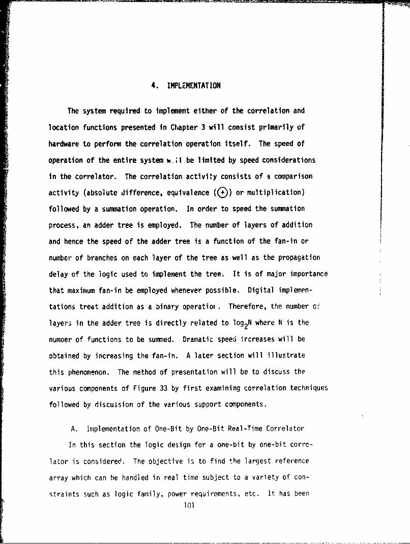
4. IMPLEMENTATION

The system required to implement either of the correlation and

location functions presented in Chapter 3 will consist primarily of

hardware to perform the correlation operation itself. The speed of

operation of the entire system wo;I be limited by speed considerations

in the correlator. The correlation activity consists of a comparison

activity (absolute difference, equivalence (cD) or multiplication)

followed by a summation operation. In order to speed the summation

process, an adder tree is employed. The number of layers of addition

and hence the speed of the adder tree is a function of the fan-in or

number of branches on each layer of the tree as well as the propagation

delay of the logic used to implement the tree. It is of major importance

that maximum fan-in be employed whenever possible. Digital implemen-

tations treat addition as a binary operatior. Therefore, the number c'

layers in the adder tree is directly related to log 2N where N is the

numoer of functions to be summed. Dramatic speei ircreases will be

obtained by increasing the fan-in. A later section will illustrate

this phenomenon. The method of presentation will be to discuss the

various components of Figure 33 by first examining correlation techniques

followed by discussion of the various support components.

A. Implementation of One-Bit by One-Bit Real-Time Correlator

In this section the logic design for a one-bit by one-bit corre-

lator is considered. The objective is to find the largest reference

array which can be handled in real time subject to a variety of con-

straints such as logic family, power requirements, etc. It has been

101

102

'Lou

0U

CL0

4J

E rE tOi

40~

00

Ir--- OOF-P0

to

I'-0d4

>W 4J

cc im 4)

m LL C> C

V9

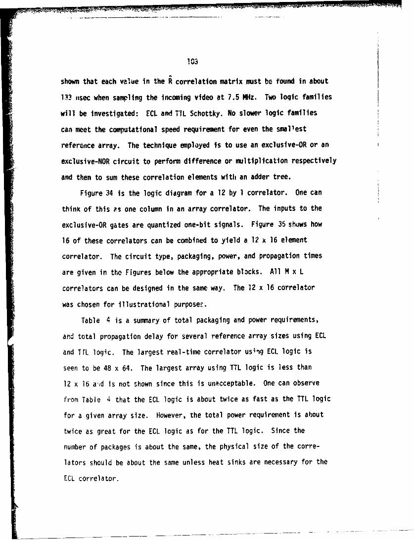
shown that each value in the R correlation matrix must be found in about133 nsec when sampling the incoming video at 7.5 MHz. Two loqic families

will be investigated: ECL and lL Schottky. No slower logic families

can meet the computational speed requirement for even the smallest

reference array. The technique employed is to use an exclusive-OR or an

exclusive-NOR circuit to perform difference or multiplication respectively

and then to sum these correlation elements with an adder tree.

Figure 34 is the logic diagram for a 12 by 1 correlator. One can

think of this is one column in an array correlator. The inputs to the

exclusive-OR gates are quantized one-bit signals. Figure 35 shows how

16 of these correlators can be combined to yield a 12 x 16 element

correlator. The circuit type, packaging, power, and propagation times

are given in the Figures below the appropriate blocks. All M x L

correlators can be designed in the same way. The 12 x 16 correlator

was chosen for illustrational purposes.

Table 4 is a summary of total packaging and power requirements,

and total propagation delay for several reference array sizes using ECL

and TrL logic. The largest real-time correlator us-ig ECL logic is

seen to be 48 x 64. The largest array using TTL logic is less than

12 x 16 a' d is not shown since this is unacceptable. One can observe

from Table 4 that the ECL logic is about twice as fast as the TTL logic

for a given array size. However, the total power requirement is about

twice as great for the ECL logic as for the TTL logic. Since the

number of packages is about the same, the physical size of the corre-

lators should be about the same unless heat sinks are necessary for the

ECL correlator.

104

MC101 7 MC 0180MC10 82 M 10484pkg2pkg2pkgI pk

480 W 72 MW1150 MW 6 0 M2.5 S 4. NS7*5 S 6. 4J

Figure ~ ~ ~ ~ ~ C V~*Lgcfr12x1creao

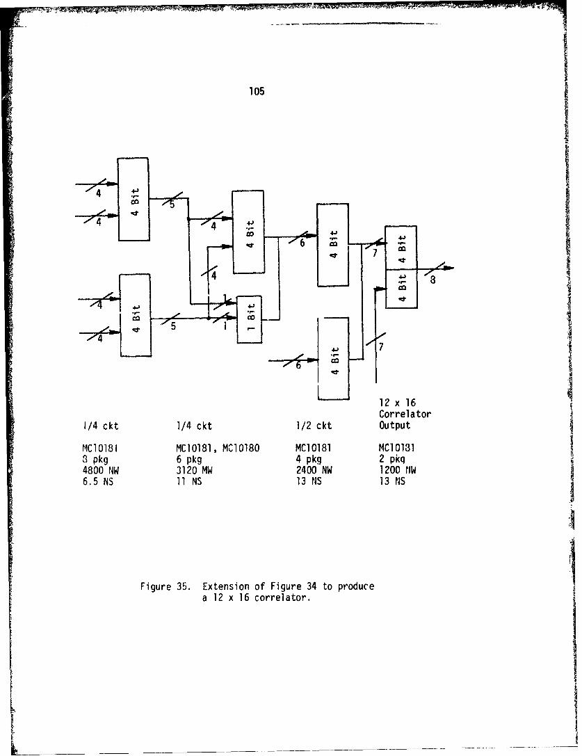
105

-fj

3pg 6pk 4p#- 2pk

a ~~12 x 16corlt.

106

ECL TTL

Array Size Pkg Power Delay Pkg Power Delay

8 x 12 82 29 W 51 ns 74 15,W 114 ns

12 x 16 166 59 W 64 ns 150 30 W 139 ns

16 x 24 366 120 W 77 ns 304 61W 164 ns

24 x 32 671 239 W 90.5 ns 611 123 W 189 ns

32 x 48 1345 480 W 108.5 ns

48 x 64 2696 964 W 126.5 ns

Table 4. Comparison of ECL vs. TTL logic correlators.

It is possible to extend the hardware in a simple way to encompass

larger arrays with little increase in hardware complexity. The basic

design of all the fast correlators is a multiply circuit and an adder

tree. In the one-bit case it is possible to "hang" additional multiply

circuits on the adder tree without effecting the propagation times

considerably. The full adder is in fact a ternary function. Figure 36

shows the logic diagrams for a 15 x 1 correlator. Figure 37 is the

exteihsion of Figure Jo that produces a 15 x 16 correlator. This basic

block is iterated in space to form the various array sizes listed in

Table 5.

107

4J I-

4- MCO3XO2Coilo BtAde2VC08 i de

21Mlll4 i de

prpaato deav1NV oe 25M

______2 -. i.. aeshngo te

Figur 36. ogic iagrm ford 15 1 on-bit CeAor

I<

410

7 re ato

1/4 c14/4ct 12 k Otu

15~~~1 x 116oteatr

109

ECL

Array Size Pkg. Power Delay

15 x 16 166 59w 64NS

16 x 30 366 120w 77NS

30 x 32 671 239w 90.5NS

32 x 60 1345 480w 108.5NS

60 x 64 2696 964w 126.5NS

Table 5. One-bit by one-bit correlator usingECL logic.

It appears unlikely that a complete ECL Implementation would be

practical due to the large power requirement. In this section we will

first describe an implementation based on low power Schottky TTL-logc.

Since this logic family is not fast enough to do an addition of 2048

(32 x 64) one-bit numbers in anything apnpraching 133 ns, it is

necessary to perform the computation in pieces. This technique is called

pipelining. During a giver time interval the 'pipe' may be computing

Part 1 of Item 3, Part 2 of Item 2 and Part 3 of Item 1; at the next

time step computation is performed on Part I of Item 4, Part 2 of Item

3, Part 3 of Item 2. A ned result is generated at eachtime interval but

for any specific data item the time required is the product of the basic

time interval and the number of sections of pipe (see Figure 38). The

Schottky pipe version illustrated on the accompanyin5 pages (Figure 39)

requires approximately 1600 packages and 300 Watts for a 32 x 64 array.

110

p 1 p2 p 3jtime

1 1

1 3 12 I

I 12 I1 done

15 14 13 12 done

Figure 38. Items in pipe.

The pipe delay in each of the three sections of pipe is 132 ns.

Memory required in addition to that contained in the correlator itself

is assumed to be a charged coupled device since this will provide the

necessary speed with very low power consumption. Bubble memories may

become practical in this application as well. Assuming a picture image

P x Q with R points devoted to horizontal retrace and sync, and a corre-

lation array K x L, from Figure 40 we observe that the delay required is

(Q + R - L) for each row. Using CCD (charge coupled array) power dissipa-

tion at 10 MHz is about 20 PW/BIT. Therefore total power dissipation is

20 x 10 3K(Q + R - L) mllliwatts.

.0 OOP 4. c

~ 0 8

4) 4

I.- a 4t-

ino viv

r* InL

4)I.-

fil viva

Ino viva

112

044..1

4.)1

00

I.- iCC

q. 00

O.

0c

a.N

F. C~ noE.

113P,

10 4004-

C

InI

LLL

C-l

L 4

A mcin.

114

1 9

c

10

4.4.

m C

53 0p

Ioo

115

Q R

L

|L A(Q + R - L) Bits each row

K(Q + R - L) Bits total

Figure 40. Memory requirement for correlation computation.

Another problem involving the one-bit by one-bit correlator concerns

the removal of the DC component of the LR image. This forms a support

component in the system block design. The following is a discussion of

a sub-optimal technique that accomplishes the removal of the DC digitally.

Referring to Figure 41, in approximating the level about which to quantize

pixel A the value of pixel B must be known. Pixel B lags A by (K/2)(Q+R) +

112 sample intervals. The column containing pixel B is used to determine

TKLK2

Figure 41. Method of computing mean video level.

116

L man values and then is not used until Q + R - L events later. Data

Item C must be removed from the column sum after K(Q + R) events. The

resulting algorithm is presented as Figure 42. If we assume a 3 bit

quantization of the picture, then 3 x [K x (Q + R) + L/2] + 14 x (Q + R + L)

bits of emory are required As before, using Q + R -476, K = 32, L-64,

53,352 bits are required. Power dissipation is approximately 1.5 watts

for the memory array using CCD. Clocking and interface logic could increase

this number significantly.

Mean Value(Shift to divide

Data.- G1 Bi (3 Bit)

Comparator

3x (K(Q + R) + L/2)

+ 14x (Q + R + L) Bits of memory

Figure 42. Mean video computation and quantizer.

117

The use of half-frame correlation (i.e., non-interlaced images)

serves to reduce the hardware memory -equirements. In order to achieve

reasonable computational speeds through the adder tree, the circuit is

divided into sections (i.e., pipelined). With Interlacing, one of the

final stages of the pipe sums results delayed from the previous half-

frame. Because this delay requires considerable memory and because

of the effects of vibration discussed earlier, it is recommended that

a hb2f-fra;ie correlator be implemented, thus, effecting a cost, space

and power saving,

The maximizing circuit is quite simpie and is shown in Figure 43

The position counter is also used in the edge correction problem. The

picture is dimensioned as in Figure 44 . )lotice that both the hori-

zontal and vertical blanking intervals are indicated by a one in the

most significant bit of each counter. The retrace intervals have been

adjusted to ensure this simple hardware implementation. The final

construction may require that sample rates be adjusted to achieve this

effect.

The mean value of the image needed for quantization near the edges

is difficult to calculate because part of the K X L subarray extends

into the horizontal retrace region or vertical retrace region as shown

in Figure 45. The dc component of these areas that depend on values

outside the field of view can be calculated by substitutinq a binary

noise source for the retrace voltage. One possible implementation is

shown in Figure 46. This will preclude the possibility of false con-

trast changes near the edge by smearing the edge so that it always

appears gray.

118

IV 004J L.

00 4) .'04 1, 4

c 411S..Z1 Ll 410 0 1-4

0) 441

1. Im-L.40 C) 4.3

00

ro Ln%

cm 04) 0)

x cmc~

04~~ (Mto4

cc c

119

RA

P

S

P x Q is single scan picture area

For example 256 x 512

R and S are horizontal and verticalblanking intervals

For example (P + S) x (Q + R) couldbe 320 x 576

Figure 44. Picture size (P x Q) with horizontal andvertical retrace R and S.

*1

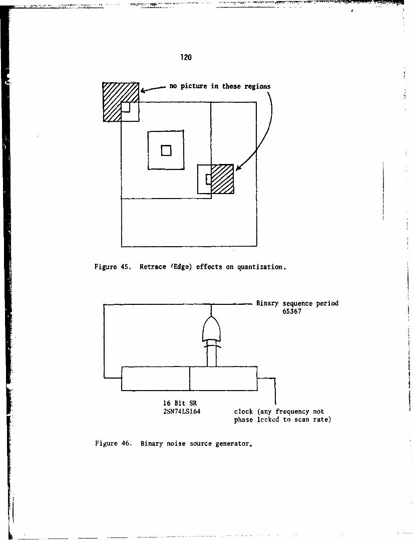
120

no picture in these regions

Figure 45. Retrace (Edge) effects on quantization.

-Binary sequence period65367

' Z iI

16 Bit SR2SN74LS164 clock (any frequency not

phase lccked to scan rate)

Figure 46. Binary noise source generator.

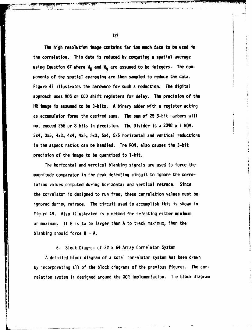
121

The high resolution image contains far too much data to be used in

the correlation. This data is reduced by copputlng a spatial average

using Equation 67 where WH and W are assumed to be integers. The com-

ponents of the spatial averaging are then sampled to reduce the data.

Figure 47 Illustrates the hardware for such a reduction. The digital

approach uses NOS or CCD shift registers for delay. The precision of the

HR image is assumed to be 3-bits. A binary adder with a register acting

as accumulator forms tke desired sums. The sum of 25 3-bit ,tumbers will

not exceed 256 or 8 bits in precision. The Divider is a 2048 x 1 ROM.

3x4, 3x5, 4x3, 4x4, 4x5, 5x3, 5x4, 5x5 horizontal and vertical reductions

in the aspect ratios can be handled. The ROM, also causes the 3-bit

precision of the image to be quantized to 1-bit.

The horizontal and vertical blanking signals are used to force the

magnitude comparator in the peak detecting circuit to ignore the corre-

lation values computed during horizontal and vertical retrace. Since

the correlator is designed to run free, these correlation values must be

ignored durin retrace. The circuit used to accomplish this is shown in

Figure 48. Also illustrated is a method for selecting either minimum

or maximum. If B is to be larger than A to track maximum, then the

blanking should force B > A.

B. Block Diagram of 32 x 64 Array Correlator System

A detailed block diagram of a total correlator system has been drawn

by incorporating all of the block diagrams of the previous figures. The cor-

relation system is designed around the XOR implementation. The block diagram

122

CM

0 cm

CM

*q In -

I. VC1 of

+

<00

4.- 1

I-IA

44

Li C)

= V;Ln 0

41 #aCLL

c 4.)

cyI-

123

Next Next4 NSB 4NSB 4 Bits 4 Bits 4 LSB 4 LSBof B ofA of8 ofA of B of

, a

s min axab B<A 8,BA B<A

BlnHrz -- V :,;B>A +AT: a AB BA

- Sc e B-A_ B-A

Vert

Blank

Figure 48. Blanking circuits for correlator duringhorizontal and vertical retrace.

also shows the pre-processing that is done on botit the HR and LR video

signals assuming an adjustable FOV ratio between the two and also shows

how the processed signals are clocked into the correlator.

The completed implementation is shown in Figure 33. A more detailed

representation is shown in fold out Figure 49. It is important to remember

that the diagrams represent potential ways of implementing the desired

design and are presented as a feasibility demonstration. A practical

implementation might not employ identical techniques. The following

discussion treats the blocks in Figure 33 as a system. The component

functions were treated separately earlier in this chapter. The high

r- HinPasF ter1

ITI

Hig Reouto I

Video Inhiit

compos i tie ResetVideo 'a 7w193

High Resolution Clamper anld PelOd6 Reference ArrayCamera Sync Stripper every 16th frame

Narrow HR SyncFOV

Sync Gens, y- I.andI

DeflectionAmipl ifiers2

Cockpit 20 CeConMoni tor Ire

Sync Gens.and

DeflectionAmplifiers !is,,p*I (,c k(

125

- 114R Data In

~1IF1

I HR Clock

sIti_Resolution Peducer

See Figure 47

Inhibitltest

TR N

d Reference Arrayy16th frame

7.864320OM~z Clocking Logic fo

Resolution Reducer I

L adIP ( 100

flat.. In

rlock

4

16 Pixel Partial Sumor 1/4 Row Partial Sur,

I IL

5_

-A4

CeraSync Strippr every l6th frame

Mo bro" HR SyncFOV

Sync GeM. poand

Deflection _

Amplifiers c iCockpit 2"c

MonitorCenter

Sync Gens.and

Deflection4.Apl ifiers Phase-LockedL

Loop

LR Sync

Clamper andLow Resolution Sync StripperCamera

Composi teWide Video

To LR Data In

Second Levfil

firiure 49

ev"y 16th frme

Ui sc : HR Cljck

Coole

Z86430 UIClckn Loi for

Reouto Reducer

Phs-Lce LClc

DC RemovalI___________________and Quantization

See Fiqure 4V

Ita

In

evel1_ _ _

I lqure 49 (Part I) Cwn)(,to diqlital (orreldtor circuit. P Ond ev10o Hq D~ata In

4

-4

nI I eve

- - - - - "- - - -. - ... .. a - - .

a III ,I I

II ii II i

II I

I III

I I . .. .

I I

III ,.,. I

I =-I

I

I

I-

I A

I FTF1

M a xitmum/41inilnum C irc u it

ee . . . . . . . . . . ..e . . . . ..3

F l -. . .a. . . . . . . . . . -

Ik. . , ; _ . . . . . . ., . . .,

127

Counter

- - - -a a a - - -wort

Rtetrace,

I Registration PointI Lo4qic (P*,Q*)

~LI7L

- - ~m

i -- - - - - - e -A

- - - a e - - - - -- - - - - - - - - - - --T

c1

IFT TT T T

>4-- Vert-utple Retta I

Search AzTo SeekerMode Gimbals

Logic E

InitiateTrackinq

9 LogicTrackerI Enaule

____AX flsaliqmivnt il"

To SeekerGimbals

-~F A - -- - - - - - - - - JA - - - - - -

+

.TTr

VeVertReetrace

RetracePosition Averaqina Circuit

ii

I _ _ _ _ _ _ _ _

I\

I6

I ~ ~ e Seeur 39ur (Par 2)i:--..

I2

'a

I t

{ - I

- - - -- - - - - - - - - -- - - - - - a , , ,- -

10'

I - -- I,7F\4 10 --- 6L II 10~ e

\2II

4\4

Second Piece of Pipe

See Fque 39 (Part 31

:'qtjrp 49- (Port Co[,plete dv tlqlt r r , , r cirujt

VertRetrace I

Ifet

Oa Position Averaging Circuit I

II

- - --8 above

I: II. .I

\4 1

4 \I

See Fiur 39(at4

I - -I

I I o 4 II I II I i I

Third Piecof ipe

SI

IThir Piee ofPip

129

resolution signal is separated into video and sync components. The

vertical sync is used s a reference to a phase-locked loop circuit (PLL)

to provide the HR clock which is used to control the HR saple interval.

The HR video is conditioned by a high pass filter to remove the mean or

dc component of that signal. The HR sign~al is then spatially averaged

in a field of varying size to reduce resolution to that compatible

with the LR image. Selected pulses from the HR clock (again to reduce

resolution) are used to load the HR portion of the correlator. The HR

buffer is not loaded on every HR frame but at a slower rate. This rate

may be target dependent. The LR sync is used as a reference PLL circuit

in a manner similar to the HR sync. DC removai is accomplished on a

pixel basis by using an approximate local averaging technique. This

processed video is sent to the LR correlator buffer. The correlator

produces correlation signals at the LR clock rate. The peak of this

signal is passed to a peak averaging circuit that reduces the probability

of false registration. The y coordinate is adjusted on odd frames. If

the maximum detector fails to find a maximum above the specified threshold

in a specified number of consecutive fields, the search mode signal is

activated in an attempt to locate the target. The correlator speed is

the limiting factor in this implementation.

The speed of the correlator is limited by the fan-in at each step

of the adder tree. The investigators have recently learned of an

integrated circuit available from TRW that forms the XOR of 64 pairs of

numbers and sums the resulting products by analog means. (The summing

is done by addino currents at a node.) The speed of this device is quoted

130

in the 5-10 MHz range. It may be possible to employ this device in a

correlator implementation that does not require pipeline techniques. The

power requirements for this device are also well below the full digital

implementation. The analog adder is less precise than the digital one

but the system should perform well in either approach. The Investigators

recommend the analog approach in view of present available information.

&

131

5. CONCLUSIONS AND RECOMMENDATIONS

Most of the conclusions and recommendations resulting from the

work on this contract have been given and justified within the first

four chapters of this report. For compactness they are given again in

this chapter.

A. Conclusions

I. A one-bit by one-bit correlator using exclusive OR gate or exclusive

NOR gate realization should be used in a hand-off technology program.

2. The one-bit correlator may be either an implementation of the

Direct Summation Method (search for a maximum) or the Sequential

Simularity Detection Algorithm (search for a minimum) since they

are equivalent in a one-bit by one-bit correlator.

3. In a technology program the reference array size should be iariable

in order to investigate the trade-off of reference array size vs.

correlation accuracy using typical military targets and scenes.

The size of the reference array in the correlatdr should be variable

up to at least 32 x 64 or 2048 elements. The statistical reliability

of the correlator improves as the number of elements increases.

4. The adder tree may be either digital or analog. The digital adder

is more accurate but requires more hardware than the analog imple-

mentation. There exists more clock timing problems with the

digital adder tree.

132

5. The exclusive OR gates in the correlator should be in special

purpose chips, like the one developed by TRW and reported in

Chapter Four of this report. These special chips reduce the

amount of hardware significantly. Other companies may manvfacture

similar chips but they are unknown to these investigators.

6. The 32 x 64 correlator should operate on 32 succeeding lines in

each TV field rather than 16 lines from one field and the 16

interlaced lines from the next TV field. This implementation is

referred to as a half-frame correlator and reduces the required

hardware and minimizes the effects of vibration.

7. Some form of image normalization is required to prevent false

registration points. For the one-bit by one-bit correlator no

normalization is required since the images are already normalized.

8. If a higher level quantizer is desired, there is not much point

in using more than four levels from a S/N point of view. If more

tharn two levels are used, care should be taken in how the quantiza-

tion step levels are obtained. Inaccuracies in the quantization

levels between the two video signals could cause a larger reduction

in the S/N ratio than that gained by going to more levels. Using

more than two levels can cause further degradation because fewer

picture elements can be processed in a given time.

9. At the ranges at which the correlator will be operating, it is

actually correlating on an area and not the target since the

target represents only a small portion of the reference image.

'I

133

10. With a 32 x 64 or 2048 pixel reference array, the performance of

the correlator will depend almost entirely on the goodness of the

preprocessing of the two images. The various preprocessing design

parameters should be investigated in a technology program. Realistic

sensor differences should be included in this investigation.

11. The search pattern shown in Figure 32(b) is recommended if the

target is not found in the initial missile seeker FOV.

B. Objectives of a Technology Program

From the results of this study it is concluded that hand-off of a

target from a pointing and tracking system to a missile seeker using a

correlator is not only feasible but an attractive option. It is

recommended that a correlator be built and used in a technology program

to demonstrate this feasibility and to study the various trade-offs

discussed in this report. The following are some recommended objectives

of such a technology program.

1. Determine overall performance of correlator. Performance

criteria include average time for target lock-on, percentage

of false lock-ons, percentage of missed targets, etc.

2. Investigate the accuracy of the correlator vs. the size of

reference array used. This might be scene dependent.

3. Determine the optimal threshold value to use in the correlator.

This is also scene dependent to some extent.

4. Determine the effects of varying the TV signal sampling rate

from approximately 3.5 MHz to 8 MHz.

134

5. Investigate sensitivity of correlation algorithm to quantization

about incorrect dc level.

6. Investigate sensitivity of correlation algorithm to errors in

WH aid i in reducing the resolution of the PTS video to

that of the seeker video.

7. Investigate effects of vibration on the correlator accuracy.

8. Determine sensitivity of correlator to sensors with differing

spectral responses.

9. Determine rate at which HR reference Image must be up-dated

with typical moving targets.

10. Investigate sensitivity of correlator to various video S/N

ratios.

dI

135

REFERENCES

1. J. E. Tillery and J. A. Stanford, "Terminal Homing EngineeringFlight Test T7/Current Optical Contrast Seeker Missile," Techn!''lReport RG-7T-11, U. S. Army Missile Research, Development andEngineering Laboratory, U. S. Army Missile Command, RedstoneArsenal, AL, 2 September, 1976.

2. A. Papoulis, Probability, Random Variables, and Stochastic Processes,McGraw-Hill Book Company, 1965 (pp. 226-227).

3. R. Price, "A Useful Theorem for Nonlinear Devices Having GaussianInputs," IRE Transactions on Information Theory, Vol. IT-4, 1958.

4. "Spatial Frequency Analysis of Vehicle Targets," Delco Electronics,General Motors Corporation, Santa Barbara Operations, 1970.

5. Jan F. Andrus, C. Warren Campbell, and Robert R. Jayroe, "DigitalImage Registration Method Using Boundary Maps," IEEE TRANSACTIONSON COMPUTERS, Vol. C-24 No. 9, pp. 935-940, Sept. 1975.

Documents

435 AUTOMATIC TARGET HAND-OFF USING CORRELATION … · JLocation of the target in the seeker FOV can best be accomplished using correlation techniques. The approach taken is to consider