Embed Size (px)
Citation preview

DISTANCE BETWEEN FUNCTION
Eşref BOĞARGradution Project
Department of Electrical and Electronics EngineeringJune 2012

TC.ANADOLU ÜNİVERSİTESİ
MÜHENDİSLİK MİMARLIK FAKÜLTESİ
ELEKTRİK-ELEKTRONİK MÜHENDİSLİĞİ BÖLÜMÜ
476470158686 nolu Eşref BOĞAR tarafından hazırlanan Distance Between Functions
başlıklı Elektrik-Elektronik Mühendisliği Uygulamaları Dersi Projesi, tarafımızdan kabul
edilmiş ve proje savunması başarılı bulunmuştur.
13.06.2012
Adı-Soyadı İmza
Üye (Tez Danışmanı): Prof.Dr.ATALAY BARKANA ......................
Üye : Arş.Gör. MEHMET KOÇ ......................
Üye : Arş.Gör. ÖZEN YELBAŞI .......................

ABSTRACT
Graduation Project
Distance Between Function
Eşref BOĞAR
ANADOLU UNIVERSITYFaculty of Engineering and Architecture
Department of Electrical and Electronics Engineering
Supervisor: Prof. Dr. Atalay BARKANAJune 2012
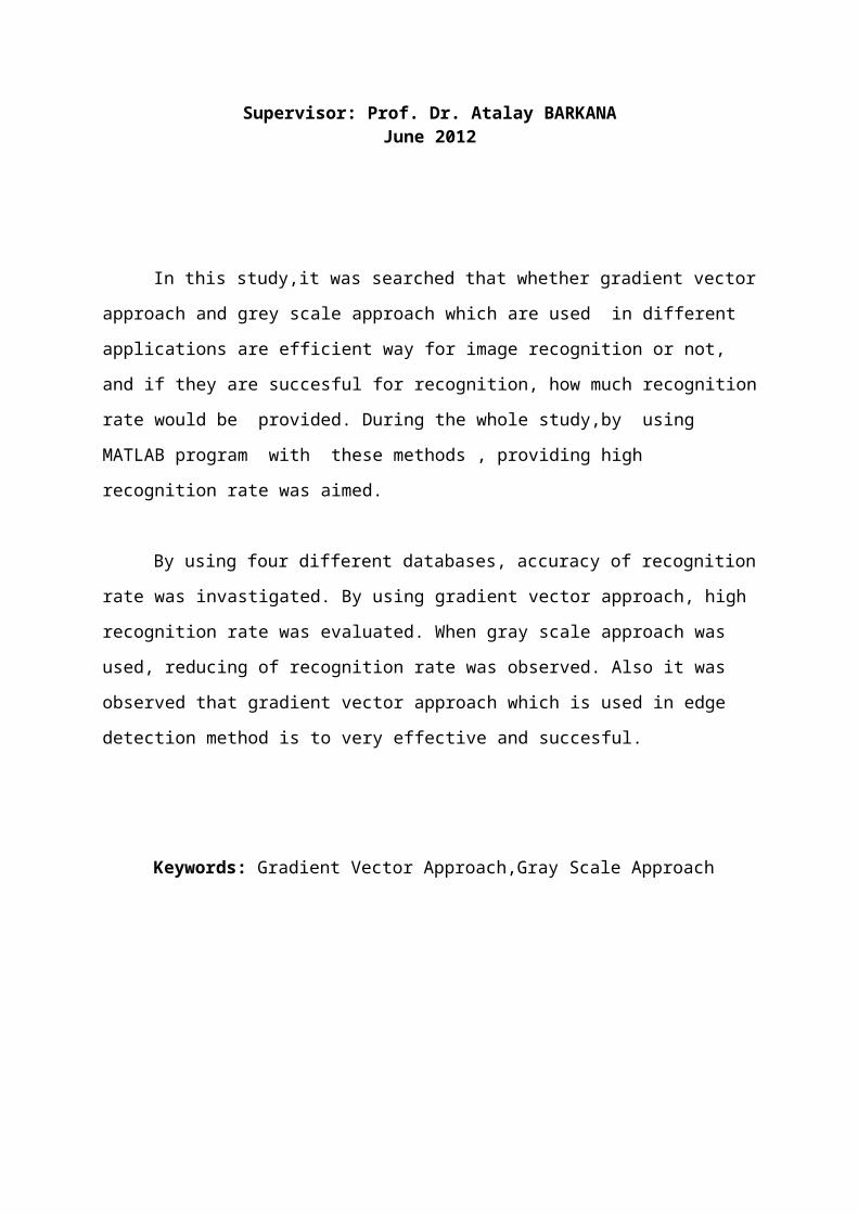
In this study,it was searched that whether gradient vector approach and grey scale
approach which are used in different applications are efficient way for image recognition or
not, and if they are succesful for recognition, how much recognition rate would be provided.
During the whole study,by using MATLAB program with these methods , providing high
recognition rate was aimed.
By using four different databases, accuracy of recognition rate was invastigated. By
using gradient vector approach, high recognition rate was evaluated. When gray scale
approach was used, reducing of recognition rate was observed. Also it was observed that
gradient vector approach which is used in edge detection method is to very effective and
succesful.
Keywords: Gradient Vector Approach,Gray Scale Approach
ÖZET
Lisans Tezi
Fonksiyonlar Arası Uzaklık
Eşref BOĞAR
ANADOLU ÜNİVERSİTESİMühendislik Mimarlık Fakültesi
Elektrik Elektronik Mühendisliği Bölümü
Danışman: Prof.Dr. Atalay BARKANAHaziran 2012
Bu projede,farklı uygulamalarda kullanılan gradyent vektör yaklaşımı ve gri tonlama
yaklaşımının görüntü tanımada da başarılı olup olmayacağını,başarılı olursa da ne kadar
tanıma oranı elde edileceği araştırılmıştır.Çalışma süresince MATLAB programı kullanılarak
bu yöntemlerle yüksek tanıma oranı sağlanması amaçlanmıştır.
4 farklı veri tabanı kullanılarak tanıma oranlarının tutarlılığı incelenmiştir. Gradyent
vektör yaklaşımı kullanılarak yüksek tanıma oranları elde edilmiştir.Gri tonlama yaklaşımı
kullanıldığında tanıma oranlarının düştüğü gözlemlenmiştir. Kenar bulma yönteminde
kullanılan gradyent vektör yaklaşımının ise çok başarılı ve etkili olduğunu gözlenmiştir.
Anahtar Kelimeler: Gradyent Vektör Yaklaşımı, Gri Tonlama Yaklaşımı
ACKNOWLEDGEMENT

First of all, I would like to thank to my supervisor of this project, Prof. Dr. Atalay
BARKANA for sharing his knowledge and experience with me. He inspired and informed me
greatly to work on this project.
Besides, I would like to thank to Mehmet KOÇ and my friends for supporting me
while working on the project.
CONTENTS

Pages
ABSTRACT………………………………………………..………………………i
ÖZET………………………………………….................................................ii
ACKNOWLEDGEMENT………………………………………………………..iii
CONTENTS................................................................................................iv
LIST OF FIGURES………………………………………………………………vi
LIST OF TABLES……………………………………………………………….vii
1.INTRODUCTION……………………………………………………………. 1 2.THEORITICAL BACKGROUND................................................................. 3
3.SOFTWARE OF PROJECT…………………………………………………..4
3.1. Recognition by Dividing to Norm of Gradient……………………………….5
3.1.1. Determining Images for Training Set and Test Set………………….5
3.1.2. Finding Gradient Values and Their Norm Values for Images……....6
3.1.3.Making Dot Product of Each Pixel at The Same Location…………..6
3.1.4.Summation of Scalar Multiplied Pixel……………………………….7
3.1.5. Determining Which Image Belongs to Which Classes ……………..7
3.1.5.a. Finding From The Highest Value of Each Classes………………..7
3.1.5.b.By Making Summation of The Values From Each Class………….9
3.1.6. Computıng Whıch Images Belong to Whıch Classes………………10
3.1.7. Evaluating Recognition Rate………………………………………..12
3.2. Recognition with Gradient Vector Values…………………………………..12
3.2.1 Determining Which Image Belongs to Which Class………………..12
3.2.1.a. Finding From the Highest Value of Each Class………………....12
3.2.1.b.By Making Summation of The Values From Each Class…………13
3.2.2. Computing Which Images Belong to Which Class…………………13
3.2.3 Evaluating Recognition Rate………………………………………...15
3.3. Recognition by Taking Substraction of Each Pixel………………………...15
3.3.1.Subtraction of Two Images at The Same Location………………….15
3.3.2.Determining Which Image Belongs to Which Class………………..15
3.3.2.a.Finding from The Lowest Value of Each Class………………….15
3.3.2.b.By Making Summation of the Values from Each Class…………16
3.3.3.Computing Which Images Belong to Which Class………………...17

3.3.4.Evaluating Recognition Rate…………………………………….....18
3.4. Method of Edge Detection…………………………………………………..19
3.4.1. Choosing a Image Whose Edge Would be Found out…………….19
3.4.2-Having 2D-Derivatıon of Each Images…………………………….19
3.4.3- Plotting Derivation of Each Values onto X and Y Axis…………..19
3.4.4.Finding Treshold Value……………………………………………..21
3.4.5. Making‘OR’Operation to the Values in The Direction of X and Y .21
3.4.6. Plotting the Graphics Image of each Images……………………….23
4.EXPERIMENTAL RESULTS……………………………………………….24
5.CONCLUSION………………………………………………………………..26
6.REFERENCES………………………………………………………………..27
7.APPENDIX……………………………………………………………………28
7.1.Appendix A…………………………………………………………………..28
7.2.Appendix B…………………………………………………………………..30
7.3 Appendix C…………………………………………………………………..32
LIST OF FIGURES
Figure 1 – Training set
Figure 2 – Test set
Figure 3 - An image for edge detection
Figure 4 - Derivation on the y-axis
Figure 5 - Original image
Figure 6 - Edge detection on the y-axis
Figure 7 - Edge detection on the x-axis
Figure 8 - Edge detection of image
Figure 9 - Edge detection
LIST OF TABLES
Table 1-Determination values by using the highest value
Table 2- Determination values by making summation
Table 3-Classes of images in the test set 1
Table 4- Determination values with gradient vector by using the highest value

Table 5- Determination values with gradient vector by making summation
Table 6- Classes of images in the test set 2
Table 7- Determination values with gradient vector by using the lowest value
Table 8- Determination values with gradient vector by making subtraction
Table 9-Classes of images in the test set 3
ABSTRACT
Graduation Project
Distance Between Function
Eşref BOĞAR
ANADOLU UNIVERSITYFaculty of Engineering and Architecture
Department of Electrical and Electronics Engineering
Supervisor: Prof. Dr. Atalay BARKANAJune 2012
In this study,it was searched that whether gradient vector approach and grey scale
approach which are used in different applications are efficient way for image recognition or
not, and if they are succesful for recognition, how much recognition rate would be provided.
During the whole study,by using MATLAB program with these methods , providing high
recognition rate was aimed.
By using four different databases, accuracy of recognition rate was invastigated. By
using gradient vector approach, high recognition rate was evaluated. When gray scale
approach was used, reducing of recognition rate was observed. Also it was observed that
gradient vector approach which is used in edge detection method is to very effective and
succesful.
Keywords: Gradient Vector Approach,Gray Scale Approach

ÖZET
Lisans Tezi
Fonksiyonlar Arası Uzaklık
Eşref BOĞAR
ANADOLU ÜNİVERSİTESİMühendislik Mimarlık Fakültesi
Elektrik Elektronik Mühendisliği Bölümü
Danışman: Prof.Dr. Atalay BARKANAHaziran 2012
Bu projede,farklı uygulamalarda kullanılan gradyent vektör yaklaşımı ve gri tonlama
yaklaşımının görüntü tanımada da başarılı olup olmayacağını,başarılı olursa da ne kadar
tanıma oranı elde edileceği araştırılmıştır.Çalışma süresince MATLAB programı kullanılarak
bu yöntemlerle yüksek tanıma oranı sağlanması amaçlanmıştır.
4 farklı veri tabanı kullanılarak tanıma oranlarının tutarlılığı incelenmiştir. Gradyent
vektör yaklaşımı kullanılarak yüksek tanıma oranları elde edilmiştir.Gri tonlama yaklaşımı
kullanıldığında tanıma oranlarının düştüğü gözlemlenmiştir. Kenar bulma yönteminde
kullanılan gradyent vektör yaklaşımının ise çok başarılı ve etkili olduğunu gözlenmiştir.
Anahtar Kelimeler: Gradyent Vektör Yaklaşımı, Gri Tonlama Yaklaşımı
ACKNOWLEDGEMENT

First of all, I would like to thank to my supervisor of this project, Prof. Dr. Atalay
BARKANA for sharing his knowledge and experience with me. He inspired and informed me
greatly to work on this project.
Besides, I would like to thank to Mehmet KOÇ and my friends for supporting me
while working on the project.
CONTENTS

Pages
ABSTRACT………………………………………………..………………………i
ÖZET………………………………………….................................................ii
ACKNOWLEDGEMENT………………………………………………………..iii
CONTENTS................................................................................................iv
LIST OF FIGURES………………………………………………………………vi
LIST OF TABLES……………………………………………………………….vii
1.INTRODUCTION……………………………………………………………. 1 2.THEORITICAL BACKGROUND................................................................. 3
3.SOFTWARE OF PROJECT…………………………………………………..4
3.1. Recognition by Dividing to Norm of Gradient……………………………….5
3.1.1. Determining Images for Training Set and Test Set………………….5
3.1.2. Finding Gradient Values and Their Norm Values for Images……....6
3.1.3.Making Dot Product of Each Pixel at The Same Location…………..6
3.1.4.Summation of Scalar Multiplied Pixel……………………………….7
3.1.5. Determining Which Image Belongs to Which Classes ……………..7
3.1.5.a. Finding From The Highest Value of Each Classes………………..7
3.1.5.b.By Making Summation of The Values From Each Class………….9
3.1.6. Computıng Whıch Images Belong to Whıch Classes………………10
3.1.7. Evaluating Recognition Rate………………………………………..12
3.2. Recognition with Gradient Vector Values…………………………………..12
3.2.1 Determining Which Image Belongs to Which Class………………..12
3.2.1.a. Finding From the Highest Value of Each Class………………....12
3.2.1.b.By Making Summation of The Values From Each Class…………13
3.2.2. Computing Which Images Belong to Which Class…………………13
3.2.3 Evaluating Recognition Rate………………………………………...15
3.3. Recognition by Taking Substraction of Each Pixel………………………...15
3.3.1.Subtraction of Two Images at The Same Location………………….15
3.3.2.Determining Which Image Belongs to Which Class………………..15
3.3.2.a.Finding from The Lowest Value of Each Class………………….15
3.3.2.b.By Making Summation of the Values from Each Class…………16
3.3.3.Computing Which Images Belong to Which Class………………...17
3.3.4.Evaluating Recognition Rate…………………………………….....18
3.4. Method of Edge Detection…………………………………………………..19
3.4.1. Choosing a Image Whose Edge Would be Found out…………….19
3.4.2-Having 2D-Derivatıon of Each Images…………………………….19
3.4.3- Plotting Derivation of Each Values onto X and Y Axis…………..19
3.4.4.Finding Treshold Value……………………………………………..21
3.4.5. Making‘OR’Operation to the Values in The Direction of X and Y .21
3.4.6. Plotting the Graphics Image of each Images……………………….23
4.EXPERIMENTAL RESULTS……………………………………………….24
5.CONCLUSION………………………………………………………………..26
6.REFERENCES………………………………………………………………..27
7.APPENDIX……………………………………………………………………28
7.1.Appendix A…………………………………………………………………..28
7.2.Appendix B…………………………………………………………………..30
7.3 Appendix C…………………………………………………………………..32
LIST OF FIGURES
Figure 1 – Training set
Figure 2 – Test set
Figure 3 - An image for edge detection

Figure 4 - Derivation on the y-axis
Figure 5 - Original image
Figure 6 - Edge detection on the y-axis
Figure 7 - Edge detection on the x-axis
Figure 8 - Edge detection of image
Figure 9 - Edge detection
LIST OF TABLES
Table 1-Determination values by using the highest value
Table 2- Determination values by making summation
Table 3-Classes of images in the test set 1
Table 4- Determination values with gradient vector by using the highest value

Table 5- Determination values with gradient vector by making summation
Table 6- Classes of images in the test set 2
Table 7- Determination values with gradient vector by using the lowest value
Table 8- Determination values with gradient vector by making subtraction
Table 9-Classes of images in the test set 3
1.INTRODUCTIONThe gradient of a function is a vector that points in the direction in which the function
changes most rapidly and has a magnitude equal to the rate of change of the function in that
direction. It is the natural three-dimensional generalization of the derivative with respect to a
single variable. In Cartesian coordinates, the gradient of the function can be written:[1]
In Graduation Project, Distance Between Funtions with using gradient vectors and
gray scale approach are studied on MATLAB. By using four different databases, we could
have noticable consequences in order to compare results for each database which is shown
below:
AR : This database includes 50 classes and each one has 14 different images . In this
database, eyes of the each person are stable but their mimics are different
FERET: This database consists 200 classes and each one has 2 different images. In
this database, both eyes of the each person and their mimics are different.
ORL: This database includes 40 classes and each one has 10 different images. In this
database, both eyes of the each person and their mimics are different. In addition direction of
each images are different.
YALE: This database includes 50 classes and each one 14 different images. In this
database, eyes of the each people are stable but their mimics are different. Also in this
database, different types of artificial illuminiation is used.
Half of the each class of databases were used as a test set and other half were used as
a training set.
In this graduation Project Distance Between Functions, gradient vector has been used
in order to find the recognation rates of each databases and also it used for observing whether
it finds the edge or not.
Additionaly, images which damage the recognition rate were investigated.
As a result of all these studies, using gradient vector approches in patern recognition
is very useful way in order to get the efficient recognition rates is reached with some
experimental proof.

2.THEORETICAL BACKGROUNDEdge detection is the process of localizing pixel intensity transitions. The edge
detection has been used by object recognition, target tracking, segmentation, and etc.
Therefore, the edge detection is one of the most important parts of image processing.
There mainly exist several edge detection methods. These methods have been proposed
for detecting transitions in images. Early methods determined the best gradient operator
to detect sharp intensity variations . Commonly used method for detecting edges is to
apply derivative operators on images. Derivative based approaches can be categorized
into two groups, namely first and second order derivative methods. First order derivative
based techniques depend on computing the gradient several directions and combining
the result of each gradient. The value of the gradient magnitude and orientation is
estimated using two differentiation masks . In this work, Gradient vector which is an edge
detection method is considered.[2]
Some formulas which we used in gradient vector approach are in the following:

3.SOFTWARE OF PROJECTIn this graduation Project some applications under the subject of Distance Between
Functions were made. These applications and their steps are shown below
Recognition by dividing to norm of gradient
Determining images for training set and test set
Finding gradient values and their norms values for images
Making dot product of each pixel at the same location
Summation of scalar multiplied pixels
Determining which image belongs to which class
A)Finding from the highest value of each class
B) By making summation of the values from each class
Computing which images belong to which class
Evaluating recognition rate
Recognition with gradient vector values
Determining images for training set and test set
Making dot product of each pixel at the same location
Summation of scalar multiplied pixels
Determining which image belongs to which class
A)Finding from the highest value of each class
B) By making summation of the values from each class
Computing which images belong to which class
Evaluating recognition rate
Recognition by taking substraction of each pixel
Determining images for training set and test set
Subtraction of two images at the same location
Determining which image belongs to which class
A)Finding from the lowest value of each class
B) By making summation of the values from each class
Computing which images belong to which class
Evaluating recognition rate

Method of edge detection
Choosing a image whose edge would be found out
Having 2D derivation of each images
Plotting derivation of each value onto x and y axis
Finding treshold value
Making ‘or’ operation to the values in the direction of x and y
Plotting the graphics image
3.1. Recognition by Dividing to Norm of Gradient
When the gradient vector’magnitude equals 1, the steps that are applied in the
following;
3.1.1. Determining Images for Training Set and Test Set
Half of the images of each class were produced as training set. Other half of images of
each class were produced as test set.
Figure 1- Training set
Figure 2- Test set
3.1.2. Finding Gradient Values and Their Norm Values for Images

2D -Gradients of the both training set and test set are calculated for each pixel and
their norm values are calculated.
Matlab code:
for m=2:satir-1 %cercevenin işlem dışı olması için for n=2:sutun-1 %for training set a2(m-1,n-1)=r(m,n+1)-r(m,n); b2(m-1,n-1)=r(m+1,n)-r(m,n); c2(m-1,n-1)=sqrt(a2(m-1,n-1)*a2(m-1,n-1)+b2(m-1,n-1)*b2(m-1,n-1)); %for test set a1(m-1,n-1)=t(m,n+1)-t(m,n); b1(m-1,n-1)=t(m+1,n)-t(m,n); c1(m-1,n-1)=sqrt(a1(m-1,n-1)*a1(m-1,n-1)+b1(m-1,n-1)*b1(m-1,n-1)); end end
3.1.3.Making Dot Product of Each Pixel at The Same Location
In here, we have used dot product of each pixel which are training set and test set at
the same location.
Matlab code:
for w=2:satir-1 for s=2:sutun-1 if c2(w-1,s-1)==0 || c1(w-1,s-1)==0m(w-1,s-1)=1; else m(w-1,s-1)=(a1(w-1,s-1).*a2(w-1,s-1))/(c2(w-1,s-1)*c1(w-1,s-1))+(b1(w-1,s-1).*b2(w-1,s-1))/(c2(w-1,s-1)*c1(w-1,s-1)); end end end
3.1.4.Summation of Scalar Multiplied Pixel
All values at the ecah pixel of image has been accumulated.
Matlab code:
toplam=sum(sum(m));3.1.5. Determining Which Image Belongs to Which Classes
Methods were investigated around which image belong to which class in details.
These methods are;
3.1.5.a. Finding From The Highest Value of Each Classes
Excepting the image to belong to the class in which has the highest value that we have
evaluated.
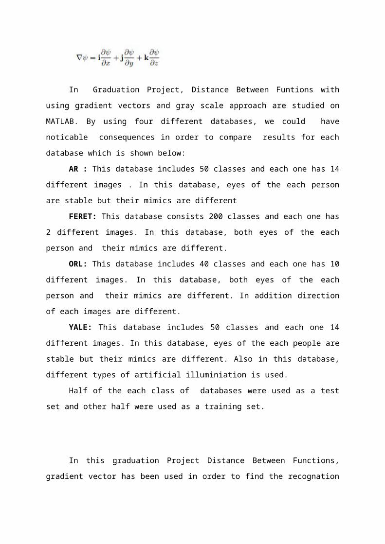
Table 1-Determination values by using the highest value
We could observe from table 1 the highest value is 6300,388 which belongs to class 1,
therefore we reached that the eighth image of the class 1 in training set belongs to directly to
class 1.
3.1.5.b.By Making Summation of The Values From Each Class
Excepting the image to belong to the class in which has the with highest value of
summation that we have evaluated.

Table 2- Determination values by making summation
As we are seeing from Table 2, after making summation and having the highest value
which is 317770,14 belongs to class-1.Consequently, we could observe that the eight image of
the class 1 in training set belongs to class 1.
3.1.6. Computıng Whıch Images Belong to Whıch Classes
Which images in the test set belong to which classes have been foun out and showed
on the table. According to the highest value.

Table 3-Classes of images in the test set
3.1.7. Evaluating Recognition Rate
Recognition rate was accumulated by checking the images at the test set.

Matlab code:
to=(count4/((resim*sınıf))/2)*100
3.2. Recognition with Gradient Vector Values
Determining images for training set and test set, making dot product of each pixel at
the same location, summation of scalar multiplied pixels, computing which images belong to
which class, these steps at the Recognition By Dividing to Norm of Gradient has been
repeated again at this part.
3.2.1 Determining Which Image Belongs to Which Class
Two methods which shown below were applied with regarding the gradient values.
3.2.1.a. Finding From the Highest Value of Each Class
Excepting the image to belong to the class in which has the highest value that we have
evaluated.
Table 4- Determination values with gradient vector by using the highest value
Classes which are from 1 to 20 were investigated and the values at the other classes
were observed less than 2029882
We could observe from table 1the highest value is 2029882 which belongs to class 1,
therefore we reached that the eighth image of the class 1 in training set belongs to directlyto
class 1.
3.2.1.b.By Making Summation of The Values From Each Class
Excepting the image to belong to the class in which has the with highest value of
summation that we have evaluated.

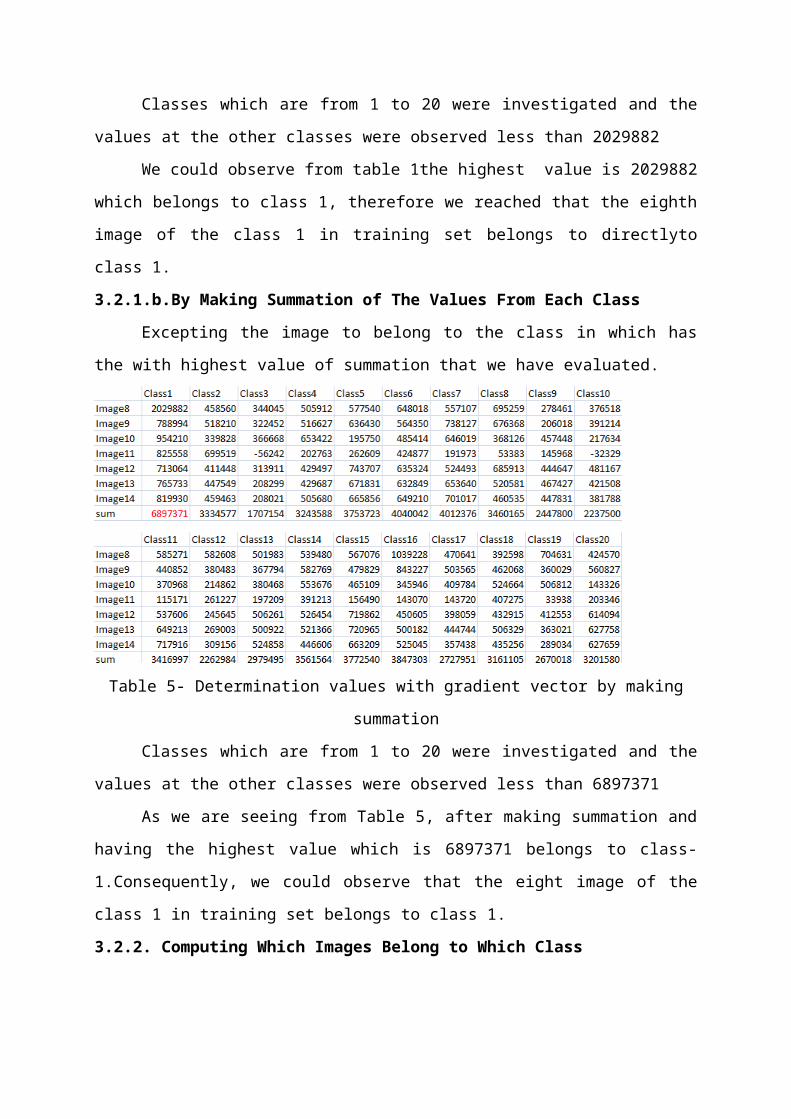
Table 5- Determination values with gradient vector by making summation
Classes which are from 1 to 20 were investigated and the values at the other classes
were observed less than 6897371
As we are seeing from Table 5, after making summation and having the highest value
which is 6897371 belongs to class-1.Consequently, we could observe that the eight image of
the class 1 in training set belongs to class 1.
3.2.2. Computing Which Images Belong to Which Class
Which images in the test set belong to which classes have been foun out and showed
on the table. According to the highest value.
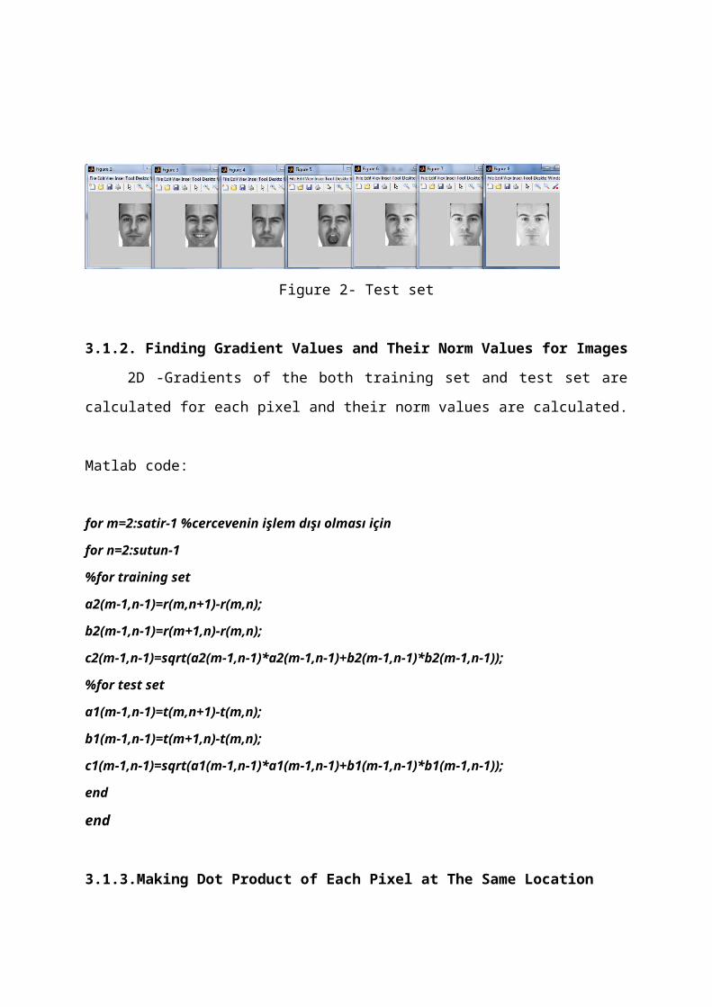
Table 6- Classes of images in the test set 2
3.2.3 Evaluating Recognition Rate
Recognition rate was accumulated by checking the images at the test set.
Matlab code:
to=(count/((resim*sınıf))/2)*100
3.3. Recognition by Taking Substraction of Each Pixel
Determining images for training set and test set , this step at the Recognition By Dividing
to Norm of Gradient has been repeated again at this part.
3.3.1.Subtraction of Two Images at The Same Location
Matlab code:
for w=2:satir-1 for s=2:sutun-1 x=abs(t(w,s)-r(w,s)); m(w-1,s-1)=x; end end
3.3.2.Determining Which Image Belongs to Which Class
Two methods which shown below were applied with regarding the gray scale values.

3.3.2.a.Finding from The Lowest Value of Each Class
Excepting the image to belong to the class in which has the lowest value that we have
evaluated.
Table 7- Determination values with gradient vector by using the lowest value
We could observe from table 1 the lowest value is 91946 which belongs to class 1,
therefore we reached that the eighth image of the class 1 in training set belongs to directly to
class 1.
3.3.2.b.By Making Summation of the Values from Each Class

Excepting the image to belong to the class in which has the with lowest value of
summation that we have evaluated.
Table 8- Determination values with gradient vector by making subtraction
Classes which are from 1 to 20 were investigated and the values at the other classes
were observed more than 1768339.
As we are seeing from Table 8, after making subtraction and having the lowest value
which is1768339 belongs to class-1.Consequently, we could observe that the eight image of
the class 1 in training set belongs to class 1.
3.3.3.Computing Which Images Belong to Which Class
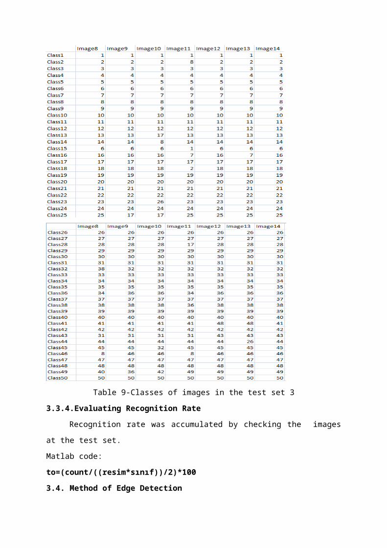
Which images in the test set belong to which classes have been foun out and showed
on the table. According to the lowest value:

Table 9-Classes of images in the test set 3
3.3.4.Evaluating Recognition Rate
Recognition rate was accumulated by checking the images at the test set.
Matlab code:
to=(count/((resim*sınıf))/2)*100
3.4. Method of Edge Detection
3.4.1- Choosing a Image Whose Edge Would be Found out

Figure 3-An image for edge detection
Matlab code:
a=V{11,1};t=uint8(a);[satir sutun]=size(t); figureimshow(t)
3.4.2-Having 2D-Derivatıon of Each Images
Matlab code:
for i=1:satir-1 for j=1:sutun-1 str(i,j)=(a(i+1,j)-a(i,j)); %x ekseni üzerinde türev stn(i,j)=(a(i,j+1)-a(i,j)); %y ekseni üzerinde türev endend
3.4.3- Plotting Derivation of Each Values onto X and Y Axis
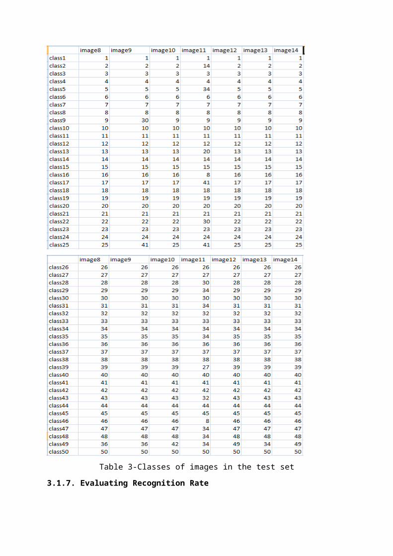
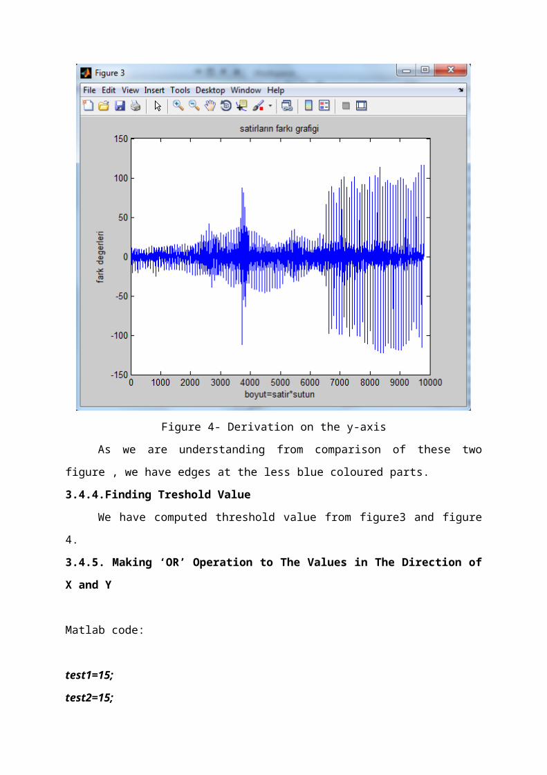
Figure-4 Derivation on the y-axis
In figure 3, derivated values on the direction of y have been plotted.
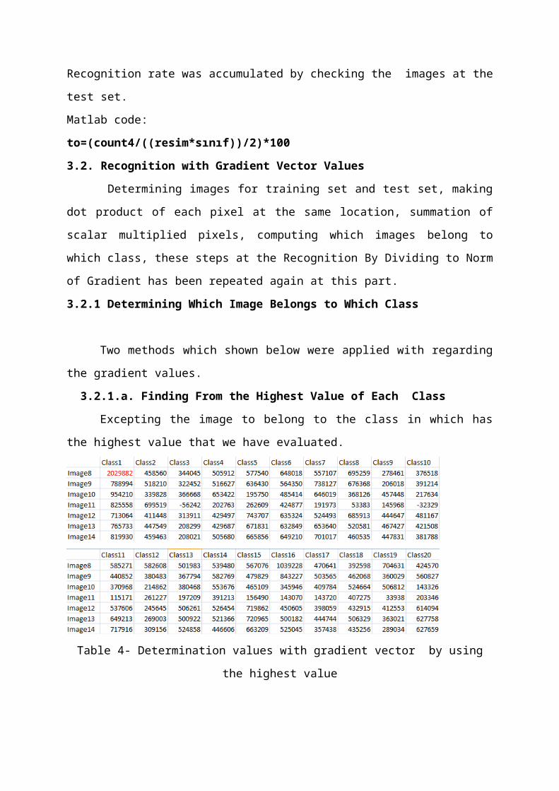
Figure 4- Derivation on the y-axis
As we are understanding from comparison of these two figure , we have edges at the
less blue coloured parts.
3.4.4.Finding Treshold Value
We have computed threshold value from figure3 and figure 4.
3.4.5. Making ‘OR’ Operation to The Values in The Direction of X and Y
Matlab code:
test1=15;test2=15;test3=15;test4=15;for i=1:satir-1 for j=1:sutun-1
b(i,j)=str(i,j); c(i,j)=stn(i,j); if str(i,j)>=test1 b(i,j)=1; end if str(i,j)<=-test2 b(i,j)=1; end if str(i,j)<test1 && str(i,j)>-test2 b(i,j)=0; end if stn(i,j)>=test3 c(i,j)=1; end if stn(i,j)<=-test4 c(i,j)=1; end if stn(i,j)<test3 && stn(i,j)>-test4 c(i,j)=0; end d(i,j)=b(i,j)+c(i,j); if d(i,j)==2 d(i,j)=1; end endend
3.4.6. Plotting the Graphics Image of each Images
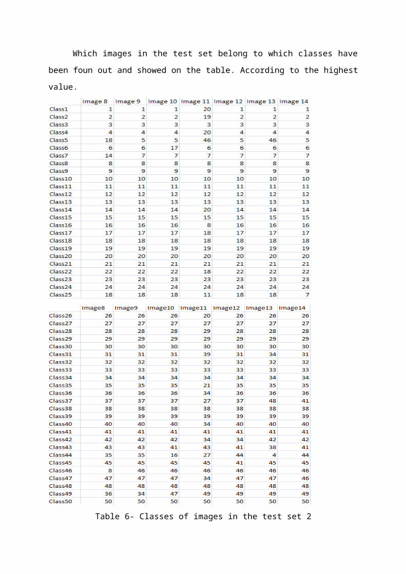
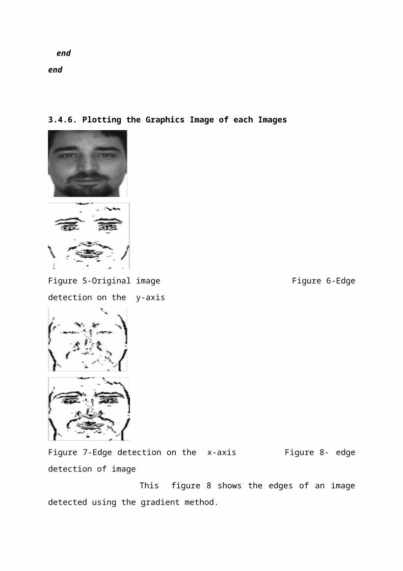
Figure 5-Original image Figure 6-Edge detection on the y-axis
Figure 7-Edge detection on the x-axis Figure 8- edge detection of image
This figure 8 shows the edges of an image detected using the gradient method.
4.EXPERIMENTAL RESULTSSome applications by providing the derivation of gradient vector and gray scale
throuh the x and y axis were made under the subjects of recognition by dividing to norm
of gradient, recognition with gradient vector values, recognition by taking substraction of
each pixel,method of edge detection.
Recognition rates were found by using four different databases in these applications.
Recognition by dividing to norm of gradient
By finding from the highest value ;
AR 97.7143%
ORL 53%

FERET 73%
YALE 92%
By making summation of the values from;
AR 93.4286%
ORL 63%
FERET 73%
YALE 89.3333%
Recognition with gradient vector values By finding from the highest value ;
AR 86.5714%
ORL 54.5%
FERET 49.5%
YALE 85.56%
By making summation of the values from;
AR 79.1429%
ORL 46%
FERET 49.5%
YALE 88,89%
Recognition by taking substraction of each pixel
By finding from the lowest value ; AR 90.2857%
ORL 94%
FERET 92%
By making summation of the values from;
AR 56%
ORL 86.5%
FERET 92%
Method of edge detection

Figure 9-Edge detection
5.CONCLUSIONSome metods which are Gradient Vector Approach and Gray Scale Approach were
used under the subject of Distance between Functions. By using four different databases with
these methods on some applications, accuracy of results were analiazed. Our aim was either
gradient vector approach or gray scale approch is effective to provide the maximum
recognition rate.
In gradient vector approach, we studied with theree different metods. Our first method
is Recognition by dividing gradient vector to its norm.The best recognition rates were
evaluated by using this first method. Our second method is Recognition with gradient vector
values. Opposite to the first method, less recognition rate was observed by using this method.
Our last method is Edge Detection which finds the edge of the image. By using this process,
very effective consequences were provided. Additionally during the usage of this method, by
studying on maximum and summed values of each class, finding the maximum recognition
rate was aimed. The maximum recognition rate is provided , when we made an application to
the maximum value.
When we used Gray scale approach , we also reached maximum recognition rates. By
applying this method to the minimum values, maximum recognition rate was observed.
As a result, we have observed that , by usuing gradient vector approach and gray scale
approach, we could provide an efficient recognition and maximum recognition rates
effectively. Also it is understood that these two methods could be very successful ways for
pattern recognition too.

6.REFERENCES[1] http://www.physics.rutgers.edu/ugrad/494/bookr03D.pdf
[2] http://www.figes.com.tr/matlab/teknik-makaleler/eaybar_tam_metin.pdf
7.APPENDIX7.1.Appendix A
sinif=50;resim=14;satir=115;sutun=87;class=1;count=0;sat=1;sut=1;
k=0;w3=1;for y=1:siniffor x=resim/2+1:resim a=V{y,x}; t=double(a); %double a dönüştürme for i=1:sinif for j=1:resim/2 %tüm resimler b=V{i,j}; r=double(b); %double a dönüştürme for m=2:satir-1 for n=2:sutun-1 %2.resim için a2(m-1,n-1)=r(m,n+1)-r(m,n); %y ye göre türev b2(m-1,n-1)=r(m+1,n)-r(m,n); %x e göre türev c2(m-1,n-1)=sqrt(a2(m-1,n-1)*a2(m-1,n-1)+b2(m-1,n-1)*b2(m-1,n-1)); %1.resim için a1(m-1,n-1)=t(m,n+1)-t(m,n); %y ye göre türev b1(m-1,n-1)=t(m+1,n)-t(m,n); %x e göre türev c1(m-1,n-1)=sqrt(a1(m-1,n-1)*a1(m-1,n-1)+b1(m-1,n-1)*b1(m-1,n-1)); end end %2 resimde karsı gelen piksellerin skaler carpımı for w=2:satir-1 for s=2:sutun-1 if c2(w-1,s-1)==0 || c1(w-1,s-1)==0 m(w-1,s-1)=1; else m(w-1,s-1)=(a1(w-1,s-1).*a2(w-1,s-1))/(c2(w-1,s-1)*c1(w-1,s-1))+(b1(w-1,s-1).*b2(w-1,s-1))/(c2(w-1,s-1)*c1(w-1,s-1)); end end end toplam=sum(sum(m)); %14x50 lik sonucları yazdırma if k<resim/2 sonuc1(sat,sut)=toplam; k=k+1; sat=sat+1; else

sut=sut+1; sat=1; sonuc1(sat,sut)=toplam; k=1; sat=sat+1; end end end%en büyük değer methoduyla yapmak için en buyuk degerfor e=1:sinif rrr(:,e)=max(sonuc1(:,e));endf=sort(rrr);for e1=1:sinif if rrr(1,e1)==f(1,sinif); %hangi sınıfa ait olduğunu bulma klm{w3}=e1;%sınıfları arraye atama w3=w3+1; endend sat=1;sut=1;k=0; endend%Tanıma oranını bulmau=1;h=0;count4=0;for as=1:resim*sinif/2 if h<resim/2 h=h+1; if klm{as}==u count4=count4+1; end else u=u+1; if klm{as}==u count4=count4+1; end h=1; endendto=(count4/(sinif*resim/2))*100
7.2.Appendix B
sinif=50;resim=14;

satir=115;sutun=87;class=1;count=0;sat=1;sut=1;k=0;w3=1;for y=1:siniffor x=resim/2+1:resim a=V{y,x}; t=double(a); %double a dönüştürme for i=1:sinif for j=1:resim/2 %tüm resimler b=V{i,j}; r=double(b); %double a dönüştürme for m=2:satir-1 for n=2:sutun-1 a2(m-1,n-1)=r(m,n+1)-r(m,n); %y ye göre türev b2(m-1,n-1)=r(m+1,n)-r(m,n); %x e göre türev a1(m-1,n-1)=t(m,n+1)-t(m,n); %y ye göre türev b1(m-1,n-1)=t(m+1,n)-t(m,n); %x e göre türev end end %2 resimde karsı gelen piksellerin skaler carpımı for w=2:satir-1 for s=2:sutun-1 m(w-1,s-1)=(a1(w-1,s-1).*a2(w-1,s-1))+(b1(w-1,s-1).*b2(w-1,s-1)); end end toplam=sum(sum(m)); %14x50 lik sonucları yazdırma if k<resim/2 sonuc1(sat,sut)=toplam; k=k+1; sat=sat+1; else
sut=sut+1; sat=1; sonuc1(sat,sut)=toplam; k=1; sat=sat+1; end end end%en büyük değer methoduyla yapmak için en buyuk degerfor e=1:sinif rrr(:,e)=max(sonuc1(:,e));endf=sort(rrr);for e1=1:sinif if rrr(1,e1)==f(1,sinif); %hangi sınıfa ait olduğunu bulma klm{w3}=e1;%sınıfları arraye atama w3=w3+1; endend sat=1;sut=1;k=0; endend%Tanıma oranını bulmau=1;h=0;count4=0;for as=1:resim*sinif/2 if h<resim/2 h=h+1; if klm{as}==u count4=count4+1; end else u=u+1; if klm{as}==u count4=count4+1; end h=1; endendto=(count4/(sinif*resim/2))*100
7.3.Appendix C
sinif=50;resim=14;

satir=115;sutun=87;class=1;count=0;sat=1;sut=1;k=0;w3=1;for y=1:1for x=8:8 a=V{y,x}; t=double(a); %double a dönüştürme for i=1:sinif for j=1:resim/2 %tüm resimler b=V{i,j}; r=double(b); %double a dönüştürme for w=2:satir-1 for s=2:sutun-1 x=abs(t(w,s)-r(w,s)); m(w-1,s-1)=x; end end toplam=sum(sum(m)); %14x50 lik sonucları yazdırma if k<resim/2 sonuc1(sat,sut)=toplam; k=k+1; sat=sat+1; else sut=sut+1; sat=1; sonuc1(sat,sut)=toplam; k=1; sat=sat+1; end endendfor e=1:sinif rrr(:,e)=min(sonuc1(:,e));end
f=sort(rrr);for e1=1:sinif if rrr(1,e1)==f(1,1); klm{w3}=e1; w3=w3+1; endend sat=1;sut=1;k=0; endendu=1;h=0;count4=0;for as=1:resim*sinif/2 if h<resim/2 h=h+1; if klm{as}==u count4=count4+1; end else u=u+1; if klm{as}==u count4=count4+1; end h=1; endendto=(count4/(sinif*resim/2))*100