1

3X3 ROD BUNDLE INVESTIGATIONS, CFD SINGLE-PHASE NUM ERICAL SIMULATIONS

C. Lifante*, B. Krull*, Th. Frank*, R. Franz † and U. Hampel†

* ANSYS Germany GmbH, Staudenfeldweg 12, Otterfing, D-83624, Germany † Institut für Sicherheitsforschung,Helmholtz Zentrum Dresden-Rossendorf, POB 510 119,

Dresden, D-01314, Germany

Conxita.Lifante@ansys.com

Abstract The aim of this work is to numerically investigate in detail a 3x3 rod bundle geometry. This geometry has been chosen to reproduce the ROFEX facility at HZDR, that it is just starting up. That facility has been constructed to develop a new multiphase technique and to provide future experimental information to validate boiling models in CFD codes. Therefore, a 3x3 rod bundle geometry was built in the facility, which can be representative of the real fuel assembly geometries in nuclear reactors. As a first stage the investigations here presented were conducted, where CFD single-phase simulations were performed. For the validation of the numerical results PIV measurements were used. The simulation domain consists of a horizontal inlet pipe entering in a chamber where the flow turns up to the main (vertical) pipe. The main purpose of this inlet chamber is to ensure a flow inlet into the rod bundle with as less as possible flow disturbances in this vertical arrangement of the bundle and with the given space restrictions of the laboratory. The main section of the rod bundle is 978 mm long, contains 3x3=9 rods and it is connected to another chamber and a horizontal outlet pipe. The main pipe diameter is 54 mm and the diameter of the rods is 10.2 mm. As working fluid p-cymene was chosen for the PIV measurements. Experiments had been carried out at normal temperature and pressure. Experiments and simulations were conducted for three different inlet volume flow rates: 1.24 l/s, 1.72 l/s and 2.14 l/s. Different geometry models were considered: the whole geometry or just the main vertical pipe where the rods are included. Both cases in turn were investigated with or without a grid spacer, that means in total four different configurations were considered. Best Practice guidelines were followed where possible and for this purpose two numerical grids were created using ANSYS ICEM CFD Hexa for each geometry model. A refinement factor of two in each coordinate direction has been applied for the regular mesh refinement of the hexahedral meshes. All meshes were constructing keeping in mind that they will be used in further boiling investigations. Steady state and transient simulations were conducted to investigate the character of the flow. Flow regions with strong streamline curvature show transient flow behavior, especially in the mixing zone of the upper outlet chamber. This effect was diminished in the lower inlet chamber due to the construction of a flow separator, which acts as a flow straightener. In addition an analysis of the influence of the turbulence modeling was performed, where the isotropic SST (Shear Stress Transport) model has been compared to the anisotropic BSL Reynolds Stress Model. Profiles of transient averaged velocity components were compared to the ensemble averaged experimental data from the PIV measurements at different elevations in the rod bundle and in different horizontal cross-sections through the rods and sub channels of the 3x3 bundle array. Hereby the analysis of secondary flows in the sub channels of the rod bundle is of particular interest.

2

1. INTRODUCTION

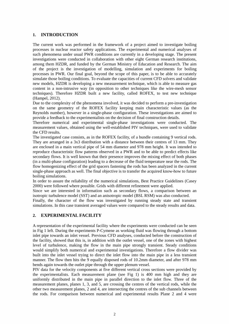
The current work was performed in the framework of a project aimed to investigate boiling processes in nuclear reactor safety applications. The experimental and numerical analyses of such phenomena under usual PWR conditions are currently in a developing stage. The present investigations were conducted in collaboration with other eight German research institutions, among them HZDR, and funded by the German Ministry of Education and Research. The aim of the project is the investigation of modelling, simulation and experiments for boiling processes in PWR. Our final goal, beyond the scope of this paper, is to be able to accurately simulate those boiling conditions. To evaluate the capacities of current CFD solvers and validate new models, HZDR is developing a new measurement technique, which is able to measure gas content in a non-intrusive way (in opposition to other techniques like the wire-mesh sensor techniques). Therefore HZDR built a new facility, called ROFEX, to test new technique (Hampel, 2012). Due to the complexity of the phenomena involved, it was decided to perform a pre-investigation on the same geometry of the ROFEX facility keeping main characteristic values (as the Reynolds number), however in a single-phase configuration. These investigations are aimed to provide a feedback to the experimentalists on the decision of final construction details. Therefore numerical and experimental single-phase investigations were conducted. The measurement values, obtained using the well-established PIV techniques, were used to validate the CFD results. The investigated case consists, as in the ROFEX facility, of a bundle containing 9 vertical rods. They are arranged in a 3x3 distribution with a distance between their centres of 13 mm. They are enclosed in a main vertical pipe of 54 mm diameter and 978 mm height. It was intended to reproduce characteristic flow patterns observed in a PWR and to be able to predict effects like secondary flows. It is well known that their presence improves the mixing effect of both phases (in a multi-phase configuration) leading to a decrease of the fluid temperature near the rods. The flow homogenizing effect of the grid spacers fastening the rods has been analyzed in the current single-phase approach as well. The final objective is to transfer the acquired know-how to future boiling simulations. In order to assure the reliability of the numerical simulations, Best Practice Guidelines (Casey 2000) were followed where possible. Grids with different refinement were applied. Since we are interested in information such as secondary flows, a comparison between an isotropic turbulence model (SST) and an anisotropic model (BSL RSM) was also conducted. Finally, the character of the flow was investigated by running steady state and transient simulations. In this case transient averaged values were compared to the steady results and data. 2. EXPERIMENTAL FACILITY A representation of the experimental facility where the experiments were conducted can be seen in Fig 1 left. During the experiments P-Cymene as working fluid was flowing through a bottom inlet pipe towards an inlet vessel. Previous CFD analyses, conducted before the construction of the facility, showed that this is, in addition with the outlet vessel, one of the zones with highest level of turbulence, making the flow in the main pipe strongly transient. Steady conditions would simplify both numerical and experimental investigations. Therefore a flow divider was built into the inlet vessel trying to direct the inlet flow into the main pipe in a less transient manner. The flow then hits the 9 equally disposed rods of 10.2mm diameter, and after 978 mm bends again towards the outlet pipe through the upper plenum vessel. PIV data for the velocity components at five different vertical cross sections were provided by the experimentalists. Each measurement plane (see Fig 1) is 400 mm high and they are uniformly distributed in the main pipe in parallel direction to the inlet flow. Three of the measurement planes, planes 1, 3, and 5, are crossing the centres of the vertical rods, while the other two measurement planes, 2 and 4, are intersecting the centres of the sub channels between the rods. For comparison between numerical and experimental results Plane 2 and 4 were

3

chosen (see Fig 1). Due to their intersection of the gaps between the rods and sub channels centres, planes 2 and 4 provide the most experimental information for this CFD model validation exercise. Experiments were conducted for three different inlet volume flows: 1.20 l/s; 1.70 l/s and 2.14 l/s, which correspond to 1.732 m/s; 2.454 m/s and 3.089 m/s inlet velocity respectively. Flow was kept isothermal at 28 C under 1 bar pressure. The selection of P-Cymene as working fluid was due to its optical properties. This fluid has matching refractive index with the glass walls of the geometry. Under these conditions it has the following properties: a density of 850.79 kg/m3; a dynamic viscosity of 0.761 x 10-3 kg/ms and a molar mass of 134.2 g/mol, which are about 85% of the water properties. The measurement error in axial direction was evaluated by the experimentalists to be 6 %. Further details regarding the measurements techniques and the experimental facility can be found in (Dominguez-Ontiveros, 2012).

Fig 1: Left: Representation of the experimental facility. Right: Location of the measurement

planes and elevations chosen for comparison.

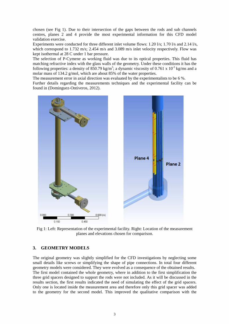
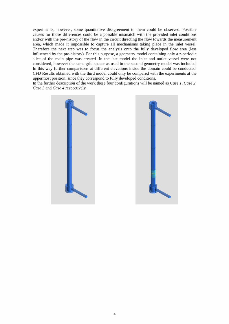
3. GEOMETRY MODELS The original geometry was slightly simplified for the CFD investigations by neglecting some small details like screws or simplifying the shape of pipe connections. In total four different geometry models were considered. They were evolved as a consequence of the obtained results. The first model contained the whole geometry, where in addition to the first simplification the three grid spacers designed to support the rods were not included. As it will be discussed in the results section, the first results indicated the need of simulating the effect of the grid spacers. Only one is located inside the measurement area and therefore only this grid spacer was added to the geometry for the second model. This improved the qualitative comparison with the

4

experiments, however, some quantitative disagreement to them could be observed. Possible causes for those differences could be a possible mismatch with the provided inlet conditions and/or with the pre-history of the flow in the circuit directing the flow towards the measurement area, which made it impossible to capture all mechanisms taking place in the inlet vessel. Therefore the next step was to focus the analysis onto the fully developed flow area (less influenced by the pre-history). For this purpose, a geometry model containing only a z-periodic slice of the main pipe was created. In the last model the inlet and outlet vessel were not considered, however the same grid spacer as used in the second geometry model was included. In this way further comparisons at different elevations inside the domain could be conducted. CFD Results obtained with the third model could only be compared with the experiments at the uppermost position, since they correspond to fully developed conditions. In the further description of the work these four configurations will be named as Case 1, Case 2, Case 3 and Case 4 respectively.

5

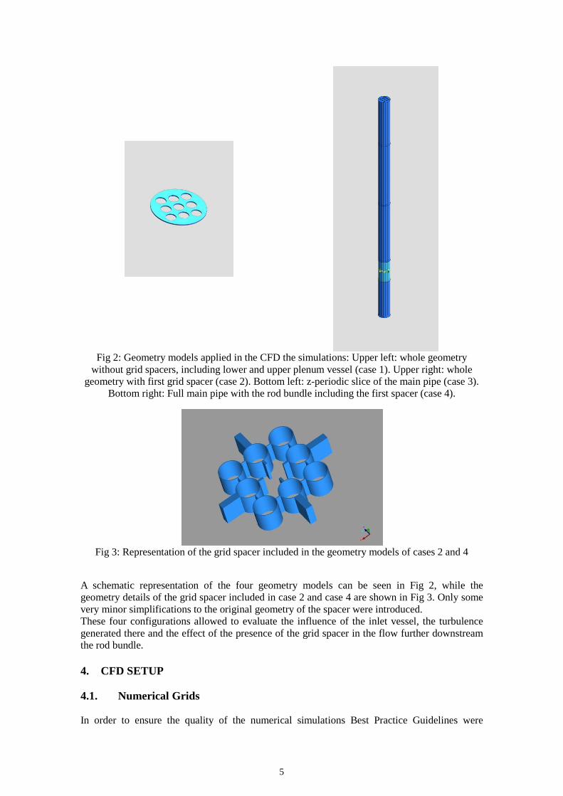
Fig 2: Geometry models applied in the CFD the simulations: Upper left: whole geometry

without grid spacers, including lower and upper plenum vessel (case 1). Upper right: whole geometry with first grid spacer (case 2). Bottom left: z-periodic slice of the main pipe (case 3).

Bottom right: Full main pipe with the rod bundle including the first spacer (case 4).

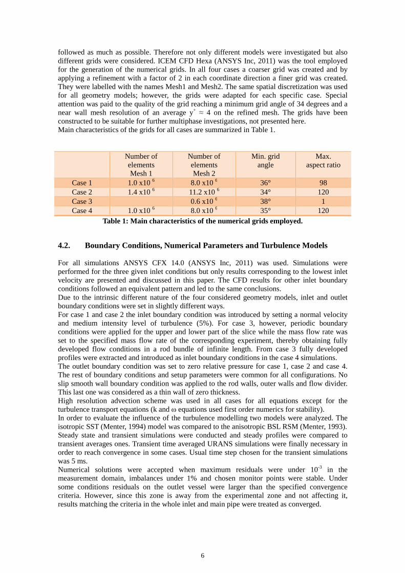
Fig 3: Representation of the grid spacer included in the geometry models of cases 2 and 4

A schematic representation of the four geometry models can be seen in Fig 2, while the geometry details of the grid spacer included in case 2 and case 4 are shown in Fig 3. Only some very minor simplifications to the original geometry of the spacer were introduced. These four configurations allowed to evaluate the influence of the inlet vessel, the turbulence generated there and the effect of the presence of the grid spacer in the flow further downstream the rod bundle.

4. CFD SETUP 4.1. Numerical Grids In order to ensure the quality of the numerical simulations Best Practice Guidelines were

6

followed as much as possible. Therefore not only different models were investigated but also different grids were considered. ICEM CFD Hexa (ANSYS Inc, 2011) was the tool employed for the generation of the numerical grids. In all four cases a coarser grid was created and by applying a refinement with a factor of 2 in each coordinate direction a finer grid was created. They were labelled with the names Mesh1 and Mesh2. The same spatial discretization was used for all geometry models; however, the grids were adapted for each specific case. Special attention was paid to the quality of the grid reaching a minimum grid angle of 34 degrees and a near wall mesh resolution of an average y+ ≈ 4 on the refined mesh. The grids have been constructed to be suitable for further multiphase investigations, not presented here. Main characteristics of the grids for all cases are summarized in Table 1. Number of

elements Mesh 1

Number of elements Mesh 2

Min. grid angle

Max. aspect ratio

Case 1 1.0 x10 6 8.0 x10 6 36° 98 Case 2 1.4 x10 6 11.2 x10 6 34° 120 Case 3 0.6 x10 6 38° 1 Case 4 1.0 x10 6 8.0 x10 6 35° 120

Table 1: Main characteristics of the numerical grids employed.

4.2. Boundary Conditions, Numerical Parameters and Turbulence Models For all simulations ANSYS CFX 14.0 (ANSYS Inc, 2011) was used. Simulations were performed for the three given inlet conditions but only results corresponding to the lowest inlet velocity are presented and discussed in this paper. The CFD results for other inlet boundary conditions followed an equivalent pattern and led to the same conclusions. Due to the intrinsic different nature of the four considered geometry models, inlet and outlet boundary conditions were set in slightly different ways. For case 1 and case 2 the inlet boundary condition was introduced by setting a normal velocity and medium intensity level of turbulence (5%). For case 3, however, periodic boundary conditions were applied for the upper and lower part of the slice while the mass flow rate was set to the specified mass flow rate of the corresponding experiment, thereby obtaining fully developed flow conditions in a rod bundle of infinite length. From case 3 fully developed profiles were extracted and introduced as inlet boundary conditions in the case 4 simulations. The outlet boundary condition was set to zero relative pressure for case 1, case 2 and case 4. The rest of boundary conditions and setup parameters were common for all configurations. No slip smooth wall boundary condition was applied to the rod walls, outer walls and flow divider. This last one was considered as a thin wall of zero thickness. High resolution advection scheme was used in all cases for all equations except for the turbulence transport equations (k and ω equations used first order numerics for stability). In order to evaluate the influence of the turbulence modelling two models were analyzed. The isotropic SST (Menter, 1994) model was compared to the anisotropic BSL RSM (Menter, 1993). Steady state and transient simulations were conducted and steady profiles were compared to transient averages ones. Transient time averaged URANS simulations were finally necessary in order to reach convergence in some cases. Usual time step chosen for the transient simulations was 5 ms. Numerical solutions were accepted when maximum residuals were under 10-3 in the measurement domain, imbalances under 1% and chosen monitor points were stable. Under some conditions residuals on the outlet vessel were larger than the specified convergence criteria. However, since this zone is away from the experimental zone and not affecting it, results matching the criteria in the whole inlet and main pipe were treated as converged.

7

5. RESULTS AND DISCUSSION Only results corresponding to the lowest inlet velocity are included here. Different plots are presented to analyze the numerical results: velocity contour plots, velocity profiles at different elevations, secondary flows and streamlines. These pictures allow us to perform a qualitative and a quantitative analysis of the CFD simulations. 5.1. Experiments Two of the measurement planes were used for the comparison. They are called Plane 2 and Plane 4 and cross the sub-channels of the rod bundle at the centre, providing more information for comparison. The exact positions are indicated in Fig 1. Different elevations along these planes are chosen for the quantitative analysis of the numerical results. They are located at 258 mm and 508 mm respectively above the top of the inlet vessel. A detailed overview of the measured velocity profiles can be seen in Fig 4. Profiles plotted in the pictures correspond to the measurements of the velocity component in vertical direction including the measurement error of ± 6%. It can be observed that for the lowest elevation the profiles are flatter. It is also observable that measurements at these two planes are different even they are located in symmetrical positions, and also that the values at the front of the pipe (negative x axis values) are larger than in the back of the main vertical pipe (front and back with respect to the inlet pipe to the lower plenum). All these phenomena can be addressed to the turbulent inlet configuration. Picture on the bottom left of Fig 4 has no physical meaning. The measurements in that location were corrupted.

Fig 4: Measurement values of the axial velocity minus the measurement error (6%). Left: Plane 2. Right: Plane 4. Elevations at z=198 mm, 258mm,

408mm, 508mm (measured from the bottom of the main pipe)

● Experiment ± 6%

● Experiment ± 6%

● Experiment ± 6%

● Experiment ± 6%

8

: Measurement values of the axial velocity component. Profiles represent measurements plus and minus the measurement error (6%). Left: Plane 2. Right: Plane 4. Elevations at z=198 mm, 258mm,

408mm, 508mm (measured from the bottom of the main pipe)

● Experiment ± 6%

● Experiment ± 6%

● Experiment ± 6%

● Experiment ± 6%

component. Profiles represent measurements plus and minus the measurement error (6%). Left: Plane 2. Right: Plane 4. Elevations at z=198 mm, 258mm,

408mm, 508mm (measured from the bottom of the main pipe)

● Experiment ± 6%

● Experiment ± 6%

● Experiment ± 6%

● Experiment ± 6%

9

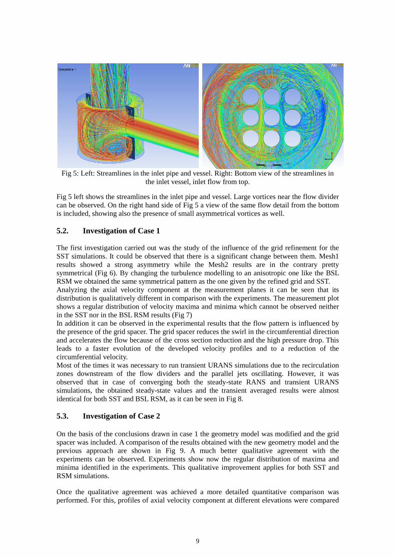
Fig 5: Left: Streamlines in the inlet pipe and vessel. Right: Bottom view of the streamlines in the inlet vessel, inlet flow from top.

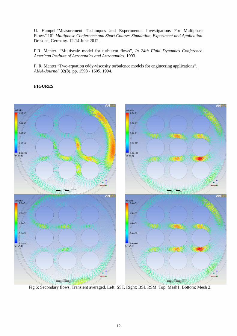
Fig 5 left shows the streamlines in the inlet pipe and vessel. Large vortices near the flow divider can be observed. On the right hand side of Fig 5 a view of the same flow detail from the bottom is included, showing also the presence of small asymmetrical vortices as well. 5.2. Investigation of Case 1 The first investigation carried out was the study of the influence of the grid refinement for the SST simulations. It could be observed that there is a significant change between them. Mesh1 results showed a strong asymmetry while the Mesh2 results are in the contrary pretty symmetrical (Fig 6). By changing the turbulence modelling to an anisotropic one like the BSL RSM we obtained the same symmetrical pattern as the one given by the refined grid and SST. Analyzing the axial velocity component at the measurement planes it can be seen that its distribution is qualitatively different in comparison with the experiments. The measurement plot shows a regular distribution of velocity maxima and minima which cannot be observed neither in the SST nor in the BSL RSM results (Fig 7) In addition it can be observed in the experimental results that the flow pattern is influenced by the presence of the grid spacer. The grid spacer reduces the swirl in the circumferential direction and accelerates the flow because of the cross section reduction and the high pressure drop. This leads to a faster evolution of the developed velocity profiles and to a reduction of the circumferential velocity. Most of the times it was necessary to run transient URANS simulations due to the recirculation zones downstream of the flow dividers and the parallel jets oscillating. However, it was observed that in case of converging both the steady-state RANS and transient URANS simulations, the obtained steady-state values and the transient averaged results were almost identical for both SST and BSL RSM, as it can be seen in Fig 8. 5.3. Investigation of Case 2 On the basis of the conclusions drawn in case 1 the geometry model was modified and the grid spacer was included. A comparison of the results obtained with the new geometry model and the previous approach are shown in Fig 9. A much better qualitative agreement with the experiments can be observed. Experiments show now the regular distribution of maxima and minima identified in the experiments. This qualitative improvement applies for both SST and RSM simulations. Once the qualitative agreement was achieved a more detailed quantitative comparison was performed. For this, profiles of axial velocity component at different elevations were compared

10

to the experimental results. From all the elevations two were chosen for the further assessment: H2=258 mm and H3=508 mm above the inlet vessel. They correspond to a location close after the grid spacer and an elevation close to the uppermost measured position. It must be noted that for the quantitative comparison the CFD results have been scaled. It was noticed that all numerical velocity profiles showed consistently larger velocity amplitudes at all locations than the experiments which may indicate an uncertainty in the provided mass flow rate conditions or difficulties in keeping the inflow mass flow rate constant during the measurements. For a fairer comparison CFD profiles were scaled with a reference factor calculated from velocity maxima at fully developed conditions.

max, ,

,max, ,

0.730.924

0.78subchannel EXPEXP

CFD scaled CFDCFD subchannel CFD

vmv f v with f

m v= ⋅ = ≈ = =

ɺ

ɺ

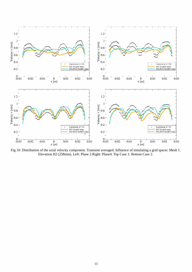
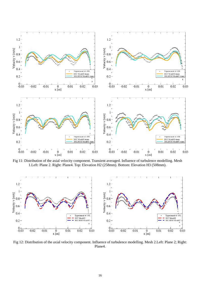
Curves shown on the left hand side of Fig 10 represent case 1 profiles and the ones on the right hand side the case 2 profiles. Case 2 profiles show a considerably better agreement regarding the shape of the profiles, as it was already observed in the qualitative comparison. There is still a shift in location of the velocity maxima and minima, but they are more clearly defined in comparison to the relative flat profiles of case 1. The higher the elevation for comparison is, the better the agreement to the experiments was achieved. The use of the second geometry model improved the quality of the numerical results after the grid spacer. In the area below it was not possible to capture all the mechanisms involved. To overcome this problematic, further analyses were conducted by increasing the turbulence level at the inlet and refining the grid at the inlet pipe and the inlet vessel. However, none of those approached could improve the results comparison. Finally after these investigations these differences had to be addressed to the not very well defined inlet boundary conditions and the pre-history of the flow in the real laboratory test section before the flow enters into the lower plenum vessel. 5.4. Investigation of Case 3 As pointed out in the analysis of case 2, the axial velocity values obtained in the numerical simulations where larger everywhere in the domain than in the measurements. Therefore a new goal was set, which was to be able to accurately predict the flow behaviour at the uppermost position of the measurements, where fully developed conditions are presumed. The influence of the physics at that location should be less influenced by the vortices generated at the inlet vessel where the flow enters the rod bundle configuration. For this purpose the third geometry model was used. It consists of a thin slice of the pipe, where periodic boundary conditions in axial direction and a specified mass flow rate were applied. By conducting this numerical simulation only profile comparison on the uppermost measurement location is appropriate. For this case, the simulations were run with only the finest mesh and allow us to derive a correction (section 5.3) to fit the actually realized mass flow rate in the experiments. As reference point the RSM simulations where considered. Pictures in Fig 12 show that with this configuration we were able to perfectly reproduce the shape of the experiment profiles and the profiles corresponding to the CFD results lie mostly inside the measurement error band. It can be seen that the comparison is slightly better on one Plane 4 than on Plane 2. This is due to the asymmetry of the flow in the experimental test rig caused by the lower plenum vessel and the inlet, as discussed in section 5.1.The CFD results however at the slice can only be symmetrical. This explains the better matching on Plane 4. 5.5. Investigation of Case 4

The approach followed with the third geometry model showed the possibility to accurately predict the behaviour of the flow under fully developed flow conditions, but the intention was to

11

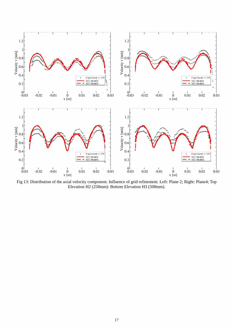
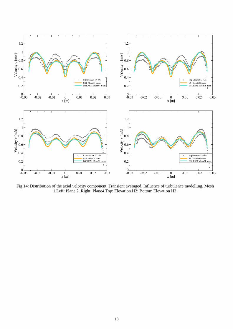
be able to predict the flow in development in the rod bundle at least in the domain downstream of the grid spacer. Due to the described difficulties with the inlet vessel, a fourth geometry model containing only the main vertical pipe, the rod bundle and the grid spacer was considered. For the inlet boundary conditions in case 4 we used the fully developed velocity and turbulence property profiles as they were obtained from the investigations of case 3. The velocity profiles at both planes 2 and 4 and elevations (Fig 13) show that SST results are grid independent. An analysis of the turbulence modelling (Fig 14 and Fig 15) shows that for these conditions, geometry and grid, SST and BSL RSM provide qualitatively similar results, reproducing the behaviour of the flow observed in the experiments. However BSL RSM shows smaller amplitude in the velocity profiles, thereby showing a slightly better agreement with the measurements. This observation can be explained by the fact, that the anisotropic BSL RSM predicts secondary flows of higher amplitude in the rod bundle cross section, which leads to an increased cross-sectional mixing and thereby to reduced minima and maxima in the axial velocity distributions. 6. SUMMARY & CONCLUSIONS Single-phase CFD simulations were conducted in a 3x3 rod-bundle geometry. Different geometry configurations were investigated allowing an analysis of the influence of geometry components like the inlet vessel and the grid spacer. These components play a main role in the evolution of the flow due to the turbulence and vortices generated in the lower inlet plenum vessel and at the grid spacer, which finally influences the symmetry of the flow along the main vertical pipe and through the rod bundle. The spacer grid, on the contrary, reduces the swirl in the circumferential direction and accelerates the flow, leading to a faster evolution of the developed velocity profiles and to a reduction of the circumferential velocity. Best practice guidelines were followed as much as applicable. Therefore grid independency analyses and turbulence modelling variations were performed. The evolution of the four different considered geometry models led to an evolution of the numerical solution in comparison with the measurements: from a qualitative disagreement (case 1) to a qualitative and quantitative agreement (case 4) in the domain above the grid spacer. Flow mechanisms were not completely captured in the inlet vessel and would require further investigations, as well as information about the real inflow conditions in the laboratory test rig. 7. ACKNOWLEDGEMENTS

This research has been supported by the German Ministry of Education and Research (BMBF, Grant No. 02NUK010G) in the framework of the R&D funding concept of BMBF "Basic Research Energy 2020+", the German CFD Network on Nuclear Reactor Safety Research and the Alliance for Competence in Nuclear Technology, Germany.

REFERENCES ANSYS Inc. ANSYS CFX-Solver Theory Guide. Release 14.0. Southpointe. November 2011. ANSYS Inc. ICEM CFD-Users Manual. Release 14.0. Southpointe. November 2011. M. Casey, M. and T. Wintergerst,. Quality and trust in industrial CFD –best practice guidelines. s.l. : ERCOFTAC Special Interest Group on “Quality and Trust in Industrial CFD”, Sulzer Innotec, Fluid Dynamics Laboratory, 2000. E. Dominguez-Ontiveros et al. “Experimental Study of a Simplified 3 x 3 Rod Bundle using DPIV”. CFD4NRS-4. Dajeon, Korea. 10-12 September 2012.

12

U. Hampel.”Measurement Techinques and Experimental Investigations For Multiphase Flows”.10th Multiphase Conference and Short Course: Simulation, Experiment and Application. Dresden, Germany. 12-14 June 2012. F.R. Menter. “Multiscale model for turbulent flows”, In 24th Fluid Dynamics Conference. American Institute of Aeronautics and Astronautics, 1993. F. R. Menter.“Two-equation eddy-viscosity turbulence models for engineering applications”, AIAA-Journal, 32(8), pp. 1598 - 1605, 1994. FIGURES

Fig 6: Secondary flows. Transient averaged. Left: SST. Right: BSL RSM. Top: Mesh1. Bottom: Mesh 2.

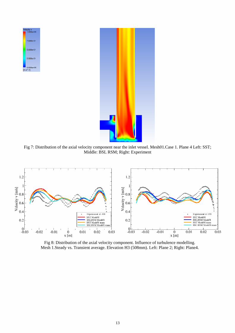
Fig 7: Distribution of the axial velocity component near the inlet vessel. Mesh01.Case 1. Plane 4 Left: SST; Middle: BSL RSM; Right: Experiment

Fig 8: Distribution of the axial Mesh 1.Steady vs. Transient average. Elevation H3 (508mm).

13

velocity component near the inlet vessel. Mesh01.Case 1. Plane 4 Left: SST; Middle: BSL RSM; Right: Experiment

the axial velocity component. Influence of turbulence modelling. Transient average. Elevation H3 (508mm). Left: Plane 2; Right: Plane4.

velocity component near the inlet vessel. Mesh01.Case 1. Plane 4 Left: SST;

. Influence of turbulence modelling. Left: Plane 2; Right: Plane4.

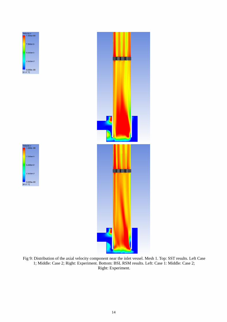
Fig 9: Distribution of the axial velocity component1; Middle: Case 2; Right: Experiment. Bottom: BSL RSM results. Left: Case 1: Middle: Case 2;

14

velocity component near the inlet vessel. Mesh 1. Top: SST results. Left Case 1; Middle: Case 2; Right: Experiment. Bottom: BSL RSM results. Left: Case 1: Middle: Case 2;

Right: Experiment.

near the inlet vessel. Mesh 1. Top: SST results. Left Case

1; Middle: Case 2; Right: Experiment. Bottom: BSL RSM results. Left: Case 1: Middle: Case 2;

15

Fig 10: Distribution of the axial velocity component. Transient averaged. Influence of simulating a grid spacer. Mesh 1. Elevation H2 (258mm). Left: Plane 2.Right: Plane4. Top Case 1: Bottom Case 2.

16

Fig 11: Distribution of the axial velocity component. Transient averaged. Influence of turbulence modelling. Mesh 1.Left: Plane 2. Right: Plane4. Top: Elevation H2 (258mm). Bottom: Elevation H3 (508mm).

Fig 12: Distribution of the axial velocity component. Influence of turbulence modelling. Mesh 2.Left: Plane 2; Right: Plane4.

17

Fig 13: Distribution of the axial velocity component. Influence of grid refinement. Left: Plane 2; Right: Plane4; Top Elevation H2 (258mm): Bottom Elevation H3 (508mm).

18

Fig 14: Distribution of the axial velocity component. Transient averaged. Influence of turbulence modelling. Mesh 1.Left: Plane 2. Right: Plane4.Top: Elevation H2: Bottom Elevation H3.

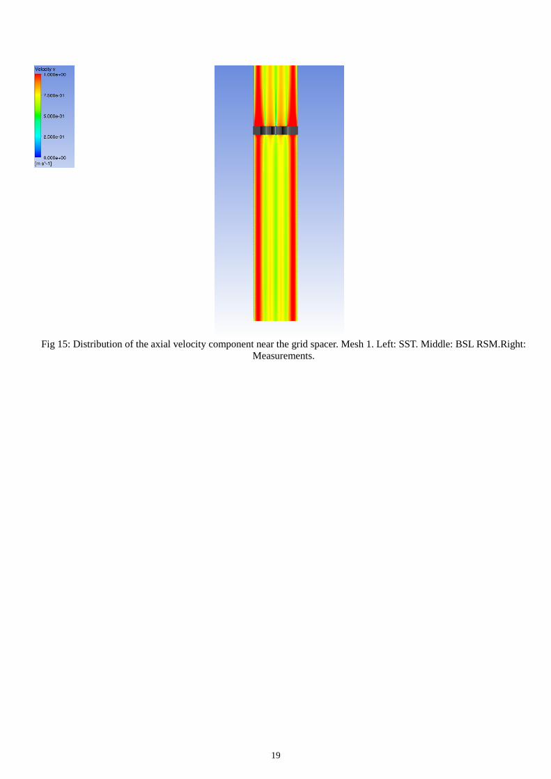
Fig 15: Distribution of the axial velocity component

19

velocity component near the grid spacer. Mesh 1. Left: SST. Middle: BSL RSM.Right: Measurements.

near the grid spacer. Mesh 1. Left: SST. Middle: BSL RSM.Right: