vL.. .~~3

DEPARTMENT OF COMPUTER SCIENCE

UNIVERSITY OF ILLINOIS AT URBANA-CI-AMPAI( A1

T HE N EW A D D ITIO N

3REPORT INO. UIUCDCS-R-90-1626 UILU-EING-90-1 765

5 TOWARDS INTrELLIGENT FINITE ELEMENT ANALYSIS

by DUIC'

Alejandro G. B~lanco C2*u

September 1990 S O T 2 oDISTiUIBUTION STATEMENT A

Appovsd for public reloeas*

SECURITY CLASSIFICATION OF THIS PAGE

REPORT DOCUMENTATION PAGE OMB No.e704d018

1. REPORT SECURITY CLASSIFICATION lb. RESTRICTIVE MARKINGSUnclassified None

2a. SECURITY -CLASSIFICATION AUTHORITY 3. DISTRIBUTION /AVAILABILITY OF REPORT

2b. DECLASSIFICATION /DOWNGRADING SCHEDULE Approved for public release;Distribution unlimited

4. PERFORMING ORGANIZATION REPORT NUMBER(S) 5. MONITORING ORGANIZATION REPORT NUMBER(S)

UIUCDCS-R-90-16266a. NAME OF PERFORMING ORGANIZATION 6b. OFFICE SYMBOL 7a. NAME OF MONITORING ORGANIZATION

Dept. of Computer Science 1 (If applicable)University of Illinois Office of Naval Research

6c. ADDRESS (Cih :e, and ZIP Code) 7b. ADDRESS (City, State, and ZIP Code)1304 W. Springfield 800 N. Quiiicy StreetUrbana, IL 61801 Arlington, VA 22217-5000

8a. NAME OF FUNDING/SPONSORING 8b. OFFICE SYMBOL 9. PROCUREMENT INSTRUMENT IDENTIFICATION NUMBERORGANIZATION I (If applicable) N00014-86-K-0309

8" ADDRESS (City, State, and ZIP Code) 10. SOURCE OF FUNDING NUMBERS

ELEMENT NO NO. NO ACCESSION NO.

1 I. TITLE (Include Securty Classification) i

Towards Intelligent Finite Element Analysis

12. PERSONAL AUTHOR(S)Alejandro G. Blanco

13a. TYPE OF REPORT 13b. TIME COVERED 14. DATE OF REPORT (Year'Month'Day)S115" PAGE COUNTTechnical FROM TO September 1990 I 56I.SUPPLEMENTARY NOTATION

17 COSATICODES -1iB. SUBJECT TERMS (Continue on -reverse if necessary and identify by block number)FIELD GROUP SUB-GROUP/- Finite Element Methods,\achine Learnin &05 10 Explanation-Based Learning, 'Inteiligent Numerical Methods.

191ABSTRACT (Continue on reverse if nece ary and identify by block number) ' r )-)The aim of this research,-s the usa of various artificial intelligence (AI) techniques

to improve the performance of pograms performing finite element analysis, a method thatnumerically solves differential equa t'ons that govern a physical situation. Typically, |a finite element program requires extensie:analysis and frequent interruption by ascientist, which reduces how much the scientisLan learn about the phenomenon being

studied by consuming the scientist's resources andt! in the drudgery of mathematicallyconditioning the input to the finite element program. T 'is work usually has no relationto the matter being studied. This thesis investigates whether AI can be used to reducethe time spent doing this type of work.

' 20. DISTRIBUTION/AVAILABILITY OF ABSTRACT 21. ABSTRACT SECURITY CLASSIFICATION9I:UNCLASSIFIED/UNLIMITED [ SAME AS RPT. C[ DTIC USERS unclassified

! 22a. NAME OF RESPONSIBLE INDIVIDUAL 22b. TELEPHONE (Include Area Code) 22c. OFFICE SYMBOLAlan Meyrowitz 1(202) 696-1.,302 1:ONR

DD Form 1473, JUN 86 Previous editions are obsolete. SECURITY CLASSIFICATION OF THIS PAGEI

iI

3 TOWARDS INTELLIGENT FINITE ELEMENT ANALYSIS

Accession rITIS GRA&I

BY DTI TAB "unannoun oed3 ALEJANDRO G. BLANCO Justflat____a____

B.S., University of Miami, 1989 Dis, b ... ..&_ DIStribution/

Awatlability Codsa

Mat special.

I THESIS

Sutmitted in partial fuilfillment of the requirementsfor the degree of Master of Science in Electrical Engineering

in the Graduate College of theUniversity of Illinois at Urbana-Champaign, 1990

UIi Urbana, Illinois

III

II DEDICATION

IIIaII,I

A Mami y Papi.I ~Que Dios los bendiga!

IIIII£II

iii

I

!ACKNOWLEDGEMENTS

The author wishes to acknowledge the enormous amount of input and help received from

his advisor, Professor Gerald DeJong. Others who have provided insightful comments include

Michael Barbehenn, Scott Bennett, Steve Chien, Melinda Gervasio, Joa Gratch, and Dan

Oblinger. The Cure is credited for inspiration or lack thereof.

The research reported in this paper was supported by the Office of Naval Research under

grant number N0001486-K-0309. The author was supported by an AT&T Fellowship. 3ia!IIIII

iv £a-

TABLE OF CONTENTS

Page

1. IN TRO D UCTIO N ................................................ I1.1 Finite Elem ent Analysis ............................................ 2

1.1.1 Definition ..... ........................................ 21.1.2 An example problem class ...................................... 4

1.2 Explanation-Based Learning (EBL) ................................... 61.3 Qualitative Reasoning .............................................. 10

2. METHODOLOGIES ............................................. 142.1 Object-Oriented Programming ....................................... 142.2 The Finite Element Object-Oriented Solver (FEOS) ...................... 142.3 Im proving Convergence ............................................ 172.4 M eshing Issues ................................................... 18

3. DERIVING APPLICABLE EQUATIONS ........................ 20

4. QUALITATIVE STATES ......................................... 23

5. PRE M ESH ING ................................................... 28

6. CONCLUSIONS AND FUTURE WORK ......................... 31

APPENDIX A. FEOS CODE .................................... 35

APPENDIX B. EQUATION DERIVATION DOMAIN THEORY 43

APPENDIX C. QUALITATIVE STATE DOMAIN THEORY .... 48

R E FER EN C ES ................................................... 50

I

B

1 1. INTRODUCTION

The aim of this research is the use of various artificial intelligence (Al) techniques to im-

prove the performance of programs performing finite element analysis, a method that numerically

solves differential equations that govern a physical situation. Typically, a finite element program

requires extensive analysis and frequent interruption by a scientist, which reduces how much the

scientist can learn about the phenomenon being studied by consuming the scientist's resources and

time in the drudgery of mathematically conditioning the input to the finite element program. This

work usually has no relation to the matter being studied. This thesis investigates whether AI can

be used to reduce the time spent doing this type of work.

When using finite element analysis, a scientist generally follows three steps. In the first step,

the scientist will choose a numerical experiment to run. The second step involves running the experi-

ment by inputting specifications to a finite element program. The third step involves analyzing the

results of this program and deciding if any additional experiments should be run. When analyzing

the finite element results, the scientist must be sure that the results are plausible to preclude round-

off errors and ill-conditioning. This three-step process continues until a sufficient understanding

of the problem area has been attained.

The approach of this thesis is to concentrate on the second step. Modem finite element analy-

sis involves the calculation of many numhers. For this reason, a good deal of effort is appropriately

invested in making finite element programs run as efficiently as possible. One goal of this thesis

is to explore the use of Al to allow finite element programs to run more efficiently. A scientist must

construct numerical experiments and adopt corresponding techniques to ensure the viability of theIII

results. An intuition behind this thesis is that common sense in the form of qualitative reasoning

[Forbus84] can capture the knowledge a scientist usesin this process. Therefore, the main goal of

this thesis is to design a domain-independent finite element program that uses a domain theory about

the phenomenon being studied to intelligently solve the problems presented to it.

Solving finite element analysis problems is inherently repetitive, both within and across

runs. Therefore, a properly designed system might be able to learn from experience to increase its

efficiency. However, identifying what to learn, how to learn it, and how to use it are difficult tasks.

Explanation-based learning (EBL) [DeJong86] is a knowledge-intensive form of machine learning.

Performing EBL with the domain theory described above is a candidate for learning from experience

to increase efficiency.

The rest of this introduction consists of three sections supplying background in finite element

analysis, explanation-based learning, and qualitative reasoning. Chapter 2 of this thesis delineates

the methodologies taken in conducting this thesis, including the description of a novel finite element

object-oriented solver named FEOS. Chapters 3, 4, and 5 describe various approaches to reasoning Iand learning to improve the solver of Chapter 2. Chapter 6 then describes future work and some 3conclusions.

1.1 Finite Element Analysis

1.1.1 Definition i

Finite element analysis is the use of numerical techniques to approximately solve a set of Idifferential equations governing a physical phenomenon. Examples of physical phenomena for

which finite element analysis is used include material deformation, heat transfer, electromagnetic

2

field dissipation, and fluid flow. The area where the phenomenon occurs is divided into elements

of finite size, whose borders are defined by nodes. The number of nodes that define an element is

known as the degree of'freedom of that element. The set of all elements in a problem is referred to

as the mesh. A mesh may be comprised of elements of different shapes, sizes, and degrees of free-

I dom. Figure 1 summarizes these definitions.

Ilit node........-

* element mesh

*-- 1 1 1 1. 1 1

Figure 1. A Sample Mesh

The goal of finite element analysis is to find the values of the unknown parameters at the

£ nodes and, therefore, have the whole solution by interpolation across each element. Locd linear

algebraic equations defining the relationship betwseen the parameters at the different nodes Awithin

an element are derived from the differential equations that govern the physical phenomenon b% as-

Ri suming small parameter variations across the element. The small variation assumption requires

small elements and this necessitates the large number of elements that are typical of finite element

i problems. These equations can be viewed as local constraints on the parameters. Since nodes are

shared by neighboring elements, and the values for the parameters at a node must be the same for

all elements that share the node, there are compatibility constraints on the parameters to ensure

33£

consistent solutions. Additional constraints are supplied by boundary conditions, which are param- 1eter values at particular nodes specified as part of the problem. The solution at each node is found n

by simultaneously solving the set of local equations after application of the bounda'y conditions and

ensuring that the compatibility constraints are satisfied. This is known as solving the mesh. Tradi- !

tional finite element programs solve a mesh by assembling the local equations into astiffness matrix, 5K, replacing any values known by boundary conditions, and then solving the equations using highly

optimized matrix manipulation techniques. An example showing the stiffness matrix used in tradi- U1

tional methods is included in the following section. Finite element programs spend most of their irun time in solving these equations.

I1.1.2 An example problem class

To facilitate analysis, a simple one-dimensional problem class is-used as-an example. The 5problem is a beam under loads. Figure 2 shows a three-element single force-example and the node 3

//.--7node 2"*/ 0 2 32// 3

"C element

Figure 2. Three-Element Example and Numbering Conventions

and element numbering conventions. The unknowns are 3(1) the stress, or the internal force or tension, for each element, 3

41

1

(2) the strain, or the change in length due to compression or expansion, for each

I element,

(3) the external force at each node,

(4) and displacement at each node.

Locally, the stress,f, positive for expansion by convention, and the strain, which is the difference

I between the right displacement, dR, and left displacement, dL, both measured positive to the right,

are related by

f = k(dR-djL), (1)

Iwherej k = AEIL, (2)

A = the cross-sectional area,

I, E = the modulus of elasticity, and

L = the original length.

Figure 3 summarizes the va-iable naming conventions. The compatibility constraints are that neigh-

boring elements, i and i+J, must agree on the nodal displacement they share, and their stresses must

equal the external forces at the node, i+1, in this case. These can be written as

' dR[i] = dL[i+1], (3)

and F[i+J] =f[i]-f[i+1], (4)

I' respectively. In traditional finite element analysis, the notation would be

xi = dR[i-l] = dL[i], (5)

and Fj = F[i+l]. (6)

I1!I

II!

left displacement (dL) right- displacement (dR)1

/

stress or internal force (f)

Figure 3. Variable Naming Conventions 5

This results in

F, k, -k 0 -.----------- 0 X1, -kj kj+k2 -k2.. -. ,

0-.-k2 k2+k3.

= , : =Kx= " .43 0. % -kn 1 k .

kn +k -kaF, 0------------ 0 -

as the set of equations to be solved for an n-element problem, where K is the stiffness matrix. The

bounda'y conditions would then be inserted and the set of equations would be solved for the un-

known Fi's and .i's.

1.2 Explanation-Based Learning (EBL)

Explanation-based learning [DeJong86] is learning with background knowledge. When an

intelligent being encounters an example of something it wishes to learn, it references its-memory

in-an attempt to understand the example. If the being is able to build an explanation for the-example

in terms of its background knowledge of the world, then the being can learn from the example by

ii

I

5 remembering the conditions under which the explanation holds and the resulting information. This

"1 can then be summarized by a rule that has preconditions, or antecedents, and consequents. In this

way, the explanation does not have to be regenerated when the learned information is desired. Addi-

SI tionally, the preconditions and consequent can be generalized so that the new rule can apply to more

3I than just the example seen.

The task is more rigorously stated in Table 1. The explanation generation task is one of sim-

I Table 1. The Explanation-Based Learning Task [Mitchell86]

Given:, • Target Concept

u • TRaining Example

0 Domain Theory: a set of rules and facts used to explain the training example

* Operationality Criterion: a specification of the form of the learned rule

Determine:

£ .A generalization of the training example that is a target concept description

and satisfies the operationality criterion

j ply proving the example is correct using memory contents expre.sed as facts and rules. Seeral

I methods for learning and generalization are available [Mitchell86], (Mooney86], but the EGGS

method [Mooney86] is preferred because of its efficiency and simplicity. The basic idea is to search

3 until an explanation has been found. The top of the explanation forms the consequent and the bottom

II!

forms the antecedents. Generalization is accomplished by removing any variable bindings to the 3specific example, thus retaining only those necessu-y for the explanation to remain valid. a

A classic example, taken from Mitchell et al. [Mitchell86], is that of recognizing a cup. Us-

ing the domain theory in Table 2,1 one can explain the training example in Table 3 with the explana- 1

Table 2. A Partial Domain TheoryI

liftable(X) A stable(X) A open-vessel(X) =* cup(X)

is(X,light) A part-of(X,Y) A is-a(Yhandle) * liftable(X)part-of(X,Y) A is-a(Ybottom) A is(Yflat) stable(X)

part-of(X,Y) A is-a(Yconcavity) A is(Yupward) open-vessel(X)

Table 3. A Cup Training Example jcup(objectl) is(objectl,light) part-of(objectl ,handle 1)

part-of(objectl,concavity 1) part-of(objectl,bottom 1) is-a(handle 1,handle)

is-a(bottom 1,bottom) is-a(concavi ty 1,concavity) is(bottom 1,flat)

is(concavity I ,upward)

Ition in Figure 4. The learned rule fr'om this example is i

is(X,light) A part-of(X,Y) A is-a(Yhandle) A put-of(X,Y) A is-a(Ybottom)

A is(Yflat) A part-of(X,Y) A is-a(Yconcavity) A is(Yupward) * cup(X).

A is the symbol for conjunction, or logical AND, and = is the symbol for logical implication

I

i cup(objectl)

.I ... .....

liftable(objectl) stable(objectl) open-vessel(objectl)I5 is(objectl .light) part-of(object 1 ,bottom 1) part-of(object 1,concavity 1)

part-of(objectl ,handle 1) is-a(bottom 1 ,bottom) is-a(concavity 1 ,concavity)5 is-a(handle 1,handle) is(bottom 1,flat) is(concavity 1,upward)

Figure 4. Explanation For the Cup Example of Table 3

3The concept of an operationality criterion is one that has been difficult to define. However,

as can be seen from the example, it is necessitated by the fact that a nonoperational definition o" the

target concept is already-known. This leads to the conclusion that what is to be learned is essentially

3already known. Therefore, an operationality criterion defines the utility of EBL in that the goal is

to operationalize a nonoperational concept description. Although this may seem of-little value, the

fact is that with a large amount of information, the concept may never-be discovered without the

I example. Explanation of the example is a highly constrained search through this information be-

j cause many hypothetical considerations are not encountered.

In order to use EBL to improve finite elements, the task must be rigorously stated as sug-

gested by Mitchell et al. [Mitchell86]. The inputs should be defined as

I- - Target Concept: good decisions at choice points in a finite element program,

3 . Training Example: examples from previously solved problems,

I

I* Domain Theory: a domain theory that can explain decisions must be used. Qualitative rea-

soning, described in the next section, is a candidate for this domain theoy. a* Operationality Criterion: preconditions that can be recognized at the decision points. i

1.3 Qualitative Reasoning

Qualitative reasoning [Forbus84] is reasoning about situations nonnumerically. Through

reasoning about confluences between parameters, many interesting conclusions, such as possible 3future states or causes for state changes, can be determined. Some modified examples, taken from aForbus [Forbus84], of questions that can be answered with qualitative reasoning are shown in Figure

5. As shown in these exunples, qualitative reasoning can be used to explain as well as predict physi- 3cal situations.

Confluences between parameters are represented as qualitative proportionalities, referred to

as "'q-props," or inverse qualitative proportionalities. Whenever there is a nonconflicting set of q-

props and inverse q-props to a parameter, X, it is known to be increasing, decreasing or constant. 3A nonconflicting set occurs when all the nonconstant parameters that are q-prop toXare all increas-

ing or all decreasing, and similarly for nonconstant parameters that are inverse q-prop to X, and that

if the nonconstant q-prop parameters are increasing, then the nonconstant inverse q-prop parame- 3ters are decreasing or vice versa. Table 4 shows a domain theory that encodes the nonconflicting

set of q-props (Q+) and inverse q-props (Q-) concept and supports the conclusions made in the first

example of Figure 5. An explanation structure for question Q2 of Figure 5 is shown in Figure 6.

Many of the available qualitative reasoning techniques have not been used in this research.

The usefulness of qualitative reasoning for finite element analysis is in its ability to codify the type

10

Q 1: What mnight happen? Q3: What hap~pens if tihe block is released?

A: The water inside miight boil, and if the A: Assumning the spring doesn't collapse, the block will oscillate

pot is scaled it mnight blow tip. back and forth, and if there is friction, it will eventually stop.Q2: Why miight it blow up? Q4: Why would friction cause it to stop?

, A: A scaled pot would fix the volume A: Friction produces a force in a direction opposite to that ofand mass, and pressure would in- motion. A force will cause ail acceleration in its direction,crease solely with temperature. lIf the and thuts the frictional force will cause a deceleration, Sincepressure goes above a certain value, the amiount the block moves is directly lproportionai to itsthe pot will blow tlp. velocity at the beginning of each oscillation and the deceler-

ation is reducing this velocity, the block will even~tually stop.

' Figure 5. Some Questions Qualitative Reasoning Can Answer

I

of knowledge used by a scientist when designing finite element programs. This is done through-thedefinition of qualitative domain theories that can be used with EBL to explain and len about deci-

3 Asions made in solving finite element problems.

po ssae tmgtbovu.bc n otadi hr sfitoi ileetal tpQ2 h ih tbo p 4 h wudfito as tt tpA:Asae Itwudfxtevln :Fito rdcsafrei ieto poiet hto

I

Table 4. A Partial Domain Theory and Base Facts for Question Q2

Domain Theory:Q +(temperature,pressure) Q+(heat,temperature)Q-(volume,pressure) Q+(mass,pressure)value-for(X,Y,Z) A

(V W, Q+(WY) value-for(VWZ) A-(increasing(V) v constant(V))) A3

(V W, Q-(WY) value-for(VWZ) A (decreasing(V) v constant(V)))* increasing(X)

value-for(X,Y,Z) AI(V W, Q+(WY) value-for(VWZ) A -(decreasing (V) v constant(V))) A

(V W, Q+(WY) value-for(VWZ) A (increasing(V) v constant(V)))=* decreasing(X)X < Y A increasing(X) =* eventual ly-greater(X,Y)

being-heated(X) A value-for(Yheat,X) => increasing(Y)sealed(X) A containS(X,Y) A value-for(Z,volume,Y) =* constant(Z)sealed(X) A contains(X,Y) A value-for(Z,mass,Y) =* constant(Z)Ivalue-for(X,temperature,Y) A i ncreasing(X) A

noninsulating(X) A contains(X,Y) A value-for(Z,tempeirature,Y) =* increasing(Z)jvalue-foir(X,pressure,Y) A contains(YX) A

bursting-pressure(YP) A even tual ly-greater(X,P) := eventually-blows-up(Y)intact(X) A contains(X,Y) AIvalue-for(Z.pressure,Y) A bursting-pressure(YP) A value(Z,P) =* P < PBa

Base Facts:val ue-for(c-pressuire,pressure,c on tents) contai ns(pot,contents)being-heated(pot) noninSLulating(pot)bursting-pressure(pot,pb) intact(pot)

value (c-press ure, p) sealed(pot)Ivalue-for(c-te mperature, temperature,con tents) value-for(c-vol ume ,volume,contents)value-for(p-temnperature,tempeirature ,pot) value-for-(c-mass,nmzss,conterns)I

123

IN

N2 N3 N4 N5

N6NN8 N4 N2 N5 N9 N12 N2 N1O Nil N15 N13 N14 N18 N16 N17

NIL N20 N4 N21 N2 N22 N4 N14 N22 N4 N17

I AN23 N24

NI: eventually-blows-up(pot) N 13: Q+(mass,pressure)IN2: value-for(c-pre ssure,press ure,con ten ts) N 14: va lue-for(c-mass, mass ,conten ts)N3: eventual ly-greater(c-pressure ,p b) N 15: constant(c-mass)N4: contains(pot,contents) N 16: Q-(volume,piressure)IN5: bursting-presSuire(pot,pb) N 17: value-for(c-volu me,vol uine,con tents)N6: c-pressure < ph N18: constant(c-volume)N7: increasing(c-pressure) N 19: value-for(p-temperatur~e,temper'aturie,pot)IN8: intact(pot) N20: increasing(p-temperature)N9: value(c-pressure,p) N2 1: non insulating (pot)N 10: Q+(temperature,pressure) N22: sealed(pot)N Nil: value-for(c-temper-aturie,temper-aturte, N23: being-heated(pot)

contents) N24: value-for(p-heat,heat,pot)N 12: increasing(c-ternperature)

Figure 6. Explanation for Question Q2 of Figure 5

31

I

2. METHODOLOGIES

This section L. scribes a novel finite element solver and the methodologies used in trying to

improve its performance via application of AI techniques. These techniques have all been tested

for the example problem class described in Section 1.1.2. More complex problem classes might be

better targets for the application of Al techniques because there are more areas where complexity Ican be reduced. Additionally, the techniques found useful in this domain may not be scalable to more acomplex domains. However, the simple problem class allows discussion of many introductory is-

sues and allows implementation of more techniques. The issue of scalability is addressed for each Bof the candidate techniques described.

2.1 Object-Oriented Programming

Object-oriented programming [LaLonde90] involves defining data items as objects which

are instances of object types and any actions to be performed on these data items as operations asso-

ciated with the object type. Once the object types and operations have been defined, a task can be 3delineated in terms of operations to be performed on objects. In top-down programming, once lower

level procedures and functions have been written and debugged, they are called to perform tasks

without regard to how the tasks are performed. Similarly, in object-oriented programming, once

the object types and operations have been written and debugged, they are called without thought of

how they perform the desired tasks.

2.2 The Finite Element Object-Oriented Solver (FEOS)

In order to facilitate the study of various approaches to learning for finite element analysis,

a novel finite element solver, named FEOS, has been designed. FEOS is an object-oriented solver

14

that represents each element as an object and has operations that contain the local constraints. FEOS

has been implemented in the Flavors System of Lucid Common Lisp on an IBM RT,2 and the code

has been included in APPENDIX A. The elements enforce the compatibility constraints by commu-

nicating with neighboring elements. Essentially, an element propagates shared parameter valut.. to

its neighbors whenever it changes any of its parameters, while maintaining its local constraints. In

this way, when no more messages are being sent, all compatibility constraints have been met and

the solution has been converged upon. The main activity of an element upon the receipt of values

from its neighbors is summarized by the following pseudo code:

if values are inconsistent with compatibility constraints

compensate for compatibility constraints

with decision procedure (I)

re-establish local constraints

with decision procedure P

send mess, ge(s) to neighbor(s)

endif

The element may have several alternate ways of accomplishing the compensation and reestablish-

ment steps. For example, suppose element A receives a message that a neighbor, B, has a value, .x,

for the displacement at the bordering node, and that A has a value, .4, for the displacement. If .rA

5x , A can-change its value to xB and compensate by changing its stress to agree with the new strain.

It could, on the other hand, set its value for the displacement to any value between XA andxB and again

2 RT is a trademark of International Business Machines Corporation

15

compensate by changing its stress. It could, as well, for both of the above alternatives, absorb the £change in the displacement only partially with the stress and partially with a change in its other dis-

placement. These choices are all seemingly arbitrary at the element level, but certainly will affect

the speed of convergence. This example shows the necessity of the decision procedures, (D and r.

The decisions 0 and F must make are

(1) whether to meet, undercompensate, or overcompensate for an incompatibili-

ty, i.e. given a parameter, A, with a value x, and the receipt of a message with

a value of y > x for A, should the new value for A be y, x < z < y, or z > y,

and

(2) which parameters to change given an incompatibility.

Experimentation in terms of efficiency and -convergence results in heuristic default definitions for

these decisions that have been built into FEOS. The defaults are that (D specifies setting the contested

parameter, A, to the average of its value and the-value received in the-message, (x+y))/2, and r speci-

fies changing the stress first, if possible, and as little else as possible to compensate. There are no

analytical claims made about convergence of FEOS on a solution, but empirically FEOS converges

on the solution for 98% of all examples run.

A system that is to use AI techniques must be able to reason about

(1) a single element,

(2) all elements, or

(3) a set of elements.

16

I

In traditional finite element techniques, the elemental equations are assembled into a matrix that

1l must then be solved. Therefore, there is no way to insert additional knowledge into an element. The

fact that FEOS is object-oriented and the way it is organized facilitate the application of Al tech-

Im niques to finite element analysis. With FEOS the types of reasoning described above can each be

Iaddressed by

1 (1) reserving an area in the element object type that is to contain element-specif-

ic knowledge to be used by the operations,

1 (2) reserving a global area to be used by the operations, and

1(3) either of the two above methods with a membership function to determine

which elements use which parts of the knowledge if a global area is used.

Additionally, elements can be reasoned about in a natural fashion because the division of the ele-

ments into objects encapsulates all elemental information. Specifically, all parameter values and

convergence steps can be analyzed at the individual elements.

I With FEOS, the task of improving finite element analysis becomes one of improving FEOS.

The remainder of this thesis describes different approaches to inserting intelligence into FEOS in

1an attempt to improve its performance.

1 2.3 Improving Convergence

I Section 2.2 identified several decisions for which FEOS has heuristics. One approach to im-

£ proving FEOS is to improve its convergence behavior by learning justifications for these decisions.

One way to attack this task is to learn additional constraints for the elements. The goal in learning

3 constraints is to add global constraints to the local constraints already known at the elemental level.

£17

II

These constraints can then be used to restiict the possible decisions. For example. consider a con-

straint that requires that an elemental parameter, A, with a value .A, greater than or equal to some

number, xL, and a message with a value xB forA arrives. If.rB < xL, then A cannot be set to.rB. Addi-

tionally, it is known that xB is an incorrect value for A.

A quantity lattice [Simmons86] can take as input the equations and boundary conditions of

a problem and determine many constraints, such as bounds on parameters and inequalities and

equalities that exist between different parameters. However, it is possible to establish an arbitrary

number of constraints between arbitrary parameters and expressions involving parameters. There- 1fore, it is necessary to determine which additional constraints would be useful. Two specific types

of constraints have been identified. Studies of their utility are presented in subsequent sections. The

basic premise is that qualitative knowledge can be used to determine which constraints to learn. 52.4 Meshing Issues 1

Meshing issues come down to the attempt to resolve a tradeoff between minimization of n

mesh density and accuracy, where mesh density is the number of elements per mesh area. The idea

is that less calculation is necessary to solve a mesh with fewer elements, while accuracy goes down Iwith a coarser mesh, because the assumption that parameters have small variations across an element 3used to derive the local constraints is less valid across larger elements. 'I

Resolution of this tradeoff can be approached with intelligent initial meshing. Although

there is no inherent advantage for FEOS in terms of solving a problem once a mesh has been deter- -mined, the determination of which elemental borders should be removed is facilitated by the object-

oriented approach used in FEOS.

183

I

3A second approach to resolving the meshing tradeoff is the use of a dynamic mesh that allows

1 elements to fuse and split during solution of the equations. This aptroach is not implementable with

traditional finite element solution techniques because any change in the mesh during solution would

I require the assembly of new matrices and any work done to that point would be meaningless. FEOS

5 can easily fuse or split elements by simply retaining all intermediate parameter values and interpo-

lating values for any new nodes. Convergence can then continue from this point. Fuse/split deci-

sions can be made and learned about. Although this thesis does not contain any results on dynamic

mesh proposals, it appears that the use of a qualitative domain theory that can explain how fuse/split

decisions can affect gradients is a promising avenue for future research.

1

III

I

I

1 1

3. DERIVING APPLICABLE EQUATIONS

One approach to learning a specialized constraint is to learn a ratio, 0, between two elemental

parameters, X and Y, adding the constraint X = OY. It must be known that X and Y have a linear

relationship, but this type of relation is very common in finite element analysis because of the formu-

lation of the problem into a set of linear equations. For the example problem class, boundary condi-

tions specify either the displacement or the external force at each node an the other is an unknown.

Therefore, for every element, X is the unknown for the '-ft node and Y is the dnknown for the right

node. A domain theory, reproduced in APPENDIX B, has been developed that explains 0 for an

element by explaining why X and Y take on the values that they do. The domain theory is composed

of rules of the following form:

value(Element,Z,z)

pl(Element) ; preconditions

pn (Element)

f1(xj,Element) ; subexpression

fm (Xm, Element)

z = f(x 1 , . . / ,X )

20

I

3Rules of this form say that if conditionspl through p, hold for Element, then the elemental parameter

I z = f(,.... ,), where x.,. .. ,.n are calculated viaj .. . f. Explaining a ratio, therefore, is

3 equivalent to deriving an expression for it, namely, f(xj, .... );). This expression is in terms of sub-

3 expressions, x, ... ,.", that must also be derived in terms of subexpressions, until x1 , .... are

3all elemental parameters. The number of subexpressions and preconditions for z is (n+m), usually

a small constant. However, the number of levels of subexpressions will grow with the number of

I elements and since the solution must be searched for, the search is exponential in the numbei of ele-

3ments. This implies that although the method may work for small examples, it will not scale up to

more realistic examples because an exponential space must be searched.

Since the search is-through a large space, this task would normally be a good candidate for

EBL which can help guide the search through the use of-the example being- explained. However,

3 in this case, the example is the ratio from a solved problem in the form ratio(elementX,x), where .

is a number. The numerical answer cannot be tested against alternatives at a node in the search space

I since the alternatives represent different expressions and their numerical values cannot be deter-

3 mined until the expression is known. The expression is known only after the subtree at the alterna-

tive has been searched. Therefore, the utility of searching an alternative cannot be precomputed and

I thus no search can be saved.

- A system that explores these ideas, and on which many of the results described are based has

been designed and implemented. It consists of an EBL Lisp program that explains examples and

learns from them, and the domain theory in APPENDIX B. The problem of complex rules becomes

23 2

very evident from a direct application of EBL to this domain theory. A three-element program pro-

duces rules with 80 antecedents. However, it may be surmised that many of these antecedents are

superfluous due to subsumption by cther antecedents in the rule. The application of truth-preserving

subsumption-removal transforms to the aforementioned rule results in only 19 antecedents remain-

ing. The form of this rule, however, shows that there are conclusions drawn from the state of each

element and thus the complexity of the rule is in terms of the number of elements.

22

I

14. QUALITATIVE STATES

5 Qualitative reasoning allows one to conclude that an object is in a certain state. Once the

3 state of an object is known, certain equalities and inequalities can be known to constrain the object.

One approach to learning specialized constraints is to detect when an element is in a qualitative state

I and use the implied constraints to restrict choices.

IFor the example problem class, an element can be provably in compression or expansion.

Proving an element is in compression or expansion involves external forces and the-f ict that an ele-

ment is a member of a bar that is eventually fixed on one side. For example, in Figure 2, elements

31 and 2 are provably under compression and element 0 is provably under expansion. An explanation

for element 0 being underexpansion is shown in Figure 7. A domain theory that can be used to deter-

mine the compression/expression states of elements is included in APPENDIX C.

I If an element is known to be in compression or expansion, then the sign of the stress is known.

3 ! Therefore, whenever an incompatibility is encountered by an element, it can restrict compensating

parameter changes to only those which will not cause the sign of-the stress to be the opposite of what

is known to be the final sign. More specifically, whene, er the default (1) and r propose the alteration

3of the stress, the state of the element after the proposed alteration is checked againstthe known final

state,- and alternative compensations are performed if these states conflict. Alternatives are the

changing of parameters other than the stress. Three versions of FEOS exist. They are

• * FEOS, which has the default O and F and no knowledge of the compression/expansion state

I of the elements in a problem,

I1 2

II

expansion elementO)

net-external-force(F,elementO,iight) F > 0 eventually-fixed(element0,1eft)

external-force(node 1,F) external-force(node2,0) external-force(nodie2,O) F = F + 0 + 0

boundary-condition(node3,displacement,O) boundary-condition(element0,1eft,displacement,O)Iboundary-condition(element2,right,displacement,O) 3

Figure 7. Explanation of Element 0 Being under Expansion 5

" FEOS-USECE, which is FEOS with (D1 and F modified as described above and knowledge

of the compression/expansion state of the elements in a problem, and 3* FEOS-REPORT, which is FEOS with the default (D and F, knowledge of the compression/

expansion state of the elements in a problem, and a modification to the main loop so that any

time an element is not in its final state the fact is reported to the screen. 3It is unclear whether having the compression/expansion information helps FEOS converge

faster or not. Figure 8 shows the result of a test of the hypothesis. The bottom axis represents a set

of examples with roughly increasing complexity to the right, and the left axis represents the number Iof messages propagated. The results show no systematic comparative out-performance or under- 3performance between FEOS and FEOS-USECE in the number of propagations needed to converge

on a solutioni.

24 1

11

I

5400-

1m 4800. FEOS

3 4200- FEOS-USECE

3600-

Propagations 3000.

I 240.

1800.

1200.

600-

Examples

Figure 8. Evaluation of Compression/Expansion State Knowledge on General Examples

3The low, and sometimes negative, utility of this information may be due to the fact that the

heuristic built into the solver tends to lead elements into the final state and-thus little is gained. Con-

I versely, it may be that certain problems require that elements be in states other than their final state

5 during convergence, while others require that the elements be in their final state during convergence.

The latter of these types of problems would thus gain by knowing the final states and the former

Iwould lose by knowing this information and converge more slowly. One way to determine which

5 of the two possible explanations given above is the case is to design a set of examples for which solv-

ing by FEOS-REPORT yields a large number of out-of-state reports. If the former of the explana-

tions for the low utility of the state information is the case, then the state information would cause

the convergence for these examples to be improved. One such set of examples is that comprised of

examples of the form shown in Figure 9. For these examples, the elements between the left and right

325

iiI

F>f f

Constant Material Properties gFigure 9. The Form of Examples Usually Out of State

forces will eventually be under compression because the left force is greater than the right force. IHowever, those elements just to the left of the right force will receive messages which cause them -

to be in the expansion state when the problem is being solved without the state information. When

FEOS solves this example set using the state information, there is a degradation in convergence per-

formance, shown in Figure 10. This suggests that the later explanation for the low utility of the state 3information is the case. g

26

II

I

II4 I

24000-210001 FEOS18000- - FEOS-USECE18000- -_ i

Propagations 10

i ~ ~12000Y ..

9000-6000- /

3000. . -

Examples

Figure 10. Evaluation Of Compression/Expansion State Knowledge On ExamplesUsually Out of State

I

I

1 2

I5. PREMESHING I

Many of the approaches discussed in Section 2.4 on meshing issues are as yet unexplored. IHowever, one meshing method which has been investigated involves qualitatively preprocessing

an initial mesh to determine boundaries that are removable by the replacement of bordering elements

with a quantitatively identical element. This method assumes that some nodes are not removable Ibecause the parameter values at these nodes are goals of the analysis. Therefore, the method is given

goals in tcrms of nodes that are not removable. This method examines each boundary to determine

whether or not it is removable given the goals, a specification for the problem, and a boundary re- Imoval domain theory for the problem class. If the bounday is removable, then the elements that Ushare that boundary are replaced with a single element across the boundary. For example, consider

Example 3.1 from Logan [Logan86] shown in Figure 11, and the boundary removal domain theory II

A=l in.2 A=l in.2 A=2 in.2

E=3 × 107 psi E=3 x 107 psi E=15 x 106 psi .

4 3000 Is.[

30 in. )04 30 in. -04 30 in. --- 05

Figure 11. Example 3.1 from Logan [Logan86] of the Example Problem Class

shown in Table 5. The boundary at node 2 can be removed and the problem reduced to a two-element

problem by replacing elements I and 2 with a single element with aggregate length, length-averaged icross-sectional area, and volume-averaged modulus of elasticity.

28

II5 Table 5. A Boundary Removal Domain Theory

greater(Node,0) A number-of-nodes(NumbeOfElements) A

less(Node,NumberOfElements) A no-goals(Node) A no-discontinuities(Node)=* removable-boundary(Node)

goals(Goals) A not-member(Node,Goals) no-goals(Node)I external-forces(Node,0) A boundary-condition(Node,force)* no--discontinuities(Node)

This method is implemented and results in obvious improvement in terms of propagations,

shown in Figure 12, because it reduces the problem to one containing fewer elements. The bottom

1 8000-- Without Premeshing

7000-- - With Premeshing

6000-

3 Propagations 5000-

4000-

S30002000-

3 1000 -

0-

3 Examples

3 Figure 12. Evaluation of Premeshing by Propagations

3 axis is an example set with roughly- increasing complexity to the right. Since time is consumed in

preprocessing the mesh, simply reducing the number of propagations does not constitute a net

29

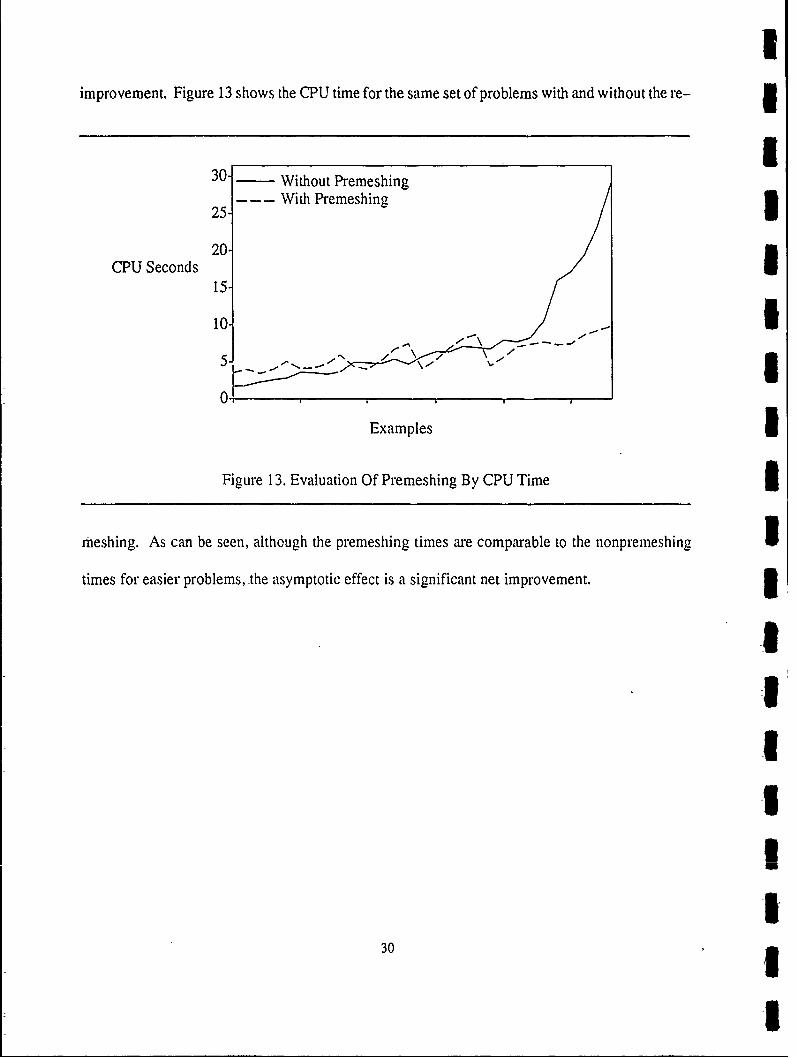
Iimprovement. Figure 13 shows the CPU time for the same set of problems with and without the re-

___ I30. - Without Premeshing25. With Premeshing 3

CPU Seconds 15

15. -"

10 15-0

Examples UFigure 13. Evaluation Of Premeshing By CPU Time 3

meshing. As can be seen, although the premeshing times are comparable to the nonpremeshing Itimes for easier problems, the asymptotic effect is a significant net improvement. 3

3

30 11

I

I 6. CONCLUSIONS AND FUTURE WORK

3 FEOS is a novel finite element solver that appears to be a good vehicle for the application

g of Al to finite element analysis. The use of qualitative domain theories for learning constraints on

elements seems to be a reasonable approach to constraining underconstrained decisions at the ele-

I mental level. Aside from intelligent premeshing, no clear path to improvement of finite element

3analysis program, has been found. However, the space of possibilities has been mapped out and

experimentation into the different possibilities is the true test of the feasibility of the task.IIn a somewha t related work, Abelson et al. (Abelson89] have shown that Al techniques can

3 be used to aid scientists in scientific computing by developing tools that are useful when setting up

and running nimerical experiments. They do not, however, address finite element analysis directly.

Dynamic meshing, a, well as many other meshing options, has not been studied in depth.

I This-area would seem to have , good chance of having justifiable decisions because scientists must

3 explicitly reason about what does and does not make a good mesh. The design of a domain theory

for these decisions and operations in FEOS that can use this theory to fuse and split-elements is an

obvious path for future research.

IThe utility of qualitative states is not well understood. Careful study of the-examples for

3 which the compression/expansion state information is useful and examples for which it is harmful

is necessary. Common aspects in the two sets might be insights into what these states are actually

Icontributing. Additionally, other qualitative states might be identifiable and usable.

UAll parameter changes in an element are directly explainable in terms of the message just

I propagated to it. Therefore, if all parameter changes are explained, a large explanation can be

331

I

constructed that has these individual parameter change explanations as subexplanations. It may be

possible to recognize loops or repetitions comprised of multiple parameter changes that can be re-

duced to a single parameter change. To do this, these loops must be explicable in terms of eventual

convergence, and detectable by an element in a convergence step. If a domain theory that can do 3this can be written, this approach may be extremely useful. One possibility is the use of axioms simi- 5lar to those used by Minton et al. [Minton89] in the planning domain. These axioms might codify

the nonutility of iterations that move away from the eventual correct answer and the utility of moving

toward the eventual solution. 3In the equation derivation approach of Chapter 3 the equations became too complex for effi-

cient development and usage in realistically complex problems. The operationality criterion used

is that all expressions must be in terms of elemental parameters and that all preconditions be in terms

of single elements. One way to attempt to reduce the size of the rules is to use a more gen, ral opera- 1tionality criterion in an attempt to generate rules that involve rei. .,'vely few calculations and precon-

ditions. This generality in the operationality criterion may be obtained by allowing statements about Igroups of elements. The exponential growth of the rule size is then in-the number of discernable 3groups of elements instead of elements. This may be a better measure of the true complexity of a

problem. Another approach to reducing the complexity of these rules is using assumptions. If cer- Itain assumptions are made, certain subexpressions and preconditions may be eliminated by approxi- 3mation and assumption, respectively. Since these rules are approximate, they can be used to produce

"ball park" numbers to move toward whenever a compensation decision is encountered and the two Ivalues that comprise the incompatibility are sufficiently far apart. 3

32 3

I

I

ISection 2.2 identified several decisions that FEOS faces in its convergence procedure. An

3 untried approach is the attempt to learmn directly for these decisions instead of learning constraints

that constrain the choices embodied by these decisions. However, a domain theory that codifies jus-

I tifications for these decisions has not been developed to date, and in fact the task appears to be very

5difficult. In addition, given. a problem that eventually converged to a solution, it is unclear which

iterations can be considered positive examples to be learned from

An interesting alternative brought up by the use of FEOS involves meshes which are nonho-

Imogeneous in terms of local constraints. If an initial approximation yields a simplified set of local

5 constraints that eventually is very inaccurate for a subset of the elements in a mesh, this set of local

constraints can be replaced with a more complex set for the affected elements. In this way, efficiency

I is-accomplished by having the more complex set of constraints for only those elements that require

3 them and by having the elemental parameters determined by the simplified constraints until the inac-

curacy builds up to the point where the more complex constraints are necessary. Additionally, the

decision to switch to and from the more complex constraints can be treated as a learning task, thus

3 allowing improvement over time.

3Most of the techniques reported in this thesis attempt to identify decision points in FEOS and

how a system could reason about making these decisions intelligently. Another possibility is the

I constuction of a qualitative domain theory in terms of qualitative proportionalities to determine

3 what conclusions, besides the identified qualitative states, can be made.

A last area for future analysis is in parallelization of FEOS. Since it is object-oriented, mas-

sive small-grain parallelism may be effectively exploited. Since elements communicate only with

I* 3

neighbors, an N-cube configuration with an element at eacn node is natural to implement and much 1cheaper, in terms of communication costs, than other algorithms which may require a cross-bar gswitch. Additionally, geometric reasoning could group the elements so that minimal communica-

tion will occur between the groups. Such groups are good candidates for large-grain parallelism. U

3I

ml

342

I

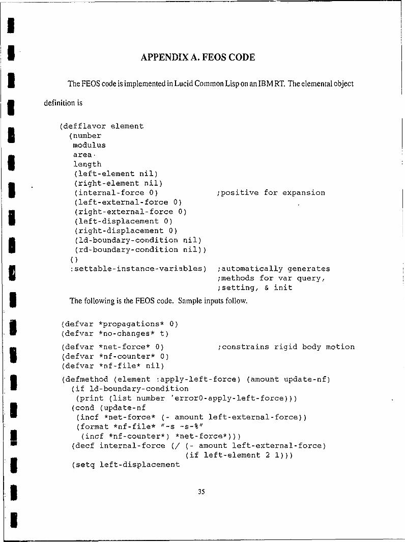
I APPENDIX A. FEOS CODE

I The FEOS code is implemented in Lucid Common Lisp on an IBM RT. The elemental object

U definition is

(defflavor element(numbermodulusarea.length(left-element nil)(right-element nil)(internal-force 0) ;positive for expansion(left-external-force 0)(right-external-force 0)(left-displacement 0)(right-displacement 0)(!d-boundary-condition nil)(rd-boundary-condition nil))

():settable-instance-variables) ;automatically generates

;methods for var query,;setting, & init

3 The following is the FEOS code. Sample inputs follow.

(defvar *propagations* 0)(defvar *no-changes* t)

(defvar *net-force* 0) ;constrains rigid body motion3 (defvar *nf-counter* 0)(defvar *nf-file* nil)

(defmethod (element :apply-left-force) (amount update-nf)(if ld-boundary-condition(print (list number 'errorO-apply-left-force)))

(cond (update-nf(incf *net-force* (- amount left-external-force))(format *nf-file* "-s -s-%"(incf *nf-counter*) *net-force*)))

(decf internal-force (/ (- amount left-external-force)(if left-element 2 1)))3 (setq left-displacement

135

I

(- right-displacement (/ (* length internal-force)area modulus)))

(setq left-external-force amount)(cond((not right-element)(incf *net-force* (- internal-force right-external-force))(format *nf-file* "-s -s-%"(incf *nf-counter*) *net-force*)

(setq right-external-force internal-force))))

(defmethod (element :apply-right-force) (amount update-nf)

(if rd-boundary-condition(print (list 'number 'errorO-apply-right-force)))

(cond (update-nf(incf *net-force* (- amount right-external-force))(format *nf-file* "-s -s-%"(incf *nf-counter*) *net-force*)))

(incf internal-force (/ (- amount right-external-force)(if right-element 2 1)))U

(setq right-displacement(+ left-displacement (/ (* length internal-force)

area modulus)))(setq right-external-force amount)(cond((not left-element)(incf *net-force* (- (+ internal-force

left-external-force)))(format *nf-file* "-s -s-%II(incf *nf-counter*) *net-force*)

(setq left-external-force (- internal-force)))))

(defmethod (element :left-guesses) (force displacement)(let* ((k (/ (* area modulus) length))

(displacement-delta (- displacement left-displacement))(force-delta (- (- force internal-force)

left-external-force))(d-disparity (> (abs displacement-delta) d-threshold))(f-disparity (> (abs force-delta) f-threshold))discrepancy)(cond((and ld-boundary-condition d-disparity)(print (list number 'errorO-left-guesses)))

((and Id-boundary-condition f-disparity)(send self :inc-lef force-delta)(setq *no-changes* nil))

36

I

I ((and d-disparity f-disparity)(let ((delta (/ (- force-delta (* k displacement-delta))

2)))(incf internal-force delta)(if rd-boundary-condition

(send self :inc-ref delta))(decf left-displacement (/ delta k)))

(setq *no-changes* nil))((and d-disparity rd-boundary-condition)(incf left-displacement (/ displacement-delta 2))(decf internal-force (/ (* k displacement-delta) 2))(send self :inc-ref (- (/ (* k displacement-delta) 2)))(setq *no-changes* nil))

(d-disparity3 (incf left-displacement (/ displacement-delta 2))(decf right-displacement (/ displacement-delta 4))(decf internal-force (/ (* k displacement-delta) 4))(setq *no-changes* nil))

((and f-disparity rd-boundary-condition)(incf internal-force (/ force-delta 2))(send self :inc-ref (/ force-delta 2))(decf left-displacement (/ force-delta (* 2 k)))(setq *no-changes* nil))

(f-disparity(incf internal-force (/ force-delta 2))(decf left-displacement (/ force-delta (* 4 k)))(incf right-displacement (/ force-delta (* 4 k)))(setq *no-changes* nil))

((> (abs (setq discrepancy(- internal-force

(* k (- right-displacement left-displacement)))))f-threshold)

(decf internal-force discrepancy)(if ld-boundary-condition

(send self :inc-lef (- discrepancy)))(if rd-boundary-condition(send self :inc-ref discrepancy))))))

3(defmethod (element :right-guesses) (force displacement)(let* ((k (/ (* area modulus) length))

(displacement-delta (- displacement right-displacement))(force-delta (- (- internal-force force)

right-external-force))

5 (d-disparity (> (abs displacement-delta) d-threshold))

!37

I(f-disparity (> (abs force-delta) f-threshold))discrepancy)(cond((and d-disparity rd-boundary-condition)(print (list number 'errorO-right-guesses)))

((and f-disparity rd-boundary-condition)(send self :inc-ref force-delta) I(setq *no-changes* nil))((and d-disparity f-disparity)(let ((delta (/ (- (* k displacement-delta) force-delta) U

2)))(incf internal-force delta)(if ld-boundary-condition .(send self :inc-lef (- delta)))

(incf right-displacement (/ delta k)))(setq *no-changes* iil))

((and d-disparity ld-boundary-condition)(incf right-displacement (/ displacement-delta 2))(incf internal-force (/ (* k displacement-delta) 2))(send self :inc-lef (- (/ (* k displacement-delta) 2)))(setq *no-changes* nil))

(d-disparity(incf right-displacement (/ displacement-delta 2))(decf left-displacement (/ displacement-delta 4;)(incf internal-force (/ (* k displacement-delta) 4))(setq *no-changes* nil))

((and f-disparity ld-boundary-condition) I(decf internal-force (/ force-delta 2))

(send self :inc-lef (/ force-delta 2))(decf right-displacement (/ force-delta (* 2 '. I(setq *no-changes* nil))

(f-disparity(decf internal-force (/ force-delta 2))(decf right-displacement (/ force-delta (* 4 k)))(incf left-displacement (/ force-delta (* 4 k)))(setq *no-changes* nil)) U

((> (abs (setq discrepancy(- internal-force

(* k (- right-displacement left-displacement)))))f-threshold)

(decf internal-force discrepancy) 3(if rd-boundary-condition(send self :inc-ref discrepancy))

38

U

(if id-boundary-condition(send self :inc-lef (- discrepancy)))))))

(defmethod (element :inc-lef) (amount)(incf left-external-force amount)(incf *net-force* amount)(format *nffile* "-s -s-%" (incf *nf-counter*) *net-force*)(if left-element

(send left-element :set-right-external-force3 left-external-force)))

(defmethod (element :inc-ref) (amount)(incf right-external-force amount)

(incf *net-force* amount)(format *nf-file* "-s -s-%" (incf *nf-counter*) *net-force*)(if right-element

(send right-element :set-left-external-forceright-external-force)))

5 (defmethod (element :propagate-left) ()(cond(left-element(incf *propagations*)(send left-element :right-guesses

internal-force left-displacement))))

(defmethod (element :propagate-right) ()(cond(right-element(incf *propagations*)(send right-element :left-guesses3 internal-force right-displacement))))

(defmethod (element :output) ()(format t "-%Element -s:-%external-

forces: left: -s right: -s-%internal-force: -s-%displace-ments: left: -s right: -s-%"

number left-external-force right-external-forceinternal-force left-displacement right-displacement))

(defmethod (element :satisfies-constraints) ()(<- internal-force

(* (/ (* area modulus) length)(- right-displacement left-displacement)))

f-threshold))

(defun calculate (elements)3 (let (mesh

3

I(iterations 0)(start-time (get-internal-run-time)))

(setq *propagations* 0)(if *nf-file* (close *nf-file*)) I(setf *nf-file* (open "nf"

:direction :output:if-exists :rename)) 3

(setf *nf-counter* 0)(setq *net-force* 0)(format *nf-file* -s -s-%"

(incf *nf-counter*) *net-force*)(if (satisfies-constraints

(setq mesh (generate-mesh (rest elements)))(if (satisfies-constraints(output-mesh(progn(format t "-%Mesh initially stable")(format t "-%Calculating -s element mesh"

(list-length mesh))(setq *no-changes* nil)(loop (incf iterations)(if (= (truncate (/ iterations 5)) (/ iterations 5))

(format t "."))(setq *no-changes* t)(dolist (element mesh)

(send element :propagate-left)(send element :propagate-right))

(if *no-changes* (return mesh))))))(format t "-%Solution satisfies constraints") 2

(formatt i"-%Solution does not satisfy constraints"))

(format t "-%Mesh initially unstable"))(format t "-%Net force: -s" *net-force*)(format t "-%Elaspsed time: -s"

(time-since start-time))(format t "-%Propagations: -s" *propagations*)(format t "-%Iterations: -s" iterations)(close *nf-file*)))

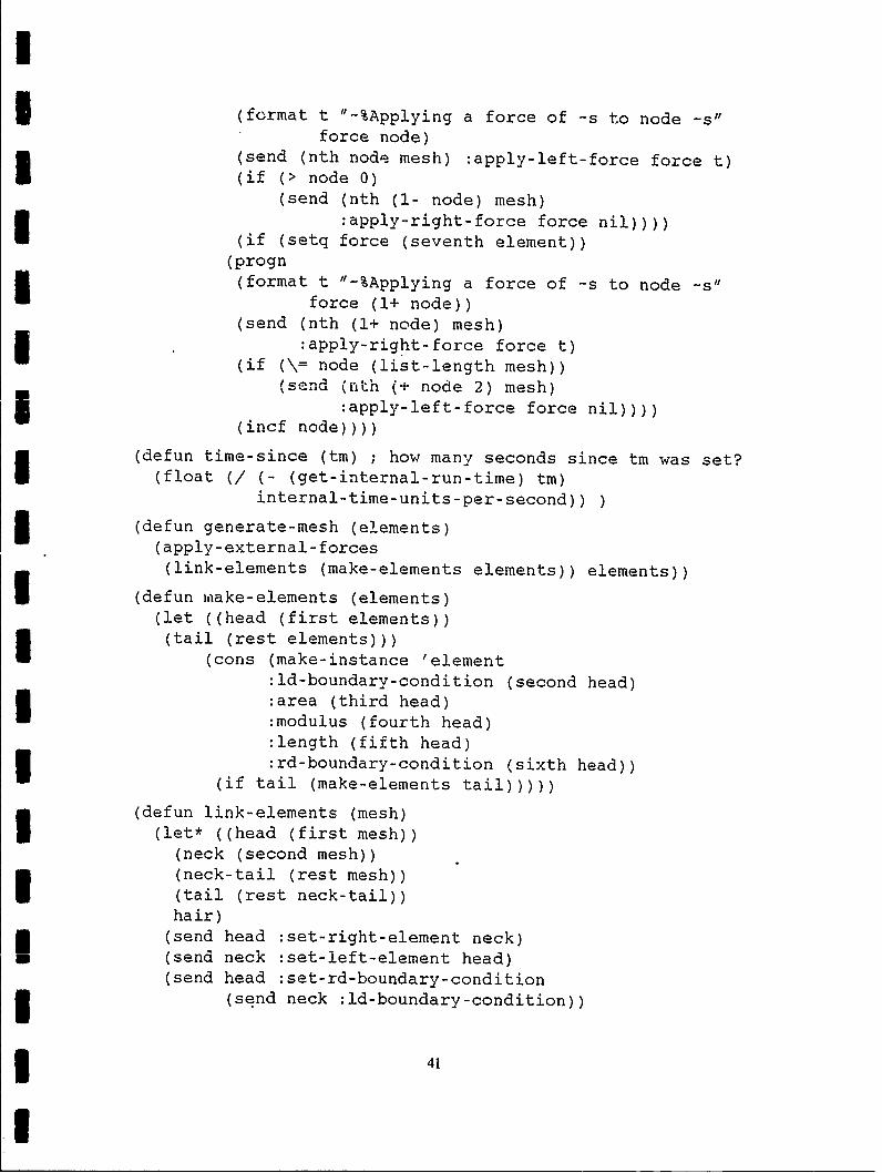
(defun apply-external-forces (mesh elements)(let (force (node 0))

(dolist (element elements mesh)(if (setq force (first element))

(progn

40

I

3 (format t "-%Applying a force of -s to node -s"force node)

(send (nth node mesh) :apply-left-force force t)(if (> node 0)

(send (nth (1- node) mesh):apply-right-force force nil))))

(if (setq force (seventh element))(progn(format t "-%Applying a force of -s to node -s"

force (1+ node))(send (nth (1+ node) mesh)

:apply-right-force force t)(if (\= node (list-length mesh))

( se n d (nLh (+ node 2) mesh):apply-left-force force nil))))

(incf node))))

(defun time-since (tm) ; how many seconds since tm was set?(float (/ (- (get-internal-run-time) tm)

internal-time-units-per-second))

(defun generate-mesh (elements)(apply-external-forces(link-elements (make-elements elements)) elements))

I (defun make-elements (elements)(let ((head (first elements))(tail (rest elements)))

(cons (make-instance 'element:ld-boundary-condition (second head):area (third head):modulus (fourth head):length (fifth head):rd-boundary-condition (sixth head))

(if tail (make-elements tail)))))

(defun link-elements (mesh)(let* ((head (first mesh))

(neck (second mesh))(neck-tail (rest mesh))(tail (rest neck-tail))hair)3 (send head :set-right-element neck)

w (send neck :set-left-element head)(send head :set-rd-boundary-condition3 (send neck :ld-boundary-condition))

341

I(if (setq hair (send head :left-element))

(send head :set-number (1+ (send hair :number))) I(send head :set-number 0))

(if tail(link-elements neck-tail)(send neck :set-number (1+ (send head :number))))

mesh)) 3(defun output-mesh (mesh)

(let ((tail (rest mesh)))(send (first mesh) :output)(if tail (output-mesh tail))mesh))

(defun satisfies-constraints (mesh)(let ((result t))

(dolist (element mesh result) 3(if (not (send element :satisfies-constraints))

(setq result nil)))))

The following is a sample input Example 3.1 from Logan [Logan86].

(defconstant d-threshold 0.00001) 3(defconstant f-threshold 1)

; Problems are input as a list whose first member is a list; of the compression/expansion states of the problem elements Iand the rest of the list is elements. Each element is alist of its features in the following order:left-external-force ld-boundary-conditionarea modulus lengthrd-boundary-condition right-external-force nAny properties not needed at the end are accepted as nil.

(defun eg3.1 ()'((e c c r 1 l)(nil t 1 30E6 30) I

(3000 nil 1 30E6 30)(nil nil 2 15E6 30 t))) 3

4

42

U

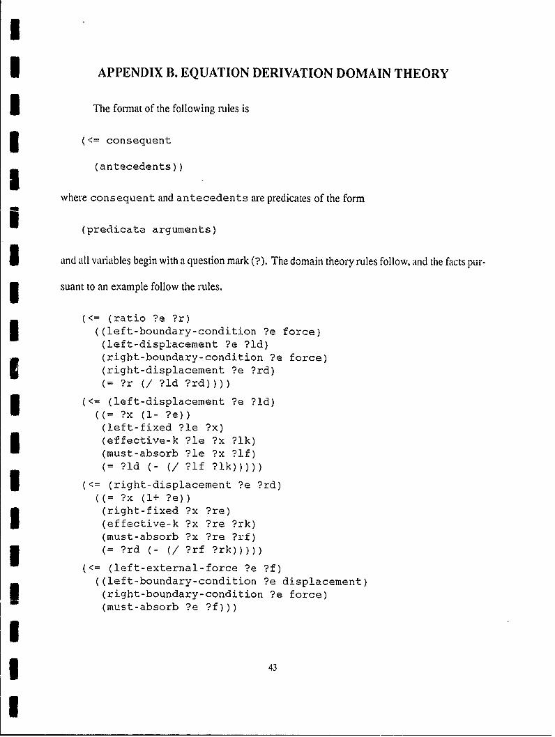
U APPENDIX B. EQUATION DERIVATION DOMAIN THEORY

1 The format of the following rules is

3 (<= consequent

(antecedents))

where consequent and antecedents are predicates of the form

1 (predicate arguments)

I and all variables begin with a question mark (?). The domain theory rules follow, and the facts pur-

3 suant to an example follow the rules.

(<= (ratio ?e ?r)((left-boundary-condition ?e force)(left-displacement ?e ?ld)(right-boundary-condition ?e force)(right-displacement ?e ?rd)(= ?r (/ ?ld ?rd))))

(<= (left-displacement ?e ?ld)((= ?x (1- ?e))(left-fixed ?le ?x)(effective-k ?le ?x ?lk)(must-absorb ?le ?x ?If)(= ?id (- (/ ?if ?ik)))))

3 (<= (right-displacement ?e ?rd)((= ?x (1+ ?e))(right-fixed ?x ?re)(effective-k ?x ?re ?rk)(must-absorb ?x ?re ?rf)3 (= ?rd (- (/ ?rf ?rk)))))

(<= (left-external-force ?e ?f)((left-boundary-condition ?e displacement)(right-boundary-condition ?e force)(must-absorb ?e ?f)))

4* 4

I

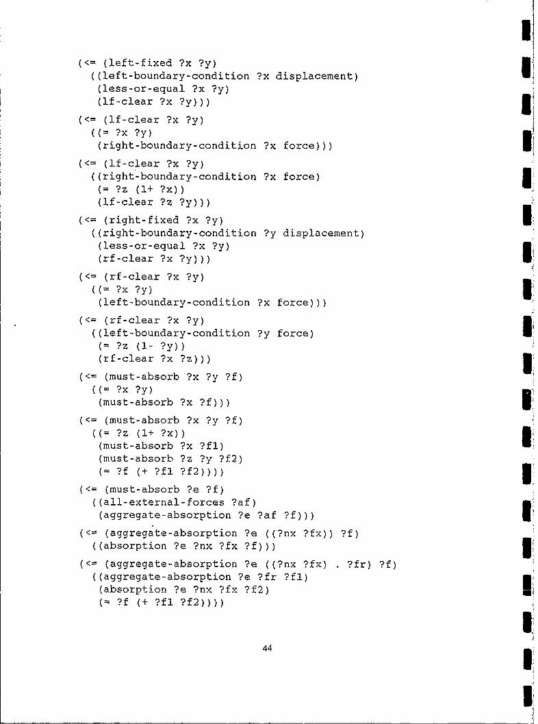
( left-fixed ?x ?y)((left-boundary-condition ?x displacement) U.(less-or-equal ?x ?y)(lf-clear ?x ?y))) I

(<= (lf-clear ?x ?y)((= ?x ?y)(right-boundary-condition ?x force)))

(<= (if-clear ?x ?y)((right-boundary-condition ?x force)(= ?z (1+ ?x))(lf-clear ?z ?y)))

(<= (right-fixed ?x ?y)((right-boundary-condition ?y displacement)(less-or-equal ?x ?y)(rf-clear ?x ?y)))

(<= (rf-clear ?x ?y)

((= ?x ?y)(left-boundary-condition ?x force)))

(<= (rf-clear ?x ?y)((left-boundary-condition ?y force)(= ?z (1- ?y))(rf-clear ?x ?z)))

(<= (must-absorb ?x ?y ?f)((= ?x ?y)(must-absorb ?x ?f)))(must-absorb ?x ?y ?f)

((= ?z (1+ ?x))(must-absorb ?x ?fl)(must-absorb ?z ?y ?f2)

(= ?f (+ ?fl ?f2))))

(<= (must-absorb ?e ?f)((all-external-forces ?af)(aggregate-absorption ?e ?af ?f)))

(<= (aggregate-absorption ?e ((?nx ?fx)) ?f)((absorption ?e ?nx ?fx ?f)))

(<= (aggregate-absorption ?e ((?nx ?fx) ?fr) ?f)((aggregate-absorption ?e ?fr ?fl)(absorption ?e ?nx ?fx ?f2)(= ?f (+ ?fl ?f2))))

44

3 (<= (absorption ?e ?n ?ef 0)((less ?e ?n) ;?e left of ?n(= ?x (1- ?n))(left-fixed ?le ?x)(less ?e ?le)))

(<= (absorption ?e ?n ?ef ?f)((less ?e ?n) ;left

( ?x (1- ?n))(left-fixed ?le ?x)(less-or-equal ?le ?e)(side-share ?le ?x ?n ?ef ?sf)(element-share ?e ?le ?x ?sf ?f)))

(<= (absorption ?e ?n ?ef 0)((less-or-equal ?n ?e) ;right(right-fixed ?n ?re)(less ?re ?e)))

3 (<= (absorption ?e ?n ?ef ?f)((less-or-equal ?n ?e) ;right(right-fixed ?n ?re)(less-or-equal ?e ?re)(side-share ?n ?re ?n ?ef ?sf)(element-share ?e ?n ?re ?sf ?f)))

(<= (side-share ?le ?x ?n ?ef ?sh)((less ?le ?n) ;left(effective-k ?le ?x ?lk)(right-fixed ?n ?re)(effective-k ?n ?re ?rk)(= ?sh (* (/ ?lk (+ ?lk ?rk)) (- ?ef)))))

(<= (side-share ?y ?re ?n ?ef ?sh) ;right((= ?y ?n)

(effective-k ?y ?re ?rk)(= ?z (1- ?y))(left-fixed ?x ?i)(effective-k ?x ?z ?lk)(= ?sh (* (/ ?lk (+ ?lk ?rk)) (- ?ef)))))

3 (<= (effective-k ?x ?y ?k)((= ?x ?y)(value ?x k ?k)))

(<= (effective-k ?x ?y ?k)((e-k ?x ?y ?l ?k)))

I

I 4

U(<= (e-k ?x ?y ?l ?k) 3

((= ?x ?y)(value ?x k ?k)(value ?x 1 ?1))) 3

(< (e-k ?x ?y ?1 ?k)((value ?x k ?kl)(value ?x 1 ?11)(= ?re (1+ ?x))(e-k ?re ?y ?lr ?kr)

Sl (+ ?11 ?ir))(= ?k (/ (+ (* ?ii ?11 ?kl) (* ?lr ?lr ?kr))((+ ?11 ?ir) (+ ?11 ?ir))))))n

(<= (element-share ?e ?x ?y ?tf ?f)

((= ?e ?x)(= ?e ?y) i(= ?f ?tf)))

(<= (element-share ?e ?x ?y ?tf ?f)

((= ?e ?x)( ?z (1+ ?e))(effective-k ?z ?y ?rk)(value ?e k ?ek) I(= ?f (* (/ ?ek (+ ?ek ?rk)) ?tf))))

(<= (element-share ?e ?x ?y ?tf ?f) 3((= ?e ?y)(= ?z (I- ?e))

(effective-k ?x ?z ?lk)I(value ?e k ?ek)(= ?f (* (/ ?ek (+ ?ek ?1k)) ?tf))))

(<= (element-share ?e ?x ?y ?tf ?f)(= ?zl (1- ?e))

=?z2 (1+ ?e))

(effective-k ?x ?zl ?lk)

(effective-k ?z2 ?y ?rk)(value ?e k ?ek)( ?f (* (/ ?ek (+ ?lk ?ek ?rk)) ?tf))))

The following is a set of facts that describe example 3.1 from Logan [Logan86] shown in 3Figure 11.

(all-external-forces ((1 3000.0)))(number-of-elements 3)

46

I

(value 0 k 1.0e6)(value 0 1 30.0)(left-boundary-condition 0 displacement)(right-boundary-condition 0 force)(value 1 k 1.0e6)(value 1 1 30.0)(left-boundary-condition 1 force)(right-boundary-condition 1 force)(value 2 k 1.0e6)(value 2 1 30.0)(left-boundary-condition 2 force)3 (right-boundary-condition 2 displacement)

IIiUI

I

IIUi

I

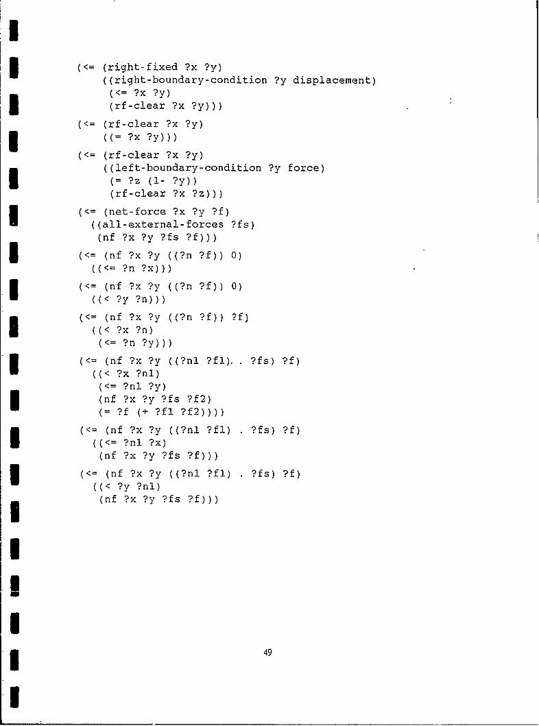
APPENDIX C. QUALITATIVE STATE DOMAIN THEORY i

The format of the following rules is the same as those in APPENDIX B.

(<= (ce-state ?e expansion)((left-fixed ?le ?e)1(net-force ?le ?e 0)(right-fixed ?e ?re)(net-force ?e ?re ?fr)(< 0 ?fr)))

(<= (ce-state ?e compression) 3((left-fixed ?le ?e)(net-force ?le ?e 0)(right-fixed ?e ?re)(net-force ?e ?re ?fr)(< ?fr 0))) II

(<= (ce-state ?e expansion)((right-fixed ?e ?re)(net-force ?e ?re 0)(left-fixed ?le ?e)(net-force ?le ?e ?fl)(< ?fl 0)))

(<= (ce-state ?e compression)((right-fixed ?e ?re)(net-force ?e ?re 0)(left-fixed ?le ?e)(net-force ?le ?e ?fl)(< 0 ?fl)))

(<= (left-fixed ?x ?y)((left-boundary-condition ?x displacement)(<= ?x ?y)(if-clear ?x ?y)))

(<= (if-clear ?x ?y)((= ?X ?y)))

(<= (if-clear ?x ?y)((right-boundary-condition ?x force)

(= ?z (1+ ?x))(if-clear ?z ?y)))I

48

(=(right-fixed ?x ?y)((right-boundary-condition ?y displacement)

(<= ?x ?y)1r-la ? y)(rf-clear ?x ?y))

3 ((= ?x ?y))

(< (rf-clear ?x ?y)((left-boundary-condition ?y force)I (= ?z (1- ?y))(rf-clear ?x ?z)))

(=(net-force ?x ?y ?f)((all-external-forces ?fs)(nf ?x ?y ?fs ?f)))

3 (<=(nf ?x ?y ((?n ?f)) 0)

(=(nf ?x ?y ((?n ?f)) 0)I ((< ?y ?n)))

(=(nf ?x ?y ((?n ?f)) ?f)I ((<?x ?n)(=?n ?y)))

In x? (n f).?s f(<?x ?nl)(=?nJ. ?y)3 (nf ?x ?y ?fs ?f2)

(= ?f (+ ?fl ?f2))))

(< (nf ?x ?y ((?nl ?fl) ?fs) ?f)((<= ?nl ?x)(nf ?x ?y ?fs ?f)))

3 ((=(nf ?x ?y (('?nl ?fl) ?fs) ?f)((< ?y ?nl)(nf ?x ?y ?fs ?f)))

I 49

IREFERENCES

[Abelson89] H. Abelson, M. Eisenberg, M. Halfant, J. Katzenelson, E. Sacks, G. Sussman, J.Wisdom and K. Yip, "Intelligence in Scientific Computing," Communications ofthe Association for Computing Machinery 32, (May 1989), pp. 546-562. 1

[DeJong86] G. F. DeJong and R. J. Mooney, "Explanation-Based Learning: An AlternativeView," Machine Learning 1,2 (April 1986), pp. 145-176. (Also appears as Tech-nical Report UILU-ENG-86-2208, Al Research Group, Coordinated ScienceLaboratory, University of Illinois at Urbana-Champaign.)

[Forbus84] K. D. Forbus, "Qualitative Process Theory," Artificial Intelligence 24, (1984), 3pp. 85-168.

[LaLonde90] W. R. LaLonde and J. R. Pugh, Inside Smalltalk, Prentice Hall, 1990. 3[Logan86] D. L. Logan, A First Course in the Finite Element Method, PWS-Kent, Boston,

1986. 3[Minton89] S. Minton, J. G. Carbonell, C. A. Knoblock, D. R. Kuokka, 0. Etzioni and Y. Gil,

"Explanation-Based Learning: A Problem Solving Perspective," Artificial Intel-ligence 40, (1989), pp. 63-118. I

[Mitchell86] T. M. Mitchell, R. Keller and S. Kedar-Cabelli, "Explanation-Based General-ization: A Unifying View," Machine Learning 1, 1 (January 1986), pp. 47-80.

[Mooney86] R. J. Mooney and S. W. Bennett, "A Domain Independent Explanation-BasedGeneralizer," Proceedings of the National Conference on Artificial Intelligence,Philadelphia, PA, August 1986, pp. 55 1- 5 5 5 . (Also appears as Technical Report UUILU-ENG-86-2216, Al Research Group, Coordinated Science Laboratory,University of Illinois at Urbana-Champaign.)

[Simmons86] R. Simmons, "'Commonsense' Arithmetic Reasoning," Proceedings of the Na-tional Conference on Artificial Intelligence, Philadelphia, PA, August 1986, pp.118-124. 3

IIIUU

50 II