Embed Size (px)
Citation preview

Contents
I Probability Review 1
1 Probability Basics 31.1 Functions and moments . . . . . . . . . . . . . . . . . . . . . . . . . . . . . . . . . . . . . . . . 31.2 Percentiles . . . . . . . . . . . . . . . . . . . . . . . . . . . . . . . . . . . . . . . . . . . . . . . 41.3 Conditional probability and expectation . . . . . . . . . . . . . . . . . . . . . . . . . . . . . . . 61.4 Probability distributions . . . . . . . . . . . . . . . . . . . . . . . . . . . . . . . . . . . . . . . . 8
Exercises . . . . . . . . . . . . . . . . . . . . . . . . . . . . . . . . . . . . . . . . . . . . . . . 9Solutions . . . . . . . . . . . . . . . . . . . . . . . . . . . . . . . . . . . . . . . . . . . . . . . 12
2 Variance 192.1 Additivity . . . . . . . . . . . . . . . . . . . . . . . . . . . . . . . . . . . . . . . . . . . . . . . 192.2 Normal approximation . . . . . . . . . . . . . . . . . . . . . . . . . . . . . . . . . . . . . . . . 202.3 Mixtures . . . . . . . . . . . . . . . . . . . . . . . . . . . . . . . . . . . . . . . . . . . . . . . . 212.4 Bernoulli shortcut . . . . . . . . . . . . . . . . . . . . . . . . . . . . . . . . . . . . . . . . . . . 232.5 Conditional variance . . . . . . . . . . . . . . . . . . . . . . . . . . . . . . . . . . . . . . . . . 24
Exercises . . . . . . . . . . . . . . . . . . . . . . . . . . . . . . . . . . . . . . . . . . . . . . . 24Solutions . . . . . . . . . . . . . . . . . . . . . . . . . . . . . . . . . . . . . . . . . . . . . . . 29
II Life Contingencies 33
3 Survival Distributions: Probability Functions, Life Tables 353.1 Probability Functions . . . . . . . . . . . . . . . . . . . . . . . . . . . . . . . . . . . . . . . . . 353.2 Life Tables . . . . . . . . . . . . . . . . . . . . . . . . . . . . . . . . . . . . . . . . . . . . . . 37
Exercises . . . . . . . . . . . . . . . . . . . . . . . . . . . . . . . . . . . . . . . . . . . . . . . 38Solutions . . . . . . . . . . . . . . . . . . . . . . . . . . . . . . . . . . . . . . . . . . . . . . . 42
4 Survival Distributions: Force of Mortality 45Exercises . . . . . . . . . . . . . . . . . . . . . . . . . . . . . . . . . . . . . . . . . . . . . . . 50Solutions . . . . . . . . . . . . . . . . . . . . . . . . . . . . . . . . . . . . . . . . . . . . . . . 57
5 Survival Distributions: Mortality Laws 655.1 Mortality Laws for Exam Questions . . . . . . . . . . . . . . . . . . . . . . . . . . . . . . . . . 65
5.1.1 Exponential Distribution, or Constant Force of Mortality . . . . . . . . . . . . . . . . . . 655.1.2 Uniform Distribution, or de Moivre’s Law . . . . . . . . . . . . . . . . . . . . . . . . . . 665.1.3 Beta Distribution, or Generalized de Moivre’s law . . . . . . . . . . . . . . . . . . . . . 66
5.2 Mortality Laws that May be Used for Human Mortality . . . . . . . . . . . . . . . . . . . . . . . 675.2.1 Gompertz’s Law . . . . . . . . . . . . . . . . . . . . . . . . . . . . . . . . . . . . . . . 675.2.2 Makeham’s Law . . . . . . . . . . . . . . . . . . . . . . . . . . . . . . . . . . . . . . . 675.2.3 Weibull Distribution . . . . . . . . . . . . . . . . . . . . . . . . . . . . . . . . . . . . . 67Exercises . . . . . . . . . . . . . . . . . . . . . . . . . . . . . . . . . . . . . . . . . . . . . . . 67Solutions . . . . . . . . . . . . . . . . . . . . . . . . . . . . . . . . . . . . . . . . . . . . . . . 69
6 Survival Distributions: Moments 73
SOA MLC Study Manual—7th editionCopyright©2008 ASM
iii

iv CONTENTS
6.1 Complete . . . . . . . . . . . . . . . . . . . . . . . . . . . . . . . . . . . . . . . . . . . . . . . 736.2 Curtate . . . . . . . . . . . . . . . . . . . . . . . . . . . . . . . . . . . . . . . . . . . . . . . . . 76
Exercises . . . . . . . . . . . . . . . . . . . . . . . . . . . . . . . . . . . . . . . . . . . . . . . 79Solutions . . . . . . . . . . . . . . . . . . . . . . . . . . . . . . . . . . . . . . . . . . . . . . . 85
7 Survival Distributions: Percentiles, Recursions, and Life Table Concepts 937.1 Percentiles . . . . . . . . . . . . . . . . . . . . . . . . . . . . . . . . . . . . . . . . . . . . . . . 937.2 Recursive Formulas for Life Expectancy . . . . . . . . . . . . . . . . . . . . . . . . . . . . . . . 937.3 Central Death Rate, Lx, Tx, a(x) . . . . . . . . . . . . . . . . . . . . . . . . . . . . . . . . . . . 94
Exercises . . . . . . . . . . . . . . . . . . . . . . . . . . . . . . . . . . . . . . . . . . . . . . . 97Solutions . . . . . . . . . . . . . . . . . . . . . . . . . . . . . . . . . . . . . . . . . . . . . . . 103
8 Survival Distributions: Fractional Ages 1118.1 Uniform Distribution of Deaths . . . . . . . . . . . . . . . . . . . . . . . . . . . . . . . . . . . . 1118.2 Constant Force of Mortality . . . . . . . . . . . . . . . . . . . . . . . . . . . . . . . . . . . . . . 1158.3 Hyperbolic Assumption . . . . . . . . . . . . . . . . . . . . . . . . . . . . . . . . . . . . . . . . 1178.4 Summary . . . . . . . . . . . . . . . . . . . . . . . . . . . . . . . . . . . . . . . . . . . . . . . 120
Exercises . . . . . . . . . . . . . . . . . . . . . . . . . . . . . . . . . . . . . . . . . . . . . . . 121Solutions . . . . . . . . . . . . . . . . . . . . . . . . . . . . . . . . . . . . . . . . . . . . . . . 130
9 Survival Distributions: Select Mortality 141Exercises . . . . . . . . . . . . . . . . . . . . . . . . . . . . . . . . . . . . . . . . . . . . . . . 144Solutions . . . . . . . . . . . . . . . . . . . . . . . . . . . . . . . . . . . . . . . . . . . . . . . 151
10 Insurance: Payable at Moment of Death—Moments—Part 1 15910.1 Definitions and General Formulas . . . . . . . . . . . . . . . . . . . . . . . . . . . . . . . . . . 15910.2 Constant Force of Mortality . . . . . . . . . . . . . . . . . . . . . . . . . . . . . . . . . . . . . . 161
Exercises . . . . . . . . . . . . . . . . . . . . . . . . . . . . . . . . . . . . . . . . . . . . . . . 164Solutions . . . . . . . . . . . . . . . . . . . . . . . . . . . . . . . . . . . . . . . . . . . . . . . 172
11 Insurance: Payable at Moment of Death—Moments—Part 2 18111.1 de Moivre’s Law . . . . . . . . . . . . . . . . . . . . . . . . . . . . . . . . . . . . . . . . . . . 18111.2 Other Mortality Functions . . . . . . . . . . . . . . . . . . . . . . . . . . . . . . . . . . . . . . 18211.3 Integrating ctne−at . . . . . . . . . . . . . . . . . . . . . . . . . . . . . . . . . . . . . . . . . . . 182
11.3.1∫ ∞
0 tne−atdt . . . . . . . . . . . . . . . . . . . . . . . . . . . . . . . . . . . . . . . . . . 18211.3.2
∫ u0 tne−atdt . . . . . . . . . . . . . . . . . . . . . . . . . . . . . . . . . . . . . . . . . . . 183
11.4 Increasing and Decreasing Insurances . . . . . . . . . . . . . . . . . . . . . . . . . . . . . . . . 18311.5 Variance of Endowment Insurance . . . . . . . . . . . . . . . . . . . . . . . . . . . . . . . . . . 18411.6 Normal Approximation . . . . . . . . . . . . . . . . . . . . . . . . . . . . . . . . . . . . . . . . 185
Exercises . . . . . . . . . . . . . . . . . . . . . . . . . . . . . . . . . . . . . . . . . . . . . . . 186Solutions . . . . . . . . . . . . . . . . . . . . . . . . . . . . . . . . . . . . . . . . . . . . . . . 193
12 Insurance Payable at Moment of Death: Percentiles 203Exercises . . . . . . . . . . . . . . . . . . . . . . . . . . . . . . . . . . . . . . . . . . . . . . . 206Solutions . . . . . . . . . . . . . . . . . . . . . . . . . . . . . . . . . . . . . . . . . . . . . . . 210
13 Insurance Payable at End of Year: Moments 217Exercises . . . . . . . . . . . . . . . . . . . . . . . . . . . . . . . . . . . . . . . . . . . . . . . 220Solutions . . . . . . . . . . . . . . . . . . . . . . . . . . . . . . . . . . . . . . . . . . . . . . . 231
14 Insurance Payable at End of Year: Recursions, Varying 241
SOA MLC Study Manual—7th editionCopyright©2008 ASM

CONTENTS v
14.1 Recursive Formulas . . . . . . . . . . . . . . . . . . . . . . . . . . . . . . . . . . . . . . . . . . 24114.2 Increasing and Decreasing Insurance . . . . . . . . . . . . . . . . . . . . . . . . . . . . . . . . . 242
Exercises . . . . . . . . . . . . . . . . . . . . . . . . . . . . . . . . . . . . . . . . . . . . . . . 245Solutions . . . . . . . . . . . . . . . . . . . . . . . . . . . . . . . . . . . . . . . . . . . . . . . 251
15 Insurance: Discrete to Continuous 259Exercises . . . . . . . . . . . . . . . . . . . . . . . . . . . . . . . . . . . . . . . . . . . . . . . 260Solutions . . . . . . . . . . . . . . . . . . . . . . . . . . . . . . . . . . . . . . . . . . . . . . . 263
16 Annuities: Continuous, Expectation 26716.1 Whole Life Annuity . . . . . . . . . . . . . . . . . . . . . . . . . . . . . . . . . . . . . . . . . . 26816.2 Temporary Life Annuity . . . . . . . . . . . . . . . . . . . . . . . . . . . . . . . . . . . . . . . 27016.3 Deferred Life Annuity . . . . . . . . . . . . . . . . . . . . . . . . . . . . . . . . . . . . . . . . 27116.4 Other Annuities . . . . . . . . . . . . . . . . . . . . . . . . . . . . . . . . . . . . . . . . . . . . 272
16.4.1 n-year certain and life annuity . . . . . . . . . . . . . . . . . . . . . . . . . . . . . . . . 27216.4.2 Accumulated value . . . . . . . . . . . . . . . . . . . . . . . . . . . . . . . . . . . . . . 27216.4.3 Increasing and decreasing annuities . . . . . . . . . . . . . . . . . . . . . . . . . . . . . 272Exercises . . . . . . . . . . . . . . . . . . . . . . . . . . . . . . . . . . . . . . . . . . . . . . . 273Solutions . . . . . . . . . . . . . . . . . . . . . . . . . . . . . . . . . . . . . . . . . . . . . . . 277
17 Annuities: Discrete, Expectation 28317.1 Annuities-due . . . . . . . . . . . . . . . . . . . . . . . . . . . . . . . . . . . . . . . . . . . . . 28317.2 Annuities-immediate . . . . . . . . . . . . . . . . . . . . . . . . . . . . . . . . . . . . . . . . . 28517.3 Accumulated value . . . . . . . . . . . . . . . . . . . . . . . . . . . . . . . . . . . . . . . . . . 287
Exercises . . . . . . . . . . . . . . . . . . . . . . . . . . . . . . . . . . . . . . . . . . . . . . . 289Solutions . . . . . . . . . . . . . . . . . . . . . . . . . . . . . . . . . . . . . . . . . . . . . . . 302
18 Annuities: Variance 313Exercises . . . . . . . . . . . . . . . . . . . . . . . . . . . . . . . . . . . . . . . . . . . . . . . 317Solutions . . . . . . . . . . . . . . . . . . . . . . . . . . . . . . . . . . . . . . . . . . . . . . . 324
19 Annuities: Percentiles, Recursive Calculations 33319.1 Distribution function of annuity random variable . . . . . . . . . . . . . . . . . . . . . . . . . . 33319.2 Percentiles . . . . . . . . . . . . . . . . . . . . . . . . . . . . . . . . . . . . . . . . . . . . . . . 33319.3 Recursive calculations . . . . . . . . . . . . . . . . . . . . . . . . . . . . . . . . . . . . . . . . 335
Exercises . . . . . . . . . . . . . . . . . . . . . . . . . . . . . . . . . . . . . . . . . . . . . . . 336Solutions . . . . . . . . . . . . . . . . . . . . . . . . . . . . . . . . . . . . . . . . . . . . . . . 343
20 Annuities: m-thly Payments 353Exercises . . . . . . . . . . . . . . . . . . . . . . . . . . . . . . . . . . . . . . . . . . . . . . . 354Solutions . . . . . . . . . . . . . . . . . . . . . . . . . . . . . . . . . . . . . . . . . . . . . . . 357
21 Premiums: Fully Continuous Expectation 36121.1 Loss at Issue . . . . . . . . . . . . . . . . . . . . . . . . . . . . . . . . . . . . . . . . . . . . . . 363
Exercises . . . . . . . . . . . . . . . . . . . . . . . . . . . . . . . . . . . . . . . . . . . . . . . 364Solutions . . . . . . . . . . . . . . . . . . . . . . . . . . . . . . . . . . . . . . . . . . . . . . . 368
22 Premiums: Discrete Expectation 37322.1 Three Premium Principle . . . . . . . . . . . . . . . . . . . . . . . . . . . . . . . . . . . . . . . 376
Exercises . . . . . . . . . . . . . . . . . . . . . . . . . . . . . . . . . . . . . . . . . . . . . . . 377Solutions . . . . . . . . . . . . . . . . . . . . . . . . . . . . . . . . . . . . . . . . . . . . . . . 392
SOA MLC Study Manual—7th editionCopyright©2008 ASM

vi CONTENTS
23 Premiums: Percentile of Loss at Issue 409Exercises . . . . . . . . . . . . . . . . . . . . . . . . . . . . . . . . . . . . . . . . . . . . . . . 410Solutions . . . . . . . . . . . . . . . . . . . . . . . . . . . . . . . . . . . . . . . . . . . . . . . 411
24 Premiums: Variance of Loss at Issue, Continuous 415Exercises . . . . . . . . . . . . . . . . . . . . . . . . . . . . . . . . . . . . . . . . . . . . . . . 417Solutions . . . . . . . . . . . . . . . . . . . . . . . . . . . . . . . . . . . . . . . . . . . . . . . 421
25 Premiums: Variance of Loss at Issue, Discrete 429Exercises . . . . . . . . . . . . . . . . . . . . . . . . . . . . . . . . . . . . . . . . . . . . . . . 430Solutions . . . . . . . . . . . . . . . . . . . . . . . . . . . . . . . . . . . . . . . . . . . . . . . 435
26 Premiums: True Fractional Premiums 441Exercises . . . . . . . . . . . . . . . . . . . . . . . . . . . . . . . . . . . . . . . . . . . . . . . 442Solutions . . . . . . . . . . . . . . . . . . . . . . . . . . . . . . . . . . . . . . . . . . . . . . . 444
27 Reserves: Prospective Formula 449Exercises . . . . . . . . . . . . . . . . . . . . . . . . . . . . . . . . . . . . . . . . . . . . . . . 452Solutions . . . . . . . . . . . . . . . . . . . . . . . . . . . . . . . . . . . . . . . . . . . . . . . 457
28 Reserves: Retrospective Formula 46328.1 Three Premium Principle . . . . . . . . . . . . . . . . . . . . . . . . . . . . . . . . . . . . . . . 465
Exercises . . . . . . . . . . . . . . . . . . . . . . . . . . . . . . . . . . . . . . . . . . . . . . . 467Solutions . . . . . . . . . . . . . . . . . . . . . . . . . . . . . . . . . . . . . . . . . . . . . . . 473
29 Reserves: Annuity-Ratio and Insurance-Ratio Formulas 48129.1 Summary of Reserve Formulas . . . . . . . . . . . . . . . . . . . . . . . . . . . . . . . . . . . . 481
Exercises . . . . . . . . . . . . . . . . . . . . . . . . . . . . . . . . . . . . . . . . . . . . . . . 484Solutions . . . . . . . . . . . . . . . . . . . . . . . . . . . . . . . . . . . . . . . . . . . . . . . 492
30 Reserves: Variance of Loss 499Exercises . . . . . . . . . . . . . . . . . . . . . . . . . . . . . . . . . . . . . . . . . . . . . . . 500Solutions . . . . . . . . . . . . . . . . . . . . . . . . . . . . . . . . . . . . . . . . . . . . . . . 504
31 Reserves: Recursive Formulas 509Exercises . . . . . . . . . . . . . . . . . . . . . . . . . . . . . . . . . . . . . . . . . . . . . . . 511Solutions . . . . . . . . . . . . . . . . . . . . . . . . . . . . . . . . . . . . . . . . . . . . . . . 521
32 Reserves: Advanced Topics 53132.1 General Insurances . . . . . . . . . . . . . . . . . . . . . . . . . . . . . . . . . . . . . . . . . . 53132.2 Refund of Reserve . . . . . . . . . . . . . . . . . . . . . . . . . . . . . . . . . . . . . . . . . . 53232.3 Fractional Premiums . . . . . . . . . . . . . . . . . . . . . . . . . . . . . . . . . . . . . . . . . 53432.4 Fractional Durations . . . . . . . . . . . . . . . . . . . . . . . . . . . . . . . . . . . . . . . . . 53532.5 Accounting Loss . . . . . . . . . . . . . . . . . . . . . . . . . . . . . . . . . . . . . . . . . . . 536
Exercises . . . . . . . . . . . . . . . . . . . . . . . . . . . . . . . . . . . . . . . . . . . . . . . 538Solutions . . . . . . . . . . . . . . . . . . . . . . . . . . . . . . . . . . . . . . . . . . . . . . . 546
33 Multiple Lives: Joint Life Probabilities 555Exercises . . . . . . . . . . . . . . . . . . . . . . . . . . . . . . . . . . . . . . . . . . . . . . . 557Solutions . . . . . . . . . . . . . . . . . . . . . . . . . . . . . . . . . . . . . . . . . . . . . . . 561
SOA MLC Study Manual—7th editionCopyright©2008 ASM

CONTENTS vii
34 Multiple Lives: Last Survivor Probabilities 565Exercises . . . . . . . . . . . . . . . . . . . . . . . . . . . . . . . . . . . . . . . . . . . . . . . 568Solutions . . . . . . . . . . . . . . . . . . . . . . . . . . . . . . . . . . . . . . . . . . . . . . . 572
35 Multiple Lives: Moments 575Exercises . . . . . . . . . . . . . . . . . . . . . . . . . . . . . . . . . . . . . . . . . . . . . . . 576Solutions . . . . . . . . . . . . . . . . . . . . . . . . . . . . . . . . . . . . . . . . . . . . . . . 579
36 Multiple Lives: Insurances 585Exercises . . . . . . . . . . . . . . . . . . . . . . . . . . . . . . . . . . . . . . . . . . . . . . . 587Solutions . . . . . . . . . . . . . . . . . . . . . . . . . . . . . . . . . . . . . . . . . . . . . . . 592
37 Multiple Lives: Annuities 597Exercises . . . . . . . . . . . . . . . . . . . . . . . . . . . . . . . . . . . . . . . . . . . . . . . 601Solutions . . . . . . . . . . . . . . . . . . . . . . . . . . . . . . . . . . . . . . . . . . . . . . . 607
38 Multiple Lives: Contingent Survival Functions 61338.1 Contingent Probabilities . . . . . . . . . . . . . . . . . . . . . . . . . . . . . . . . . . . . . . . 61338.2 Contingent Insurances . . . . . . . . . . . . . . . . . . . . . . . . . . . . . . . . . . . . . . . . 617
Exercises . . . . . . . . . . . . . . . . . . . . . . . . . . . . . . . . . . . . . . . . . . . . . . . 618Solutions . . . . . . . . . . . . . . . . . . . . . . . . . . . . . . . . . . . . . . . . . . . . . . . 623
39 Multiple Lives: Common Shock 629Exercises . . . . . . . . . . . . . . . . . . . . . . . . . . . . . . . . . . . . . . . . . . . . . . . 632Solutions . . . . . . . . . . . . . . . . . . . . . . . . . . . . . . . . . . . . . . . . . . . . . . . 634
40 Multi-decrement Models: Probabilities 639Exercises . . . . . . . . . . . . . . . . . . . . . . . . . . . . . . . . . . . . . . . . . . . . . . . 641Solutions . . . . . . . . . . . . . . . . . . . . . . . . . . . . . . . . . . . . . . . . . . . . . . . 648
41 Multi-decrement Models: Forces of Decrement 653Exercises . . . . . . . . . . . . . . . . . . . . . . . . . . . . . . . . . . . . . . . . . . . . . . . 654Solutions . . . . . . . . . . . . . . . . . . . . . . . . . . . . . . . . . . . . . . . . . . . . . . . 660
42 Multi-decrement Models: Associated Single Decrement Tables 66742.1 Single Decrement Rates . . . . . . . . . . . . . . . . . . . . . . . . . . . . . . . . . . . . . . . . 66742.2 Going Between Rates and Probabilities under Uniform Distribution . . . . . . . . . . . . . . . . 669
Exercises . . . . . . . . . . . . . . . . . . . . . . . . . . . . . . . . . . . . . . . . . . . . . . . 672Solutions . . . . . . . . . . . . . . . . . . . . . . . . . . . . . . . . . . . . . . . . . . . . . . . 682
43 Multi-decrement Models: Discrete Insurances and Annuities 693Exercises . . . . . . . . . . . . . . . . . . . . . . . . . . . . . . . . . . . . . . . . . . . . . . . 694Solutions . . . . . . . . . . . . . . . . . . . . . . . . . . . . . . . . . . . . . . . . . . . . . . . 695
44 Multi-decrement Models: Continuous Insurances and Annuities 697Exercises . . . . . . . . . . . . . . . . . . . . . . . . . . . . . . . . . . . . . . . . . . . . . . . 699Solutions . . . . . . . . . . . . . . . . . . . . . . . . . . . . . . . . . . . . . . . . . . . . . . . 707
45 Expenses: Expense Premium and Reserve 71545.1 Expense Premium . . . . . . . . . . . . . . . . . . . . . . . . . . . . . . . . . . . . . . . . . . . 71545.2 Expense Reserve . . . . . . . . . . . . . . . . . . . . . . . . . . . . . . . . . . . . . . . . . . . 71645.3 Variance of Loss . . . . . . . . . . . . . . . . . . . . . . . . . . . . . . . . . . . . . . . . . . . 717
SOA MLC Study Manual—7th editionCopyright©2008 ASM

viii CONTENTS
Exercises . . . . . . . . . . . . . . . . . . . . . . . . . . . . . . . . . . . . . . . . . . . . . . . 719Solutions . . . . . . . . . . . . . . . . . . . . . . . . . . . . . . . . . . . . . . . . . . . . . . . 726
46 Expenses: Policy Fees 735Exercises . . . . . . . . . . . . . . . . . . . . . . . . . . . . . . . . . . . . . . . . . . . . . . . 737Solutions . . . . . . . . . . . . . . . . . . . . . . . . . . . . . . . . . . . . . . . . . . . . . . . 740
47 Expenses: Asset Shares 745Exercises . . . . . . . . . . . . . . . . . . . . . . . . . . . . . . . . . . . . . . . . . . . . . . . 748Solutions . . . . . . . . . . . . . . . . . . . . . . . . . . . . . . . . . . . . . . . . . . . . . . . 753
III Stochastic Processes 757
48 Multi-State Models (Markov Chains): Probabilities 759Exercises . . . . . . . . . . . . . . . . . . . . . . . . . . . . . . . . . . . . . . . . . . . . . . . 766Solutions . . . . . . . . . . . . . . . . . . . . . . . . . . . . . . . . . . . . . . . . . . . . . . . 771
49 Multi-State Models (Markov Chains): Premiums and Reserves 77549.1 Prototype Example . . . . . . . . . . . . . . . . . . . . . . . . . . . . . . . . . . . . . . . . . . 77549.2 Insurances . . . . . . . . . . . . . . . . . . . . . . . . . . . . . . . . . . . . . . . . . . . . . . . 77549.3 Annuities . . . . . . . . . . . . . . . . . . . . . . . . . . . . . . . . . . . . . . . . . . . . . . . 77749.4 Premiums and Reserves . . . . . . . . . . . . . . . . . . . . . . . . . . . . . . . . . . . . . . . . 779
Exercises . . . . . . . . . . . . . . . . . . . . . . . . . . . . . . . . . . . . . . . . . . . . . . . 780Solutions . . . . . . . . . . . . . . . . . . . . . . . . . . . . . . . . . . . . . . . . . . . . . . . 785
50 The Poisson Process: Probabilities of Events 78950.1 Introduction . . . . . . . . . . . . . . . . . . . . . . . . . . . . . . . . . . . . . . . . . . . . . . 78950.2 Probabilities—Homogeneous Process . . . . . . . . . . . . . . . . . . . . . . . . . . . . . . . . 79050.3 Probabilities—Non-Homogeneous Process . . . . . . . . . . . . . . . . . . . . . . . . . . . . . . 791
Exercises . . . . . . . . . . . . . . . . . . . . . . . . . . . . . . . . . . . . . . . . . . . . . . . 793Solutions . . . . . . . . . . . . . . . . . . . . . . . . . . . . . . . . . . . . . . . . . . . . . . . 797
51 The Poisson Process: Time To Next Event 801Exercises . . . . . . . . . . . . . . . . . . . . . . . . . . . . . . . . . . . . . . . . . . . . . . . 804Solutions . . . . . . . . . . . . . . . . . . . . . . . . . . . . . . . . . . . . . . . . . . . . . . . 805
52 The Poisson Process: Thinning 80752.1 Constant Probabilities . . . . . . . . . . . . . . . . . . . . . . . . . . . . . . . . . . . . . . . . . 80752.2 Non-Constant Probabilities . . . . . . . . . . . . . . . . . . . . . . . . . . . . . . . . . . . . . . 809
Exercises . . . . . . . . . . . . . . . . . . . . . . . . . . . . . . . . . . . . . . . . . . . . . . . 810Solutions . . . . . . . . . . . . . . . . . . . . . . . . . . . . . . . . . . . . . . . . . . . . . . . 814
53 The Poisson Process: Sums and Mixtures 81953.1 Sums of Poisson Processes . . . . . . . . . . . . . . . . . . . . . . . . . . . . . . . . . . . . . . 81953.2 Mixtures of Poisson Processes . . . . . . . . . . . . . . . . . . . . . . . . . . . . . . . . . . . . 820
Exercises . . . . . . . . . . . . . . . . . . . . . . . . . . . . . . . . . . . . . . . . . . . . . . . 823Solutions . . . . . . . . . . . . . . . . . . . . . . . . . . . . . . . . . . . . . . . . . . . . . . . 825
54 Compound Poisson Processes 82954.1 Definition and Moments . . . . . . . . . . . . . . . . . . . . . . . . . . . . . . . . . . . . . . . 829
SOA MLC Study Manual—7th editionCopyright©2008 ASM

CONTENTS ix
54.2 Sums of Compound Distributions . . . . . . . . . . . . . . . . . . . . . . . . . . . . . . . . . . 830Exercises . . . . . . . . . . . . . . . . . . . . . . . . . . . . . . . . . . . . . . . . . . . . . . . 831Solutions . . . . . . . . . . . . . . . . . . . . . . . . . . . . . . . . . . . . . . . . . . . . . . . 837
IV Practice Exams 843
1 Practice Exam 1 845
2 Practice Exam 2 853
3 Practice Exam 3 861
4 Practice Exam 4 867
5 Practice Exam 5 875
6 Practice Exam 6 883
7 Practice Exam 7 891
8 Practice Exam 8 899
Appendices 907
A Solutions to the Practice Exams 909Solutions for Practice Exam 1 . . . . . . . . . . . . . . . . . . . . . . . . . . . . . . . . . . . . . . . . 909Solutions for Practice Exam 2 . . . . . . . . . . . . . . . . . . . . . . . . . . . . . . . . . . . . . . . . 918Solutions for Practice Exam 3 . . . . . . . . . . . . . . . . . . . . . . . . . . . . . . . . . . . . . . . . 928Solutions for Practice Exam 4 . . . . . . . . . . . . . . . . . . . . . . . . . . . . . . . . . . . . . . . . 938Solutions for Practice Exam 5 . . . . . . . . . . . . . . . . . . . . . . . . . . . . . . . . . . . . . . . . 948Solutions for Practice Exam 6 . . . . . . . . . . . . . . . . . . . . . . . . . . . . . . . . . . . . . . . . 959Solutions for Practice Exam 7 . . . . . . . . . . . . . . . . . . . . . . . . . . . . . . . . . . . . . . . . 971Solutions for Practice Exam 8 . . . . . . . . . . . . . . . . . . . . . . . . . . . . . . . . . . . . . . . . 980
B Solutions to Old Exams 993B.1 Solutions to CAS Exam 3, Spring 2005 . . . . . . . . . . . . . . . . . . . . . . . . . . . . . . . 993B.2 Solutions to SOA Exam M, Spring 2005 . . . . . . . . . . . . . . . . . . . . . . . . . . . . . . . 997B.3 Solutions to CAS Exam 3, Fall 2005 . . . . . . . . . . . . . . . . . . . . . . . . . . . . . . . . . 1006B.4 Solutions to SOA Exam M, Fall 2005 . . . . . . . . . . . . . . . . . . . . . . . . . . . . . . . . 1010B.5 Solutions to CAS Exam 3, Spring 2006 . . . . . . . . . . . . . . . . . . . . . . . . . . . . . . . 1018B.6 Solutions to CAS Exam 3, Fall 2006 . . . . . . . . . . . . . . . . . . . . . . . . . . . . . . . . . 1024B.7 Solutions to SOA Exam M, Fall 2006 . . . . . . . . . . . . . . . . . . . . . . . . . . . . . . . . 1029B.8 Solutions to CAS Exam 3, Spring 2007 . . . . . . . . . . . . . . . . . . . . . . . . . . . . . . . 1037B.9 Solutions to SOA Exam MLC, Spring 2007 . . . . . . . . . . . . . . . . . . . . . . . . . . . . . 1042B.10 Solutions to CAS Exam 3, Fall 2007 . . . . . . . . . . . . . . . . . . . . . . . . . . . . . . . . . 1050B.11 Solutions to CAS Exam 3L, Spring 2008 . . . . . . . . . . . . . . . . . . . . . . . . . . . . . . . 1054
C Exam Question Index 1057
SOA MLC Study Manual—7th editionCopyright©2008 ASM

x CONTENTS
SOA MLC Study Manual—7th editionCopyright©2008 ASM

Lesson 8
Survival Distributions: Fractional Ages
Reading: Actuarial Mathematics 3.6 or Models for Quantifying Risk (2nd edition) 4.5
Life tables, such as the Illustrative Life Table, list mortality rates (qx) or lives (lx) for integral ages only. Often, it isnecessary to determine lives at fractional ages (like lx+0.5 for x an integer) or mortality rates for fractions of a year.We need some way to interpolate between ages.
There are three commonly used interpolation methods: linear, geometric, and harmonic. We will consider allthree of them. Linear interpolation is usually referred to as uniform distribution of deaths between integral agesor UDD. Geometric interpolation is usually referred to as constant force of mortality between integral ages, andmay also be called exponential interpolation. Harmonic interpolation is referred to as hyperbolic interpolation orBalducci’s hypothesis.
8.1 Uniform Distribution of Deaths
The easiest interpolation method is linear interpolation, or uniform distribution of deaths. This means that thenumber of lives at age x + s, 0 ≤ s ≤ 1, is a weighted average of the number of lives at age x and the number of livesat age x + 1:
lx+s = (1 − s)lx + slx+1 = lx − sdx (8.1)
l100+s
1000
00 1
s
550
The graph of lx+s is a straight line between s = 0 and s = 1 with slope−dx. The graph at the right portrays this for a mortality rate q100 = 0.45 andl100 = 1000.
Using lx+s, we can compute sqx:
sqx = 1 − s px
= 1 − lx+s
lx= 1 − (1 − sqx) = sqx
More generally, for 0 ≤ s + t ≤ 1,
sqx+t = 1 − s px+t = 1 − lx+s+t
lx+t
= 1 − lx − (s + t)dx
lx − tdx=
sdx
lx − tdx=
sqx
1 − tqx
(8.2)
where the last equation was obtained by dividing numerator and denominator by lx. The important point to pick upis that while sqx is the proportion of the year s times qx, sqx+t is not sqx, but is in fact higher than sqx. The numberof lives dying in any amount of time is constant, and since there are fewer and fewer lives as the year progresses, therate of death is in fact increasing over the year. The numerator of sqx+t is the proportion of the year being measureds times the death rate, but then this must be divided by 1 minus the proportion of the year that elapsed before thestart of measurement.
For most problems involving death rates, it will suffice if you remember that lx+s is linearly interpolated. Tryworking out the following example before looking at the answer.
SOA MLC Study Manual—7th editionCopyright©2008 ASM
111

112 8. SURVIVAL DISTRIBUTIONS: FRACTIONAL AGES
EXAMPLE 8A You are given:(i) qx = 0.1
(ii) Uniform distribution of deaths between integral ages is assumed.Calculate 1/2qx+1/4.
ANSWER: Let lx = 1. Then lx+1 = lx(1 − qx) = 0.9 and dx = 0.1. Linearly interpolating,
lx+1/4 = lx − 14 dx = 1 − 1
4 (0.1) = 0.975
lx+3/4 = lx − 34 dx = 1 − 3
4 (0.1) = 0.925
1/2qx+1/4 =lx+1/4 − lx+3/4
lx+1/4=
0.975 − 0.9250.975
= 0.051282 �
You could also use equation (8.2) to work this example.
EXAMPLE 8B For two lives age (x) with independent future lifetimes, k|qx = 0.1(k + 1) for k = 0, 1, 2. Deaths areuniformly distributed between integral ages.
Calculate the probability that both lives will survive 2.25 years.
ANSWER: Since the two lives are independent, the probability of both surviving 2.25 years is the square of 2.25 px,the probability of one surviving 2.25 years. If we let lx = 1 and use dx+k = lx k|qx, we get
qx = 0.1(1) = 0.1 lx+1 = 1 − dx = 1 − 0.1 = 0.9
1|qx = 0.1(2) = 0.2 lx+2 = 0.9 − dx+1 = 0.9 − 0.2 = 0.7
2|qx = 0.1(3) = 0.3 lx+3 = 0.7 − dx+2 = 0.7 − 0.3 = 0.4
Then linearly interpolating between lx+2 and lx+3, we get lx+2.25 = 0.7−0.25(0.3) = 0.625, and 2.25 px =lx+2.25
lx= 0.625.
Squaring, the answer is 0.6252 = 0.390625 . �
µ100+s
s
1
0
0.45
0.450.55
0 1
The conditional density function given survival to x, f (x + s|s ≥ 0) =
s pxµx+s is the constant qx, the derivative of the conditional cumulative distri-bution function sqx = sqx with respect to s. This allows us to derive the forceof mortality:
s pxµx+s = qx (8.3)
µx+s =qx
s px=
qx
1 − sqx(8.4)
The force of mortality increases over the year, as illustrated in the graph to theright for q100 = 0.45.
Under the uniform distribution of deaths hypothesis, the fraction of theyear lived by those dying during the year is a(x) = 1
2 . Therefore, Lx = 12 (lx +
lx+1) and
mx =2dx
lx + lx+1=
qx
1 − 0.5qx(8.5)
Complete Expectation of Life Under UDDIf the complete future lifetime random variable T is written as T = K + S , where K is the curtate future lifetime andS is the fraction of the last year lived, then K and S are independent. This is usually not true if uniform distributionof deaths is not assumed. Since S is uniform on [0, 1), E[S ] = 1
2 and Var(S ) = 112 . It follows from E[S ] = 1
2 that
e̊x = ex + 12 (8.6)
SOA MLC Study Manual—7th editionCopyright©2008 ASM

8.1. UNIFORM DISTRIBUTION OF DEATHS 113
More common on exams are questions asking you to evaluate the temporary complete expectancy of life underUDD. You can always evaluate the temporary complete expectancy, whether or not UDD is assumed, by integratingt px, as indicated by formula (6.4) on page 74. For UDD, t px is linear between integral ages, so evaluating theintegral is particularly easy, as we shall see in the next example.
EXAMPLE 8C You are given(i) qx = 0.1.
(ii) Deaths are uniformly distributed between integral ages.Calculate e̊x:0.4 .
ANSWER: We will discuss two ways to solve this: an algebraic method and a geometric method.The algebraic method uses the fact that for a uniform distribution, the mean is the midpoint. If deaths occur
uniformly between integral ages, that means that those who die within a period contained within a year survive halfthe period on the average.
In this example, those who die within 0.4 survive an average of 0.2. Those who survive 0.4 survive an average of0.4 of course. The temporary life expectancy is the weighted average of these two groups, or 0.4qx(0.2) + 0.4 px(0.4).This is:
0.4qx = (0.4)(0.1) = 0.04
0.4 px = 1 − 0.04 = 0.96
e̊x:0.4 = 0.04(0.2) + 0.96(0.4) = 0.392
An equivalent geometric method is to draw the t px function from 0 to 0.4. The integral of t px is the area underthe line, which is the area of a trapezoid: the average of the heights times the width. The following is the graph (notdrawn to scale):
A B
(0.4, 0.96)(1.0, 0.9)
0 0.4 1.0
1
t px
t
Trapezoid A is the area we are interested in. Its area is 12 (1 + 0.96)(0.4) = 0.392 . �
?Quiz 8-1 1 Once again, you are given
(i) qx = 0.1.(ii) Deaths are uniformly distributed between integral ages.
Calculate e̊x+0.4:0.6 .
Let’s now work out an example where we cross an integral boundary.
EXAMPLE 8D You are given:(i) qx = 0.1
(ii) qx+1 = 0.2(iii) Deaths are uniformly distributed between integral ages.
1Solution is at the end of exercise solutions.
SOA MLC Study Manual—7th editionCopyright©2008 ASM

114 8. SURVIVAL DISTRIBUTIONS: FRACTIONAL AGES
Calculate e̊x+0.5:1 .
ANSWER: Let’s start with the algebraic method. Since the mortality rate changes at x + 1, we must split the groupinto those who die before x + 1, those who die afterwards, and those who survive. Those who die before x + 1 live0.25 on the average since the period to x + 1 is length 0.5. Those who die after x + 1 live between 0.5 and 1 years;the midpoint of 0.5 and 1 is 0.75, so they live 0.75 years on the average. Those who survive live 1 year.
Now let’s calculate the probabilities.
0.5qx+0.5 =0.5(0.1)
1 − 0.5(0.1)=
595
0.5 px+0.5 = 1 − 595
=9095
0.5|0.5qx+0.5 =
(9095
)[0.5(0.2)] =
995
1 px+0.5 = 1 − 595− 9
95=
8195
These probabilities could also be calculated by setting up an lx table with radix 100 at age x and interpolating withinit to get lx+0.5 and lx+1.5. Then
lx+1 = 0.9lx = 90lx+2 = 0.8lx+1 = 72
lx+0.5 = 0.5(90 + 100) = 95lx+1.5 = 0.5(72 + 90) = 81
0.5qx+0.5 = 1 − 9095
=595
0.5|0.5qx+0.5 =90 − 81
95=
995
1 px+0.5 =lx+1.5
lx+0.5=
8195
Either way, we’re now ready to calculate e̊x+0.5:1 .
e̊x+0.5:1 =5(0.25) + 9(0.75) + 81(1)
95=
8995
For the geometric method we draw the following graph:
A B
(0.5, 90
95
)(1.0, 81
95
)
0x + 0.5
0.5x + 1
1.0x + 1.5
1
t px+0.5
t
The heights at x + 1 and x + 1.5 are as we computed above. Then we compute each area separately. The area of A
is 12
(1 + 90
95
)(0.5) = 185
95(4) . The area of B is 12
(9095 + 81
95
)(0.5) = 171
95(4) . Adding them up, we get 185+17195(4) = 89
95 . �
SOA MLC Study Manual—7th editionCopyright©2008 ASM

8.2. CONSTANT FORCE OF MORTALITY 115
?Quiz 8-2 The probability that a battery fails by the end of the kth month is given in the following table:
kProbability of battery failure by the
end of month k1 0.052 0.203 0.60
Between integral months, time of failure for the battery is uniformly distributed.Calculate the expected amount of time the battery survives within 2.25 months.
To calculate e̊x:n for x and n integers in terms of ex:n , note that those who survive n years contribute the same toboth. Those who die contribute an average of 1
2 more to e̊x:n since they die on the average in the middle of the year.Thus the difference is 1
2 nqx:e̊x:n = ex:n + 0.5nqx (8.7)
EXAMPLE 8E Calculate e̊50:10 if qx = 0.01 for 50 < x ≤ 60 and uniform distribution of deaths between integral agesis assumed.
ANSWER: e50:10 is the sum of k p50 = 0.99k, which forms a geometric series:
e50:10 =
10∑
k=1
0.9k =0.99 − 0.9911
1 − 0.99= 9.46617
The probability of dying in 10 years is 1 − 0.9910 = 0.095618. Therefore
e̊50:10 = 9.46617 + 0.5(0.095618) = 9.51398 �
8.2 Constant Force of Mortality
Under constant force of mortality, since in general px = exp(−
∫ 10 µx+sds
)and µx+s = µ is constant,
px = e−µ (8.8)µ = − ln px (8.9)
Moreover, s px = e−µs = psx. In fact, this exponential distribution has no memory, so
s px+t = psx (8.10)
for any 0 ≤ t ≤ 1 − s. Figure 8.1 shows l100+s and µ100+s for l100 = 1000 and q100 = 0.45 if constant force ofmortality is assumed.
As discussed in Section 7.3 in the answer to the third part of Example 7C on page 95, mx = µx if constant forceof mortality is assumed.
We will now repeat some of the previous examples but using constant force of mortality.
EXAMPLE 8F You are given:(i) qx = 0.1
(ii) The force of mortality is constant between integral ages.
SOA MLC Study Manual—7th editionCopyright©2008 ASM

116 8. SURVIVAL DISTRIBUTIONS: FRACTIONAL AGES
l100+s
1000
00 1
s
550
(a) l100+s
µ100+s
s
1
00 1
− ln 0.55 − ln 0.55
(b) µ100+s
Figure 8.1: Example of constant force of mortality
Calculate 1/2qx+1/4.
ANSWER:
1/2qx+1/4 = 1 − 1/2 px+1/4 = 1 − p1/2x = 1 − 0.91/2 = 1 − 0.948683 = 0.051317 �
EXAMPLE 8G You are given:
(i) qx = 0.1(ii) qx+1 = 0.2
(iii) The force of mortality is constant between integral ages.
Calculate e̊x+0.5:1 .
ANSWER: We calculate∫ 1
0 t px+0.5dt. We split this up into 2 integrals, one from 0 to 0.5 for age x and one from 0.5 to1 for age x + 1. The first integral is
∫ 0.5
0t px+0.5dt =
∫ 0.5
0pt
xdt =
∫ 0.5
00.9tdt = −1 − 0.90.5
ln 0.9= 0.487058
For t > 0.5,
t px+0.5 = 0.5 px+0.5 t−0.5 px+1 = 0.90.5t−0.5 px+1
so the second integral is
0.90.5∫ 1
0.5t−0.5 px+1dt = 0.90.5
∫ 0.5
00.8tdt = −
(0.90.5
) (1 − 0.80.5
ln 0.8
)= (0.948683)(0.473116) = 0.448837
The answer is e̊x+0.5:1 = 0.487058 + 0.448837 = 0.935896 . �
Although constant force of mortality is not used as often as UDD, it can be useful for simplifying formulas undercertain circumstances. Calculating the expected present value of an insurance where the death benefit within a yearfollows an exponential pattern (this can happen when the death benefit is the discounted present value of something)may be easier with constant force of mortality than with UDD.
SOA MLC Study Manual—7th editionCopyright©2008 ASM

8.3. HYPERBOLIC ASSUMPTION 117
8.3 Hyperbolic Assumption
Under the hyperbolic assumption,
1lx+s
=1 − s
lx+
slx+1
or
lx+s =lxlx+1
lx+1 + sdx=
lx+1
px + sqx(8.11)
where the last equality is obtained by dividing numerator and denominator by lx. Dividing both sides by lx, we have
s px =px
px + sqx=
px
1 − (1 − s)qx
sqx =sqx
1 − (1 − s)qx(8.12)
More generally,
sqx+t =sqx
1 − [1 − (s + t)]qx(8.13)
Notice that the denominator increases as t increases, so that sqx+t is a decreasing function of age x + t. Not veryplausible, is it.
µx+s is best derived as − dds ln s px, or
µx+s = − dds
ln(
px
1 − (1 − s)qx
)=
qx px(1−(1−s)qx)2
px1−(1−s)qx
=qx
1 − (1 − s)qx(8.14)
and we see that the force of mortality decreases over the year.Figure 8.2 shows l100+s and µ100+s for l100 = 1000 and q100 = 0.45 if a hyperbolic assumption for fractional ages
is assumed.
l100+s
1000
00 1
s
550
(a) l100+s
µ100+s
s
1
00 1
0.450.55
0.45
(b) µ100+s
Figure 8.2: Example of hyperbolic assumption
SOA MLC Study Manual—7th editionCopyright©2008 ASM

118 8. SURVIVAL DISTRIBUTIONS: FRACTIONAL AGES
Calculating mx is messy. First we calculate Lx.
Lx =
∫ 1
0lx+tdt
=
∫ 1
0
lx+1dtpx + tqx
by equation (8.11)
= lx+1ln(px + tqx)
qx
∣∣∣∣∣1
0
= − lx+1 ln px
qx
Then
mx =dx
Lx
= − dxqx
lx px ln px
= − q2x
px ln px
We will now repeat some of the previous examples but using the hyperbolic assumption.
EXAMPLE 8H You are given:(i) qx = 0.1
(ii) Mortality follows the Balducci hypothesis between integral ages.Calculate 1/2qx+1/4.ANSWER:
1/2qx+1/4 =(1/2)qx
1 − [1 − (1/2 + 1/4)]qx=
(0.5)(0.1)1 − 0.25(0.1)
=0.05
0.975= 0.051282
In this case, the answer is the same as with uniform distribution of deaths. �
EXAMPLE 8I You are given:(i) qx = 0.1
(ii) qx+1 = 0.2(iii) Deaths between integral ages follow the hyperbolic assumption.
Calculate e̊x+0.5:1 .
ANSWER: We calculate∫ 1
0 t px+0.5dt. We split this up into 2 integrals, one from 0 to 0.5 for age x and one from 0.5 to1 for age x + 1. By equation (8.13),
s px+t = 1 − sqx
1 − [1 − (s + t)]qx=
1 − (1 − t)qx
1 − [1 − (s + t)]qx
The first integral is∫ 0.5
0t px+0.5 dt =
∫ 0.5
0
(1 − (1 − 0.5)(0.1)
1 − [1 − (0.5 + t)(0.1)]
)dt
=
(0.950.1
)ln{1 − [1 − (0.5 + t)](0.1)}
∣∣∣∣∣∣0.5
0
=
(0.950.1
)(− ln 0.95) = 0.487286
SOA MLC Study Manual—7th editionCopyright©2008 ASM

8.3. HYPERBOLIC ASSUMPTION 119
Under the hyperbolic assumption, 0.5qx+0.5 = 0.5qx, so 0.5 px+0.5 in this example is 1 − 0.5(0.1) = 0.95. For t > 0.5,
t px+0.5 = 0.5 px+0.5 t−0.5 px+1 = 0.95 t−0.5 px+1
so the second integral is (changing the variable, reducing t by 0.5)
0.95∫ 0.5
0t px+1dt = 0.95
∫ 0.5
0
px+1dt1 − (1 − t)qx+1
=
[(0.95)(0.8)
0.2
]ln[1 − (1 − t)(0.2)]
∣∣∣∣∣∣0.5
0
=(0.95)(0.8)(ln 0.9 − ln 0.8)
0.2= 0.471132
The answer is 0.487286 + 0.471132 = 0.934862 �
One convenient thing about the hyperbolic hypothesis is that 1−sqx+s = (1 − s)qx. This can be convenient if theexact starting age at which a population is observed varies within an age.
EXAMPLE 8J A population of 60-year olds with life insurance policies has mortality rate q60 = 0.01. Their birthdaysare uniformly distributed throughout the year.
50 members of this population surrender their contracts on Jan. 1. They are assumed to have randomly dis-tributed birthdays.
Calculate for the 50 lives, as of Jan. 1, the expected number of deaths before their next birthday if:
1. Deaths between integral ages follow the hyperbolic assumption.
2. Deaths between integral ages are uniformly distributed.
ANSWER: 1. The expected number of deaths for each life is (1− s)qx = 0.01(1− s), where 1− s is the amount oftime to the next birthday. We integrate this over the uniform distribution of birthdays (density 1) from 0 to 1,and multiply by 50:
50∫ 1
00.01(1 − s)ds = 0.25
2. The expected number of deaths for each life is 1−sqx+s =(1−s)qx1−sqx
=0.01(1−s)1−0.01s . We integrate this as follows
1 − s1 − 0.01s
= 100 − 991 − 0.01s∫ 1
0
1 − s1 − 0.01s
= 100 − 99∫ 1
0
ds1 − 0.01s
= 100 + 9900 ln(1 − 0.01s)∣∣∣∣1
0
= 100 + 9900 ln 0.99 = 0.501675
Multiplying by 0.01 and by 50 lives, we get 0.5(0.501675) = 0.25084 .The hyperbolic assumption led to an easier calculation. �
The implausible hyperbolic hypothesis is mainly of historical interest. It used to be thought that this hypothesiscould justify a linear method for estimating mortality rates. Because of the awkwardness of the formulas, examquestions have generally been limited to calculating survival probabilities, and on rare occasions force of mortality.
SOA MLC Study Manual—7th editionCopyright©2008 ASM

120 8. SURVIVAL DISTRIBUTIONS: FRACTIONAL AGES
Table 8.1: Summary of formulas for fractional ages
Function Uniform distribution ofdeaths
Constant force of mortality Hyperbolic assumption
lx+s lx − sdx lx psx
lx+1px+sqx
sqx sqx 1 − psx
sqx1−(1−s)qx
sqx+tsqx
1−tqx1 − ps
xsqx
1−[1−(s+t)]qx
µx+sqx
1−sqx− ln px
qx1−(1−s)qx
mxqx
1−0.5qx− ln px − q2
xpx ln px
e̊x ex + 0.5
e̊x:n ex:n + 0.5 (1 − n px)
l100+s
1000
4000 1
s
550
(a) lx+s
µ100+s
s
1
0.40 1
(b) µx+s
LEGENDUniform distribu-tion of deathsConstant force ofmortalityHyperbolicassumption
Figure 8.3: Comparison of the three assumptions for distribution of deaths between integral ages
8.4 Summary
The formulas are summarized in table 8.1. Figure 8.3 compares lx+s and µx+s for the 3 assumptions, using x = 100and qx = 0.45.
What do you need to memorize for the exam? For UDD, if you know the linear formula for lx, you will be ableto answer all probability questions. You will be able to rederive the formula for µx+s, or you may memorize the µx+s
formula.The constant force of mortality appears least often on the released exams, but it is easy. If you know that
s px = e−sµx , you have the whole story.The hyperbolic assumption is the hardest one to memorize, but it is unlikely they will ask anything beyond a
probability question on it. If you memorize the formula for sqx+t, you should be able to get by. To play safe, youmay also memorize the formula for µx+s.
You should also understand the picture, figure 8.3. Namely, UDD kills off lives the slowest, and hyperbolic thefastest. UDD has an increasing force of mortality, and hyperbolic a decreasing force. The constant force of mortalityassumption has a constant force of course, and is in the middle of the other two.
SOA MLC Study Manual—7th editionCopyright©2008 ASM
EXERCISES FOR LESSON 8 121
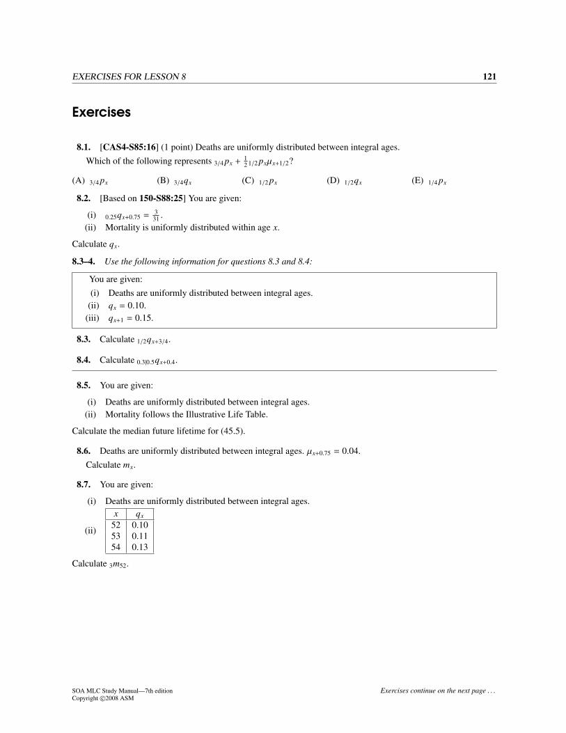
Exercises
8.1. [CAS4-S85:16] (1 point) Deaths are uniformly distributed between integral ages.Which of the following represents 3/4 px + 1
2 1/2 pxµx+1/2?
(A) 3/4 px (B) 3/4qx (C) 1/2 px (D) 1/2qx (E) 1/4 px
8.2. [Based on 150-S88:25] You are given:
(i) 0.25qx+0.75 = 331 .
(ii) Mortality is uniformly distributed within age x.
Calculate qx.
8.3–4. Use the following information for questions 8.3 and 8.4:
You are given:(i) Deaths are uniformly distributed between integral ages.
(ii) qx = 0.10.(iii) qx+1 = 0.15.
8.3. Calculate 1/2qx+3/4.
8.4. Calculate 0.3|0.5qx+0.4.
8.5. You are given:
(i) Deaths are uniformly distributed between integral ages.(ii) Mortality follows the Illustrative Life Table.
Calculate the median future lifetime for (45.5).
8.6. Deaths are uniformly distributed between integral ages. µx+0.75 = 0.04.Calculate mx.
8.7. You are given:
(i) Deaths are uniformly distributed between integral ages.
(ii)
x qx
52 0.1053 0.1154 0.13
Calculate 3m52.
SOA MLC Study Manual—7th editionCopyright©2008 ASM
Exercises continue on the next page . . .
122 8. SURVIVAL DISTRIBUTIONS: FRACTIONAL AGES
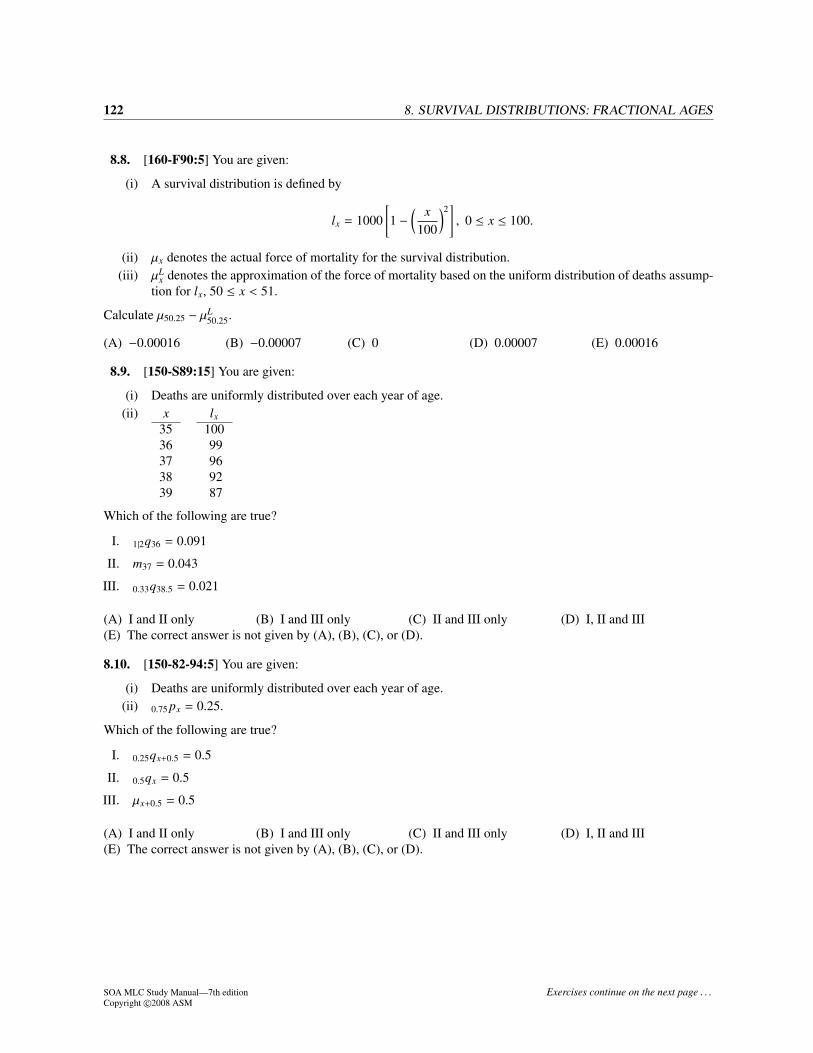
8.8. [160-F90:5] You are given:
(i) A survival distribution is defined by
lx = 1000[1 −
( x100
)2], 0 ≤ x ≤ 100.
(ii) µx denotes the actual force of mortality for the survival distribution.(iii) µL
x denotes the approximation of the force of mortality based on the uniform distribution of deaths assump-tion for lx, 50 ≤ x < 51.
Calculate µ50.25 − µL50.25.
(A) −0.00016 (B) −0.00007 (C) 0 (D) 0.00007 (E) 0.00016
8.9. [150-S89:15] You are given:
(i) Deaths are uniformly distributed over each year of age.(ii) x lx
35 10036 9937 9638 9239 87
Which of the following are true?
I. 1|2q36 = 0.091
II. m37 = 0.043
III. 0.33q38.5 = 0.021
(A) I and II only (B) I and III only (C) II and III only (D) I, II and III(E) The correct answer is not given by (A), (B), (C), or (D).
8.10. [150-82-94:5] You are given:
(i) Deaths are uniformly distributed over each year of age.(ii) 0.75 px = 0.25.
Which of the following are true?
I. 0.25qx+0.5 = 0.5
II. 0.5qx = 0.5
III. µx+0.5 = 0.5
(A) I and II only (B) I and III only (C) II and III only (D) I, II and III(E) The correct answer is not given by (A), (B), (C), or (D).
SOA MLC Study Manual—7th editionCopyright©2008 ASM
Exercises continue on the next page . . .

EXERCISES FOR LESSON 8 123
8.11. [3-S00:12] For a certain mortality table, you are given:
(i) µ(80.5) = 0.0202(ii) µ(81.5) = 0.0408
(iii) µ(82.5) = 0.0619(iv) Deaths are uniformly distributed between integral ages.
Calculate the probability that a person age 80.5 will die within two years.
(A) 0.0782 (B) 0.0785 (C) 0.0790 (D) 0.0796 (E) 0.0800
8.12. You are given:
(i) Deaths are uniformly distributed between integral ages.(ii) qx = 0.1.
(iii) qx+1 = 0.3.
Calculate e̊x+0.7:1 .
8.13. You are given:
(i) Deaths are uniformly distributed between integral ages.(ii) q45 = 0.01.
(iii) q46 = 0.011.
Calculate the variance of the 2-year temporary complete life expectancy on (45).
8.14. You are given:
(i) Deaths are uniformly distributed between integral ages.(ii) 10 px = 0.2.
Calculate e̊x:10 − ex:10 .
8.15. [4-F86:21] You are given:
(i) q60 = 0.020(ii) q61 = 0.022
(iii) Deaths are uniformly distributed over each year of age.
Calculate e̊60:1.5 .
(A) 1.447 (B) 1.457 (C) 1.467 (D) 1.477 (E) 1.487
8.16. [150-F89:21] You are given:
(i) q70 = 0.040(ii) q71 = 0.044
(iii) Deaths are uniformly distributed over each year of age.
Calculate e̊70:1.5 .
(A) 1.435 (B) 1.445 (C) 1.455 (D) 1.465 (E) 1.475
SOA MLC Study Manual—7th editionCopyright©2008 ASM
Exercises continue on the next page . . .

124 8. SURVIVAL DISTRIBUTIONS: FRACTIONAL AGES
8.17. [3-S01:33] For a 4-year college, you are given the following probabilities for dropout from all causes:
q0 = 0.15q1 = 0.10q2 = 0.05q3 = 0.01
Dropouts are uniformly distributed over each year.Compute the temporary 1.5-year complete expected college lifetime of a student entering the second year, e̊1:1.5 .
(A) 1.25 (B) 1.30 (C) 1.35 (D) 1.40 (E) 1.45
8.18. You are given:
(i) Deaths are uniformly distributed between integral ages.(ii) e̊x+0.5:0.5 = 5
12 .
Calculate qx.
8.19. [150-S87:21] You are given:
(i) dx = k for x = 0, 1, 2, . . . , ω − 1(ii) e̊20:20 = 18
(iii) Deaths are uniformly distributed over each year of age.
Calculate 30|10q30.
(A) 0.111 (B) 0.125 (C) 0.143 (D) 0.167 (E) 0.200
8.20. [150-S89:24] You are given:
(i) Deaths are uniformly distributed over each year of age.(ii) µ45.5 = 0.5
Calculate e̊45:1 .
(A) 0.4 (B) 0.5 (C) 0.6 (D) 0.7 (E) 0.8
8.21. [CAS3-S04:10] 4,000 people age (30) each pay an amount, P, into a fund. Immediately after the 1,000th
death, the fund will be dissolved and each of the survivors will be paid $50,000.
• Mortality follows the Illustrative Life Table, using linear interpolation at fractional ages.
• i = 12%
Calculate P.
(A) Less than 515(B) At least 515, but less than 525(C) At least 525, but less than 535(D) At least 535, but less than 545(E) At least 545
SOA MLC Study Manual—7th editionCopyright©2008 ASM
Exercises continue on the next page . . .

EXERCISES FOR LESSON 8 125
8.22. [160-F87:5] Based on given values of lx and lx+1, 1/4 px+1/4 = 49/50 under the assumption of constant forceof mortality.
Calculate 1/4 px+1/4 under the uniform distribution of deaths hypothesis.
(A) 0.9799 (B) 0.9800 (C) 0.9801 (D) 0.9802 (E) 0.9803
8.23. [160-S89:5] A mortality study is conducted for the age interval (x, x + 1].If a constant force of mortality applies over the interval, 0.25qx+0.1 = 0.05.Calculate 0.25qx+0.1 assuming a uniform distribution of deaths applies over the interval.
(A) 0.044 (B) 0.047 (C) 0.050 (D) 0.053 (E) 0.056
8.24. [150-F89:29] You are given that qx = 0.25.Based on the constant force of mortality assumption, the force of mortality is µA
x+s, 0 < s < 1.Based on the uniform distribution of deaths assumption, the force of mortality is µB
x+s, 0 < s < 1.Calculate the smallest s such that µB
x+s ≥ µAx+s.
(A) 0.4523 (B) 0.4758 (C) 0.5001 (D) 0.5242 (E) 0.5477
8.25. [160-S91:4] From a population mortality study, you are given:
(i) Within each age interval, (x + k, x + k + 1], the force of mortality, µx+k, is constant.
(ii) k e−µx+k 1−e−µx+k
µx+k
0 0.98 0.991 0.96 0.98
Calculate e̊x:2 , the expected lifetime in years over (x, x + 2].
(A) 1.92 (B) 1.94 (C) 1.95 (D) 1.96 (E) 1.97
8.26. [150-81-94:50] You are given:
s(x) =(10 − x)2
1000 ≤ x ≤ 10
Instead of using s(x) within each year of age, use the constant force of mortality assumption to calculate the averagenumber of years lived between ages 1 and 2 by those of the survivorship group who die between those ages.
(A) 0.461 (B) 0.480 (C) 0.490 (D) 0.500 (E) 0.508
SOA MLC Study Manual—7th editionCopyright©2008 ASM
Exercises continue on the next page . . .

126 8. SURVIVAL DISTRIBUTIONS: FRACTIONAL AGES
8.27. [3-S01:27] An actuary is modeling the mortality of a group of 1000 people, each age 95, for the next threeyears.
The actuary starts by calculating the expected number of survivors at each integral age by
l95+k = 1000 k p95, k = 1, 2, 3
The actuary subsequently calculates the expected number of survivors at the middle of each year using the assump-tion that deaths are uniformly distributed over each year of age.
This is the result of the actuary’s model:
Age Survivors95 100095.5 80096 60096.5 48097 —97.5 28898 —
The actuary decides to change his assumption for mortality at fractional ages to the constant force assumption.He retains his original assumption for each k p95.
Calculate the revised expected number of survivors at age 97.5
(A) 270 (B) 273 (C) 276 (D) 279 (E) 282
8.28. [160-S87:3] You are analyzing death rates within the age interval [x, x + 1]. You are given that dx > 0.Death rates are calculated according to the following assumptions:
Mortality Rate Assumption
12qU
x Uniform distribution of deaths12qB
x Balducci hypothesis12qC
x Constant force of mortality
Which of the following is correct?
(A) 12qU
x < 12qB
x < 12qC
x
(B) 12qU
x < 12qC
x < 12qB
x
(C) 12qB
x < 12qC
x < 12qU
x
(D) 12qC
x < 12qU
x < 12qB
x
(E) 12qC
x < 12qB
x < 12qU
x
SOA MLC Study Manual—7th editionCopyright©2008 ASM
Exercises continue on the next page . . .

EXERCISES FOR LESSON 8 127
8.29. [150-F86:17] You are given 1000 1/4qx = 2.Rank 1/4qx+3/4 under the Balducci hypothesis, the uniform distribution of deaths (UDD) hypothesis, and the
constant force of mortality hypothesis.
(A) Balducci < constant force < UDD(B) Constant force < Balducci < UDD(C) UDD < constant force < Balducci(D) UDD < Balducci < constant force(E) Balducci < UDD < constant force
8.30. [160-F86:13] You are given that lx = 284 and lx+1 = 236.For some t, 0 < t < 1, the hyperbolic assumption for deaths within a year produces lx+t = 248.For some u, 0 < u < 1, the assumption of uniform deaths within a year produces lx+u = 248.Determine t − u.
(A) −0.079 (B) −0.036 (C) 0.000 (D) 0.036 (E) 0.079
8.31. [160-S88:6] There is an age (x + s) in the interval (x, x + 12 ) such that 13/16−sqx+s has the same value under
both the hyperbolic and uniform assumptions over (x, x + 1].Determine s.
(A) 316 (B) 4
16 (C) 516 (D) 6
16 (E) 716
8.32. [150-S88:25] You are given:
(i) 0.5 pxµx+0.5 = 12/49(ii) Mortality follows the Balducci assumption.
(iii) qx < px
Calculate qx.
(A) 0.25 (B) 0.30 (C) 0.35 (D) 0.40 (E) 0.45
8.33. [160-S89:4] Under the hyperbolic survival assumption for lx+s in the interval (x, x+1], which of the followingare true?
I. 12qx ≥ 1
2qx+1/2
II. s px =px
px+sqx
III. sqx = sµx+s
IV. lx+ 12
= 2lxlx+1lx+lx+1
(A) All but I (B) All but II (C) All but III (D) All but IV (E) All
SOA MLC Study Manual—7th editionCopyright©2008 ASM
Exercises continue on the next page . . .

128 8. SURVIVAL DISTRIBUTIONS: FRACTIONAL AGES
8.34. [150-F88:29] For integral values of x and 0 < s < 1, you are given:
(i) µAx+s is based on the uniform distribution of deaths assumption.
(ii) µBx+s is based on the Balducci distribution of deaths assumption.
Which of the following are true for 0.5 ≤ t < 1?
I. µAx+t = tdx
lx−tdx
II. µBx+t = dx
lx−(1−t)dx
III. µAx+t ≤ µB
x+t
(A) I and II only (B) I and III only (C) II and III only (D) I, II and III(E) The correct answer is not given by (A), (B), (C), or (D).
8.35. [160-S91:3] You are given:
(i) lx = 100,000x2 , for positive integer values of x.
(ii) Under the hyperbolic assumption over (y, y + 1] for some integer y, ly+s = 911, where 0 < s < 1.
Calculate 1−sqy+s under the uniform distribution of deaths assumption.
(A) 0.087 (B) 0.091 (C) 0.093 (D) 0.095 (E) 0.101
8.36. [150-S91:20] You are given:
(i) e̊x:1 = F under the uniform distribution of deaths assumption.(ii) e̊x:1 = G under the Balducci assumption.
(iii) qx = 0.1.
Calculate 1000(F −G).
(A) 0.00 (B) 0.24 (C) 1.00 (D) 1.76 (E) 2.52
8.37. [150-S91:28] You are given that qx = 0.1200.Which of the following are true?
(i) 1/3qx+1/2 = 0.0426 under the uniform distribution of deaths assumption.(ii) 1/3qx = 0.0435 under the Balducci assumption.
(iii) 1/2qx = 0.0619 under the constant force of mortality assumption.
(A) I and II only (B) I and III only (C) II and III only (D) I, II and III(E) The correct answer is not given by (A), (B), (C), or (D).
8.38. [150-81-94:23] You are given:
(i) q60 = 0.3(ii) q61 = 0.4
(iii) f is the probability that (60) will die between ages 60.5 and 61.5 under the uniform distribution of deathsassumption.
(iv) g is the probability that (60) will die between ages 60.5 and 61.5 under the Balducci assumption.
Calculate 10,000(g − f ).
(A) 0 (B) 85 (C) 94 (D) 178 (E) 213
SOA MLC Study Manual—7th editionCopyright©2008 ASM
Exercises continue on the next page . . .

EXERCISES FOR LESSON 8 129
8.39. [3-S01:13] Mr. Ucci has only 3 hairs left on his head and he won’t be growing any more.
(i) The future mortality of each hair follows
k|qx = 0.1(k + 1), k = 0, 1, 2, 3 and x is Mr. Ucci’s age
(ii) Hair loss follows the hyperbolic assumption at fractional ages.(iii) The future lifetimes of the 3 hairs are independent.
Calculate the probability that Mr. Ucci is bald (has no hair left) at age x + 2.5.
(A) 0.090 (B) 0.097 (C) 0.104 (D) 0.111 (E) 0.118
8.40. [SOA3-F03:16] For a space probe to Mars:
(i) The probe has three radios, whose future lifetimes are independent, each with mortality following
k|q0 = 0.1(k + 1), k = 0, 1, 2, 3
where time 0 is the moment the probe lands on Mars.(ii) The failure time of each radio follows the hyperbolic assumption within each year.
(iii) The probe will transmit until all three radios have failed.
Calculate the probability that the probe is no longer transmitting 2.25 years after landing on Mars.
(A) 0.053 (B) 0.059 (C) 0.063 (D) 0.067 (E) 0.069
8.41. [SOA3-F03:36] Consider the 1-year temporary complete life expectancy of (90), i.e. e̊90:1 , as based on theIllustrative Life Table. Let C, H, and U be its values under the constant force, the hyperbolic, and the uniformdistribution assumptions respectively.
Which of the following is true?
(A) C > H > U(B) C > U > H(C) U > C > H(D) U > H > C(E) H = C = U
8.42. [160-S91:5] With respect to the interval (x, x + 1], you are given:
(i) px = 0.5(ii) mH
x denotes the central death rate under the hyperbolic assumption.(iii) mE
x denotes the central death rate under the exponential assumption.
Calculate mHx − mE
x .
(A) −0.028 (B) −0.026 (C) 0.000 (D) 0.026 (E) 0.028Additional released exam questions: CAS3-S05:31, CAS3-F05:13, CAS3-S06:13, CAS3-F06:13,SOA M-F06:16, CAS3-S07:24, CAS3L-S08:16
SOA MLC Study Manual—7th editionCopyright©2008 ASM
130 8. SURVIVAL DISTRIBUTIONS: FRACTIONAL AGES
Solutions
8.1. 1/2 pxµx+1/2 is the density function, or qx. 3/4 px = 1 − 34 qx. So the sum is 1 − 1
4 qx, or 1/4 px . (E)
8.2. Using equation (8.2),
331
= 0.25qx+0.75 =0.25qx
1 − 0.75qx
331− 2.25
31qx = 0.25qx
331
=1031
qx
qx = 0.3
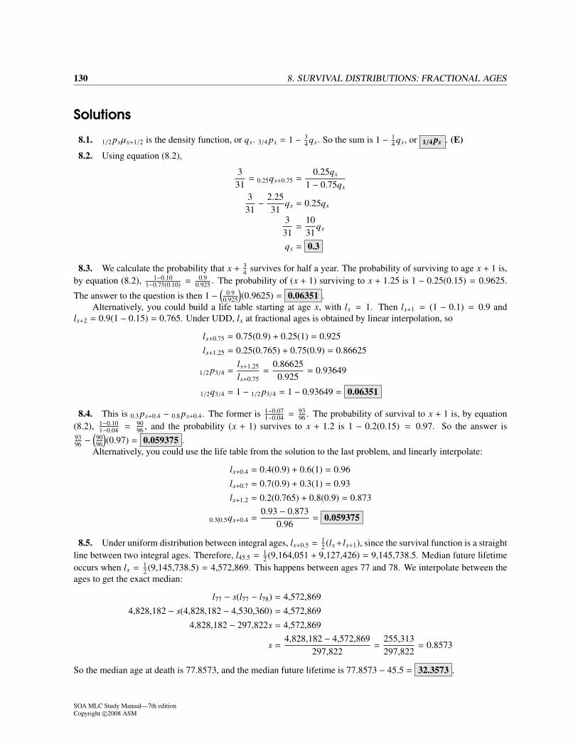
8.3. We calculate the probability that x + 34 survives for half a year. The probability of surviving to age x + 1 is,
by equation (8.2), 1−0.101−0.75(0.10) = 0.9
0.925 . The probability of (x + 1) surviving to x + 1.25 is 1 − 0.25(0.15) = 0.9625.
The answer to the question is then 1 −(
0.90.925
)(0.9625) = 0.06351 .
Alternatively, you could build a life table starting at age x, with lx = 1. Then lx+1 = (1 − 0.1) = 0.9 andlx+2 = 0.9(1 − 0.15) = 0.765. Under UDD, lx at fractional ages is obtained by linear interpolation, so
lx+0.75 = 0.75(0.9) + 0.25(1) = 0.925lx+1.25 = 0.25(0.765) + 0.75(0.9) = 0.86625
1/2 p3/4 =lx+1.25
lx+0.75=
0.866250.925
= 0.93649
1/2q3/4 = 1 − 1/2 p3/4 = 1 − 0.93649 = 0.06351
8.4. This is 0.3 px+0.4 − 0.8 px+0.4. The former is 1−0.071−0.04 = 93
96 . The probability of survival to x + 1 is, by equation(8.2), 1−0.10
1−0.04 = 9096 , and the probability (x + 1) survives to x + 1.2 is 1 − 0.2(0.15) = 0.97. So the answer is
9396 −
(9096
)(0.97) = 0.059375 .
Alternatively, you could use the life table from the solution to the last problem, and linearly interpolate:
lx+0.4 = 0.4(0.9) + 0.6(1) = 0.96lx+0.7 = 0.7(0.9) + 0.3(1) = 0.93lx+1.2 = 0.2(0.765) + 0.8(0.9) = 0.873
0.3|0.5qx+0.4 =0.93 − 0.873
0.96= 0.059375
8.5. Under uniform distribution between integral ages, lx+0.5 = 12 (lx +lx+1), since the survival function is a straight
line between two integral ages. Therefore, l45.5 = 12 (9,164,051 + 9,127,426) = 9,145,738.5. Median future lifetime
occurs when lx = 12 (9,145,738.5) = 4,572,869. This happens between ages 77 and 78. We interpolate between the
ages to get the exact median:
l77 − s(l77 − l78) = 4,572,8694,828,182 − s(4,828,182 − 4,530,360) = 4,572,869
4,828,182 − 297,822s = 4,572,869
s =4,828,182 − 4,572,869
297,822=
255,313297,822
= 0.8573
So the median age at death is 77.8573, and the median future lifetime is 77.8573 − 45.5 = 32.3573 .
SOA MLC Study Manual—7th editionCopyright©2008 ASM

EXERCISE SOLUTIONS FOR LESSON 8 131
8.6. First we use equation (8.4) to get qx.
0.04 = µx+0.75 =qx
1 − 0.75qx
0.04 − 0.03qx = qx
qx =4
103
Then from equation (8.5),
mx =
4103
1 − 2103
=4
101
8.7. We use the fact that for each age, Lx = 12 (lx + lx+1), so 3L52 = 1
2 (l52 + 2l53 + 2l54 + l55), and we have
3m52 =3d52
12 (l52 + 2l53 + 2l54 + l55)
Dividing numerator and denominator by l52
=23q52
1 + 2p52 + 22 p52 + 3 p52
=2[1 − (0.90)(0.89)(0.87)]
1 + 2(0.90) + 2(0.90)(0.89) + (0.90)(0.89)(0.87)
=0.606265.09887
= 0.11890
8.8. x p0 = lxl0
= 1 −(
x100
)2. The force of mortality is calculated as the derivative of ln x p0:
µx = −d ln x p0
dx=
2(
x100
)(1
100
)
1 −(
x100
)2 =2x
1002 − x2
and µ50.25 = 100.51002−50.252 = 0.0134449.
p50 = 1−0.512
1−0.502 = 0.986533 and q50 = 1 − 0.986533 = 0.013467, so under UDD,
µL50.25 =
q50
1 − 0.25q50=
0.0134671 − 0.25(0.013467)
= 0.013512.
The difference is 0.013445 − 0.013512 = −0.000067 . (B)
8.9. 1|2q36 = 2d37l36
= 96−8799 = 0.09091, so I is true. This statement does not require uniform distribution of deaths.
By equation (8.5), m37 =2d37
l37+l38=
2(4)96+92 = 0.042553, so II is true.
0.33q38.5 is 0.33d38.5l38.5
, which is (0.33)(5)89.5 = 0.018436, so III is false. I can’t figure out what mistake you’d have to
make to get 0.021. (A)8.10. First calculate qx.
1 − 0.75qx = 0.25qx = 1
Then by equation (8.2), 0.25qx+0.5 = 0.251−0.5 = 0.5, making I true.
By equation (8.1), 0.5qx = 0.5qx = 0.5, making II true.By equation (8.4), µx+0.5 = 1
1−0.5 = 2, making III false. (A)
SOA MLC Study Manual—7th editionCopyright©2008 ASM

132 8. SURVIVAL DISTRIBUTIONS: FRACTIONAL AGES
8.11. We use equation (8.4) to back out qx for each age.
µx+0.5 =qx
1 − 0.5qx⇒ qx =
µx+0.5
1 + 0.5µx+0.5
q80 =0.02021.0101
= 0.02
q81 =0.04081.0204
= 0.04
q82 =0.06191.03095
= 0.06
Then by equation (8.2), 0.5 p80.5 = 0.980.99 . p81 = 0.96 and 0.5 p82 = 1 − 0.5(0.6) = 0.97. Therefore
2q80.5 = 1 −(0.980.99
)(0.96)(0.97) = 0.0782 (A)
8.12. To do this algebraically, we split the group into those who die within 0.3 years, those who die between 0.3and 1 years, and those who survive one year. Under UDD, those who die will die at the midpoint of the interval(assuming the interval doesn’t cross an integral age), so we have
Group Survival Probability AverageGroup time of group survival time
I (0, 0.3] 1 − 0.3 px+0.7 0.15II (0.3, 1] 0.3 px+0.7 − 1 px+0.7 0.65III (1,∞) 1 px+0.7 1
We calculate the required probabilities.
0.3 px+0.7 =0.9
0.93= 0.967742
1 px+0.7 =0.9
0.93[1 − 0.7(0.3)] = 0.764516
1 − 0.3 px+0.7 = 1 − 0.967742 = 0.032258
0.3 px+0.7 − 1 px+0.7 = 0.967742 − 0.764516 = 0.203226
e̊x+0.7:1 = 0.032258(0.15) + 0.203226(0.65) + 0.764516(1) = 0.901452
Alternatively, we can use trapezoids. We already know from the above solution that the heights of the firsttrapezoid are 1 1 and 0.967742, and the heights of the second trapezoid are 0.967742 and 0.764516. So the sum ofthe area of the two trapezoids is
e̊x+0.7:1 = (0.3)(0.5)(1 + 0.967742) + (0.7)(0.5)(0.967742 + 0.764516)
= 0.295161 + 0.606290 = 0.901451
8.13. For the expected value, we’ll use the recursive formula. (The trapezoidal rule could also be used.)
e̊45:2 = e̊45:1 + p45e̊46:1
= (1 − 0.005) + 0.99(1 − 0.0055)= 1.979555
We’ll use the formula in terms of t px for the second moment.
E[T 2] = 2∫ 2
0tt pxdt
SOA MLC Study Manual—7th editionCopyright©2008 ASM

EXERCISE SOLUTIONS FOR LESSON 8 133
= 2[∫ 1
0t(1 − 0.01t)dt +
∫ 2
1t(0.99)[1 − 0.011(t − 1)]dt
]
= 2{
12− 0.01
(13
)+ 0.99
[(1.011)(22 − 12)
2− 0.011
(23 − 13
3
)]}
= 2(0.49667 + 1.475925) = 3.94518
So the variance is 3.94518 − 1.9795552 = 0.02654 .8.14. As discussed on page 8.7, by equation (8.7), the difference is
12 10qx =
12
(1 − 0.2) = 0.4
8.15. Those who die in the first year survive 12 year on the average and those who die in the first half of the second
year survive 1.25 years on the average, so we have
p60 = 0.98
1.5 p60 = 0.98[1 − 0.5(0.022)
]= 0.96922
e̊60:1.5 = 0.5(0.02) + 1.25(0.98 − 0.96922) + 1.5(0.96922) = 1.477305 (D)
Alternatively, we use the trapezoidal method.
e̊60:1.5 =12
(1 + 0.98) +
(12
)(12
){0.98 + 0.98
[1 − 0.5(0.022)
]}
= 1.477305 (D)
8.16. p70 = 1 − 0.040 = 0.96, 2 p70 = (0.96)(0.956) = 0.91776, and by linear interpolation, 1.5 p70 = 0.5(0.96 +
0.91776) = 0.93888. Those who die in the first year survive 0.5 years on the average and those who die in the firsthalf of the second year survive 1.25 years on the average. So
e̊70:1.5 = 0.5(0.04) + 1.25(0.96 − 0.93888) + 1.5(0.93888) = 1.45472 (C)
Alternatively, we can use the trapezoidal method. The first year’s trapezoid has heights 1 and 0.96 and thesecond year’s trapezoid has heights 0.96 and 0.93888, so
e̊70:1.5 = 0.5(1 + 0.96) + 0.5(0.5)(0.96 + 0.93888) = 1.45472 (C)
8.17. First we calculate t p1 for t = 1, 2.
p1 = 1 − q1 = 0.90
2 p1 = (1 − q1)(1 − q2) = (0.90)(0.95) = 0.855
By linear interpolation, 1.5 p1 = (0.5)(0.9 + 0.855) = 0.8775.The algebraic method splits the students into 3 groups: first year dropouts, second year (through time 1.5)
dropouts, and survivors. In each dropout group survival on the average is to the midpoint (0.5 years for the firstgroup, 1.25 years for the second group) and survivors survive 1.5 years. Therefore
e̊1:1.5 = 0.10(0.5) + (0.90 − 0.8775)(1.25) + 0.8775(1.5) = 1.394375 (D)
SOA MLC Study Manual—7th editionCopyright©2008 ASM

134 8. SURVIVAL DISTRIBUTIONS: FRACTIONAL AGES
1 2 2.5 3
1
x
t p1
(2, 0.9) (2.5,0.8775)
Alternatively, we could sum the two trapezoids making up the shaded areaat the right.
e̊1:1.5 = (1)(0.5)(1 + 0.9) + (0.5)(0.5)(0.90 + 0.8775)
= 0.95 + 0.444375 = 1.394375 (D)
8.18. Those who die survive 0.25 years on the average and survivors survive 0.5 years, so we have
0.25 0.5qx+0.5 + 0.5 0.5 px+0.5 = 512
0.25(
0.5qx
1 − 0.5qx
)+ 0.5
(1 − qx
1 − 0.5qx
)= 5
12
0.125qx + 0.5 − 0.5qx = 512 − 5
24 qx
12− 5
12=
[524
+12− 1
8
]qx
112
=qx
6
qx = 12
512
0.5 1x
t px+0.5
1
0.5 px+0.5
Alternatively, complete life expectancy is the area of the trapezoidshown on the right, so
512
= 0.5(0.5)(1 + 0.5 px+0.5)
Then 0.5 px+0.5 = 23 , from which it follows
23
=1 − qx
1 − 12 qx
qx = 12
8.19. Since dx is constant for all x and deaths are uniformly distributed within each year of age, mortality followsde Moivre’s law. We back out ω. Complete life expectancy is the area of the trapezoid shown below.
18
20 40x
lx
1ω − 40ω − 20
e̊20:20 = 18 = (20)(0.5)(1 +
ω − 40ω − 20
)
0.8 =ω − 40ω − 20
0.8ω − 16 = ω − 400.2ω = 24
ω = 120
Alternatively, we split the population into 2 groups. Those who die within 20 years survive 10 years on theaverage and the others survive 20 years, so
10 20q20 + 20 20 p20 = 18
SOA MLC Study Manual—7th editionCopyright©2008 ASM

EXERCISE SOLUTIONS FOR LESSON 8 135
10(
20ω − 20
)+ 20
(ω − 40ω − 20
)= 18
200 + 20ω − 800 = 18ω − 3602ω = 240ω = 120
Once we have ω, we compute 30|10q30 = 10ω−30 = 10
90 = 0.1111 . (A)8.20. We use equation (8.4) to obtain
0.5 =qx
1 − 0.5qx
qx = 0.4
Then e̊45:1 = 0.5[1 + (1 − 0.4)] = 0.8 . (E)8.21. According to the Illustrative Life Table, l30 = 9,501,381, so we are looking for the age x such that lx =
0.75(9,501,381) = 7,126,0.36. This is between 67 and 68. Using linear interpolation, since l67 = 7,201,635 andl68 = 7,018,432, we have
x = 67 +7,201,635 − 7,126,0367,201,635 − 7,018,432
= 67.4127
This is 37.4127 years into the future. 34 of the people collect 50,000. We need 50,000
(34
)(1
1.1237.4127
)= 540.32 per
person. (D)8.22. Under constant force of mortality, s px+t = ps
x, so px = 1/4 p4x+1/4 = 0.984 = 0.922368 and qx = 1−0.922368 =
0.077632. Under uniform distribution of deaths,
1/4 px+1/4 = 1 − (1/4)qx
1 − (1/4)qx
= 1 − (1/4)(0.077632)1 − (1/4)(0.077632)
= 1 − 0.019792 = 0.980208 (D)
8.23. Under constant force, s px+t = psx, so px = 0.954 = 0.814506, qx = 1 − 0.814506 = 0.185494. Then under a
uniform assumption,
0.25qx+0.1 =0.25qx
1 − 0.1qx=
(0.25)(0.185494)1 − 0.1(0.185494)
= 0.047250 (B)
8.24. For constant force, µA is a constant, equal to − ln px = − ln 0.75 = 0.2877. Then
µBx+s =
qx
1 − sqx= 0.2877
0.251 − 0.25s
= 0.2877
0.2877 − 0.25(0.2877)s = 0.25
s =0.2877 − 0.25(0.25)(0.2877)
= 0.5242 (D)
SOA MLC Study Manual—7th editionCopyright©2008 ASM

136 8. SURVIVAL DISTRIBUTIONS: FRACTIONAL AGES
8.25. We integrate t px from 0 to 2. Between 0 and 1, t px = e−tµx .∫ 1
0e−tµx dt =
1 − eµx
µx= 0.99
Between 1 and 2, t px = px t−1 px+1 = 0.98e−(t−1)µx+1 .∫ 2
1e−(t−1)µx+1 =
1 − eµx+1
µx+1= 0.98
So the answer is 0.99 + 0.98(0.98) = 1.9504 . (C)8.26. We calculate the temporary expectation of life for one-year, e̊1:1 , subtract p1 for the amount lived by thosewho survive, then divide by q1. p1 and q1 don’t use constant force of mortality assumption.
p1 =s(2)s(1)
=(10 − 2)2
(10 − 1)2 =6481
q1 = 1 − p1 =1781
For constant force, t p1 = e−tµ for t < 1. Since p1 = e−µ, µ = − ln 6481 = 0.235566. Then
e̊1:1 =
∫ 1
0t p1dt
=
∫ 1
0e−tµdt
=1 − e−µ
µ
=q1
µ=
17/810.235566
= 0.890946
Thena(1) =
0.890946 − (64/81)17/81
= 0.480388 (B)
8.27. Under uniform distribution, the numbers of deaths in each half of the year are equal, so if 120 deathsoccurred in the first half of x = 96, then 120 occurred in the second half, and l97 = 480 − 120 = 360. Then if0.5q97 = 360−288
360 = 0.2, then q97 = 2 0.5q97 = 0.4, so p97 = 0.6. Under constant force, 1/2 p97 = p0.597 =
√0.6. The
answer is 360√
0.6 = 278.8548 . (D)8.28. The Balducci hypothesis speeds up deaths the most and the uniform hypothesis speeds them up the least, sothe answer is (B).8.29. In general, Balducci speeds up the deaths the most and UDD the least. When looking at deaths in the lastquarter of the year, this means Balducci will have the least and UDD the most, or (A).
They gave you 1/4qx to help make it more concrete. Under constant force of mortality, this equals 1/4qx+3/4,while under Balducci 1/4qx+s is a decreasing function of s and under UDD 1/4qx+s is an increasing function of s.8.30. For the hyperbolic assumption,
lx+t =lxlx+1
lx+1 + t(lx − lx+1)
248 =(236)(284)236 + 48t
SOA MLC Study Manual—7th editionCopyright©2008 ASM

EXERCISE SOLUTIONS FOR LESSON 8 137
236 + 48t =(236)(284)
248= 270.2581
t =270.2581 − 236
48= 0.71371
For the uniform assumption, 248 = 284 + u(236 − 284) = 284 − 48u which yields u = 0.75. t − u =
0.71371 − 0.75 = −0.03629 . (B)8.31. For the uniform hypothesis,
13/16−sqx+s =
(1316 − s
)qx
1 − sqx.
For the hyperbolic hypothesis,
13/16−s px+s =13/16 px
s px
=1 − (1 − s)qx
1 − [1 − (13/16)]qx
=1 − (1 − s)qx
1 − (3/16)qx
13/16−sqx+s =
(1316 − s
)qx
1 − (3/16)qx
The numerators are equal. Equating the denominators, we get s = 316 . (A)
8.32.
t pxµx+t =pxqx
(px + tqx)2
1249
=(1 − qx)(qx)
[1 − (1/2)qx]2
49qx(1 − qx) = 12(1 − 1
2 qx
)2
49qx − 49q2x = 12 − 12qx + 3q2
x
52q2x − 61qx + 12 = 0
qx =61 ±
√612 − 4(52)(12)
104
Since qx < px, we choose the lower solution, 61−35104 = 0.25 . (A)
8.33. I is true because mortality drops over the year under the hyperbolic assumption. The other formulas arecorrect. (E)8.34. I is incorrect. Dividing numerator and denominator by lx, we have tqx
1−tqx, and there should not be a t in the
numerator.II is correct. Dividing the numerator and denominator by lx we have the formula qx
1−(1−t)qx.
III is the only choice requiring t ≥ 0.5. It is false since µx+t is an increasing function for t under UDD anddecreasing under Balducci. Alternatively, compare the corrected version of I to II; the denominator of I is less thanor (at t = 0.5, or if qx = 0) equal to the denominator of II when t ≥ 0.5. (E)
SOA MLC Study Manual—7th editionCopyright©2008 ASM

138 8. SURVIVAL DISTRIBUTIONS: FRACTIONAL AGES
8.35. First we determine y.
100,000x2 = 911
x =
√100,000
911= 10.477
so y must be 10 so that l10 > 911 and l11 ≤ 911. Then p10 = 102
112 = 0.826446 and q10 = 1 − 0.826446 = 0.173554.We solve for s.
0.911 =p10
p10 + sq10=
0.8264460.826446 + 0.173554s
0.173554s =0.826446
0.911− 0.826446 = 0.080740
s =0.0807400.173554
= 0.465214
Under uniform distribution of deaths,
1−0.465214q10.465214 =(1 − 0.465214)(0.173554)1 − (0.465214)(0.173554)
= 0.100966 (E)
8.36. The best approach is to use e̊x:1 =∫ 1
0 t px dt. Under UDD, the integral is the area of a trapezoid with heights1 and 1 − qx = 0.9 and width 1; the area is F = 0.95. Under Balducci,
t px =px
px + tqx=
0.90.9 + 0.1t
=9
9 + t
G =
∫ 1
0t px dt =
∫ 1
0
9dt9 + t
= 9(ln 10 − ln 9) = 0.948245
1000(F −G) = 1000(0.95 − 0.948245) = 1.755 (D)
8.37. I: 1/3qx+1/2 =
13 qx
1 − 12 qx
=0.040.94
= 0.042553. 3
II: 1/3qx =13qx
1 − 23 qx
=0.040.92
= 0.043478. 3
III: 1/2qx = 1 − p1/2x = 1 − 0.881/2 = 0.061917. 3
(D)8.38. We’ll calculate 1/2 p60 and 3/2 p60. The former minus the latter is the probability of death between ages 60.5and 61.5.
Under UDD, half the deaths occur in the first half of the year and half in the second half, so the probability ofsurviving half a year is 1− 0.5(0.3) = 0.85 and the probability of surviving 1 1
2 years is 0.7[1− 0.5(0.4)] = 0.56. Thedifference is 0.85 − 0.56 = 0.29.
Under Balducci, we have
1/2qx =
12 qx
1 − 12 qx
so 1/2q60 = 0.150.85 and 1/2q61 = 0.2
0.8 . Then 1/2 p60 = 0.70.85 = 0.823529 and 3/2 p60 = (0.7) 0.6
0.8 = 0.525. The difference is0.823529 − 0.525 = 0.298529. So the answer is 10,000(0.298529 − 0.29) = 85.29 . (B)
SOA MLC Study Manual—7th editionCopyright©2008 ASM
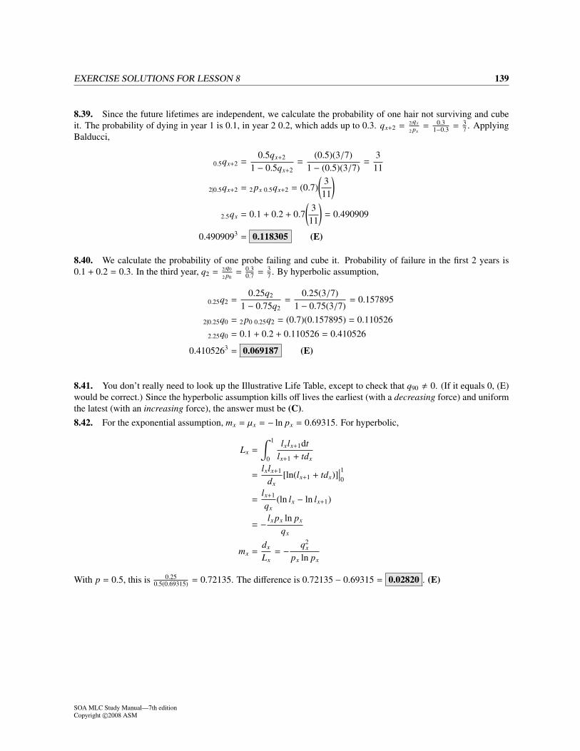
EXERCISE SOLUTIONS FOR LESSON 8 139
8.39. Since the future lifetimes are independent, we calculate the probability of one hair not surviving and cubeit. The probability of dying in year 1 is 0.1, in year 2 0.2, which adds up to 0.3. qx+2 = 2|qx
2 px= 0.3
1−0.3 = 37 . Applying
Balducci,
0.5qx+2 =0.5qx+2
1 − 0.5qx+2=
(0.5)(3/7)1 − (0.5)(3/7)
=3
11
2|0.5qx+2 = 2 px 0.5qx+2 = (0.7)(
311
)
2.5qx = 0.1 + 0.2 + 0.7(
311
)= 0.490909
0.4909093 = 0.118305 (E)
8.40. We calculate the probability of one probe failing and cube it. Probability of failure in the first 2 years is0.1 + 0.2 = 0.3. In the third year, q2 = 2|q0
2 p0= 0.3
0.7 = 37 . By hyperbolic assumption,
0.25q2 =0.25q2
1 − 0.75q2=
0.25(3/7)1 − 0.75(3/7)
= 0.157895
2|0.25q0 = 2 p0 0.25q2 = (0.7)(0.157895) = 0.110526
2.25q0 = 0.1 + 0.2 + 0.110526 = 0.410526
0.4105263 = 0.069187 (E)
8.41. You don’t really need to look up the Illustrative Life Table, except to check that q90 , 0. (If it equals 0, (E)would be correct.) Since the hyperbolic assumption kills off lives the earliest (with a decreasing force) and uniformthe latest (with an increasing force), the answer must be (C).8.42. For the exponential assumption, mx = µx = − ln px = 0.69315. For hyperbolic,
Lx =
∫ 1
0
lxlx+1dtlx+1 + tdx
=lxlx+1
dx[ln(lx+1 + tdx)]
∣∣∣10
=lx+1
qx(ln lx − ln lx+1)
= − lx px ln px
qx
mx =dx
Lx= − q2
x
px ln px
With p = 0.5, this is 0.250.5(0.69315) = 0.72135. The difference is 0.72135 − 0.69315 = 0.02820 . (E)
SOA MLC Study Manual—7th editionCopyright©2008 ASM
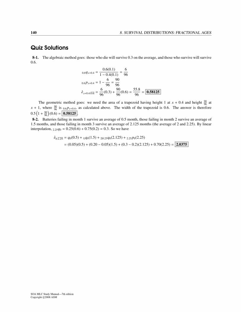
140 8. SURVIVAL DISTRIBUTIONS: FRACTIONAL AGES
Quiz Solutions
8-1. The algebraic method goes: those who die will survive 0.3 on the average, and those who survive will survive0.6.
0.6qx+0.4 =0.6(0.1)
1 − 0.4(0.1)=
696
0.6 px+0.4 = 1 − 696
=9096
e̊x+0.4:0.6 =696
(0.3) +9096
(0.6) =55.896
= 0.58125
The geometric method goes: we need the area of a trapezoid having height 1 at x + 0.4 and height 9096 at
x + 1, where 9096 is 0.6 px+0.4, as calculated above. The width of the trapezoid is 0.6. The answer is therefore
0.5(1 + 90
96
)(0.6) = 0.58125 .
8-2. Batteries failing in month 1 survive an average of 0.5 month, those failing in month 2 survive an average of1.5 months, and those failing in month 3 survive an average of 2.125 months (the average of 2 and 2.25). By linearinterpolation, 2.25q0 = 0.25(0.6) + 0.75(0.2) = 0.3. So we have
e̊0:2.25 = q0(0.5) + 1|q0(1.5) + 2|0.25q0(2.125) + 2.25 p0(2.25)
= (0.05)(0.5) + (0.20 − 0.05)(1.5) + (0.3 − 0.2)(2.125) + 0.70(2.25) = 2.0375
SOA MLC Study Manual—7th editionCopyright©2008 ASM