Embed Size (px)
Citation preview

3GPP
3GPP TR 25.863 V10.0.0 (2010-07)Technical Specification
3rd Generation Partnership Project;Technical Specification Group Radio Access Network;
Universal Terrestrial Radio Access (UTRA); Uplink transmit diversity for High Speed Packet Access
(HSPA) (Release 10)
The present document has been developed within the 3rd Generation Partnership Project (3GPP TM) and may be further elaborated for the purposes of 3GPP. The present document has not been subject to any approval process by the 3GPP Organizational Partners and shall not be implemented. This Specification is provided for future development work within 3GPP only. The Organizational Partners accept no liability for any use of this Specification. Specifications and reports for implementation of the 3GPP TM system should be obtained via the 3GPP Organizational Partners' Publications Offices.

2
3GPP
Error! No text of specified
3GPP TR 25.863 V10.0.0 (2010-07)
Keywords UMTS, Radio
3GPP
Postal address
3GPP support office address 650 Route des Lucioles - Sophia Antipolis
Valbonne - FRANCE Tel.: +33 4 92 94 42 00 Fax: +33 4 93 65 47 16
Internet http://www.3gpp.org
Copyright Notification
No part may be reproduced except as authorized by written permission. The copyright and the foregoing restriction extend to reproduction in all media.
© 2010, 3GPP Organizational Partners (ARIB, ATIS, CCSA, ETSI, TTA, TTC).
All rights reserved. UMTS™ is a Trade Mark of ETSI registered for the benefit of its members 3GPP™ is a Trade Mark of ETSI registered for the benefit of its Members and of the 3GPP Organizational Partners LTE™ is a Trade Mark of ETSI currently being registered for the benefit of its Members and of the 3GPP Organizational Partners GSM® and the GSM logo are registered and owned by the GSM Association

3
3GPP
Error! No text of specified
3GPP TR 25.863 V10.0.0 (2010-07)
Contents Foreword ...................................................................................................................................................... 7 1 Scope .................................................................................................................................................. 8 2 References .......................................................................................................................................... 8 3 Definitions, symbols and abbreviations ............................................................................................. 13 3.1 Definitions ....................................................................................................................................................... 13 3.2 Symbols ........................................................................................................................................................... 13 3.3 Abbreviations ................................................................................................................................................... 13 4 Description of Uplink Transmit Diversity Algorithms ....................................................................... 13 4.1 Theoretical Analysis of Uplink Transmit Diversity ......................................................................................... 13 4.1.1 No Transmit Diversity ................................................................................................................................ 13 4.1.2 Switched Antenna Transmit Diversity ....................................................................................................... 14 4.1.3 Beam-forming Transmit Diversity ............................................................................................................. 14 4.2 Genie Algorithms ............................................................................................................................................. 15 4.2.1 Switched Antenna Transmit Diversity ....................................................................................................... 15 4.2.2 Beamforming Transmit Diversity .............................................................................................................. 16 4.3 Practical Algorithms ........................................................................................................................................ 17 4.3.1 Switched Antenna Transmit Diversity ....................................................................................................... 17 4.3.1.1 Switched Antenna Transmit Diversity - Suboptimal Algorithm .......................................................... 17 4.3.2 Beamforming Transmit Diversity .............................................................................................................. 18 5 Link and System Evaluation Methodology ........................................................................................ 20 5.1 Link Simulation Assumptions.......................................................................................................................... 20 5.2 Link Performance Evaluation Metrics ............................................................................................................. 22 5.3 System Simulation Assumptions ..................................................................................................................... 22 5.3.1 Modelling of Antenna Imbalance ............................................................................................................... 22 5.3.2 System Simulation Parameters ................................................................................................................... 35 5.3.3 Modeling of NodeB Receiver Loss in System Simulations ....................................................................... 36 5.3.3.1 On the need to model to NodeB Receiver Loss in System Simulations due to Switched Antenna
Transmit Diversity ................................................................................................................................ 36 5.4 System Performance Evaluation Metrics ......................................................................................................... 39 6 Link Evaluation Results .................................................................................................................... 40 6.1 Switched Antenna Transmit Diversity ............................................................................................................. 40 6.1.1 Genie Algorithms ....................................................................................................................................... 40 6.1.2 Practical Algorithms ................................................................................................................................... 44 6.1.3 Impact of Realistic E-DPCCH Decoding on Switched Antenna Transmit Diversity ................................. 50 6.1.4 HS-DPCCH Performance in Soft Handover with Switched Antenna Transmit Diversity ......................... 52 6.1.4.1 Notation ................................................................................................................................................ 52 6.1.4.2 HS-DPCCH Performance ..................................................................................................................... 53 6.1.5 Sensitivity with respect to the BLER operating point ................................................................................ 53 6.2 Beamforming Transmit Diversity .................................................................................................................... 55 6.2.1 Genie Algorithms ....................................................................................................................................... 55 6.2.2 Practical Algorithms ................................................................................................................................... 58 6.2.2.1 Results for a Practical Node-B .............................................................................................................................. 68 6.2.3 HS-DPCCH Performance in Soft Handover with Beamforming Transmit Diversity ................................ 69 6.2.3.1 Notation ................................................................................................................................................ 69 6.2.3.2 HS-DPCCH Performance ..................................................................................................................... 71 6.3 Uplink Transmit Diversity Link Level Simulations with Discontinuous Transmission .................................. 72 6.3.1 Discontinuous transmission description ..................................................................................................... 72 6.3.2 Link level simulation results ...................................................................................................................... 72 6.4 Uplink Transmit Diversity Link Level Simulations with Soft Handover ........................................................ 73

4
3GPP
Error! No text of specified
3GPP TR 25.863 V10.0.0 (2010-07)
6.4.1 Soft Handover Simulations Description ..................................................................................................... 73 6.4.2 Link Level Simulations Results ................................................................................................................. 73 6.5 Uplink Transmit Diversity Link Level Simulations with Incorrect TPC command delay ............................... 73 6.6 Uplink Transmit Diversity Link Level Simulations with Multipath Propagation ............................................ 74 6.7 Conclusion on Link Evaluation Results ........................................................................................................... 74 6.7.1 Switched Antenna Transmit Diversity ....................................................................................................... 74 6.7.2 Beamforming Transmit Diversity .............................................................................................................. 75 7 System Evaluation Results ................................................................................................................ 76 7.1 Switched Antenna Transmit Diversity ............................................................................................................. 76 7.1.1 Full Buffer Traffic ...................................................................................................................................... 76 7.1.1.1 Results for inter-site distance 1km ....................................................................................................... 76 7.1.1.1.1 Results for 0 dB long-term antenna imbalance and 2D antennas .................................................... 76 7.1.1.1.2 Results for 0 dB long-term antenna imbalance and 3D antenna ..................................................... 82 7.1.1.1.3 Results for -4 dB long-term antenna imbalance and 2D antennas .................................................. 85 7.1.1.1.4 Results for -4 dB long-term antenna imbalance and 3D antennas .................................................. 88 7.1.1.1.5 Results for 0 dB long-term antenna imbalance and 2D antennas with 50 % penetration of SATD
terminals.......................................................................................................................................... 90 7.1.1.1.6 Results for 0 dB long-term antenna imbalance and 2D antennas with 25 % penetration of SATD
terminals and 1 000 m ISD ............................................................................................................. 93 7.1.1.1.6.3 Results for non TX-diversity users ....................................................................................................... 95 7.1.1.1.7 Results for 0 dB long-term antenna imbalance and 2D antennas with 75 % penetration of SATD
terminals and 1 000 m ISD ............................................................................................................. 97 7.1.1.2 Results for inter-site distance 2.8 km ................................................................................................. 102 7.1.1.2.1 Results for 0 dB long-term antenna imbalance and 2D antennas .................................................. 102 7.1.1.2.2 Results for -4 dB long-term antenna imbalance and 2D antennas ................................................ 105 7.1.1.2.3 Results for ISD 2.8 km with 50 % penetration of SATD terminals .............................................. 106 7.1.1.2.4 Results for 0 dB long-term antenna imbalance and 2D antennas with 25 % penetration of SATD
terminals and 2 800 m ISD ........................................................................................................... 109 7.1.1.2.5 Results for 0 dB long-term antenna imbalance and 2D antennas with 75 % penetration of SATD
terminals and 2 800 m ISD ........................................................................................................... 113 7.1.1.3 Sensitivity to BLER target .................................................................................................................. 117 7.1.1.4 System performance evaluation for suboptimal SATD algorithms .................................................... 118 7.1.2 Bursty Traffic ........................................................................................................................................... 120 7.1.2.1 Results for inter-site distance 1 km .................................................................................................... 120 7.1.2.1.1 Results for 0 dB long-term antenna imbalance and 2D antennas .................................................. 120 7.2 Beam-forming Transmit Diversity ................................................................................................................. 129 7.2.1 Full Buffer Traffic .................................................................................................................................... 129 7.2.1.1 Results for inter-site distance 1km ..................................................................................................... 129 7.2.1.1.1 Results for 0 dB long-term antenna imbalance and 2D antennas .................................................. 129 7.2.1.1.2 Results for 0 dB long-term antenna imbalance and 3D antennas .................................................. 138 7.2.1.1.3 Results for -4 dB long-term antenna imbalance and 2D antennas ................................................ 141 7.2.1.1.4 Results for -4 dB long-term antenna imbalance and 3D antennas ................................................ 143 7.2.1.1.5 Results for 0 dB long-term antenna imbalance and 2D antennas with 50 % beamforming UE
penetration .................................................................................................................................... 145 7.2.1.1.6 Results for 0 dB long-term antenna imbalance and 2D antennas with 25 % penetration of BFTD
terminals and 1 000 m ISD ........................................................................................................... 149 7.2.1.1.7 Results for 0 dB long-term antenna imbalance and 2D antennas with 75 % penetration of BFTD
terminals and 1 000 m ISD ........................................................................................................... 152 7.2.1.2 Results for inter-site distance 2.8 km ................................................................................................. 155 7.2.1.2.1 Results for 0 dB long-term antenna imbalance and 2D antennas .................................................. 155 7.2.1.2.2 Results for -4 dB long-term antenna imbalance and 2D antennas ................................................ 159 7.2.1.2.3 Results for 0 dB long-term antenna imbalance and 2D antennas with 50 % beamforming UE
penetration .................................................................................................................................... 160 7.2.1.2.4 Results for 0 dB long-term antenna imbalance and 2D antennas with 25 % penetration of BFTD
terminals and 2 800 m ISD ........................................................................................................... 163 7.2.1.2.5 Results for 0 dB long-term antenna imbalance and 2D antennas with 75 % penetration of BFTD
terminals and 2 800 m ISD ........................................................................................................... 165

5
3GPP
Error! No text of specified
3GPP TR 25.863 V10.0.0 (2010-07)
7.2.2 Bursty Traffic ........................................................................................................................................... 168 7.2.2.1 Results for inter-site distance of 1km ................................................................................................. 168 7.2.2.1.1 Results for 0 dB long-term antenna imbalance and 2D antennas .................................................. 168 7.3 Conclusion on System Evaluation Results ..................................................................................................... 175 7.3.1 Switched antenna diversity ....................................................................................................................... 176 7.3.1.1 Inter-site distance 1 km....................................................................................................................... 176 7.3.1.2 Inter-site distance 2.8 km .................................................................................................................... 176 7.3.2 Beam forming antenna diversity .............................................................................................................. 176 7.3.2.1 Inter-site distance 1 km....................................................................................................................... 176 7.3.2.2 Inter-site distance 2.8 km .................................................................................................................... 177 8 Impacts on UE Implementation ....................................................................................................... 177 8.1 Switched Antenna Transmit Diversity ........................................................................................................... 177 8.2 Beamforming Transmit Diversity .................................................................................................................. 178 8.2.1 UE Implementation Impact to maintain PRACH Coverage ..................................................................... 180 8.3 Summary of UE Implementation Impact due to ULTD ................................................................................. 180 9 Impacts on UE Core Tx Requirements ............................................................................................ 181 9.1 Switched Antenna Transmit Diversity ........................................................................................................... 181 9.1.1 Impact on UE Core Tx Requirements ...................................................................................................... 181 9.1.2 Impact on UE Core Rx Requirements ...................................................................................................... 182 9.2 Beamforming Transmit Diversity .................................................................................................................. 182 10 New UE Core Tx Requirements ...................................................................................................... 182 10.1 Test Feasibility ............................................................................................................................................... 182 10.2 Switched Antenna Transmit Diversity ........................................................................................................... 183 10.2.1 Antenna Switching Rate ........................................................................................................................... 183 10.3 Beamforming Transmit Diversity .................................................................................................................. 183 11 Analysis of UE Battery Life and Heat Reduction Savings due to ULTD .......................................... 184 11.1 Method 1 ........................................................................................................................................................ 184 11.1.1 PA Efficiency Curves ............................................................................................................................... 184 11.1.2 UE Transmit Power Profiles .................................................................................................................... 185 11.1.3 UE Transmit Architecture Assumption for BFTD .................................................................................... 187 11.2 Method 2 ........................................................................................................................................................ 187 11.3 Switched Antenna Transmit Diversity ........................................................................................................... 188 11.3.1 UE Battery Life Analysis based on Method 1 for SATD [73] ................................................................. 188 11.3.2 UE Battery Life Analysis based on Method 2 for SATD [74] ................................................................. 189 11.4 Beamforming Transmit Diversity .................................................................................................................. 191 11.4.1 UE Battery Life Analysis based on Method 1 for BFTD [73] ................................................................. 191 11.4.2 UE Battery Life Analysis based on Method 1 for BFTD [72] ................................................................. 192 12 Impacts to NodeB Receiver due to ULTD ....................................................................................... 193 12.1 Results for practical Node B #1 ..................................................................................................................... 193 12.1.1 Practical NodeB Receiver Description ..................................................................................................... 193 12.1.1.1 DCH Searcher and Finger Management ............................................................................................. 193 12.1.1.2 Practical Channel Estimation and Time Tracking Loop ..................................................................... 194 12.1.2 Switched Antenna Transmit Diversity ..................................................................................................... 194 12.1.2.1 DCH Finger and Finger Management ................................................................................................ 194 12.1.2.1.1 Link Simulation Results ..................................................................................................................... 194 12.1.2.2 Practical Channel Estimation and Time Tracking Loop ..................................................................... 195 12.1.2.2.1 Link Simulation Results ................................................................................................................ 195 12.1.2.2.2 Observations ................................................................................................................................. 196 12.1.3 Beamforming Transmit Diversity ............................................................................................................ 203 12.1.3.1 DCH Finger and Finger Management ................................................................................................ 203 12.1.3.1.1 Link Simulation Results ................................................................................................................ 203 12.1.3.2 Practical Channel Estimation and Time Tracking Loop ..................................................................... 204 12.1.3.2.1 Link Simulation Results ................................................................................................................ 204 12.1.3.2.2 Observations ................................................................................................................................. 204

6
3GPP
Error! No text of specified
3GPP TR 25.863 V10.0.0 (2010-07)
12.2 Results for practical Node-B #2 ..................................................................................................................... 207 13 Summary of RAN WG4 Findings ................................................................................................... 208 14 Conclusion ...................................................................................................................................... 211
Annex A (informative): Change history ......................................................................................... 212

7
3GPP
Error! No text of specified
3GPP TR 25.863 V10.0.0 (2010-07)
Foreword This Technical Specification has been produced by the 3rd Generation Partnership Project (3GPP).
The contents of the present document are subject to continuing work within the TSG and may change following formal TSG approval. Should the TSG modify the contents of the present document, it will be re-released by the TSG with an identifying change of release date and an increase in version number as follows:
Version x.y.z
where:
x the first digit:
1 presented to TSG for information;
2 presented to TSG for approval;
3 or greater indicates TSG approved document under change control.
y the second digit is incremented for all changes of substance, i.e. technical enhancements, corrections, updates, etc.
z the third digit is incremented when editorial only changes have been incorporated in the document.

8
3GPP
Error! No text of specified
3GPP TR 25.863 V10.0.0 (2010-07)
1 Scope The present document is intended to capture RAN1 and RAN4 findings produced in the context of the study item "Uplink Transmit Diversity for HSPA" [2]. The study is focussed on schemes that do not require any newly standardised dynamic feedback signalling between network and UE. The uplink transmit diversity schemes maybe categorized into two types of algorithms:
- transmission from 1 Tx antenna (e.g. switched antenna Tx diversity); or
- simultaneous transmission from 2 Tx antennas (e.g. transmit beamforming).
The scope is understood to be limited to schemes which also do not require any semi-static mode configuration signalling for demodulation. The possibility of semi-static disabling of a transmit diversity scheme is not precluded.
The work under this study item aims at:
- evaluating the potential benefits of the indicated UL Tx diversity techniques;
- investigating the impacts on the UE implementation;
- investigating how to ensure that the UE operating an uplink Tx diversity will not cause any detrimental effects to overall system performance;
- investigating the impacts of Tx diversity on existing BS and UE RF and demodulation performance requirements; and
- analyzing how to derive any additional performance/test requirements that are deemed needed as an outcome of the study, as well as understanding the impacts of any such new requirements.
2 References The following documents contain provisions which, through reference in this text, constitute provisions of the present document.
- References are either specific (identified by date of publication, edition number, version number, etc.) or non-specific.
- For a specific reference, subsequent revisions do not apply.
- For a non-specific reference, the latest version applies. In the case of a reference to a 3GPP document (including a GSM document), a non-specific reference implicitly refers to the latest version of that document in the same Release as the present document.
[1] 3GPP TR 21.905: "Vocabulary for 3GPP Specifications".
[2] 3GPP TD RP-090987: "Proposed SI on Uplink Transmit Diversity for HSPA".
[3] A. Papoulis, "Probability, Random variables and Stochastic processes", 4th edition, McGraw-Hill.
[4] D. Tse, P. Viswanath, "Fundamentals of wireless communication", Cambridge University Press, 2005.
[5] A.M. Tulino, S. Verdú, "Random matrix theory and wireless communications", Now Publishers Inc, 2004.
[6] R1-094982: "Algorithm descriptions for UL Tx diversity for HSPA", Ericsson, ST-Ericsson, RAN1#59.

9
3GPP
Error! No text of specified
3GPP TR 25.863 V10.0.0 (2010-07)
[7] R1-100589: "Link level simulation results for UL Tx Div on HSUPA", Magnolia Broadband Inc, RAN1#59bis.
[8] R1-101006: "Text Proposal of Beam-forming algorithm for UL Tx Div on HSPA", Magnolia Broadband Inc, RAN1#60.
[9] R1-101611: "HSPA Uplink Tx Diversity - Link Level Simulation Results", Icera Inc, RAN1#60.
[10] R1-100594: "Validation of the approach used for determining the short-term antenna imbalance", Ericsson, ST-Ericsson, RAN1#59bis.
[11] R1-100595: "Further considerations on antenna imbalance modelling", Ericsson, ST-Ericsson, RAN1#59bis.
[12] R1-095044: "Antenna imbalance for UL Tx diversity for HSPA", Magnolia Broadband, RAN1#59.
[13] R1-095063: "Short and long-term antenna imbalance for UL Tx Diversity", Ericsson, ST-Ericsson, RAN1#59.
[14] R1-094902: "Analysis of Antenna Imbalance in ULTD devices", Qualcomm Europe, RAN1#59.
[15] R1-100814: "Updates to UL Tx Div simulation assumption", Qualcomm Incorporated, Ericsson, Nokia, Nokia Siemens Networks, Huawei, RAN1#59bis.
[16] R1-095049: "Antenna imbalance for UL Tx Diversity for HSPA", Magnolia Broadband, RAN1#59.
[17] R1-101341: "Analysis of Antenna Imbalances in UL TD devices", Qualcomm Incorporated, RAN1#59bis.
[18] R1-100819: "Updates to simulation assumptions", Qualcomm Incorporated, Ericsson, Nokia, Nokia Siemens Networks, Huawei, RAN1#59bis.
[19] R1-100779: Link Level Simulation Results for HSUPA UL Transmit Diversity", Alcatel- Lucent, Alcatel-Lucent Shanghai Bell.
[20] R1-095050: "Initial link level results for UL Tx diversity for HSPA", Ericsson, ST-Ericsson.
[21] R1- 101298, "Link level results for switched antenna diversity in HSUPA", Ericsson, ST-Ericsson
[22] R1-101297: "Link level results for beamforming in HSUPA", Ericsson, ST-Ericsson.
[23] R1-100154: "Link level simulation results for switched antenna transmit diversity", Huawei.
[24] R1-101039: "Updated link simulation results for switched antenna diversity", Huawei.
[25] R1-101040: "Updated link simulation results for beamforming diversity", Huawei.
[26] R1-101605: "Link simulation results for beamforming diversity", Huawei.
[27] R1-101611: "HSPA Uplink Tx Diversity - Link Level Simulation Results", Icera Inc.
[28] R1-101537: "Uplink Open Loop Transmit Diversity Link Level Simulation Results", InterDigital Communications, LLC.
[29] R1-100589: "Link level simulation results for UL Tx Div on HSUPA", Magnolia Broadband Inc.
[30] R1-101004: "Link level simulation results for beam-forming UL Tx Div on HSUPA", Magnolia Broadband Inc.
[31] R1-101582: "Link simulation results for practical beam-forming (2) using non-causal channel estimation", Magnolia Broadband Inc.
10
3GPP
Error! No text of specified
3GPP TR 25.863 V10.0.0 (2010-07)
[32] R1-100604: "Simulation results of practical schemes for switched antenna transmit diversity", Nokia Siemens Networks, Nokia.
[33] R1-101524, "UL Tx Diversity Link Level Simulations with Discontinuous Transmission", Nokia Siemens Networks, Nokia.
[34] R1-100763: "Simulation results of practical schemes for beamforming transmit diversity", Nokia Siemens Networks, Nokia.
[35] R1-101523: "Further Link Level Results on Practical Beamforming for UL Tx Diversity", Nokia Siemens Networks, Nokia.
[36] R1-101688: "Simulation Further Link Results on switched antenna Tx Diversity", Nokia Siemens Networks, Nokia.
[37] R1-100780: "Link Simulation Results for Open Loop Switched Antenna Transmit Diversity (Practical Algorithm", Qualcomm incorporated.
[38] R1-101337: "Link Results for Reference Practical Beamforming ULTD Scheme", Qualcomm Inc.
[39] R1-094900: "Link Simulation Results for Open Loop Switched Antenna Transmit Diversity", Qualcomm Europe.
[40] R1-094901:"Link Simulation Results for Open Loop Beamforming Transmit Diversity", Qualcomm Europe.
[41] R1-101581: "Link-level simulation results for antenna switching with antenna correlation", Qualcomm Incorporated.
[42] R1-101585: "Link-level simulation results for beamforming with antenna correlation", Qualcomm Incorporated.
[43] R1-101302: "System results for HSUPA antenna switching diversity with 2D antennas", Ericsson, ST-Ericsson, RAN1#60.
[44] R1-101689: "Further system simulation results for switched antenna diversity", Qualcomm Incorporated, RAN1#60.
[45] R1-101301: "System results for HSUPA antenna switching with 3D antennas", Ericsson, ST-Ericsson., RAN1#60.
[46] R1-101299: "System results for HSUPA beamforming with 2D antennas", Ericsson, ST-Ericsson, RAN1#60.
[47] R1-101340: "System simulation results for beamforming ULTD, Qualcomm Incorporated, RAN1#60.
[48] R1-101300: "System results for HSUPA beamforming diversity with 3D antennas", Ericsson, ST-Ericsson, RAN1#60.
[49] R1-101593: "System level results on switched antenna Tx diversity", Nokia Siemens Networks, Nokia, RAN1#60
[50] R1-100913: "System level simulation results for uplink transmit diversity", Alcatel-Lucent, Alcatel-Lucent Shanghai Bell, RAN1#60.
[51] R1-101573: "Updated system simulation results for UL switched antenna diversity", Huawei.
[52] R1-101574: "Updated system simulation results for UL beamforming diversity", Huawei.
[53] R1-101801: "UL Tx diversity for HSPA - System simulation results for antenna switching (with 2D antennas)", Ericsson, ST-Ericsson.

11
3GPP
Error! No text of specified
3GPP TR 25.863 V10.0.0 (2010-07)
[54] R1-101802: "UL Tx diversity for HSPA - System simulation results for beamforming (with 2D antennas)", Ericsson, ST-Ericsson.
[55] R1-102475: "UL Tx diversity for HSPA - System simulation results for antenna switching with 3D antennas", Ericsson, ST-Ericsson.
[56] R1-102476: "UL Tx diversity for HSPA - System simulation results for beamforming with 3D antennas", Ericsson, ST-Ericsson.
[57] R1-101842: "System Level Simulation Results for UL Transmit Diversity (1 000 m ISD)", Alcatel-Lucent, Alcatel-Lucent Shanghai Bell.
[58] R1-101843, "System Level Simulation Results for UL Transmit Diversity (2 800 m ISD)", Alcatel-Lucent, Alcatel-Lucent Shanghai Bell.
[59] R1-101844: "Discussion of system Level Simulation Results for UL Transmit Diversity", Alcatel-Lucent, Alcatel-Lucent Shanghai Bell.
[60] R1-102006: "Further System Simulation Results for Reference Practical Beamforming ULTD Scheme", Qualcomm Incorporated.
[61] R1-102279: "System Simulation Results for UL SATD without modeling receiver loss", Huawei.
[62] R1-102280: "System Simulation Results for UL Beamforming without modeling receiver loss", Huawei.
[63] R1-102521: "Revised system level results on switched antenna Tx diversity in a 1km cell", Nokia Siemens Networks, Nokia.
[64] R1-102525: "System level results on switched antenna Tx diversity in a 2.8 km cell", Nokia Siemens Networks, Nokia.
[65] R1-102080: "System level results on UL beamforming", Nokia Siemens Networks, Nokia.
[66] R1-102090: "System simulation results for beam-forming ULTD on HSPA", Magnolia Broadband.
[67] R1-102004: "Further Link Results for Reference Practical Beamforming ULTD Scheme", Qualcomm Incorporated, RAN1#60bis.
[68] R1-102001: "Link study of E-DPCCH impact due to SATD", Qualcomm Incorporated, RAN1#60bis.
[69] "AN-6088: FAN5902 power management solution for improving the power efficiency of 3G WCDMA RF power amplifiers", Application Note, Fairchild Semiconductor Corporation, 2009.
[70] R1-102435: "Link study of HS-DPCCH impact due to BFTD in Soft Handover Conditions", Qualcomm Incorporated, RAN1#60bis.
[71] "CDG System Performance Tests, Revision 3.0, CDG 35", CDMA Development Group, April 2003.
[72] R1-102003: "Analysis of NodeB Rx receiver impact due to SATD", Qualcomm Incorporated.
[73] R1-102076: "System level results on switched antenna Tx diversity with 50 % penetration", NSN, Nokia, RAN1#60bis.
[74] R1-102082: "The impact of Soft Handover to UL TxD", NSN, Nokia.
[75] R1-102000: "System evaluation of SATD in Bursty Traffic Scenarios", Qualcomm Incorporated.
[76] R1-102450: "System evaluation of BFTD in Bursty Traffic Scenarios", Qualcomm Incorporated.
[77] R4-101654: "System Evaluation of SATD in Bursty Traffic Scenarios", Qualcomm Incorporated.

12
3GPP
Error! No text of specified
3GPP TR 25.863 V10.0.0 (2010-07)
[78] R4-101655: "System Evaluation of BFTD in Bursty Traffic Scenarios", Qualcomm Incorporated.
[79] R4-101943: "System impact of switched antenna diversity", Ericsson, ST-Ericsson.
[80] R4-101944: "System impact of beam forming transmit diversity", Ericsson, ST-Ericsson.
[81] R4-102115: "System level results on switched antenna Tx diversity with 25 % and 75 % penetration", Nokia, Nokia Siemens Networks.
[82] R4-102116: "Further system level results on UL beamforming", Nokia, Nokia Siemens Networks.
[83] R4-101638: "System level results on Beam-forming Tx diversity with 50 % penetration", Magnolia Broadband.
[84] R4-101656: "Analysis of NodeB demodulation impact due to SATD", Qualcomm Incorporated.
[85] R4-101657: "Analysis of NodeB demodulation impact due to BFTD", Qualcomm Incorporated.
[86] R4-101658: "Analysis of NodeB searcher impact due to SATD", Qualcomm Incorporated.
[87] R4-101659: "Analysis of NodeB searcher impact due to BFTD", Qualcomm Incorporated.
[88] R4-102184: "Performance Impact of Uplink Beamforming Transmit Diversity on Node B Receiver", Ericsson, ST-Ericsson.
[89] R4-102185: "Performance Impact of Uplink Switched Antenna Transmit Diversity on Node B Receiver", Ericsson, ST-Ericsson.
[90] R4-101864: "UL Tx Diversity LL Simulation Results: Incorrect TPC command delay" Nokia Siemens Networks, Nokia.
[91] R4-101865: "UL Tx Diversity LL Simulation Results: Impact of propagation conditions and Tx antenna correlation", Nokia Siemens Networks, Nokia.
[92] R4-101637: "Battery power savings due to transmit power reduction from beam-forming Tx diversity", Magnolia Broadband.
[93] R4-102161: "Battery power and heat savings due to ULTD", Qualcomm Incorporated.
[94] R4-102163: "Uplink transmit-antenna switching battery consumption analysis", Ericsson, ST-Ericsson.
[95] R4-101661: "Potential PRACH coverage impact due to BFTD", Qualcomm Incorporated.
[96] R4-101667: "Baseline assumptions and reference UE architecture for ULTD simulation" Qualcomm Incorporated.
[97] R4-101668: "UE implementation impact due to SATD and BFTD", Qualcomm Incorporated.
[98] R4-101968: "Impact of Switched Antenna Tx diversity on existing UE Tx core requirements", Qualcomm Incorporated.
[99] R4-101669: "Introducing new Tx core requirements for SATD", Qualcomm Incorporated.
[100] R4-102186: "System Impact of Suboptimal Uplink Switched Antenna Transmit Diversity Scheme", Ericsson, ST-Ericsson.
[101] R4-102203: "UL Tx Diversity study results conclusions", NSN, Nokia.
[102] L-BAND SPDT GaAs MMIC SWITCH, UPG152TA, PRELIMINARY DATA SHEET NEC.
[103] AS172-73, AS172-73LF: PHEMT GaAs IC Transfer Switch 300 kHz-2 GHz, data sheet, Skyworks.

13
3GPP
Error! No text of specified
3GPP TR 25.863 V10.0.0 (2010-07)
3 Definitions, symbols and abbreviations
3.1 Definitions For the purposes of the present document, the terms and definitions given in 3GPP TR 21.905 [1] apply.
NOTE: A term defined in the present document takes precedence over the definition of the same term, if any, in 3GPP TR 21.905 [1].
3.2 Symbols Void.
3.3 Abbreviations For the purposes of the present document, the abbreviations given in 3GPP TR 21.905 [1] apply.
NOTE: An abbreviation defined in the present document takes precedence over the definition of the same abbreviation, if any, in 3GPP TR 21.905 [1].
4 Description of Uplink Transmit Diversity Algorithms
4.1 Theoretical Analysis of Uplink Transmit Diversity A theoretical gain analysis of both genie open loop switched antenna and beamforming algorithms in the single path independent and identically distributed (i.i.d.) Rayleigh fading channel (no antenna imbalance) under some ideal assumptions is presented below. The gains computed here serve as a reference for the design of practical transmit diversity schemes.
4.1.1 No Transmit Diversity For the baseline system of one transmit antenna and dual receive antennas, under the assumption of perfect inner loop power control to achieve combined receive power target P (the ideal assumptions include: no delay, no feedback error, and no quantization), the channel is instantaneously inverted by the power control. The average required transmit power is:
where:
- indicates the channel between receive antenna and transmit antenna .
- represents the expectation of random variable .
- The channels have an i.i.d. distribution of complex Gaussian with zero mean and variance 0.5 per complex dimension.
- The distribution of the random variable , that was used in evaluating the above integral can be found on page 62 of [3].

14
3GPP
Error! No text of specified
3GPP TR 25.863 V10.0.0 (2010-07)
4.1.2 Switched Antenna Transmit Diversity Assume that ideal channel state information is available at the UE. Then the instantaneously best transmit antenna which has the larger channel gain will be chosen for the transmission. Furthermore, with the assumption of perfect inner loop power control (to achieve combined receive power target P), the instantaneous transmit power is:
{ }2
,2
2
,12,1max jjj hh
P
+=
The average transmit power needed for switched antenna scheme is:
{ } 2/)(max 0
2
,2
2
,12,1
PdxxfxP
hh
PEjjj
==úú
û
ù
êê
ë
é
+ò¥
=
In order to evaluate the above expectation, the probability distribution of the denominator within the expectation can be derived as follows:
Define two random variables 2,1,2
,2
2
,1 =+= jhhX jjj . They are independent and identically distributed with
probability distribution function xxe- . The probability distribution function of the random variable ),max( 21 XX can be further derived based on the well known formula for maximum of two independent random variables in [3], which yields:
( ) [ ]xx exxexf -- +-= )1(12
Finally, the expectation is evaluated as follows:
{ } [ ] 2/)1(12max 0
2
,2
2
,12,1
PdxexxexP
hh
PE xx
jjj
=+-=úú
û
ù
êê
ë
é
+--
¥
=ò
Thus relative to the baseline, there is ideally a 3 dB gain by using switched antenna transmit diversity.
4.1.3 Beam-forming Transmit Diversity For the beamforming case, assuming that ideal channel state information is available at the UE side, the optimal
beamforming vector (refer to section 8.2.3 of [4]) is the dominant eigenmode of the channel matrix úû
ùêë
é=
2221
1211
hhhh
H . If it
is used at the UE transmitter, then the channel gain is the dominant eigenvalue of the random matrix *HH . Under the assumption of perfect inner loop power control (to achieve combined receive power target P), the average transmit power needed for beamforming is:
( )[ ] PdxexxexPPE xx 386.0222 22
021
=-+-=úû
ùêë
é --¥
òl
Thus relative to the baseline, there is ideally 4.1 dB gain by using beamforming transmit diversity. The expression of the probability distribution function of can be found as follows.
The joint distribution of ordered eigenvalues of the Wishart matrix *HH is [5]:

15
3GPP
Error! No text of specified
3GPP TR 25.863 V10.0.0 (2010-07)
( ) 0, 212
21)( 21 ³³-+- yyyye yy
Taking the marginal distribution of 1y , we arrive at the distribution of 21l .
4.2 Genie Algorithms The genie algorithms described here serve the purpose of establishing upper bounds for the potential system performance gains that can be achieved with uplink transmit diversity in HSPA.
4.2.1 Switched Antenna Transmit Diversity Figure 1 shows a high level block diagram of open loop switched antenna transmit diversity between a UE and a NodeB.
Figure 1: Block Diagram of Switched Antenna Transmit Diversity
Let ),(, klh ji denote the lth path of the propagation channel from transmit antenna j to receive antenna i in time slot k of a radio frame.
We define the reference UE transmitter algorithm for genie open loop switched antenna transmit diversity as follows:
- Every radio frame (10ms), the reference UE transmitter makes a decision on whether to switch the transmit antennas or not.
- Transmit Antenna j (j = 1,2) is selected if ( )åå= =
+15
1 1
2
,2
2
,1 ),(),(151
k
L
ljj klhklh in the previous frame is the
maximum for that antenna. Note that this selection is based on perfect knowledge of the of the channel information ),(, klh ji at the UE.

16
3GPP
Error! No text of specified
3GPP TR 25.863 V10.0.0 (2010-07)
- Long term and short term antenna imbalances as defined in section 5.3.1 are modeled sequentially (and thus fully accounted for).
The NodeB receiver is assumed to be unaware that the UE is in open loop switched antenna transmit diversity mode i.e. no changes are made to the NodeB receiver processing (synchronization, channel estimation, demodulation, decoding) to accommodate UEs in open loop switched antenna transmit diversity mode.
The above combination of UE transmitter and NodeB receiver serves as a genie switched antenna transmit diversity algorithm against which practical open loop switched antenna transmit diversity UEs can be compared.
4.2.2 Beamforming Transmit Diversity Figure 2 presents a high level block diagram of beamforming transmit diversity between a UE and a NodeB.
ja ,
Figure 2: Block Diagram of Beamforming Transmit Diversity
Let ),(, klh ji denote the lth path of the propagation channel from transmit antenna j to receive antenna i in time slot k of a radio frame.
Define the set of 2x2 channel matrices as:
úû
ùêë
é=
),(),(),(),(
)(2,21,2
2,11,1
klhklhklhklh
kH l
We define the reference UE transmitter algorithm for genie open loop beamforming transmit diversity as follows:
- Every slot (0.667 ms) k, the reference UE beamformer applies a weight vector [ ]Twww 21= to each transmit
antenna such that å=
L
ll
Hl
H wkHkHw1
)()( is maximized.
- Both antennas have equal gain and the amplitudes of the input signal to both the antennas are equal.
- Long term and short term antenna imbalances as defined in section 5.3.1 are modeled sequentially.

17
3GPP
Error! No text of specified
3GPP TR 25.863 V10.0.0 (2010-07)
The NodeB receiver is assumed to be unaware that the UE is in open loop beamforming transmit diversity mode i.e. no changes are made to the NodeB receiver processing (synchronization, channel estimation, demodulation, decoding) to accommodate UEs in this mode.
The above combination of UE transmitter and NodeB receiver serves as a genie beamforming transmit diversity algorithm against which practical open loop beamforming transmit diversity UEs can be compared.
4.3 Practical Algorithms
4.3.1 Switched Antenna Transmit Diversity The reference practical algorithm for SATD for use in CELL_DCH is described as follows (Tx1b in [6]):
1. Let TPC command DOWN be represented by -1 and TPC command UP by +1. Then let the UE accumulate all received TPC commands.
2. At each frame border the accumulated TPC sum is compared with 0. If the sum is larger than 0 the transmit antenna is switched.
3. If the same transmit antenna has been used for X consecutive frames the UE automatically switches antenna. Note that the UE accumulates TPC commands continuously as long as a switch does not occur.
4. Every time an antenna switch occurs the accumulated TPC sum is reset to 0.
A suitable setting for X equals 14 radio frames. In the case a UE is in SHO the combined TPC is considered in the algorithm.
4.3.1.1 Switched Antenna Transmit Diversity - Suboptimal Algorithm
Since the SI does not specify one algorithm it is important to also study the performance of suboptimal algorithms. One example of such a suboptimal algorithm would be to let the UE make randomized decisions occasionally. These randomized decisions could, for example, result from incorrect decoding of the TPC commands. To model the randomness of the UE behaviour a parameter p is used. Given the parameter p the algorithm works as follows:
Define 0 ≤ p≤ 0.5
randN = rand(1,1);
If randN ≤ p
Use 1st antenna
Else if (p < randN ≤ 2p)
Use 2nd antenna
Else
Use true practical SATD scheme in section 4.3.1
Note that a value p=0 results in that the UE fully complies with the practical algorithm specified in section 4.3.1 while a value p=0.5 results in that the UE select transmit antenna on random at each radio frame boundary.

18
3GPP
Error! No text of specified
3GPP TR 25.863 V10.0.0 (2010-07)
4.3.2 Beamforming Transmit Diversity In the following three different practical BFTD algorithms for use in CELL_DCH and 1 practical BFTD algorithm for the purpose of random access are described.
Practical BFTD Algorithm 1 [6] for use in CELL_DCH:
1. Every 6 time slots (4 ms) the UE transmitter applies a new weight vector.
2. TPC commands are accumulated over the evaluation period, defined as the time between two consecutive weight vector changes. The default evaluation period is 6 slots.
3. The new weight vector is selected by adding 1± to the codebook index p used in the previous period.
4. The UE is furthermore assumed to store the direction that the weight vector was updated with at the previous change.
5. If the accumulated TPC commands suggest less transmitted power (number of down commands > number of up commands), the direction is kept otherwise it is changed.
In the case a UE is in SHO the combined TPC is considered in the algorithm.
Practical BFTD Algorithm 2 [7], [8] in CELL_DCH:
This algorithm periodically adds a phase offset (d ) to the relative phase of the two transmit signals. The existing uplink power control command is used as the feedback and is input into the algorithm. The algorithm then determines the suitable phase is in the region of larger radian (degrees) or in the region of smaller radian (degrees) and make a phase move by ( e ) degrees (or not move at all). The transmit beam is formed and dynamically steered toward the serving base station that is power controlling the UE by the relative phase (plus the phase difference by the path difference and fading).
The algorithm is described in more detail as follows:
1. The algorithm is based on the combined TPC.
2. The phase offset, d , can be 48 degrees, e can be 12 degrees.
3. Let TPC command DOWN be represented by -1 and TPC command UP by +1.
a. Initial relative phase between two transmitters 2dj -=D for the first slot (#1 slot). e is kept zero until two TPC commands become available to the UE.
b. Apply relative phase for the next slot djj +D=D .
c. Determine new relative phase:
i. if TPC1>TPC2, ejj +D=D ;
ii. if TPC2>TPC1, ejj -D=D ;
iii. otherwise, no change.
NOTE: TPC1 and TPC2 correspond to slot (1,2),(3,4), .., (i*2-1, i*2), where i=1 to n.
d. Apply relative phase for the next slot djj -D=D .
e. Go to step b.
The above algorithm can be implemented in two ways:
1. Asymmetric phase implementation:

19
3GPP
Error! No text of specified
3GPP TR 25.863 V10.0.0 (2010-07)
- In this implementation, the phase of the transmit signal from the first antenna is kept constant and the relative phase is applied only to the transmit signal from the second antenna.
2. Symmetric phase implementation:
- In this implementation, half of the relative phase is applied to the transmit signal from the first antenna and the other half of the relative phase is applied with an opposite sign to the transmit signal from the second antenna.
Practical BFTD Algorithm 3 [9] for use in CELL_DCH:
Consider the uplink beamforming weight vector Tww ] [ 21=w , with 2/11 =w , jjew )2/1(2 = . The Phase
Tracking beamforming algorithm performs tracking of the phase j of the complex weight 2w using information accumulated over N time slots (minus a number of slots equal to the SNR feedback delay). The beamforming vector calculation is updated every N slots. Once a new weight vector is computed, it is applied with no additional delay.
1. Let a TPC command DOWN be represented by -1 and a TPC command UP by +1. The phase changes are applied in steps jD± , according to the following procedure.
2. Denote by 0j the value of the phase j at time zero. Compute the initial phase 0j as jj D×= 00 d , with 10 =d .
3. Wait for an interval of N slots, and accumulate the TPC commands received over the last DN - slots, where D is the TPC feedback delay. If the accumulated TPC command is positive, set 01 dd -= , otherwise set 01 dd = .
Compute the new phase as jjj D×+= 101 d and derive the new weight 2w .
4. After the k -th phase change, wait for an interval of N slots, and accumulate the TPC commands received over the last DN - slots. If the accumulated TPC command is positive, change direction by setting 1--= kk dd , otherwise
use the previous direction 1-= kk dd . Compute the new phase jjj D×+= - kkk d1 and derive the new weight
2w .
Typical design parameters for the above algorithm are =Dj 30°, =N 9 slots.
Practical BFTD algorithm [8] for use in CELL_FACH state.
In the case when the BFTD capable UE has at least one full-power PA, the UE may skip the algorithm below and perform legacy RACH procedures as defined today.
In the case the BFTD capable UE does not utilize full-power PA (e.g. with 2 half-power PAs), it may not have sufficient power to initiate a call and then the following beamforming algorithm may be used for the purpose of random access:
1. An initial value for the phase difference (between the two transmit signals) may be any arbitrary initial value (e.g. 0 degrees).
2. The initial phase is applied to the first preamble.
3. If acknowledgement from the base station is NOT received before the next preamble is scheduled to send, the relative phase is increased by a certain amount (say, 96 degrees) and is applied to the next transmit preamble.
4. The new relative phase keeps increasing a certain amount per preamble period until the acknowledgement is received.
5. This procedure can cross the different call sequences, if necessary.

20
3GPP
Error! No text of specified
3GPP TR 25.863 V10.0.0 (2010-07)
5 Link and System Evaluation Methodology
5.1 Link Simulation Assumptions The simulation parameters used in the link level analysis are summarized in table 1. An asterisk (*) is used to indicate simulation cases of lower priority. Note that the link results presented in section 6.1.3 are based on realistic decoding of the E-DPCCH channel. All other link results presented in clause 6 are based on ideal decoding of E-DPCCH.

21
3GPP
Error! No text of specified
3GPP TR 25.863 V10.0.0 (2010-07)
Table 1: Parameters used in the link level evaluations The values are based on [15]
Parameter Value Physical Channels E-DPDCH, E-DPCCH, DPCCH
HS-DPCCH (*) DPDCH (*)
E-DCH TTI [ms] 2 10 (*)
Modulation QPSK TBS [bits] 2 ms TTI: 2 020
2 ms TTI: 307 (*) 10 ms TTI: 1 032 (*)
DPDCH: 12.2 kbps AMR (*) Number of physical data channels and spreading factor
2 ms TTI TBS2020: 2xSF2 2 ms TBS307: 1xSF8 (*)
10 ms TTI TBS1032: 1xSF8 (*) DPDCH: 1xSF64 (*)
20*log10(βed/βc) [dB] 2 ms TTI TBS2020: 9 2 ms TTI TBS307: 8 (*)
10 ms TTI TBS1032: 10(*) 20*log10(βec/βc) [dB] 2 ms TTI: 2
10 ms TTI: -2 (*) 20*log10(βhs/βc) [dB] 2 Number of H-ARQ Processes 2 ms TTI: 8
10 ms TTI: 4 (*) Target Number of H-ARQ Transmissions 2 ms TTI: 4
10 ms TTI: 2(*) Residual BLER 1 % Number of Rx Antennas 2 Channel Encoder 3GPP Release 6 Turbo Encoder Turbo Decoder Log MAP Number of iterations for turbo decoder 8 DPCCH Slot Format 1 (8 Pilot, 2 TPC) Channel Estimation Realistic - 3 slot filtering Inner Loop Power Control ON Outer Loop Power Control ON Inner Loop PC Step Size ±1 dB UL TPC Delay (sent on F-DPCH) 2 slots UL TPC Error Rate (sent on F-DPCH) 4 % UL TPC Generation Based on 1 slot received signal energy of the
intended UE. Propagation Channel AWGN, PA3, VA30
VA120 (*) NodeB Receiver Type Rake Receiver Antenna imbalance [dB] +3, 0, -3, -6 UE Tx Antenna Correlation 0.3, 0
0.7 (*) UE Rx Antenna Correlation 0
0.3 (*) UE DTX OFF
ON (*) UE DTX Parameters DTX cycle = 16 ms (*)
DPCCH burst length = 4 ms (*)

22
3GPP
Error! No text of specified
3GPP TR 25.863 V10.0.0 (2010-07)
5.2 Link Performance Evaluation Metrics The following performance measures are used when evaluating the link level simulations:
- Received Eb/N0.
- Transmitted Ec/No.
- Number of antenna switches per second.
- Distribution of amplitude and phase changes at the UE transmitter.
- Distribution of amplitude and phase changes at the Node-B receiver.
The performance measures have previously been summarized in [18] and for the sake of clarity we highlight that transmitted 0NEc also accounts for the power associated with the overhead channels i.e.:
÷÷ø
öççè
æ+++= ---
DPCCHc
DPCCHHSc
DPCCHc
DPDCHEc
DPCCHc
DPCCHEcDPCCHcc
EE
EE
EE
NE
NE
,
,
,
,
,
,
0
,
0
1
5.3 System Simulation Assumptions
5.3.1 Modelling of Antenna Imbalance The difference in characteristics between the two transmit antennas are modelled by means of a long-term and short-term antenna imbalance. The long-term antenna imbalance is attributed to differences in antenna efficiency and form factor considerations. Thus it is a UE specific variable and the size of it is determined by antenna design. While this in part can be controlled in the manufacturing process, RAN1 has not evaluated the feasiblity (e.g. additional costs) of ensuring that the two antennas are balanced. The short-term antenna imbalance is attributed to e.g. body effects and antenna imperfections. Thus this will vary spatially. For simplicity, the short-term antenna imbalance in the system evaluations is assumed to be:
- Independent between different links.
- Constant throughout the simulations (i.e. no temporal effects are taken into account).
To summarize, each UE is associated with one value describing the long-term antenna imbalance and a set of values describing the short-term antenna imbalances. Note that both the long-term and the short-term antenna imbalance are modelled with an offset that is applied to the second antenna only. This is illustrated in figure 3.
h11
h12
h21+mLT+XST,1
h22+mLT+XST,1
Transmit antenna 1
Receive antenna 2
h21+mLT+XST,2
h22+mLT+XST,2
Receive antenna 2
Receive antenna 1
Transmit antenna 2
Figure 3: Illustration of how an UE is affected by the long-term antenna imbalance mLT and short-term antenna imbalance XST,i

23
3GPP
Error! No text of specified
3GPP TR 25.863 V10.0.0 (2010-07)
The long and short term antenna imbalance has been evaluated in [10], [11], [12], [13], [14], [16], [17] by means of field measurements combined with simulation experiments.
In the analysis the antenna pattern in the far field is described by its 3 dimensional complex response consisting of the vertical and horizontal polarization components. The radiation pattern can then be written as:
jjqqjq fq
×+×= ),(ˆ),( ˆˆii
i EEE
where ),( jqqiE is the vertical polarization component, ),( jqj
iE is the horizontal polarization component, i is the antenna
index, j is the azimuth angle, q is the angle of elevation (inclination), and r,ˆ,ˆ qj are the unit vectors that form the bases. Figure 4 illustrates the bases under which the antenna pattern measurements were made.
q
jx
y
z
r
rj
q
Figure 4: Measurement basis for the capture of the 3-D complex response of the antenna
When evaluating the antenna imbalance associated with a particular device, the antenna imbalance was measured for several different angles of departures. For each specific angle of departure j0 (realizations) the following methodology was used to compute the antenna imbalance:
1. Generate an incident power distribution.
Discrete case: For the case where a discrete number of outgoing rays are considered the incident power distribution
is ( ) ( )å=
=N
nnnS
1,, jqdjq . The directions of the rays are described by ( )nn jq , . The azimuth angle for the n:th ray
nj at the UE is generated from a truncated Laplace distribution ÷÷ø
öççè
æ --=
bbg 0exp
21)(
0
jjjj
with an angular spread
sAS= b2 and expectation 0j where ( )pj 2,00 UÎ . Also note that ( )nn jq , are used for both antennas when computing the antenna imbalance for a particular realization (if the discrete model is used).
Continuous case: For the case where an infinite number of departing rays are considered the distribution of the
azimuth angle is described by a Laplace distribution ÷÷ø
öççè
æ --=
bbg 0exp
21)(
0
jjjf
with a standard deviation sAS
= b2 . Figure 5 shows the probability distribution function that was used to compute the antenna imbalance.
2. For each antenna compute the power received at the receiving antenna.
Discrete case: For the case with a discrete number of outgoing rays this is performed as:

24
3GPP
Error! No text of specified
3GPP TR 25.863 V10.0.0 (2010-07)
( ) å=
=N
nnnini EwP
1
2
0 ),( jqj
where ),( jqiE
is the far-field gain pattern for antenna i=1,2 and N denotes the
number of rays associated with the channel. nw represents the relative power associated with the n :th ray and we
highlight that 11
=å=
N
nnw .
Continuous case: For the case where an infinite number of outgoing rays is considered the energy at a specific angle of departure 0j is given as:
{ }ò ò= =
×××+=p
j
p
qjjjqq jqqjqjqjqjqjqj
2
0 0
*ˆˆ
*ˆˆ0 )sin(),(),(),(),(),()(
0ddpEEEEP iiii
i
where ),(0
jqjp is the probability distribution function describing the 3 dimensional angle of spread.
3. Compute the antenna imbalance for the realization. In linear scale this is given as P1(j0)/P2(j0) for the specific angle of departure j0.
The statistics of the antenna imbalance associated with a particular device is then obtained by computing the imbalance at different angle of departure.
-200 -150 -100 -50 0 50 100 150 2000
0.2
0.4
0.6
0.8
1
1.2
1.4PDF of Laplace Dist. with 0 mean and SD = pi/6
Figure 5: Probability distribution function of the zero-mean Laplace distribution with standard deviation p/6
In [11] the antenna imbalance for devices equipped with two antennas was evaluated. The evaluation was based on the methodology described above and it assumed a discrete number of outgoing rays. The far-field antenna pattern of the antennas was measured in anechoic chambers and in figure 6 the far-field antenna gain pattern for a few of the studied devices is presented.
To obtain sufficient statistics 500,000 realizations were studied for each device. Together the realizations were used to create an empirical distribution of the antenna imbalance associated with the particular device. To determine the long-term and short-term antenna imbalance a single Gaussian model was matched to the empirical distribution. Figure 7 presents the empirical and the matched single Gaussian model associated with the devices for which a gain pattern was presented in figure 6.

25
3GPP
Error! No text of specified
3GPP TR 25.863 V10.0.0 (2010-07)
0.5
1
30
210
60
240
90
270
120
300
150
330
180 0
Notebook
0.5
1
30
210
60
240
90
270
120
300
150
330
180 0
Notebook
0.5
1
30
210
60
240
90
270
120
300
150
330
180 0
Phone
0.5
1
30
210
60
240
90
270
120
300
150
330
180 0
Phone
0.5
1
30
210
60
240
90
270
120
300
150
330
180 0
Notebook
0.5
1
30
210
60
240
90
270
120
300
150
330
180 0
Notebook
Figure 6: Illustration of the far-field antenna gain pattern for a few of the devices evaluated in [11]
-4 -2 0 2 4 60
0.05
0.1
0.15
0.2
0.25
0.3
0.35
0.4
0.45
0.5
Antenna Imbalance [dB]
PD
F
Notebook
-6 -4 -2 0 2 40
0.05
0.1
0.15
0.2
0.25
0.3
0.35
Antenna Imbalance [dB]
PD
F
Notebook
-4 -3 -2 -1 0 10
0.1
0.2
0.3
0.4
0.5
0.6
0.7
0.8
Antenna Imbalance [dB]
PD
F
Phone
-1.5 -1 -0.5 0 0.5 1 1.5 20
0.5
1
1.5
2
2.5
Antenna Imbalance [dB]
PD
F
Phone
-8 -6 -4 -2 0 2 4 60
0.05
0.1
0.15
0.2
0.25
0.3
0.35
Antenna Imbalance [dB]
PD
F
Notebook
-10 -5 0 5 100
0.05
0.1
0.15
0.2
0.25
0.3
0.35
Antenna Imbalance [dB]
PD
F
Notebook
Figure 7: PDF of the antenna imbalance for a few devices for a case where the angular spread is 30 degrees. In the figures the blue solid line represents
the empiric probability distribution function and the red dashed line corresponds to the matched single Gaussian model [11]

26
3GPP
Error! No text of specified
3GPP TR 25.863 V10.0.0 (2010-07)
Table 2 summarizes the standard deviation associated with the Gaussian model for the studied devices. In [11] three different angular spreads were considered and it should be noted that in all cases a total of 20 rays of equal power have been considered. (This is similar to a setting where the SCM model is used and the power associated with all clusters except the strongest one can be neglected.)
Table 2: Estimated standard deviation associated with the single-Gaussian model [11]
Terminal Estimated standard deviation sAS=30 sAS=50 sAS=70
1 1.2197 0.8532 0.7220 2 1.4792 1.0638 0.8383 3 1.0917 0.8978 0.7500 4 0.5872 0.4781 0.4000 5 2.4178 1.8624 1.4960 6 3.5093 2.6291 2.0556 7 1.8069 1.2505 0.9627 8 2.2702 1.8511 1.5573 9 2.2736 1.8285 1.5290 10 4.0772 3.2101 2.6134 11 1.7499 1.3487 1.0799 12 2.7153 2.1954 1.8275 13 3.0059 2.3976 1.9936
Mean 2.1695 1.6820 1.3712
A similar analysis as the one provided in [11] was performed in [17]. The following cases were analyzed
- Line of sight scenario: In this case the variance of the Laplace distribution (angular spread sAS) was assumed to be zero.
- Non line of sight scenario: In this case the angular spread is modelled by the Laplace distribution with a standard deviation equal to 30 degrees.
An elevation q of 0 and 30 degrees were studied and the antenna form factor associated with a laptop, handset, and dongle were studied. Figure 8 shows an example of a laptop configuration with multiple antennas. Antenna pattern measurements were made for each of the antennas shown. The antenna imbalance is computed for two of the four antennas (Ant 2 and Ant 3).
280mm
200mm
Ant. 1
Ant. 4Ant. 3Ant.2
Figure 8: Test configuration for obtaining measurements for multiple antennas in a laptop [17]

27
3GPP
Error! No text of specified
3GPP TR 25.863 V10.0.0 (2010-07)
Figures 9 to 14 show the antenna imbalance distributions for a few different devices. The imbalance computations were made based on measured antenna patterns. The measurements were made in the PCS band.
5
10
15
30
210
60
240
90
270
120
300
150
330
180 0
Laptop2-2GHz+Laptop3-2GHz; Elevation:30; LOS
Azimuth Angle (Degree)
Ant
enna
Str
engt
h (d
B)
Primary AntennaSecondary Antenna
-10 -8 -6 -4 -2 0 2 4 6 8 100
0.05
0.1
0.15
0.2
0.25
0.3
0.35
Imbalance (dB)
PD
F
Laptop2-2GHz+Laptop3-2GHz; Elevation:30; LOS
Antenna DataGaussian Fitting; Mean= -0.2 Std Dev= 2.2
Figure 9: Antenna imbalance measurements for the PCS band using laptop antenna in a LOS environment [17]
5
10
15
30
210
60
240
90
270
120
300
150
330
180 0
Freespace1-2GHz+Freespace3-2GHz; Elevation:30; Azimuth AS Std Dev.:30
Azimuth Angle (Degree)
Ant
enna
Str
engt
h (d
B)
Primary AntennaSecondary Antenna
-10 -8 -6 -4 -2 0 2 4 6 8 100
0.05
0.1
0.15
0.2
0.25
0.3
0.35
0.4
Imbalance (dB)
PD
F
Freespace1-2GHz+Freespace3-2GHz; Elevation:30; Azimuth AS Std Dev.:30
Antenna DataGaussian Fitting; Mean= 0.4 Std Dev= 2.0
Figure 10: Antenna imbalance measurements for the PCS band using handset antennas in a NLOS environment [17]

28
3GPP
Error! No text of specified
3GPP TR 25.863 V10.0.0 (2010-07)
5
10
15
20
25
30
210
60
240
90
270
120
300
150
330
180 0
Freespace1-2GHz+Freespace3-2GHz; Elevation:30; LOS
Azimuth Angle (Degree)
Ant
enna
Str
engt
h (d
B)
Primary AntennaSecondary Antenna
-10 -8 -6 -4 -2 0 2 4 6 8 100
0.02
0.04
0.06
0.08
0.1
0.12
0.14
0.16
0.18
0.2
Imbalance (dB)
PD
F
Freespace1-2GHz+Freespace3-2GHz; Elevation:30; LOS
Antenna DataGaussian Fitting; Mean= 0.4 Std Dev= 5.2
Figure 11: Antenna imbalance measurement for the PCS band using handset antennas in a LOS environment [17]
10
20
30
30
210
60
240
90
270
120
300
150
330
180 0
Freespace2-2GHz+Freespace3-2GHz; Elevation:0; LOS
Azimuth Angle (Degree)
Ant
enna
Str
engt
h (d
B)
Primary AntennaSecondary Antenna
-10 -8 -6 -4 -2 0 2 4 6 8 100
0.05
0.1
0.15
0.2
0.25
0.3
0.35
Imbalance (dB)
PD
F
Freespace2-2GHz+Freespace3-2GHz; Elevation:0; LOS
Antenna DataGaussian Fitting; Mean= 1.8 Std Dev= 2.8
Figure 12: Antenna imbalance measurements for the PCS band using handset antennas in a LOS environment [8]

29
3GPP
Error! No text of specified
3GPP TR 25.863 V10.0.0 (2010-07)
5
10
15
20
25
30
210
60
240
90
270
120
300
150
330
180 0
Freespace2-2GHz+Freespace3-2GHz; Elevation:30; LOS
Azimuth Angle (Degree)
Ant
enna
Str
engt
h (d
B)
Primary AntennaSecondary Antenna
-10 -8 -6 -4 -2 0 2 4 6 8 100
0.1
0.2
0.3
0.4
0.5
Imbalance (dB)
PD
F
Freespace2-2GHz+Freespace3-2GHz; Elevation:30; LOS
Antenna DataGaussian Fitting; Mean= 1.8 Std Dev= 3.0
Figure 13: Antenna imbalance measurements for the PCS band using handset antennas in a LOS environment [17]
5
10
15
20
30
210
60
240
90
270
120
300
150
330
180 0
Main-2.0055GHz+Diversity-2.0055GHz; Elevation:0; LOS
Azimuth Angle (Degree)
Ant
enna
Str
engt
h (d
B)
Primary AntennaSecondary Antenna
-10 -8 -6 -4 -2 0 2 4 6 8 100
0.05
0.1
0.15
0.2
0.25
Imbalance (dB)
PD
F
Main-2.0055GHz+Diversity-2.0055GHz; Elevation:0; LOS
Antenna DataGaussian Fitting; Mean= -2.5 Std Dev= 2.4
Figure 14: Antenna imbalance measurements for the PCS band using Dongle antennas in a LOS environment [17]
The antenna imbalance was also analyzed in [16]. Therein one dual-antenna operating in the PCS was studied. The far-field antenna pattern of this dual-antenna device was measured in an anechoic chamber and the resulting antenna patterns for different elevation are presented in figures 15 to 18.

30
3GPP
Error! No text of specified
3GPP TR 25.863 V10.0.0 (2010-07)
-20.00
-15.00
-10.00
-5.00
0.00
5.001
2
3
4
5
6
7
8
9
10
11
12
13
14
15
16
17
18
ANT AANT B
Figure 15: Far-field pattern at an elevation of 0 degrees [16]
-20.00
-15.00
-10.00
-5.00
0.00
5.001
2
3
4
5
6
7
8
9
10
11
12
13
14
15
16
17
18
ANT AANT B
Figure 16: Far-field antenna pattern at an elevation of 30 degrees [16]
-20.00
-15.00
-10.00
-5.00
0.001
2
3
4
5
6
7
8
9
10
11
12
13
14
15
16
17
18
ANT AANT B
Figure 17: Far-field antenna pattern at an elevation of 90 degrees [16]

31
3GPP
Error! No text of specified
3GPP TR 25.863 V10.0.0 (2010-07)
-15.00
-10.00
-5.00
0.00
5.001
2
3
4
5
6
7
8
9
10
11
12
13
14
15
16
17
18
ANT AANT B
Figure 18: Far-field antenna pattern at an elevation of 180 degrees [16]
Following the methodology described above the average difference in antenna pattern gain for this dual-antenna device assuming a zero angular spread was 2.07 dB while the standard deviation was 2.85 dB.
In [14], imbalance measurements based on field data were presented. The tests were performed using different antennas and in different bands. Specifically, the antennas considered were a) Wire Inverted F Antenna (WIFA) antenna, b) Dongle Antenna and c) Smartphone Antenna. The tests were conducted in the AWS, PCS (1850 - 1990 MHz), IMT, and Cellular (850 MHz) bands. The data was collected by regularly switching every 100 ms (10 frames) between the two antennas. The results were obtained for a) stationary and mobile channel environments, and b) indoor and outdoor settings. The data was also averaged over time (100 ms - 1 s) periods. The latter was done to reduce the effects due to channel variations (i.e. fast fading).
Figures 19 through 23 shows the distribution of the measured antenna imbalance in these tests. Figure 19 shows the distribution of the short term antenna imbalance between the two antennas collected for outdoor and indoor settings for the AWS band. The antennas used are WIFA antennas. The data collected was for a number of stationary channel conditions. For the long term, the two antennas are considered to be balanced.
-15 -10 -5 0 5 10 150
1
2
3
4
5
6
Ant. Imb. (dB)
Imb.
PD
F (
%)
Outdoor
Imb. Mean: 0.47 dBImb. Std : 4.56 dB
Imb. Distri., AnalyticalImb. Distri., Actual
-15 -10 -5 0 5 10 150
0.5
1
1.5
2
2.5
3
3.5
4
4.5
Ant. Imb. (dB)
Imb.
PD
F (
%)
Indoor
Imb. Mean: 0.45 dB Imb. Std : 5.58 dB
Analytical GaussianActual
Figure 19: Antenna imbalance measurements for the AWS band using antennas; Measurements taken in Outdoor and Indoor environments
The mean and standard deviation was obtained from the measurements obtained and a Gaussian curve with the observed mean and standard deviation is also plotted. It can be seen that the ideal Gaussian curves match well with the measured data. Note that the percentage of imbalance observed beyond 6 dB is ~11 % for outdoor environment and ~16 % for indoor environment.

32
3GPP
Error! No text of specified
3GPP TR 25.863 V10.0.0 (2010-07)
Figure 20 shows the antenna imbalance measurements for the PCS band with dongle antennas. The data was obtained across different channel conditions. Figure 20 shows the Gaussian equivalent of the measure data with the same mean and standard deviation. The mean of the observed data corresponds to the long term imbalance between the two antennas. It can be seen that the diversity antenna is around -2 dB weaker than the primary antenna.
-15 -10 -5 0 5 10 150
2
4
6
8
10
12
14
Ant. Imb. (dB)
Imb.
PD
F (
%)
Imb. Mean : -2.16 dBImb. Std : 3.87 dB
Analytical GaussianActual
Figure 20: Antenna imbalance measurements for the PCS band using dongle antennas
Figure 21 shows the antenna imbalance measurements for the IMT band with dongle antennas. The data was obtained across different channel conditions. As in figure 21, the long term imbalance between the two antennas is around -2 dB. The short term imbalance is well modeled by a Gaussian curve with a standard deviation equivalent to the observed data. Note also that the percentage of the imbalance above 6 dB, if zero mean is assumed is ~8 %.
-15 -10 -5 0 5 10 150
2
4
6
8
10
12
Ant. Imb. (dB)
Imb.
PD
F (
%)
Imb. Mean : -2.18 dBImb. Std : 3.83 dB
Analytical GaussianActual
Figure 21: Antenna imbalance measurements for the IMT band using dongle antennas

33
3GPP
Error! No text of specified
3GPP TR 25.863 V10.0.0 (2010-07)
Figure 22 shows the antenna imbalance measurements for the Cellular band with dongle antennas. The data was obtained across different channel conditions. In this case, the long term imbalance is seen to be around 1.4 dB. The short term imbalance measurements fit well with the Gaussian curve with equivalent statistics. Note that the percentage of imbalance beyond 6 dB, if assuming zero-mean is ~ 8 %.
-15 -10 -5 0 5 10 150
1
2
3
4
5
6
7
Ant. Imb. (dB)
Imb.
PD
F (
%)
Analytical GaussianActual
Imb. Mean: 1.44 dBIMb. Std : 3.75 dB
Figure 22: Antenna imbalance measurements for the Cellular band using dongle antennas
Figure 23 shows the antenna imbalance measurements for the PCS band with antennas in a Smartphone. Compared to the dongles, smartphones can support larger spatial separation and thus less correlation between the antennas. The data was obtained by periodically switching between the antennas for a quasi-stationary channel. Each set of measurements was recorded for a stationary location and different measurements were recorded by changing locations. This data corresponds to what would realistically be seen in a handset with two transmit antennas.
-20 -15 -10 -5 0 5 10 15 20
0
2
4
6
8
10
Antenna Imbalance (dB)
PD
F (
%)
PDF of Antenna Imbalance (Smartphone Measurements)
m = -1.9 dB s = 4.4 dB
Measured PDFFitted Gaussian
Figure 23: Antenna imbalance measurements for the PCS band using handset antennas

34
3GPP
Error! No text of specified
3GPP TR 25.863 V10.0.0 (2010-07)
As in the previous test cases, the measured data is well approximated with a Gaussian curve with equivalent second order statistics. The long term imbalance seen is around -2 dB and the standard deviation of the short term imbalance is seen to be 4.4 dB.
From figures 19 to 23 shown above, the following are observed:
- The measured data can be approximated by a Gaussian distribution.
- The long term imbalance is around -2 dB for the studied dongle and the studied smartphone antennas.
- The short term imbalance exceeds ±6 dB a significant portion of the time.
Based on the combined results presented in [11], [12], [13], [14], [16], [17], [19] it was concluded that:
- The long-term antenna imbalance can be described by a constant value taking on the value of -4 dB and 0 dB.
- The short-term antenna imbalance can be modelled as a zero-mean Gaussian random variable with standard deviation 2.25 dB. These values are also reflected in table 3 summarizing the system simulation assumptions.

35
3GPP
Error! No text of specified
3GPP TR 25.863 V10.0.0 (2010-07)
5.3.2 System Simulation Parameters The parameters used in the system evaluations are summarized in table 3. Notice that an asterisk (*) is used to indicate simulation cases of lower priority.
Table 3: Parameters used in the system level evaluations, these are based on [6]
Parameters Values and comments Cell Layout Hexagonal grid, 19 NodeBs, 3 sectors per Node B with wrap-around
Inter-site distance [m] 1000 2800 (*)
Carrier Frequency 2000 MHz Path Loss L=128.1 + 37.6log10(R), R in kilometers
Log Normal Fading
Standard Deviation : 8dB Inter-Node B Correlation: 0.5 Intra-Node B Correlation :1.0 Correlation Distance: 50m
Antenna pattern
Case 1 (3GPP ant):
( )úú
û
ù
êê
ë
é÷÷ø
öççè
æ-= m
dBAA ,12min
2
3qqq dB3q = 70 degrees, Am = 20 dB
Case 2 (3D ant): Custom antenna (e.g. Kathrein 742212) with 8 degrees down tilt (*) Case 3 (3D ant): Based on 36.814, table A.2.1.1.2 (*)
( )úú
û
ù
êê
ë
é÷÷ø
öççè
æ-= m
dBH AA ,12min
2
3jjj dB3j = 70 degrees, Am = 25 dB
( )úú
û
ù
êê
ë
é÷÷ø
öççè
æ --= vdB
etiltV SLAA ,12min
2
3qqqq dB3q = 10, SLAv = 20 dB
( ) ( ) ( )[ ]{ }mVH AAAA ,min, qjqj +--= The parameter etiltq is the electrical antenna downtilt. Antenna height at the base station is set to 32m. Antenna height at the UE is set to 1.5 m.
Channel Model AWGN, PA3, VA30 PA0.1 (*) SCM Urban Macro 3 km/h (*)
Penetration loss [dB] 10, 20(*) Maximum UE EIRP 23 dBm Uplink system noise -103.16 dBm
HS-DPCCH
CQI Feedback Cycle 1 TTI DACK [dB] 0
DNACK [dB] 0 DCQI [dB] 0
Pr[ACK]/Pr[NACK] 0.5/0.5 βec/ βc 15/15 E-DPCCH Decoding Ideal Soft Handover Parameters R1a (reporting range constant) = 4 dB,
R1b (reporting range constant) = 6 dB Thermal noise density -174 dBm/Hz
Traffic model Full buffer VoIP (*) Bursty Traffic (*), see table 3a
UE distribution Uniform over the area
Number of UEs per sector 0.25, 0.5, 1, 2, 4, 10 (Best effort data) Variable (VoIP) (*)
NodeB Receiver Rake (2 antennas per cell)

36
3GPP
Error! No text of specified
3GPP TR 25.863 V10.0.0 (2010-07)
Channel Estimation Realistic - 3 slot filtering Additional Demodulation Loss caused by ULTD algorithms
None
UL TPC Generation Based on 1 slot received signal energy of the intended UE. Uplink HARQ 2 ms TTI, Max # of transmission =4, Target BLER = 1 % Closed Loop Power Control Delay
2 slots
Outer Loop Power Control Delay [frames]
4
UL TPC Error Rate [%] 4 Long term antenna imbalance [dB] (see note 1)
0, -4
Short-term antenna imbalance [dB] (see note 2)
Gaussian distribution with µ = 0 σ = 2.25
UE Tx Antenna Correlation 0.3, 0 0.7 (*)
UE Rx Antenna Correlation 0 0.3 (*)
E-DCH Scheduling Delays Period 2ms Uplink SI delay 6 slots DL Grant delay As per 25.321
Scheduling Type Proportional Fair NOTE 1: The long term antenna imbalance is fixed for all the UE's in a particular simulation. NOTE 2: The short term antenna imbalance value is independently generated from the distribution on a per UE per
link basis. Once generated, the short term imbalance does not change for the duration of the simulation.
Table 3a: Uplink Sytem Simulation Bursty Traffic Model
Component Distribution Parameters PDF File size (S) Truncated
Lognormal Mean = 0.125 Mbytes Std. Dev. = 0.045 Mbytes Maximum = 0.3125 Mbytes
( )
675.11,35.0
0,22
ln 2exp
21
==
³úúû
ù
êêë
é --=
mss
msp
xxx
xf
Inter-burst time Exponential Mean = 5 s
5.3.3 Modeling of NodeB Receiver Loss in System Simulations In this clause, we investigate the need to explicitly model the NodeB receiver losses due to ULTD in system simulations for the simulation assumption presented in table 1.
5.3.3.1 On the need to model to NodeB Receiver Loss in System Simulations due to Switched Antenna Transmit Diversity
A link study based on the simulation assumptions in table 1 was performed in [72] to analyze the impact to NodeB demodulator due to SATD.
Table 3b shows the average set point comparisons for the baseline, genie and the practical algorithm for a PA3 channel. The average set point is computed over the duration of the simulation.
2.0
0,
=
³-=
l
ll xxef x

37
3GPP
Error! No text of specified
3GPP TR 25.863 V10.0.0 (2010-07)
Table 3b: Set point comparison between baseline, genie and practical algorithms
Baseline (No TD) Genie SATD Practical SATD Average Set point [dB] -18.63 -18.68 -18.62
It can be seen from table 3a that the difference in the average set point for all the three schemes is < 0.1 dB. Therefore, the increase that is observed for the practical antenna switching algorithm in the link simulation results (see section 6.1.2) does not result from an increase in the set point when switched antenna transmit diversity is employed (for the PA3 channel).
Figure 24 shows the distribution of the difference in the average Rx Ec/No (estimated for TPC generation) before and after a switch. Note that the Rx Ec/No is estimated at the NodeB receiver on a per slot basis for generation of the TPC commands and is dependent on the signal quality. If a switch occurs at the boundary of frame n, then:
dBk estimateddBk estimated No
knEcNo
knEcúúû
ù
êêë
é÷øöç
èæ-
úúû
ù
êêë
é÷øöç
èæ += åå
==
15
1
15
1
),(),1(estimated Difference SNR
where:
k is the slot index. The channel is averaged over the frame, i.e, 15...1=k .
n is the frame index. The antenna switch occurs at the boundary of frame n.
-6 -4 -2 0 2 4 6 8 100
0.01
0.02
0.03
0.04
0.05
0.06
Difference in estimated Rx SNR after switch[dB]
Figure 24: Distribution of the estimated Rx Ec/No difference averaged over a frame before and after an antenna switch
Figure 24 shows that the Rx Ec/No increases after a switch for the most part. This is due to the fact that the channel improves due to the switch. The increase in Rx SNR would have to be compensated by inner loop power control commands so that the Rx Ec/No is reduced to the set point value. In the meantime, the increased Rx Ec/No reception at the NodeB causes the increase in Rx Ec/No at the NodeB that was seen in the link simulations performed.
It was also observed that the distribution of the Rx Ec/No (true or estimated) was identical to the baseline case with no transmit diversity when a switch did not occur. Therefore, the increase in Rx Ec/No must result from the increase seen due to a switch to an antenna with a better channel.
Since the set points for the baseline and the SATD schemes are the same, there is little to no impact due to phase discontinuities in channel estimation.
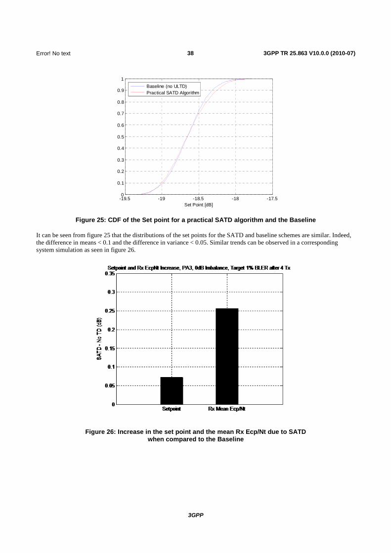
38
3GPP
Error! No text of specified
3GPP TR 25.863 V10.0.0 (2010-07)
-19.5 -19 -18.5 -18 -17.50
0.1
0.2
0.3
0.4
0.5
0.6
0.7
0.8
0.9
1
Set Point [dB]
Baseline (no ULTD)Practical SATD Algorithm
Figure 25: CDF of the Set point for a practical SATD algorithm and the Baseline
It can be seen from figure 25 that the distributions of the set points for the SATD and baseline schemes are similar. Indeed, the difference in means < 0.1 and the difference in variance < 0.05. Similar trends can be observed in a corresponding system simulation as seen in figure 26.
Figure 26: Increase in the set point and the mean Rx Ecp/Nt due to SATD when compared to the Baseline

39
3GPP
Error! No text of specified
3GPP TR 25.863 V10.0.0 (2010-07)
Figure 26 shows that the set point increase is < 0.1 dB whereas the Rx Ecp/Nt increases by 0.26 dB. The trends in a system simulation match the ones seen in the link simulations. Therefore, further modeling of the NodeB Rx loss due to SATD in system simulator, for e.g. adding a back off to the Rx SNR may not necessary for the PA3 channel under the simulation parameters described in table 3 since the increase in the Rx SNR is implicitly captured by the variation of the channel. As noted in section 6.1.4 the Rx performance impact is larger for more stringent BLER requirements (than 1 % residual BLER after the fourth transmission) and for such operating points additional modeling of the NodeB Rx loss due to SATD may be necessary.
5.4 System Performance Evaluation Metrics The following performance measures are considered when evaluating the system performance:
- Average user throughput as a function of cell throughput.
- 10th, 50th and 90th percentile user throughput.
- Average and 90th percentile noise rise levels.
- Average, 10th, 50th and 90th percentile of the UE transmit power.
- Number of antenna switches per second.
- VoIP outage as a function of number of users (*):
· VoIP outage is defined as the percentage of users in outage.
· A VoIP user is said to be in outage when more than 3% of vocoder frames are lost.
The performance measures have previously been summarized in [18].
In addition, for the bursty traffic model, the following performance metrics are considered:
- Average user burst rate.
- 10th percentile user burst rate.
It should be noted that the bursty traffic model employed in this investigation assumed a large file size and offered load levels of 0-1 Mbps. The BLER operating point was 10 % after 1 transmission, which differs from the HARQ operating point for the full buffer simulations in the present document (1 Mbps represents full loading at this operating point but is somewhat lower than full loading at a larger retransmission rate). All UEs were assumed to transmit DPCCH continuously and thus a constant stream of TPC commands was made available to the practical TxD algorithms. A full assessment of bursty traffic performance should consider also small burst sizes, the effect of CPC and the effect of state transitions.
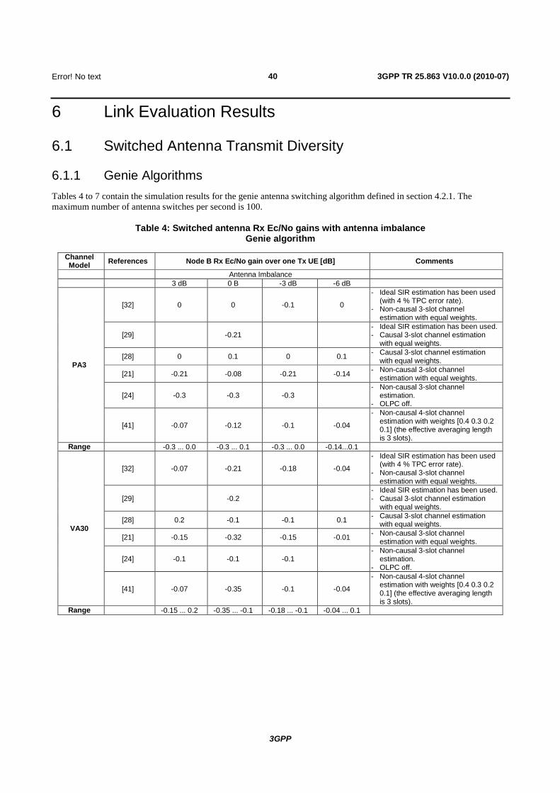
40
3GPP
Error! No text of specified
3GPP TR 25.863 V10.0.0 (2010-07)
6 Link Evaluation Results
6.1 Switched Antenna Transmit Diversity
6.1.1 Genie Algorithms Tables 4 to 7 contain the simulation results for the genie antenna switching algorithm defined in section 4.2.1. The maximum number of antenna switches per second is 100.
Table 4: Switched antenna Rx Ec/No gains with antenna imbalance Genie algorithm
Channel Model References Node B Rx Ec/No gain over one Tx UE [dB] Comments
Antenna Imbalance 3 dB 0 B -3 dB -6 dB
PA3
[32] 0 0 -0.1 0
- Ideal SIR estimation has been used (with 4 % TPC error rate).
- Non-causal 3-slot channel estimation with equal weights.
[29] -0.21 - Ideal SIR estimation has been used. - Causal 3-slot channel estimation
with equal weights.
[28] 0 0.1 0 0.1 - Causal 3-slot channel estimation with equal weights.
[21] -0.21 -0.08 -0.21 -0.14 - Non-causal 3-slot channel estimation with equal weights.
[24] -0.3 -0.3 -0.3 - Non-causal 3-slot channel
estimation. - OLPC off.
[41] -0.07 -0.12 -0.1 -0.04
- Non-causal 4-slot channel estimation with weights [0.4 0.3 0.2 0.1] (the effective averaging length is 3 slots).
Range -0.3 ... 0.0 -0.3 ... 0.1 -0.3 ... 0.0 -0.14...0.1
VA30
[32] -0.07 -0.21 -0.18 -0.04
- Ideal SIR estimation has been used (with 4 % TPC error rate).
- Non-causal 3-slot channel estimation with equal weights.
[29] -0.2 - Ideal SIR estimation has been used. - Causal 3-slot channel estimation
with equal weights.
[28] 0.2 -0.1 -0.1 0.1 - Causal 3-slot channel estimation with equal weights.
[21] -0.15 -0.32 -0.15 -0.01 - Non-causal 3-slot channel estimation with equal weights.
[24] -0.1 -0.1 -0.1 - Non-causal 3-slot channel
estimation. - OLPC off.
[41] -0.07 -0.35 -0.1 -0.04
- Non-causal 4-slot channel estimation with weights [0.4 0.3 0.2 0.1] (the effective averaging length is 3 slots).
Range -0.15 ... 0.2 -0.35 ... -0.1 -0.18 ... -0.1 -0.04 ... 0.1

41
3GPP
Error! No text of specified
3GPP TR 25.863 V10.0.0 (2010-07)
Table 5: Switched antenna Rx Ec/No gains with antenna correlation Genie algorithm
Channel Model References Node B Rx Ec/No gain over one Tx UE [dB] Comments
Antenna Correlation 0 0.3 0.7
PA3
[32] 0 0 0
- Ideal SIR estimation has been used (with 4 % TPC error rate).
- Non-causal 3-slot channel estimation with equal weights.
[29] -0.21 - Ideal SIR estimation has been used. - Causal 3-slot channel estimation with equal
weights.
[28] 0.1 0 0 - Causal 3-slot channel estimation with equal weights.
[21] -0.08 -0.10 -0.13 - Non-causal 3-slot channel estimation with equal weights.
[24] -0.3 - Non-causal 3-slot channel estimation. - OLPC off.
[41] -0.11 -0.11 -0.09 - Non-causal 4-slot channel estimation with
weights [0.4 0.3 0.2 0.1] (the effective averaging length is 3 slots).
Range -0.3 ... 0.1 -0.11 ... 0 -0.13 ...0
VA30
[32] -0.21 -0.17 -0.05
- Ideal SIR estimation has been used (with 4 % TPC error rate).
- Non-causal 3-slot channel estimation with equal weights.
[29] -0.2 - Ideal SIR estimation has been used. - Causal 3-slot channel estimation with equal
weights.
[28] -0.1 -0.3 -0.1 - Causal 3-slot channel estimation with equal weights.
[21] -0.32 -0.27 -0.19 - Non-causal 3-slot channel estimation with equal weights.
[24] -0.1 - Non-causal 3-slot channel estimation. - OLPC off.
[41] -0.35 -0.29 -0.15 - Non-causal 4-slot channel estimation with
weights [0.4 0.3 0.2 0.1] (the effective averaging length is 3 slots).
Range -0.35 ... -0.1 -0.3 ... -0.17 -0.19 ... -0.05

42
3GPP
Error! No text of specified
3GPP TR 25.863 V10.0.0 (2010-07)
Table 6: Switched antenna Tx Ec/No gains with antenna imbalance Genie algorithm
Channel Model References UE Tx Ec/No gain over one Tx UE [dB] Comments
Antenna Imbalance 3 dB 0 dB -3 dB -6 dB
PA3
[32] 4.22 2.41 1.05 0.34
- Ideal SIR estimation has been used (with 4 % TPC error rate).
- Non-causal 3-slot channel estimation with equal weights.
[19] [0.98] - Causal 3-slots channel estimation with equal weights.
[29] 2.46 - SIR estimation has been used. - Causal 3-slot channel estimation
with equal weights.
[28] 4.3 2.7 1.4 0.7 - Causal 3-slot channel estimation with equal weights.
[21] 3.65 1.92 0.65 0.15 - Non-causal 3-slot channel estimation with equal weights.
[24] 3.8 1.8 0.8 - Non-causal 3-slot channel
estimation. - OLPC off.
[41] 4.5 2.7 1.4 0.6
- Non-causal 4-slot channel estimation with weights [0.4 0.3 0.2 0.1] (the effective averaging length is 3 slots).
Range 3.65 ...4.5 1.8 ... 2.7 0.65 ... 1.4 0.15 ... 0.7
VA30
[32] 2.79 0.05 -0.35 -0.08
- Ideal SIR estimation has been used (with 4 % TPC error rate).
- Non-causal 3-slot channel estimation with equal weights.
[19] -0.09 - Causal 3-slots channel estimation with equal weights
[29] 0.09 - Ideal SIR estimation has been used. - Causal 3-slot channel estimation
with equal weights.
[28] 3.0 0.1 -0.2 0.1 - Causal 3-slot channel estimation with equal weights.
[21] 2.71 -0.15 -0.29 -0.02 - Non-causal 3-slot channel estimation with equal weights.
[24] 3.4 0.8 0.4 - Non-causal 3-slot channel
estimation. - OLPC off.
[41] 2.78 -0.05 -0.23 -0.05
- Non-causal 4-slot channel estimation with weights [0.4 0.3 0.2 0.1] (the effective averaging length is 3 slots).
Range 2.71 ... 3.4 -0.15 ... 0.8 -0.35... 0.4 -0.08 ... 0.1

43
3GPP
Error! No text of specified
3GPP TR 25.863 V10.0.0 (2010-07)
Table 7: Switched antenna Tx Ec/No gains with antenna correlation Genie algorithm
Channel Model References UE Tx Ec/No gain over one Tx UE [dB] Comments
Antenna Correlation 0 0.3 0.7
PA3
[32] 2.41 2.32 1.81
- Ideal SIR estimation has been used (with 4 % TPC error rate).
- Non-causal 3-slot channel estimation with equal weights.
[19] [0.98] - Causal 3-slots channel estimation with equal weights.
[29] 2.46 - Ideal SIR estimation has been used. - Causal 3-slot channel estimation with equal
weights.
[28] 2.7 2.6 2.0 - Causal 3-slot channel estimation with equal weights.
[21] 1.92 1.86 1.39 - Non-causal 3-slot channel estimation with equal weights.
[24] 1.8 - Non-causal 3-slot channel estimation. - OLPC off.
[41] 2.68 2.55 2.0 - Non-causal 4-slot channel estimation with
weights [0.4 0.3 0.2 0.1] (the effective averaging length is 3 slots).
Range 1.8 ... 2.7 1.86 ... 2.6 1.39 ... 2.0
VA30
[32] 0.05 0.06 0.09
- Ideal SIR estimation has been used (with 4 % TPC error rate).
- Non-causal 3-slot channel estimation with equal weights.
[19] -0.09 - Causal 3-slots channel estimation with equal weights.
[29] 0.09 - Ideal SIR estimation has been used. - Causal 3-slot channel estimation with equal
weights.
[28] 0.1 0 0.1 - Causal 3-slot channel estimation with equal weights.
[21] -0.15 -0.08 -0.03 - Non-causal 3-slot channel estimation with equal weights.
[24] 0.8 - Non-causal 3-slot channel estimation. - OLPC off.
[41] -0.05 0 0.04 - Non-causal 4-slot channel estimation with
weights [0.4 0.3 0.2 0.1] (the effective averaging length is 3 slots).
Range -0.15 ... 0.8 -0.08 ... 0.06 -0.03 ... 0.1
Tables 8 to 11 contain the simulation results for the genie antenna switching algorithm defined in section 4.3.1 with different settings for the maximum number of antenna switches per second. The results have been contributed in [36].
Table 8: Switched antenna Rx Ec/No gains with antenna imbalance Genie algorithm; Maximum Switch Frequency - 25 Hz, 50 Hz
Antenna Switch Frequency
Channel Model
Node B Rx Ec/No gain over one Tx UE [dB] Comments
Antenna Imbalance 3 dB 0 dB -3 dB -6 dB
100 PA3 0 0 -0.1 0 - Ideal SIR estimation has been used
(with 4 % TPC error rate). - Non-causal 3-slot channel estimation
with equal weights.
VA30 -0.07 -0.21 -0.18 -0.04
50 PA3 -0.10 -0.10 0.00 -0.10 VA30 -0.07 -0.15 -0.04 -0.06
25 PA3 -0.20 VA30 -0.07

44
3GPP
Error! No text of specified
3GPP TR 25.863 V10.0.0 (2010-07)
Table 9: Switched antenna Rx Ec/No gains with antenna correlation Genie algorithm; Maximum Switch Frequency - 25 Hz, 50 Hz
Antenna Switch Frequency
Channel Model
Node B Rx Ec/No gain over one Tx UE [dB] Comments
Antenna Correlation 0 0.3 0.7
100 PA3 0 0 0 - Ideal SIR estimation has been
used (with 4 % TPC error rate). - Non-causal 3-slot channel
estimation with equal weights.
VA30 -0.21 -0.17 -0.05
50 PA3 -0.10 0.00 -0.10 VA30 -0.15 -0.13 -0.04
25 PA3 -0.20 VA30 -0.07
Table 10: Switched antenna Tx Ec/No gains with antenna imbalance Genie algorithm; Maximum Switch Frequency - 25 Hz, 50 Hz
Antenna Switch Frequency
Channel Model UE Tx Ec/No gain over one Tx UE [dB] Comments
Antenna Imbalance 3 dB 0 dB -3 dB -6 dB
100 PA3 4.22 2.41 1.05 0.34 - Ideal SIR estimation has been used
(with 4 % TPC error rate). - Non-causal 3-slot channel estimation
with equal weights.
VA30 2.79 0.05 -0.35 -0.08
50 PA3 4.14 2.35 1.08 0.23 VA30 2.58 0.08 -0.45 -0.21
25 PA3 1.67 VA30 0.06
Table 11: Switched antenna Tx Ec/No gains with antenna correlation Genie algorithm; Maximum Switch Frequency - 25 Hz, 50 Hz
Antenna Switch Frequency
Channel Model UE Tx Ec/No gain over one Tx UE [dB] Comments
Antenna Correlation 0 0.3 0.7
100 PA3 2.41 2.32 1.81 - Ideal SIR estimation has been used
(with 4 % TPC error rate). - Non-causal 3-slot channel
estimation with equal weights.
VA30 0.05 0.06 0.09
50 PA3 2.35 2.28 1.69 VA30 0.08 0.07 0.09
25 PA3 1.67 VA30 0.06
6.1.2 Practical Algorithms Tables 12 to 15 contain the simulation results for the practical antenna switching algorithm defined in section 4.3.1 with forced switching after 14 frames. The maximum number of antenna switches per second is 100.

45
3GPP
Error! No text of specified
3GPP TR 25.863 V10.0.0 (2010-07)
Table 12: Switched antenna Rx Ec/No gains with antenna imbalance Practical algorithm
Channel Model References Node B Rx Ec/No gain over one Tx UE [dB] Comments
Antenna Imbalance 3 dB 0 dB -3 dB -6 dB
PA3
[21] -0.36 -0.28 -0.36 -0.72 - Non-causal 3-slot channel estimation with equal weights.
[41] -0.53 -0.41 -0.45 -0.73
- Non-causal 4-slot channel estimation with weights [0.4 0.3 0.2 0.1] (the effective averaging length is 3 slots).
[36] -0.40 -0.40 -0.40 -0.70
- Ideal SIR estimation has been used (with 4 % TPC error rate).
- Non-causal 3-slot channel estimation with equal weights.
[24] -0.4 -0.4 -0.4 - OLPC off. - Non-causal 3-slot channel
estimation. Range -0.53 ... -0.35 -0.41 ... -0.24 -0.45 ... -0.32 -0.73 ... -0.55
VA30
[21] -0.31 -0.21 -0.31 -0.58 - Non-causal 3-slot channel estimation with equal weights.
[41] -0.23 -0.10 -0.26 -0.47
- Non-causal 4-slot channel estimation with weights [0.4 0.3 0.2 0.1] (the effective averaging length is 3 slots).
[36] -0.10 -0.08 -0.08 -0.41
- Ideal SIR estimation has been used (with 4 % TPC error rate).
- Non-causal 3-slot channel estimation with equal weights.
[24] -0.1 -0.1 -0.1 - OLPC off. - Non-causal 3-slot channel
estimation. Range -0.31 ...-0.1 -0.21 ... -0.1 -0.31 ... -0.1 -0.58…-0.41

46
3GPP
Error! No text of specified
3GPP TR 25.863 V10.0.0 (2010-07)
Table 13: Switched antenna Rx Ec/No gains with antenna correlation Practical algorithm
Channel Model
References Node B Rx Ec/No gain over one Tx UE [dB] Comments
Antenna Correlation 0 0.3 0.7
PA3
[21] -0.28 -0.26 -0.20 - Non-causal 3-slot channel estimation with equal weights.
[41] -0.41 -0.29 -0.26 - Non-causal 4-slot channel estimation with
weights [0.4 0.3 0.2 0.1] (the effective averaging length is 3 slots).
[36] -0.40 -0.30 -0.20
- Ideal SIR estimation has been used (with 4 % TPC error rate).
- Non-causal 3-slot channel estimation with equal weights.
[24] -0.4 - OLPC off. - Non-causal 3-slot channel estimation.
Range -0.41 ... -0.28 -0.30 …-0.26 -0.26 …-0.20
VA30
[21] -0.32 -0.27 -0.19 - Non-causal 3-slot channel estimation with equal weights.
[41] -0.10 -0.12 -0.04 - Non-causal 4-slot channel estimation with
weights [0.4 0.3 0.2 0.1] (the effective averaging length is 3 slots).
[36] -0.08 -0.11 0.02
- Ideal SIR estimation has been used (with 4 % TPC error rate).
- Non-causal 3-slot channel estimation with equal weights.
[24] -0.1 - OLPC off. - Non-causal 3-slot channel estimation.
Range -0.32 ... -0.08 -0.27 …-0.11 -0.19 …0.02
Table 14: Switched antenna Tx Ec/No gains with antenna imbalance Practical algorithm
Channel Model References UE Tx Ec/No gain over one Tx UE [dB] Comments
Antenna Imbalance 3 dB 0 dB -3 dB -6 dB
PA3
[21] 2.85 0.99 -0.15 -1.11 - Non-causal 3-slot channel estimation with equal weights.
[41] 3.13 1.42 0.10 -0.76 - Non-causal 4-slot channel estimation
with weights [0.4 0.3 0.2 0.1] (the effective averaging length is 3 slots).
[36] 2.93 1.03 -0.09 -1.25
- Ideal SIR estimation has been used (with 4 % TPC error rate).
- Non-causal 3-slot channel estimation with equal weights.
[24] 3.2 0.4 0.2 - OLPC off. - Non-causal 3-slot channel
estimation. Range 2.81 ... 3.2 0.4 ... 1.42 -0.15 ... 0.2 -1.25 ... -0.76
VA30
[21] 2.06 -0.15 -0.94 -1.17 - Non-causal 3-slot channel estimation with equal weights.
[41] 2.12 0.02 -0.89 -1.09 - Non-causal 4-slot channel estimation
with weights [0.4 0.3 0.2 0.1] (the effective averaging length is 3 slots).
[36] 2.23 -0.02 -0.69 -1.03
- Ideal SIR estimation has been used (with 4 % TPC error rate).
- Non-causal 3-slot channel estimation with equal weights.
[24] 3.1 0.2 0.1 - OLPC off. - Non-causal 3-slot channel
estimation. Range 2.06 ... 3.1 -0.15 ... 0.2 -0.94 ... 0.1 -1.17 ... -1.03

47
3GPP
Error! No text of specified
3GPP TR 25.863 V10.0.0 (2010-07)
Table 15: Switched antenna Tx Ec/No gains with antenna correlation Practical algorithm
Channel Model References UE Tx Ec/No gain over one Tx UE [dB] Comments
Antenna Correlation 0 0.3 0.7
PA3
[21] 0.99 1.00 0.63 - Non-causal 3-slot channel estimation with equal weights.
[41] 1.42 1.45 1.02 - Non-causal 4-slot channel estimation with
weights [0.4 0.3 0.2 0.1] (the effective averaging length is 3 slots).
[36] 1.03 1.21 0.76
- Ideal SIR estimation has been used (with 4 % TPC error rate).
- Non-causal 3-slot channel estimation with equal weights.
[24] 0.4 - OLPC off. - Non-causal 3-slot channel estimation.
Range 0.4 ... 1.42 1.00 … 1.45 0.63 … 1.02
VA30
[21] -0.15 -0.08 -0.03 - Non-causal 3-slot channel estimation with equal weights.
[41] 0.02 0 0.02 - Non-causal 4-slot channel estimation with
weights [0.4 0.3 0.2 0.1] (the effective averaging length is 3 slots).
[36] -0.02 -0.05 0.01
- Ideal SIR estimation has been used (with 4 % TPC error rate).
- Non-causal 3-slot channel estimation with equal weights.
[24] 0.2 - OLPC off. - Non-causal 3-slot channel estimation.
Range -0.15 ... 0.2 -0.08 … 0 -0.03 …0.02
Tables 16 to 19 contain the simulation results for for the practical antenna switching algorithm defined in section 4.3.1 with forced switching after 14 frames for different settings for the maximum number of antenna switches per second. The results have been contributed in [36].
Table 16: Switched antenna Rx Ec/No gains with antenna imbalance Practical algorithm; Maximum Switch Frequency - 25 Hz, 50 Hz
Antenna Switch Frequency
Channel Model
Node B Rx Ec/No gain over one Tx UE [dB] Comments
Antenna Imbalance 3 dB 0 dB -3 dB -6 dB
100 PA3 -0.40 -0.40 -0.40 -0.70 - Ideal SIR estimation has been used
(with 4 % TPC error rate). - Non-causal 3-slot channel estimation
with equal weights.
VA30 -0.10 -0.08 -0.08 -0.41
50 PA3 -0.30 -0.30 -0.40 -0.40 VA30 -0.04 -0.04 -0.08 -0.24
25 PA3 -0.20 VA30 0.05

48
3GPP
Error! No text of specified
3GPP TR 25.863 V10.0.0 (2010-07)
Table 17: Switched antenna Rx Ec/No gains with antenna correlation Practical algorithm; Maximum Switch Frequency - 25 Hz, 50 Hz
Antenna Switch Frequency
Channel Model Node B Rx Ec/No gain over one Tx UE [dB] Comments
Antenna Correlation 0 0.3 0.7
100 PA3 -0.40 -0.30 -0.20 - Ideal SIR estimation has been
used (with 4 % TPC error rate). - Non-causal 3-slot channel
estimation with equal weights.
VA30 -0.08 -0.11 0.02
50 PA3 -0.30 -0.20 -0.10 VA30 -0.04 -0.08 -0.02
25 PA3 -0.20 VA30 0.05
Table 18: Switched antenna Tx Ec/No gains with antenna imbalance Practical algorithm; Maximum Switch Frequency - 25 Hz, 50 Hz
Antenna Switch Frequency
Channel Model UE Tx Ec/No gain over one Tx UE [dB] Comments
Antenna Imbalance 3 dB 0 dB -3 dB -6 dB
100 PA3 2.93 1.03 -0.09 -1.25 - Ideal SIR estimation has been
used (with 4 % TPC error rate). - Non-causal 3-slot channel
estimation with equal weights.
VA30 2.23 -0.02 -0.69 -1.03
50 PA3 2.46 0.76 -0.70 -1.61 VA30 2.31 0.00 -0.80 -1.17
25 PA3 0.22 VA30 0.05
Table 19: Switched antenna Tx Ec/No gains with antenna correlation Practical algorithm; Maximum Switch Frequency - 25 Hz, 50 Hz
Antenna Switch Frequency
Channel Model UE Tx Ec/No gain over one Tx UE [dB] Comments
Antenna Correlation 0 0.3 0.7
100 PA3 1.03 1.21 0.76 - Ideal SIR estimation has been used
(with 4 % TPC error rate). - Non-causal 3-slot channel estimation
with equal weights.
VA30 -0.02 -0.05 0.01
50 PA3 0.76 0.68 0.51 VA30 0.00 -0.08 -0.06
25 PA3 0.22 VA30 0.05

49
3GPP
Error! No text of specified
3GPP TR 25.863 V10.0.0 (2010-07)
Tables 20 to 23 contain the simulation results for the practical antenna switching algorithm defined in section 4.3.1 with forced switching after 4 frames. The maximum number of antenna switches per second is 100.
Table 20: Switched antenna Rx Ec/No gains with antenna imbalance Practical algorithm
Channel Model References Node B Rx Ec/No gain over one Tx UE [dB] Antenna Imbalance 3 dB 0 dB -3 dB -6 dB
PA3 [23] -1.2 -0.1 -0.8 [20] -1.3 -1 -1.3 -2.1 [32] -1.01 -0.7 -0.94 -1.85
Range -1.3 ... -1.01 -1.0 ... -0.1 -1.3 ... -0.8 -2.1 ... -1.85
VA30 [23] -0.8 -0.2 -0.5 [20] -0.7 -0.4 -0.7 -1.4 [32] -0.54 -0.22 -0.49 -1.27
Range -0.8 ... -0.54 -0.4 ... -0.2 -0.7 ... -0.49 -1.4 ... -1.27
Table 21: Switched antenna Rx Ec/No gains with antenna correlation Practical algorithm
Channel Model References Node B Rx Ec/No gain over one Tx UE [dB] Antenna Correlation 0 0.3 0.7
PA3 [23] -0.1 [20] -1 -1 [32] -0.7 -0.7 -0.4
Range -1.0 ... -0.1 -1.0 ... -0.7 -0.4
VA30 [23] -0.2 [20] -0.4 -0.3 [32] -0.22 -0.17 -0.14
Range -0.4 ... -0.2 -0.3 ... -0.17 -0.14
Table 22: Switched antenna Tx Ec/No gains with antenna imbalance Practical algorithm
Channel Model References UE Tx Ec/No gain over one Tx UE [dB] Antenna Imbalance 3 dB 0 dB -3 dB -6 dB
PA3 [23] 3 1.8 0 [20] 2 0.5 -1 -2.5 [32] 2.58 1.08 -0.45 -2.12
Range 2.0 ... 3.0 0.5 ... 1.8 -1 ... 0 -2.5 ... -2.12
VA30 [23] 2.5 0.2 -0.2 [20] 1.4 -0.2 -1.6 -2.7 [32] 1.62 -0.08 -1.37 -2.53
Range 1.4 ... 2.5 -0.2 ... 0.2 -1.6 ... -0.2 -2.7 ... -2.53

50
3GPP
Error! No text of specified
3GPP TR 25.863 V10.0.0 (2010-07)
Table 23: Switched antenna Tx Ec/No gains with antenna correlation Practical algorithm
Channel Model References UE Tx Ec/No gain over one Tx UE [dB] Antenna Correlation 0 0.3 0.7
PA3 [23] 1.8 [20] 0.5 0.5 [32] 1.08 1.04 0.79
Range 0.5 ... 1.8 0.5 ... 1.04 0.79
VA30 [23] 0.2 [20] -0.2 -0.1 [32] -0.08 -0.08 -0.01
Range -0.2 ... 0.2 -0.1 ... -0.08 -0.01
6.1.3 Impact of Realistic E-DPCCH Decoding on Switched Antenna Transmit Diversity
The link simulation results presented above have been performed with ideal E-DPCCH decoding. In this section the performance with realistic E-DPCCH decoding are presented for both genie and practical switched antenna transmit diversity algorithms based on the link evaluation in [68].
Tables 23a to 23d contain the simulation results for the genie antenna switching algorithm defined in section 4.2.1 with realistic E-DPCCH decoding. The maximum number of antenna switches per second is 100.
Table 23a: Switched antenna Rx Ec/No gains with antenna imbalance Genie algorithm with E-DPCCH decoding
Channel Model Node B Rx Ec/No gain over one Tx UE [dB] Comments Antenna Imbalance 3 dB 0 dB -3 dB
PA3 -0.02 0 0 - Non-causal 4-slot channel estimation with weights [0.4 0.3 0.2 0.1] (the effective averaging length is 3 slots). VA30 -0.13 -0.33 -0.08
Table 23b: Switched antenna Rx Ec/No gains with antenna correlation Genie algorithm with E-DPCCH decoding
Channel Model Node B Rx Ec/No gain over one Tx UE [dB] Comments Antenna Correlation 0 0.3 0.7
PA3 0 0 0 - Non-causal 4-slot channel estimation with weights [0.4 0.3 0.2 0.1] (the effective averaging length is 3 slots). VA30 -0.33 -0.28 -0.21
Table 23c: Switched antenna Tx Ec/No gains with antenna imbalance Genie algorithm with E-DPCCH decoding
Channel Model UE Tx Ec/No gain over one Tx UE [dB] Comments Antenna Imbalance 3 dB 0 dB -3 dB
PA3 4.54 2.76 1.47 - Non-causal 4-slot channel estimation with weights [0.4 0.3 0.2 0.1] (the effective averaging length is 3 slots). VA30 2.72 -0.02 -0.2

51
3GPP
Error! No text of specified
3GPP TR 25.863 V10.0.0 (2010-07)
Table 23d: Switched antenna Tx Ec/No gains with antenna correlation Genie algorithm with E-DPCCH decoding
Channel Model UE Tx Ec/No gain over one Tx UE [dB] Comments Antenna Correlation 0 0.3 0.7
PA3 2.76 2.65 2.07 - Non-causal 4-slot channel estimation with weights [0.4 0.3 0.2 0.1] (the effective averaging length is 3 slots). VA30 -0.02 0.007 -0.004
Tables 23e to 23h contain the simulation results for the practical antenna switching algorithm defined in section 4.3.1 with forced switching after 14 frames with realistic E-DPCCH decoding. The maximum number of antenna switches per second is 100.
Table 23e: Switched antenna Rx Ec/No gains with antenna imbalance Practical algorithm with E-DPCCH decoding
Channel Model Node B Rx Ec/No gain over one Tx UE [dB] Comments Antenna Imbalance 3 dB 0 dB -3 dB
PA3 -0.41 -0.23 -0.39 - Non-causal 4-slot channel estimation with weights [0.4 0.3 0.2 0.1] (the effective averaging length is 3 slots). VA30 -0.28 -0.12 -0.18
Table 23f: Switched antenna Rx Ec/No gains with antenna correlation Practical algorithm with E-DPCCH decoding
Channel Model Node B Rx Ec/No gain over one Tx UE [dB] Comments Antenna Correlation 0 0.3 0.7
PA3 -0.23 -0.26 -0.14 - Non-causal 4-slot channel estimation with weights [0.4 0.3 0.2 0.1] (the effective averaging length is 3 slots). VA30 -0.12 -0.14 -0.09
Table 23g: Switched antenna Tx Ec/No gains with antenna imbalance Practical algorithm with E-DPCCH decoding
Channel Model UE Tx Ec/No gain over one Tx UE [dB] Comments Antenna Imbalance 3 dB 0 dB -3 dB
PA3 3.22 1.62 0.15 - Non-causal 4-slot channel estimation with weights [0.4 0.3 0.2 0.1] (the effective averaging length is 3 slots).
VA30 2.09 -0.007 -0.81
Table 23h: Switched antenna Tx Ec/No gains with antenna correlation Practical algorithm with E-DPCCH decoding
Channel Model UE Tx Ec/No gain over one Tx UE [dB] Comments Antenna Correlation 0 0.3 0.7
PA3 1.62 1.49 1.15 - Non-causal 4-slot channel estimation with weights [0.4 0.3 0.2 0.1] (the effective averaging length is 3 slots). VA30 -0.007 -0.03 -0.02

52
3GPP
Error! No text of specified
3GPP TR 25.863 V10.0.0 (2010-07)
6.1.4 HS-DPCCH Performance in Soft Handover with Switched Antenna Transmit Diversity
6.1.4.1 Notation
GTx1->A: The antenna gain for the link from Antenna 1 (Tx1) to A which is the serving NodeB.
GTx2->A: The antenna gain for the link from Antenna 2 (Tx2) to A which is the serving NodeB.
GTx1->B: The antenna gain for the link from Antenna 1 (Tx1) to B which is the non-serving NodeB.
GTx2->B: The antenna gain for the link from Antenna 2 (Tx2) to B which is the non-serving NodeB.
IA->B: The imbalance between the two links from UE Antenna 1 to A and from UE Antenna 1 to B where A and B are the two NodeB's in the active set. The UE is in soft handover. In other words IA->B = GTx1-
>A - GTx1->B.
These variables along with the simulation framework are shown in figure 27.
Figure 27: Simulation framework where the UE is in soft handover with Serving NodeB A and Non-Serving NodeB B
The imbalance between the antennas (Tx1 and Tx2) is different for the links to the serving and non-serving NodeB's. They are indicated below:
IUE->A = GTx1->A - GTx2->A: The imbalance between the two transmit antennas Tx1 and Tx2 for the radio link to the serving NodeB A.
IUE->B = GTx1->B - GTx2->B: The imbalance between the two transmit antennas Tx1 and Tx2 for the radio link to the non-serving NodeB B.

53
3GPP
Error! No text of specified
3GPP TR 25.863 V10.0.0 (2010-07)
It is assumed in the simulation that the path loss to the serving and non-serving NodeB's are the same. Therefore:
IA->B = GTx1->A - GTx1->B = 0 dB.
6.1.4.2 HS-DPCCH Performance
Table 24 shows the HS-DPCCH ACK/NACK Miss detection and Decoding error rate performance when SATD is applied at the UE. In this simulation framework, the UE is in soft handover with two cells in the active set.
Table 24: HS-DPCCH ACK/NACK performance due to SATD in SHO
SATD HS-DPCCH ACK/NACK miss detection and decoding error rate [%]@ C/P=4 dB (Baseline value, SATD value)
SHO Link Imbalance
IA->B = 0 dB
Serving Cell Imbalance IUE->A IUE->A = 0 dB
Non Serving Cell Imbalance IUE->B IUE->B = 0 dB IUE->B = 3 dB IUE->B = -3 dB
PA3 (0.8 %, 0.8 %)† (0.8 %, 2 %) (0.8 %, 0.55 %) VA30 (0.02 %, 0.03 %) (0.02 %, 0.02 %) (0.02 %, 0.01 %) † The data format in the table is (Baseline value, SATD value).
Table 25 shows the HS-DPCCH CQI Decoding error rate performance when SATD is applied at the UE. In this simulation framework, the UE is in soft handover with two cells in the active set.
Table 25: HS-DPCCH CQI performance loss due to SATD in SHO
SATD HS-DPCCH CQI decoding error rate [%]@ C/P=0 dB (Baseline value, SATD value)
SHO Link Imbalance
IA->B = 0 dB.
Serving Cell Imbalance IUE->A IUE->A = 0 dB
Non Serving Cell Imbalance IUE->B IUE->B = 0 dB IUE->B = 3 dB IUE->B = -3 dB
PA3 (1 %, 1.2 %)† (1 %, 2.6 %) (1 %, 0.9 %) VA30 (0.06 %, 0.08 %) (0.06 %, 0.06 %) (0.06 %, 0.06 %) † The data format in the table is (Baseline value, SATD value).
6.1.5 Sensitivity with respect to the BLER operating point The evaluations presented above have been performed at an operating point where the residual BLER target after the 4th transmission is 1 %. In this section we therefore evaluate the relative gain in Tx and Rx Ec/No as a function of different BLER targets (after the first transmission). Note that the evaluation only is performed for the case where the antenna imbalance is 0 dB.
Table 26 presents the relative gain in Tx Ec/N0 and table 27 presents the relative gain in Rx Ec/No for different BLER levels for the switched antenna diversity algorithms.

54
3GPP
Error! No text of specified
3GPP TR 25.863 V10.0.0 (2010-07)
Table 26: Results showing Tx Ec/No relative gains with respect to reference case without Tx diversity for a scenario without transmit antenna correlation as a function
of the BLER target after first transmission [21]
BLER@ first transmission [%]
2 5 10 20 30 40 50
PA3 SATD Genie 2.06 1.83 1.92 2.05 1.91 1.89 1.94 SATD Prac 0.65 0.97 0.96 1.21 0.99 1 1.18
VA30 SATD Genie -1.4 -0.5 -0.25 -0.23 -0.18 -0.08 -0.08 SATD Prac -0.52 -0.41 -0.26 -0.22 -0.22 -0.05 -0.1
Table 27: Results showing Rx Ec/No relative gains with respect to reference case without Tx diversity for a scenario without transmit antenna correlation as a function
of the BLER target after first transmission [21]
BLER@ first transmission [%]
2 5 10 20 30 40 50
PA3 SATD Genie 0.02 -0.08 -0.03 -0.05 -0.08 -0.19 -0.17 SATD Prac -0.68 -0.41 -0.28 -0.26 -0.34 -0.35 -0.17
VA30 SATD Genie -1.55 -0.7 -0.43 -0.41 -0.36 -0.30 -0.31 SATD Prac -0.6 -0.42 -0.37 -0.3 -0.27 -0.17 -0.21

55
3GPP
Error! No text of specified
3GPP TR 25.863 V10.0.0 (2010-07)
6.2 Beamforming Transmit Diversity
6.2.1 Genie Algorithms Tables 28 to 31 contain the simulation results for the genie beamforming algorithm defined in section 4.2.2.
Table 28: Beamforming Rx Ec/No gains with antenna imbalance Genie algorithm
Channel Model References Node B Rx Ec/No gain over one Tx UE [dB] Comments
Antenna Imbalance 3 dB 0 dB -3 dB -6 dB
PA3
[25] -0.1 -0.1 -0.1 - OLPC off. - Non-causal 3-slot channel estimation.
[22] 0.0 0.01 0.00 -0.04 - Non-causal 3-slot channel estimation with equal weights.
[34] 0.2
- Ideal SIR estimation has been used (with 4 % TPC error rate).
- Non-causal 3-slot channel estimation with equal weights.
[27] -0.1 - Non-causal 3-slot channel estimation with equal weights.
[30] -0.02 0.05 0.05 - Causal 3-slot channel estimation with equal weights.
[28] 0.0 0.1 0.1 0.1 - Causal 3-slot channel estimation with equal weights.
[42] 0.04 0 0 0 - Non-causal 4-slot channel estimation
with weights [0.4 0.3 0.2 0.1] (the effective averaging length is 3 slots).
Range -0.1… 0.04 -0.1… 0.2 -0.1…
0.1 -0.04…
0.1
VA30
[25] -0.2 -0.2 -0.2 - OLPC off. - Non-causal 3-slot channel estimation
[22] -0.08 -0.03 -0.08 0.08 - Non-causal 3-slot channel estimation with equal weights.
[34] -0.02
- Ideal SIR estimation has been used (with 4 % TPC error rate). - Non-causal 3-slot channel estimation with equal weights.
[27] -0.20 - Non-causal 3-slot channel estimation with equal weights.
[30] -0.21 - Causal 3-slot channel estimation with equal weights.
[28] 0.2 0.2 0.2 0.2 - Causal 3-slot channel estimation with equal weights.
[42] -0.24 0 0.07 0.12 - Non-causal 4-slot channel estimation with weights [0.4 0.3 0.2 0.1] (the effective averaging length is 3 slots).
Range -0.24… 0.2
-0.21… 0.2
-0.2… 0.2
0.08… 0.2
Table 29: Beamforming Rx Ec/No gains with Tx antenna correlation. Genie algorithm
Channel Model References Node B Rx Ec/No gain over
one Tx UE [dB] Comments
Tx Antenna Correlation

56
3GPP
Error! No text of specified
3GPP TR 25.863 V10.0.0 (2010-07)
0 0.3 0.7
PA3
[25] -0.1 - OLPC off. - Non-causal 3-slot channel estimation.
[22] 0.01 0.07 0.08 - Non-causal 3-slot channel estimation with equal weights.
[42] 0 0 0 - Non-causal 4-slot channel estimation with
weights [0.4 0.3 0.2 0.1] (the effective averaging length is 3 slots).
[34] 0.2
- Ideal SIR estimation has been used (with 4 % TPC error rate).
- Non-causal 3-slot channel estimation with equal weights.
[27] -0.1 0.1 - Non-causal 3-slot channel estimation with equal weights.
[30] 0.05 0.01 - Causal 3-slot channel estimation with equal weights.
[28] 0.1 0.1 0.1 - Causal 3-slot channel estimation with equal weights.
Range -0.1… 0.2 0.01… 0.1 0.08… 0.1
VA30
[25] -0.2 - OLPC off. - Non-causal 3-slot channel estimation.
[22] -0.03 0.0 -0.01 - Non-causal 3-slot channel estimation with equal weights.
[42] 0 -0.03 0.02 - Non-causal 4-slot channel estimation with
weights [0.4 0.3 0.2 0.1] (the effective averaging length is 3 slots).
[34] -0.02
- Ideal SIR estimation has been used (with 4 % TPC error rate).
- Non-causal 3-slot channel estimation with equal weights.
[27] -0.2 -0.3 - Non-causal 3-slot channel estimation with equal weights.
[30] -0.21 -0.13 - Causal 3-slot channel estimation with equal weights.
[28] 0.2 0.1 0.2 - Causal 3-slot channel estimation with equal weights.
Range -0.21… 0.2
-0.3… 0.1 -0.01… 0.2

57
3GPP
Error! No text of specified
3GPP TR 25.863 V10.0.0 (2010-07)
Table 30: Beamforming Tx Ec/No gains with antenna imbalance Genie algorithm
Channel Model References UE Tx Ec/No gain over one Tx UE [dB] Comments
Antenna Imbalance 3 dB 0 dB -3 dB -6 dB
PA3
[25] 4.6 2.8 1.6 - OLPC off. - Non-causal 3-slot channel
estimation.
[22] 4.63 3.01 1.63 0.47 - Non-causal 3-slot channel estimation with equal weights.
[42] 5.45 3.78 2.38 1.19
- Non-causal 4-slot channel estimation with weights [0.4 0.3 0.2 0.1] (the effective averaging length is 3 slots).
[34] 3.21
- Ideal SIR estimation has been used (with 4 % TPC error rate).
- Non-causal 3-slot channel estimation with equal weights.
[27] 3.5 - Non-causal 3-slot channel estimation with equal weights.
[19] 2.24 - Causal 3-slot channel estimation with equal weights.
[30] 5.21 3.68 2.31 - Causal 3-slot channel estimation with equal weights.
[28] 5.0 3.6 2.2 1.1 - Causal 3-slot channel estimation with equal weights.
Range 4.6… 5.45
2.24… 3.78
1.6… 2.38
0.47… 1.19
VA30
[25] 2.8 1.0 -0.2 - OLPC off. - Non-causal 3-slot channel
estimation.
[22] 3.19 1.56 0.19 -0.65 - Non-causal 3-slot channel estimation with equal weights.
[42] 2.72 1.41 0.21 -0.7
- Non-causal 4-slot channel estimation with weights [0.4 0.3 0.2 0.1] (the effective averaging length is 3 slots).
[34] 1.49
- Ideal SIR estimation has been used (with 4 % TPC error rate).
- Non-causal 3-slot channel estimation with equal weights.
[27] 1.8 - Non-causal 3-slot channel estimation with equal weights.
[19] 1.22 - Causal 3-slot channel estimation with equal weights
[30] 1.41 - Causal 3-slot channel estimation with equal weights.
[28] 3.4 1.8 0.5 -0.5 - Causal 3-slot channel estimation with equal weights.
Range 2.8… 3.4 1.0… 1.8 -0.2… 0.5
-0.65… -0.5

58
3GPP
Error! No text of specified
3GPP TR 25.863 V10.0.0 (2010-07)
Table 31: Beamforming Tx Ec/No gains with Tx antenna correlation Genie algorithm
Channel Model References UE Tx Ec/No gain over one Tx UE [dB] Comments
Tx Antenna Correlation 0 0.3 0.7
PA3
[25] 2.8 - OLPC off. - Non-causal 3-slot channel estimation.
[22] 3.01 3.11 3.17 - Non-causal 3-slot channel estimation with equal weights.
[42] 3.78 3.69 3.49 - Non-causal 4-slot channel estimation
with weights [0.4 0.3 0.2 0.1] (the effective averaging length is 3 slots).
[34] 3.21
- Ideal SIR estimation has been used (with 4 % TPC error rate).
- Non-causal 3-slot channel estimation with equal weights.
[27] 3.5 3.5 - Non-causal 3-slot channel estimation with equal weights.
[19] 2.24 - Causal 3-slot channel estimation with equal weights
[30] 3.68 3.39 - Causal 3-slot channel estimation with equal weights.
[28] 3.6 3.6 3.4 - Causal 3-slot channel estimation with equal weights.
Range 2.24… 3.78
3.11… 3.69 3.17… 3.49
VA30
[25] 1.0 - OLPC off. - Non-causal 3-slot channel estimation.
[22] 1.56 1.75 2.37 - Non-causal 3-slot channel estimation with equal weights.
[42] 1.41 1.54 2.32 - Non-causal 4-slot channel estimation
with weights [0.4 0.3 0.2 0.1] (the effective averaging length is 3 slots).
[34] 1.49
- Ideal SIR estimation has been used (with 4 % TPC error rate).
- Non-causal 3-slot channel estimation with equal weights.
[27] 1.8 1.9 - Non-causal 3-slot channel estimation with equal weights.
[19] 1.22 - Causal 3-slot channel estimation with equal weights.
[30] 1.41 2.06 - Causal 3-slot channel estimation with equal weights.
[28] 1.8 1.9 2.6 - Causal 3-slot channel estimation with equal weights.
Range 1.0… 1.8 1.54… 2.06 2.32… 2.6
6.2.2 Practical Algorithms Tables 32 to 36 contain the simulation results for the practical beamforming transmit diversity (BFTD) algorithms 1, 2 and 3 defined in section 4.3.2. Unless explicitly stated, the Practical BFTD Algorithm 2 assumes an asymmetric phase implementation. Additionally, for these results, the Rx antenna correlation = 0.
Tables 34 and 37 contain the simulation results for the practical beamforming algorithm transmit diversity transmit diversity (BFTD) algorithm 2 defined in Section 4.3.2 with symmetric and asymmetric phase implementations. The Tx and Rx antenna correlations for these results = 0.3.

59
3GPP
Error! No text of specified
3GPP TR 25.863 V10.0.0 (2010-07)
Table 32: Beamforming Rx Ec/No gains with antenna imbalance Practical algorithm
Channel Model References Node B Rx Ec/No gain over one Tx UE [dB] Comments
Antenna Imbalance 3 dB 0 dB -3 dB -6 dB
PA3
[38] -1.2 -0.9 -0.7 -0.4
- Practical BFTD Algorithm 2.
- Non-causal 4-slot channel estimation with weights [0.4 0.3 0.2 0.1] (the effective averaging length is 3 slots).
[22] -0.33 -0.28 -0.33 -0.17
- Practical BFTD Algorithm 2.
- Non-causal 3-slot channel estimation with equal weights.
[26] -0.2 -0.1 -0.1
- Practical BFTD Algorithm 2.
- OLPC off. - Non-causal 3-slot
channel estimation.
[34] -0.4 -0.3 -0.4
- Practical BFTD Algorithm 1.
- Ideal SIR estimation has been used (with 4 % TPC error rate).
- Non-causal 3-slot channel estimation with equal weights.
[35] -0.3 -0.3 -0.2
- Practical BFTD Algorithm 2.
- ε and δ optimized for each channel.
- Ideal SIR estimation has been used (with 4 % TPC error rate).
- Non-causal 3-slot channel estimation with equal weights.
[27] -0.1
- Practical BFTD Algorithm 3.
- Non-causal 3-slot channel estimation with equal weights.
[30] -0.09 0.07 -0.05
- Practical BFTD Algorithm 2.
- Causal 3-slot channel estimation with equal weights.
[31] -0.26
- Practical BFTD Algorithm 2.
- Symmetric phase implementation.
- Non-causal 3-slot channel estimation with equal weights.
[28] -2.1 -1.3 -0.8 -0.5 - Practical BFTD
Algorithm 2. - Causal 3-slot channel

60
3GPP
Error! No text of specified
3GPP TR 25.863 V10.0.0 (2010-07)
estimation with equal weights.
[67] -0.3 -0.3 -0.3 -0.3
- Practical BFTD Algorithm 2.
- Symmetric phase implementation.
- Non-causal 4-slot channel estimation with weights [0.4 0.3 0.2 0.1] (the effective averaging length is 3 slots).
Range -2.1… -0.09 -1.3… 0.07 -0.8… -0.05
-0.5… -0.17
VA30
[38] -1.2 -0.8 -0.5 -0.3
- Practical BFTD Algorithm 2.
- Non-causal 4-slot channel estimation with weights [0.4 0.3 0.2 0.1] (the effective averaging length is 3 slots).
[22] -0.12 -0.24 -0.12 -0.14
- Practical BFTD Algorithm 2.
- Non-causal 3-slot channel estimation with equal weights.
[26] -0.5 -1.3 -0.5
- Practical BFTD Algorithm 2.
- OLPC off. - Non-causal 3-slot
channel estimation.
[34] -0.29 -0.25 0.23
- Practical BFTD Algorithm 1.
- Ideal SIR estimation has been used (with 4 % TPC error rate).
- Non-causal 3-slot channel estimation with equal weights.
[35] -0.32 -0.29 -0.27
- Practical BFTD Algorithm 2.
- ε and δ optimized for each channel.
- Ideal SIR estimation has been used (with 4 % TPC error rate).
- Non-causal 3-slot channel estimation with equal weights.
[27] -0.6
- Practical BFTD Algorithm 3.
- Non-causal 3-slot channel estimation with equal weights.
[30] -0.18
- Practical BFTD Algorithm 2.
- Causal 3-slot channel estimation with equal weights.

61
3GPP
Error! No text of specified
3GPP TR 25.863 V10.0.0 (2010-07)
[31] -0.54
- Practical BFTD Algorithm 2.
- Symmetric phase implementation.
- Non-causal 3-slot channel estimation with equal weights.
[28] -1.6 -1.0 -0.5 -0.3
- Practical BFTD Algorithm 2.
- Causal 3-slot channel estimation with equal weights.
[67] -0.4 -0.4 -0.4 -0.4
- Practical BFTD Algorithm 2.
- Symmetric phase implementation.
- Non-causal 4-slot channel estimation with weights [0.4 0.3 0.2 0.1] (the effective averaging length is 3 slots).
Range -1.6… -0.12 -1.0… -0.18
-0.5… -0.12 -0.4… 0.23

62
3GPP
Error! No text of specified
3GPP TR 25.863 V10.0.0 (2010-07)
Table 33: Beamforming Rx Ec/No gains with Tx antenna correlation Practical algorithm
Channel Model References Node B Rx Ec/No gain over one Tx UE [dB] Comments
Tx Antenna Correlation 0 0.3 0.7
PA3
[42] -0.9 -0.9 -0.7
- Practical BFTD Algorithm 2. - Non-causal 4-slot channel
estimation with weights [0.4 0.3 0.2 0.1] (the effective averaging length is 3 slots).
[22] -0.28 -0.38 -0.26 - Practical BFTD Algorithm 2. - Non-causal 3-slot channel
estimation with equal weights.
[26] -0.1
- Practical BFTD Algorithm 2. - OLPC off. - Non-causal 3-slot channel
estimation.
[34] -0.4 -0.5 -0.5
- Practical BFTD Algorithm 1. - Ideal SIR estimation has been
used (with 4 % TPC error rate). - Non-causal 3-slot channel
estimation with equal weights.
[35] -0.3 -0.4 -0.3
- Practical BFTD Algorithm 2. - ε and δ optimized for each
channel. - Ideal SIR estimation has been
used (with 4 % TPC error rate). - Non-causal 3-slot channel
estimation with equal weights.
[27] -0.1 -0.2 - Practical BFTD Algorithm 3. - Non-causal 3-slot channel
estimation with equal weights.
[30] 0.07 0.12 - Practical BFTD Algorithm 2. - Causal 3-slot channel estimation
with equal weights.
[31] -0.26
- Practical BFTD Algorithm 2. - Symmetric phase
implementation. - Non-causal 3-slot channel
estimation with equal weights.
[28] -1.3 -1.3 -0.8 - Practical BFTD Algorithm 2. - Causal 3-slot channel estimation
with equal weights.
[67] -0.3 -0.2 -0.2
- Practical BFTD Algorithm 2. - Symmetric phase
implementation. - Non-causal 4-slot channel
estimation with weights [0.4 0.3 0.2 0.1] (the effective averaging length is 3 slots).
Range -1.3… 0.07 -1.3… 0.12 -0.8… -0.26

63
3GPP
Error! No text of specified
3GPP TR 25.863 V10.0.0 (2010-07)
VA30
[42] -0.8 -0.7 -0.5
- Practical BFTD Algorithm 2. - Non-causal 4-slot channel
estimation with weights [0.4 0.3 0.2 0.1] (the effective averaging length is 3 slots).
[22] -0.24 -0.25 -0.21 - Practical BFTD Algorithm 2. - Non-causal 3-slot channel
estimation with equal weights.
[26] -1.3
- Practical BFTD Algorithm 2. - OLPC off - Non-causal 3-slot channel
estimation.
[34] -0.29 -0.15 -0.14
- Practical BFTD Algorithm 1. - Ideal SIR estimation has been
used (with 4 % TPC error rate). - Non-causal 3-slot channel
estimation with equal weights.
[35] -0.29 -0.2 -0.2
- Practical BFTD Algorithm 2. - ε and δ optimized for each
channel. - Ideal SIR estimation has been
used (with 4 % TPC error rate). - Non-causal 3-slot channel
estimation with equal weights.
[27] -0.6 -0.5 - Practical BFTD Algorithm 3. - Non-causal 3-slot channel
estimation with equal weights.
[30] -0.18 -0.01 - Practical BFTD Algorithm 2. - Causal 3-slot channel estimation
with equal weights.
[31] -0.54
- Practical BFTD Algorithm 2. - Symmetric phase
implementation. - Non-causal 3-slot channel
estimation with equal weights.
[28] -1.0 -0.8 -0.6 - Practical BFTD Algorithm 2. - Causal 3-slot channel estimation
with equal weights.
[67] -0.4 -0.3 -0.2
- Practical BFTD Algorithm 2. - Symmetric phase
implementation. - Non-causal 4-slot channel
estimation with weights [0.4 0.3 0.2 0.1] (the effective averaging length is 3 slots).
Range -1.0… -0.18 -0.8… -0.01 -0.6… -0.14

64
3GPP
Error! No text of specified
3GPP TR 25.863 V10.0.0 (2010-07)
Table 34: Beamforming Rx Ec/No gains with Tx and Rx antenna correlation Practical algorithm
Channel Model References Node B Rx Ec/No gain over one Tx UE [dB] Comments
Tx and Rx Antenna Correlation = 0.3
PA3
[30] -0.04 - Practical BFTD Algorithm 2. - Causal 3-slot channel estimation
with equal weights.
[31] -0.33
- Practical BFTD Algorithm 2. - Symmetric phase implementation. - Non-causal 3-slot channel
estimation with equal weights. Range -0.04… -0.33
VA30
[30] 0.09 - Practical BFTD Algorithm 2. - Causal 3-slot channel estimation
with equal weights.
[31] 0.33
- Practical BFTD Algorithm 2. - Symmetric phase implementation. - Non-causal 3-slot channel
estimation with equal weights. Range -0.09 ... 0.33

65
3GPP
Error! No text of specified
3GPP TR 25.863 V10.0.0 (2010-07)
Table 35: Beamforming Tx Ec/No gains with antenna imbalance Practical algorithm
Channel Model References UE Tx Ec/No gain over one Tx UE [dB] Comments
Antenna Imbalance 3 dB 0 dB -3 dB -6 dB
PA3
[38] 2.9 1.6 0.4 -0.5
- Practical BFTD Algorithm 2.
- Non-causal 4-slot channel estimation with weights [0.4 0.3 0.2 0.1] (the effective averaging length is 3 slots).
[22] 3.09 1.45 0.09 -0.81
- Practical BFTD Algorithm 2.
- Non-causal 3-slot channel estimation with equal weights.
[26] 2.7 1.5 0.0
- Practical BFTD Algorithm 2.
- OLPC off. - Non-causal 3-slot channel
estimation.
[34] 1.14 0.01 -1.26
- Ideal SIR estimation has been used (with 4 % TPC error rate).
- Non-causal 3-slot channel estimation with equal weights.
[35] 3.35 1.71 0.20
- Practical BFTD Algorithm 2.
- ε and δ optimized for each channel.
- Ideal SIR estimation has been used (with 4 % TPC error rate).
- Non-causal 3-slot channel estimation with equal weights.
[27] 1.2
- Practical BFTD Algorithm 3.
- Non-causal 3-slot channel estimation with equal weights.
[30] 4.24 2.72 1.27
- Practical BFTD Algorithm 2.
- Causal 3-slot channel estimation with equal weights.
[31] 2.38
- Practical BFTD Algorithm 2 with symmetric implementation.
- Non-causal 3-slot channel estimation with equal weights.
[28] 1.9 1.0 0.1 -0.7
- Practical BFTD Algorithm 2.
- Causal 3-slot channel estimation with equal weights.

66
3GPP
Error! No text of specified
3GPP TR 25.863 V10.0.0 (2010-07)
Range 1.9… 4.24 1.0… 2.72 0.01… 1.27 -1.26… -0.5
VA30
[38] 0.8 -0.6 -1.5 -2.2
- Practical BFTD Algorithm 2.
- Non-causal 4-slot channel estimation with weights [0.4 0.3 0.2 0.1] (the effective averaging length is 3 slots).
[22] 1.78 -0.08 -1.22 -2.08
- Practical BFTD Algorithm 2.
- Non-causal 3-slot channel estimation with equal weights.
[26] 1.5 -1.1 -1.4
- Practical BFTD Algorithm 2.
- OLPC off. - Non-causal 3-slot channel
estimation.
[34] -0.22 -1.46 -2.19
- Ideal SIR estimation has been used (with 4 % TPC error rate).
- Non-causal 3-slot channel estimation with equal weights.
[35] 2.21 0.54 -0.83
- Practical BFTD Algorithm 2.
- ε and δ optimized for each channel.
- Ideal SIR estimation has been used (with 4 % TPC error rate).
- Non-causal 3-slot channel estimation with equal weights.
[27] -0.3
- Practical BFTD Algorithm 3.
- Non-causal 3-slot channel estimation with equal weights.
[30] 0.04
- Practical BFTD Algorithm 2.
- Causal 3-slot channel estimation with equal weights.
[31] -0.37
- Practical BFTD Algorithm 2 with symmetric implementation.
- Non-causal 3-slot channel estimation with equal weights.
[28] 0.4 -0.8 -1.6 -2.2
- Practical BFTD Algorithm 2.
- Causal 3-slot channel estimation with equal weights.
Range -0.22… 2.21
-1.46… 0.54
-2.19… -0.83 -2.2… -2.08
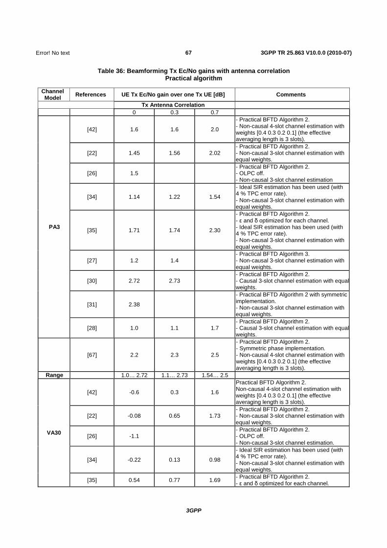
67
3GPP
Error! No text of specified
3GPP TR 25.863 V10.0.0 (2010-07)
Table 36: Beamforming Tx Ec/No gains with antenna correlation Practical algorithm
Channel Model References UE Tx Ec/No gain over one Tx UE [dB] Comments
Tx Antenna Correlation 0 0.3 0.7
PA3
[42] 1.6 1.6 2.0
- Practical BFTD Algorithm 2. - Non-causal 4-slot channel estimation with weights [0.4 0.3 0.2 0.1] (the effective averaging length is 3 slots).
[22] 1.45 1.56 2.02 - Practical BFTD Algorithm 2. - Non-causal 3-slot channel estimation with equal weights.
[26] 1.5 - Practical BFTD Algorithm 2. - OLPC off. - Non-causal 3-slot channel estimation
[34] 1.14 1.22 1.54
- Ideal SIR estimation has been used (with 4 % TPC error rate). - Non-causal 3-slot channel estimation with equal weights.
[35] 1.71 1.74 2.30
- Practical BFTD Algorithm 2. - ε and δ optimized for each channel. - Ideal SIR estimation has been used (with 4 % TPC error rate). - Non-causal 3-slot channel estimation with equal weights.
[27] 1.2 1.4 - Practical BFTD Algorithm 3. - Non-causal 3-slot channel estimation with equal weights.
[30] 2.72 2.73 - Practical BFTD Algorithm 2. - Causal 3-slot channel estimation with equal weights.
[31] 2.38
- Practical BFTD Algorithm 2 with symmetric implementation. - Non-causal 3-slot channel estimation with equal weights.
[28] 1.0 1.1 1.7 - Practical BFTD Algorithm 2. - Causal 3-slot channel estimation with equal weights.
[67] 2.2 2.3 2.5
- Practical BFTD Algorithm 2. - Symmetric phase implementation. - Non-causal 4-slot channel estimation with weights [0.4 0.3 0.2 0.1] (the effective averaging length is 3 slots).
Range 1.0… 2.72 1.1… 2.73 1.54… 2.5
VA30
[42] -0.6 0.3 1.6
Practical BFTD Algorithm 2. Non-causal 4-slot channel estimation with weights [0.4 0.3 0.2 0.1] (the effective averaging length is 3 slots).
[22] -0.08 0.65 1.73 - Practical BFTD Algorithm 2. - Non-causal 3-slot channel estimation with equal weights.
[26] -1.1 - Practical BFTD Algorithm 2. - OLPC off. - Non-causal 3-slot channel estimation.
[34] -0.22 0.13 0.98
- Ideal SIR estimation has been used (with 4 % TPC error rate). - Non-causal 3-slot channel estimation with equal weights.
[35] 0.54 0.77 1.69 - Practical BFTD Algorithm 2. - ε and δ optimized for each channel.

68
3GPP
Error! No text of specified
3GPP TR 25.863 V10.0.0 (2010-07)
- Ideal SIR estimation has been used (with 4 % TPC error rate). - Non-causal 3-slot channel estimation with equal weights.
[27] -0.3 0.1 - Practical BFTD Algorithm 3. - Non-causal 3-slot channel estimation with equal weights.
[30] 0.04 1.86 - Practical BFTD Algorithm 2. - Causal 3-slot channel estimation with equal weights.
[31] -0.37
- Practical BFTD Algorithm 2 with symmetric implementation. - Non-causal 3-slot channel estimation with equal weights.
[28] -0.8 0.3 1.5 - Practical BFTD Algorithm 2. - Causal 3-slot channel estimation with equal weights.
[67] -0.2 0.8 2.0
- Practical BFTD Algorithm 2. - Symmetric phase implementation - Non-causal 4-slot channel estimation with weights [0.4 0.3 0.2 0.1] (the effective averaging length is 3 slots).
Range -0.8… 0.54 0.1… 1.86 0.98… 2.0
Table 37 contains the simulation results for practical beamforming algorithms 2 and 4 defined in section 4.3.2 with Tx and Rx correlations = 0.3.
Table 37: Beamforming Rx Ec/No gains with Tx and Rx antenna correlation Practical algorithm
Channel Model References Node B Rx Ec/No gain over one Tx UE [dB] Comments
Tx and Rx Antenna Correlation = 0.3
PA3
[30] 2.94 - Practical BFTD Algorithm 2. - Causal 3-slot channel estimation with equal weights.
[31] 2.77
- Practical BFTD Algorithm 2 with symmetric implementation. - Non-causal 3-slot channel estimation with equal weights.
Range 2.77… 2.94
VA30
[30] 1.89 - Practical BFTD Algorithm 2. - Causal 3-slot channel estimation with equal weights.
[31] 2.15
- Practical BFTD Algorithm 2 with symmetric implementation. - Non-causal 3-slot channel estimation with equal weights.
Range 1.89 ... 2.15
6.2.2.1 Results for a Practical Node-B
The impact of uplink beamforming transmit diversity (BF) on a practical NodeB receiver is assessed using Practical BFTD Algorithm 1 described in section 4.3.2. It is assumed that the UE applies a given practical BF algorithm independently of NodeB (i.e. without informing NodeB) and there are no modifications of practical NodeB receiver algorithms.
The simulation assumptions used for Open Loop (OL) beamforming antenna transmit diversity are a subset of the assumptions in section 5.1. This simulation was conducted using 2 ms TTI with a TBS of 2020 without outer loop power

69
3GPP
Error! No text of specified
3GPP TR 25.863 V10.0.0 (2010-07)
control. Additionally, the antenna imbalance was assumed to be 0 dB and the Tx and Rx antenna correlations were assumed to be 0. UE DTX was also turned off.
The relative Rx Ec/No gain values for different channel propagation environments are tabulated in table 37a.
Table 37a: Link-level Simulation Results for Practical BFTD Algorithm 1
Antenna Correlation
(Tx, Rx)
Rx Ec/No Gain[dB]
PA3 VA30 VA120
(0, 0) -2.6 -1.4 -1.4
6.2.3 HS-DPCCH Performance in Soft Handover with Beamforming Transmit Diversity
6.2.3.1 Notation
In this contribution, the following variables are used.
GTx1->A: The antenna gain for the link from Antenna 1 (Tx1) to A which is the serving NodeB.
GTx2->A: The antenna gain for the link from Antenna 2 (Tx2) to A which is the serving NodeB.
GTx1->B: The antenna gain for the link from Antenna 1 (Tx1) to B which is the non-serving NodeB.
GTx2->B: The antenna gain for the link from Antenna 2 (Tx2) to B which is the non-serving NodeB.
IA->B: The imbalance between the two links from UE Antenna 1 to A and from UE Antenna 1 to B where A and B are the two NodeB's in the active set. The UE is in soft handover. In other words IA->B = GTx1-
>A- GTx1->B.

70
3GPP
Error! No text of specified
3GPP TR 25.863 V10.0.0 (2010-07)
These variables along with the simulation framework are shown in figure 28.
Figure 28: Simulation framework where the UE is in soft handover with Serving NodeB A and Non-Serving NodeB B
The imbalance between the antennas (Tx1 and Tx2) is different for the links to the serving and non-serving NodeB's. They are indicated below:
IUE->A = GTx1->A - GTx2->A: The imbalance between the two transmit antennas Tx1 and Tx2 for the radio link to the serving NodeB A.
IUE->B = GTx1->B - GTx2->B: The imbalance between the two transmit antennas Tx1 and Tx2 for the radio link to the non-serving NodeB B.
In this simulation, it is assumed that the path loss to the serving and non-serving NodeB cells are the same i.e. IA->B = GTx1->A- GTx1->B = 0 dB which can be considered as a worst case scenario and rather unlikely. The beamforming algorithm operates on the combined TPC command that is finally applied to the UE transmit power.

71
3GPP
Error! No text of specified
3GPP TR 25.863 V10.0.0 (2010-07)
6.2.3.2 HS-DPCCH Performance
Table 37b shows the HS-DPCCH ACK/NACK Miss detection and Decoding error rate performance when BFTD is applied at the UE.
Table 37b: HS-DPCCH ACK/NACK performance due to Beamforming in SHO
Beamforming HS-DPCCH ACK/NACK miss detection and decoding error rate [%]@ C/P=4 dB (Baseline value, Beamforming value)
SHO Link Imbalance
IA->B = 0 dB
Serving Cell Imbalance IUE->A IUE->A = 0 dB
Non Serving Cell Imbalance IUE->B IUE->B = 0 dB IUE->B = 3 dB IUE->B = -3 dB
PA3 (0.8 %, 1.5 %)† (0.8 %, 2.8 %) (0.8 %, 0.09 %) VA30 (0.02 %, 0.04 %) (0.02 %, 0.2 %) (0.02 %, 0.02 %) † The data format in the table is (Baseline value, BFTD value).
Table 37c shows the HS-DPCCH CQI Decoding error rate performance when Beamforming is applied at the UE. In this simulation framework, the UE is in soft handover with two cells in the active set.
Table 37c: HS-DPCCH CQI performance loss due to Beamforming in SHO
Beamforming HS-DPCCH CQI decoding error rate [%]@ C/P=0 dB (Baseline value, Beamforming value)
SHO Link Imbalance
IA->B = 0 dB.
Serving Cell Imbalance IUE->A IUE->A = 0 dB
Non Serving Cell Imbalance IUE->B IUE->B = 0 dB IUE->B = 3 dB IUE->B = -3 dB
PA3 (1 %, 1.5 %)† (1 %, 3.1 %) (1 %, 0.9 %) VA30 (0.06 %, 0.07 %) (0.06 %, 0.37 %) (0.06 %, 0.04 %) † The data format in the table is (Baseline value, BFTD value).
Table 38a shows the HS-DPCCH power offset required to achieve 1 % BER on the ACK/NACK when BTFD is applied by the UE.
Table 38a: HS-DPCCH ACK/NACK performance due to Beamforming in SHO
Beamforming HS-DPCCH ACK/NACK miss detection and decoding error rate [%]@ C/P=4 dB (Baseline value, Beamforming value)
SHO Link Imbalance
IA->B = 0 dB
Serving Cell Imbalance IUE->A IUE->A = 0 dB
Non Serving Cell Imbalance IUE->B IUE->B = 0 dB IUE->B = 3 dB IUE->B = -3 dB
PA3 (3.2, 5.6)† (3.2, 7.6) (3.2, 3.7) VA30 (-1.15, -0.76) (-1.15, 1.2) (-1.15, -1.87) † The data format in the table is (Baseline value, BFTD value).

72
3GPP
Error! No text of specified
3GPP TR 25.863 V10.0.0 (2010-07)
Table 38b shows the HS-DPCCH offset required to obtain 1 % BLER on the CQI when Beamforming is applied at the UE. In this simulation framework, the UE is in soft handover with two cells in the active set.
Table 38b: HS-DPCCH CQI performance loss due to Beamforming in SHO
Beamforming HS-DPCCH CQI decoding error rate [%]@ C/P=0 dB (Baseline value, Beamforming value)
SHO Link Imbalance
IA->B = 0 dB.
Serving Cell Imbalance IUE->A IUE->A = 0 dB
Non Serving Cell Imbalance IUE->B IUE->B = 0 dB IUE->B = 3 dB IUE->B = -3 dB
PA3 (0.26, 2.1)† (0.26, 4.7) (0.26, -0.16) VA30 (-4.2, -4.06) (-4.2, -1.8) (-4.2, -5.01) † The data format in the table is (Baseline value, BFTD value).
In a real system, SHO may include more radio links and link imbalances of a few dB may be encountered, and the probability of radio links with 0 dB imbalance is very low. The HS-DPCCH impact due to BFTD for UEs in SHO conditions with > 0 dB radio link imbalance could be much smaller than what tables 37a, 37b, 38a and 38b implies.
6.3 Uplink Transmit Diversity Link Level Simulations with Discontinuous Transmission
6.3.1 Discontinuous transmission description Voice over IP service of 160 kbps was simulated for practical switched antenna and beamforming transmit diversity schemes. One data packet was generated every 16 ms. DPCCH transmission precedes data transmission on E-DPDCH by 2 slots and follows it by 1 slot totalling 4 ms (6 slots) of DPCCH transmission every 16 ms.
6.3.2 Link level simulation results Gain due to DTX columns in the following tables compare the Tx diversity gains achieved in the presence of DTX with the gains achieved in the absence of DTX (negative value indicates less improvement when discontinuous transmission is present).
Table 38: Tx and Rx Ec/No gains - Practical Switched Antenn Diversity scheme, no antenna correlation, no antenna imbalance [33]
Channel Gain over Ref "Gain" due to DTX Rx Ec/No Tx Ec/No Rx Ec/No Tx Ec/No
PA3 -0.50 0.92 0.30 0.14 VA3 -0.30 0.30 0.00 0.01 VA30 -0.10 -0.01 0.20 0.10
Table 39: Tx and Rx Ec/No gains - Practical Beamforming scheme, no antenna correlation, no antenna imbalance [33]
Channel Gain over Ref "Gain" due to DTX Rx Ec/No Tx Ec/No Rx Ec/No Tx Ec/No
PA3 -0.45 0.88 -0.05 -0.38 VA3 -0.20 0.26 0.00 -0.22 VA30 -0.10 -0.10 -0.10 -0.06

73
3GPP
Error! No text of specified
3GPP TR 25.863 V10.0.0 (2010-07)
6.4 Uplink Transmit Diversity Link Level Simulations with Soft Handover
6.4.1 Soft Handover Simulations Description This section presents some link level results including soft handover to illustrate SHO impact due to ULTD. Two scenarios are considered:
- 2 way soft handover with equal link power; and
- 2 way SHO with 2dB imbalance.
In a real system SHO may include more radio links and link imbalances of a few dB may be encountered, and the probability of radio links with 0 dB imbalance is very low. The SHO impact for UEs with > 2 dB radio link imbalance could be much smaller than what tables 39a and 39b imply.
An antenna imbalance of 0 dB is assumed, and 0 % correlation. Other simulation results align with section 5.1.
6.4.2 Link Level Simulations Results This section presents terminal TX power gains and RX Ec/N0 power gains (positive value indicates smaller Ec/N0 compared to reference) obtained with the practical algorithms. The reference case is a single TX antenna setup in soft handover. Results for radio links imbalance 0, -2 dB are performed with Tx antenna imbalance 0 dB and correlation 0 %.
Table 39a: UE mean Tx power gains [dB] v/s radio link imbalance
Open Loop Beamforming Open Loop ASD Radio links imbalance PA3 VA3 VA30 PA3 VA3 VA30
0 dB 0.683 0.167 -0.292 0.384 0.127 -0.05 - 2dB 0.8 0.27 -0.29 0.49 0.17 -0.09
Table 39b: NodeB mean RX Ec/No gains [dB] v/s radio link imbalance
Open Loop Beamforming Open Loop ASD Radio links imbalance PA3 VA3 VA30 PA3 VA3 VA30
0 dB -0.3 -0.3 -0.33 -0.2 -0.1 -0.07 - 2dB -0.4 -0.34 -0.38 -0.2 -0.16 -0.12
6.5 Uplink Transmit Diversity Link Level Simulations with Incorrect TPC command delay
The results presented in this section correspond to the Practical BFTD algorithm 2 described in section 4.3 and to practical SATD algorithm described in section 4.3.1. The simulation assumptions used are a subset of assumptions in section 5.1 (simulation assumptions of higher priority). The simulations were conducted using 2ms TTI with a TBS of 2020. Additionally, the antenna imbalance was assumed to be 0 dB and UE DTX and Soft Handover were turned off. The e and d for the Practical BFTD algorithm 2 were assumed to be 12o and 25o respectively.
In table 39c, set of link level results is presented to assess the impact of the UE assuming an incorrect TPC command delay. This assumption is especially important for the beamforming algorithm which was described in section 4.3, which is a scheme that measures the link quality (as indicated by TPC commands from the Node B) after each adjustment of the antenna weights. For the loop to operate correctly, it is necessary that the association between the weight adjustment timing and the TPC feedback is correct.

74
3GPP
Error! No text of specified
3GPP TR 25.863 V10.0.0 (2010-07)
Simulations results in other sections of this report were generated under the assumption that the TPC delay is known to the terminal. However, the TPC command delay, and more generally, the power control behaviour in the Node B is not mandated by the specifications. Thus, the delay, among other parameters, is vendor and deployment specific, including dependency on propagation delay or cell size, or conceivably even on hardware loading.
Table 39c: Tx and Rx Ec/No gains - Practical uplink transmit diversity schemes, no antenna imbalance with incorrect TPC command delay assumption at the UE
Tx Antenna Correlation Open Loop Beamforming Open Loop ASD PA3 VA3 VA30 PA3 VA3 VA30
UE Tx power gains [dB] 0 % -3.26 -1.67 -0.99 0.94 0.42 -0.04
Node B Rx Ec/N0 gains [dB] 0 % -2.15 -1.04 -1.05 -0.20 -0.09 -0.12
NOTE: A positive Tx power gain means less Tx power, and a positive Rx Ec/N0 gain means smaller Rx Ec/N0, compared to the reference single Tx antenna configuration.
6.6 Uplink Transmit Diversity Link Level Simulations with Multipath Propagation
The results presented in this section correspond to the Practical BFTD algorithm 2 described in section 4.3.2 and to practical SATD algorithm described in section 4.3.1. The simulation assumptions used are a subset of assumptions in section 5.1 (simulation assumptions of higher priority). The simulations were conducted using 2 ms TTI with a TBS of 2020. Additionally, the antenna imbalance was assumed to be 0 dB and UE DTX and Soft Handover were turned off. The e and d for the Practical BFTD algorithm 2 were assumed to be 12o and 25o respectively.
Table 39d shows the Tx diversity gains obtained for different Tx antenna correlation and under a range of propagation conditions.
Table 39d: Tx and Rx Ec/No gains - Practical uplink transmit diversity schemes, no antenna imbalance under different propagation conditions
Tx Antenna Correlation Open Loop Beamforming Open Loop ASD PA3 VA3 VA30 PA3 VA3 VA30
UE Tx power gains [dB] 0 % 1.71 0.54 0.04 1.03 0.38 -0.02 30 % 1.74 0.77 0.29 1.21 0.34 -0.05 70 % 2.30 1.69 1.32 0.76 0.24 0.01
Node B Rx Ec/N0 gains [dB] 0 % -0.30 -0.29 -0.05 -0.40 -0.20 -0.08 30 % -0.40 -0.20 0.05 -0.30 -0.10 -0.11 70 % -0.30 -0.20 0.24 -0.20 -0.10 0.02
NOTE: A positive Tx power gain means less Tx power, and a positive Rx Ec/N0 gain means smaller Rx Ec/N0, compared to the reference single Tx antenna configuration.
6.7 Conclusion on Link Evaluation Results
6.7.1 Switched Antenna Transmit Diversity The simulation results with practically implementable algorithms on switched antenna transmit diversity for balanced and uncorrelated antennae show that in PedA 3 km/h channel, a reduction (gain) up to 1.42 dB in the UE uplink transmit power can be achieved. In VehA 30 km/h channel, UE transmit power more similar to that of the single antenna case can be
75
3GPP
Error! No text of specified
3GPP TR 25.863 V10.0.0 (2010-07)
observed, difference ranging from 0.15 dB loss to 0.2 dB gain. For more stringent BLER targets compared to the reference (1 % residual BLER after 4th transmission) worse performance - smaller UE Tx power gains or larger losses - are observed.
In the presence of antenna correlation (balanced antennae), the Tx power gains in PedA 3 km/h channel are somewhat smaller than in case of no antenna correlation. Similarly the loss observed in VehA 30 km/h channel is somewhat reduced.
In the presence of antenna imbalance (uncorrelated antennae), for both studied channels (PedA 3 km/h and VehA 30 km/h), when the secondary antenna has lower gain than the primary (reference) antenna, up to 1.25 dB increase (loss) in UE Tx power is observed. When the secondary antenna has higher gain than the primary (reference) antenna, reductions (gain) up to 2.06 dB to 3.2 dB in UE Tx powers is seen.
In all simulated cases (PedA 3 km/h and VehA 30 km/h channels for uncorrelated and balanced, uncorrelated and imbalanced, and correlated and balanced antennae), no gains were observed, but typically an increase (loss) up to 0.73 dB is observed for the Node B Rx Ec/No. For more stringent BLER targets compared to the reference (1 % residual BLER after 4th transmission) an increased loss in Node B Rx Ec/No is observed.
When the maximum switching frequency is reduced from 100 Hz to 50 Hz or 25 Hz, an overall reduction in the UE Tx power performance is seen - gains decrease or loss increase. Typically, but not consistently a somewhat smaller loss is observed in the Node B Rx Ec/No.
6.7.2 Beamforming Transmit Diversity The simulation results with practically implementable algorithms on beamforming antenna transmit diversity for balanced and uncorrelated antennae show that in PedA 3 km/h channel, a reduction (gain) in the range of 1.0 dB to 2.77 dB in the UE uplink transmit power can be achieved. In VehA 30 km/h channel, UE transmit powers range from 1.46 dB loss to 0.54 dB gain relative to the single antenna case.
In the presence of antenna correlation (balanced antennae), the Tx power gains in PedA 3 km/h channel increase slightly and VehA 30 km/h channel shows UE transmit powers ranging from 0.8 dB loss to 2.15 dB gain.
In the presence of antenna imbalance (uncorrelated antennae), when the secondary antenna has lower gain than the primary (reference) antenna, for PedA 3 km/h Tx power performance ranging from 1.26 dB loss to 1.27 dB gain is observed. For VehA 30 km/h all simulated cases indicate loss from 0.83 dB to 2.2 dB. When the secondary antenna has higher gain than the primary (reference) antenna, significant gains up to 4.24 dB are observed for PedA 3 km/h channel. For VehA 30 km/h channel a range from small loss to 2.2 dB gain in UE Tx power is seen.
In all simulated cases (PedA 3 km/h and VehA 30 km/h channels for uncorrelated and balanced, uncorrelated and imbalanced, and correlated and balanced antennae) an increase (loss) typically in the range of 0.1 to 0.5 dB is observed for the Node B Rx Ec/No although in some cases loss up to 2.1 dB and gain up to 0.23 dB is seen.

76
3GPP
Error! No text of specified
3GPP TR 25.863 V10.0.0 (2010-07)
7 System Evaluation Results This section summarizes the system level evaluations for switched and beamforming antenna diversity. The results for switched antenna diversity are presented in section 7.1 while the results for beamforming diversity are presented in section 7.2. Unless otherwise is stated the results are based on the system simulation parameters previously described in section 5.3.2.
7.1 Switched Antenna Transmit Diversity
7.1.1 Full Buffer Traffic
7.1.1.1 Results for inter-site distance 1km
7.1.1.1.1 Results for 0 dB long-term antenna imbalance and 2D antennas
Table 40 presents the average user data rates, the 10th percentile user data rates and the average transmit power for the different user densities that was studied for a PA3 channel when the inter-site distance is 1 km. Both absolute and relative numbers are presented. All relative numbers are presented with respect to baseline case (without transmit diversity).

77
3GPP
Error! No text of specified
3GPP TR 25.863 V10.0.0 (2010-07)
Table 40: Average user data rates, 10th percentile user data rates and average transmit power for the studied user densities in a PA3 channel when the inter-site distance is 1 km
Average data rates Reference Algorithms Average number of users per cell Comments 0.25 0.5 1 2 4 10
[53] Baseline [kbps] 1 582 1 455 1 173 788 417 154
Genie [kbps] 1 590 1 512 1 294 916 517 198 Practical [kbps] 1 608 1 495 1 23 844 453 168
Gain with Genie [%] 0.5 3.9 10.3 16.2 24.0 28.5
Gain with Practical [%] 1.6 2.7 4.3 7.1 8.6 9.1
[44] Baseline [kbps] 1 233.7 1 235.5 1 230.9 498.7 135.7
Genie [kbps] Practical [kbps] 1 270.2 1 271.9 1 267.5 539.8 146.3
Gain with Genie [%]
Gain with Practical [%] 2.96 2.96 2.98 8.24 7.85
[63] Baseline [kbps] 1 312 803 410 145 Note 1
Genie [kbps] 1 450 908 480 175 Practical [kbps] 1 369 838 434 155
Gain with Genie [%] 10.5 13 17 21
Gain with Practical [%] 4 4 6 7
[61] Baseline [kbps] 2 114 1 864 1 787 942 395
Genie [kbps] 2 162 1 944 1 986 1 127 471 Practical [kbps] 2 125 1 895 1 870 1 022 426
Gain with Genie [%] 2.36 4.48 11.11 19.54 19.41
Gain with Practical [%] 0.56 1.70 4.58 8.38 7.83
[57] Baseline [kbps] 2 124.8 1 608.1 1 101.8 621.0 272.0 Note 1
Genie [kbps] Practical
[kbps] 2 148.8 1 639.7 1 127.0 630.4 284.5
Gain with Genie [%]
Gain with Practical [%] 1.13 1.96 2.29 1.52 4.60

78
3GPP
Error! No text of specified
3GPP TR 25.863 V10.0.0 (2010-07)
10th percentile user data rates Reference Algorithms Average number of users per cell Comments
0.25 0.5 1 2 4 10 [53] Baseline
[kbps] 1 470 1 023 423 174 138 68
Genie [kbps] 1 531 1 200 599 256 197 93 Practical [kbps] 1 525 1 055 465 199 149 75
Gain with Genie [%] 4.1 17.3 41.6 47.1 42.8 36.8
Gain with Practical [%] 3.7 3.1 9..9 14.4 8 10.3
[44] Baseline [kbps] 1 206.1 1 206.5 1 208.1 314.9 100.8
Genie [kbps] Practical [kbps] 1 238.5 1 239.4 1 241.4 336.4 108.2
Gain with Genie [%]
Gain with Practical [%] 2.69 2.73 2.76 6.84 7.38
[63] Baseline [kbps] 543 326 190 74 Note 1
Genie [kbps] 672 368 229 92 Practical [kbps] 593 319 198 77
Gain with Genie [%] 24 18 20 24
Gain with Practical [%] 9 -2 4 4
[61] Baseline [kbps] 1 720 1 193 1 173 473 261
Genie [kbps] 1 762 1 273 1 498 708 348 Practical [kbps] 1 745 1 251 1 324 537 287
Gain with Genie [kbps] 2.44 6.71 27.71 49.68 33.33
Gain with Practical [kbps]
1.45 4.86 12.87 13.53 9.96
[57] Baseline [kbps] 978.4 488.9 244.0 52.3 50.6 Note 1
Genie [kbps] Practical
[kbps] 957.7 504.9 255.3 59.8 50.8
Gain with Genie [kbps]
Gain with Practical [kbps]
-2.12 % 3.28 % 4.64 % 14.36 % 0.44 %

79
3GPP
Error! No text of specified
3GPP TR 25.863 V10.0.0 (2010-07)
Average transmit power Reference Algorithms Average number of users per cell Comments
0.25 0.5 1 2 4 10 [53] Baseline
[dBm] 5.93 6.60 6.71 6.18 4.65 1.30
Gain with Genie [dB] 1.25 1.83 1.82 1.38 1.12 0.52
Gain with Practical[dB] 1.1 0.95 1.15 0.91 0.96 0.93
[44] Baseline [dBm] -18.48 -18.39 -17.52 -11.99 -10.41 Note 2
Gain with Genie [dB]
Gain with Practical[dB] 1.62 1.67 1.8 1.54 1.29
[63] Baseline [dBm] 13.00 11.13 9.03 6.04 Note 1
Gain with Genie [dB] 0.84 0.47 0.35 0.30
Gain with Practical [dB] 0.32 0.00 -0.10 -0.15
[61] Baseline [dBm] 2.17 2.18 1.77 0.37 -2.38
Gain with Genie [dB] 1.69 1.70 1.62 1.03 1.22
Gain with Practical [dB] 1.01 1.01 0.97 0.66 0.70
[57] Baseline [dBm] 0.49 0.16 -1.77 -5.24 -6.02 Note 1
Gain with Genie [dB]
Gain with Practical [dB] 0.69 0.55 0.84 0.77 0.91
NOTE 1: Ideal SIR estimation has been assumed when generating the TPC commands. NOTE 2: Here the average transmit power refers to the DPCCH power.
Table 41 presents the average user data rates, the 10th percentile user data rates and the average transmit power for the studied user densities in a VA30 channel when the inter-site distance is 1 km. Both absolute and relative numbers are presented. The relative numbers are presented with respect to the baseline case (without transmit diversity).

80
3GPP
Error! No text of specified
3GPP TR 25.863 V10.0.0 (2010-07)
Table 41: Average user data rates (in kbps), 10th percentile user data rates and average transmit power for the studied user densities in a VA30 channel when the inter-site distance is 1 km
Average data rates Reference Algorithms Average number of users per cell Comments
0.25 0.5 1 2 4 10 [53] Baseline [kbps] 1 583 1 380 1 077 713 393 150
Genie [kbps] 1 593 1 398 1 133 765 416 159 Practical [kbps] 1 581 1 361 1 072 715 394 148 Gain with Genie [%] 0.6 1.3 5.2 7.3 5.9 6.0 Gain with Practical [%] -0.1 -1.4 -0.5 0.2 0.3 -1.3
[44] Baseline [kbps] 1 327.2 1 329.2 1 317.9 475.4 127.3 Genie [kbps] Practical [kbps] 1 347.8 1 350.1 1 336.3 477.1 129 Gain with Genie [%] Gain with Practical [%] 1.56 1.57 1.4 0.36 1.28
[63] Baseline [kbps] 1 091 685 371 140 Note 1 Genie [kbps] 1 132 709 385 140 Practical [kbps] 1 114 695 378 137 Gain with Genie [%] 3.75 3.5 3.8 0 Gain with Practical [%] 2.1 1.5 1.9 -2
[61] Baseline [kbps] 1 837 1 565 1 528 774 324 Genie [kbps] 1 857 1 592 1 578 810 338 Practical [kbps] 1 836 1 571 1 542 788 329 Gain with Genie [%] 1.09 1.73 3.27 4.65 4.32 Gain with Practical [%] -0.05 0.38 0.92 1.81 1.54
[57] Baseline [kbps] 1 766.8 1 394.1 1 004.1 624.0 316.5 Note 1 Genie [kbps] Practical [kbps] 1 792.2 1 400.7 1 014.7 627.7 322.6 Gain with Genie [%] Gain with Practical [%] 1.44 0.47 1.06 0.58 1.93
10th percentile user data rates Reference Algorithms Average number of users per cell Comments
0.25 0.5 1 2 4 10 [53] Baseline [kbps] 1 270 677 337 191 119 64
Genie [kbps] 1 310 735 422 228 124 72 Practical [kbps] 1 275 540 310 191 108 61 Gain with Genie [%] 3.2 8.6 25.2 19.4 4.2 11.8 Gain with Practical [%] 0.4 -20.2 -8 0 -9.2 -5.3
[44] Baseline [kbps] 1 312.5 1 310.7 1 305.9 249 95.9 Genie [kbps] Practical [kbps] 1 329.2 1 328.1 1 321 245.4 95.9 Gain with Genie [%] Gain with Practical [%] 1.27 1.33 1.16 -1.43 0
[63] Baseline [kbps] 482 285 166 65 Note 1 Genie [kbps] 516 290 181 71 Practical [kbps] 503 281 175 70 Gain with Genie [%] 7 1.75 9 9 Gain with Practical [%] 4.3 -1.4 5.4 7.7
[61] Baseline [kbps] 1 308 834 808 391 219 Genie [kbps] 1 324 861 885 436 236 Practical [kbps] 1 312 846 839 407 227 Gain with Genie [%] 1.22 3.24 9.53 11.51 7.76 Gain with Practical [%] 0.31 1.44 3.84 4.09 3.65
[57] Baseline [kbps] 729.0 470.0 190.5 61.7 50.6 Note 1 Genie [kbps] Practical [kbps] 837.1 491.3 231.7 71.7 50.7 Gain with Genie [%] Gain with Practical [%] 14.83 4.54 21.59 16.34 0.18
Average transmit power Reference Algorithms Average number of users per cell Comments

81
3GPP
Error! No text of specified
3GPP TR 25.863 V10.0.0 (2010-07)
0.25 0.5 1 2 4 10 [53] Baseline [dBm] 5.71 6.70 7.21 6.53 4.79 0.48
Gain with Genie [dB] 1.15 0.62 0.66 1.04 0.46 0.23 Gain with Practical [dB] 0.4 0.48 0.26 0.50 0.28 0.16
[44] Baseline [dBm] -18.6 -18.44 -17.5 -12.89 -11.14 Note 2 Gain with Genie [dB] Gain with Practical [dB] 0.38 0.39 0.4 0.31 0.46
[63] Baseline [dBm] 13.06 11.21 8.85 5.56 Note 1 Gain with Genie [dB] 0.21 0.22 -0.26 0.08 Gain with Practical [dB] 0.27 0.31 -0.17 0.19
[61] Baseline [dBm] 3.04 2.60 2.19 0.19 -2.67 Gain with Genie [dB] 0.75 0.73 0.67 0.59 0.63 Gain with Practical [dB] 0.50 0.49 0.46 0.40 0.43
[57] Baseline [dBm] 1.33 -0.60 -2.28 -4.31 -7.46 Note 1 Gain with Genie [dB] Gain with Practical [dB] 0.43 0.48 0.38 0.49 0.49
NOTE 1: Ideal SIR estimation has been assumed when generating the TPC commands. NOTE 2: Here the average transmit power refers to the DPCCH power.
Table 42 presents the average user data rates, the 10th percentile user data rates and the average transmit power for the studied user densities in a PA0.1 channel when the inter-site distance is 1 km. Both absolute and relative numbers are presented. In the case relative numbers are presented they are with respect to baseline case without antenna switching diversity.
Table 42: Average user data rates, 10th percentile user data rates and average transmit power for the studied user densities in a PA 0.1 channel when the inter-site distance is 1 km
Average data rates Reference Algorithms Average number of users per cell Comments
0.25 0.5 1 2 4 10 [44] Baseline [kbps] 1 200.4 1 201.8 1 198.4 544 144.9
Genie [kbps] Practical [kbps] 1247 1249 1246.3 609.4 165.1 Gain with Genie [%] Gain with Practical [%] 3.88 3.93 4 12.03 13.9
10th percentile user data rates Reference Algorithms Average number of users per cell Comments
0.25 0.5 1 2 4 10 [44] Baseline [kbps] 1 194.9 1 195.6 1 194.2 328.5 97.3
Genie [kbps] Practical [kbps] 1230.2 1231 1232.1 384.4 118.7 Gain with Genie [%] Gain with Practical [%] 2.95 2.96 3.17 17.01 21.97
Average transmit power Reference Algorithms Average number of users per cell Comments
0.25 0.5 1 2 4 10 [44] Baseline [dBm] -18.79 -18.75 -18.01 -12.58 -10.59 Note
Gain with Genie [dB] Gain with Practical [dB] 2.36 2.45 2.6 2.22 1.84
NOTE: Here the average transmit power refers to the DPCCH power.

82
3GPP
Error! No text of specified
3GPP TR 25.863 V10.0.0 (2010-07)
7.1.1.1.2 Results for 0 dB long-term antenna imbalance and 3D antenna
Table 43 present the average data rates, the 10th percentile user data rates and the average transmit power for the studied user densities in a PA3 channel when 3D antennas at the Node-B is modelled.
Table 43: Average data rates, 10th percentile user data rates and average transmit power for the studied user densities in a PA3 channel when 3D antennas at the Node-B are modelled
Average data rates Reference Algorithms Average number of users per cell Comments
0.25 0.5 1 2 4 10 [55] Baseline [kbps] 1 589 1 501 1 291 929 537 213
Genie [kbps] 1 602 1 536 1 373 1 017 606 244 Practical [kbps] 1 615 1 528 1 338 969 563 221 Gain with Genie [%] 0.8 2.3 6.4 9.5 12.8 14.5
Gain with Practical [%] 1.6 1.8 3.6 4.3 4.8 3.8
10th percentile user data rates Reference Algorithms Average number of users per cell Comments
0.25 0.5 1 2 4 10 [55] Baseline [kbps] 1 551 1 215 667 284 184 113
Genie [kbps] 1 572 1 318 829 366 243 130 Practical [kbps] 1 582 1 169 734 299 196 113 Gain with Genie [%] 1.3 8.4 24.3 28.8 32.1 15.0
Gain with Practical [%] 2 -3.8 10.0 5.1 6..5 0.2
Average transmit power Reference Algorithms Average number of users per cell Comments
0.25 0.5 1 2 4 10 [55] Baseline [dBm] 11.6 11.1 11.6 11.1 10.1 7.92
Gain with Genie [dB] 1.67 1.58 1.53 1.31 1.11 1.28
Gain with Practical [dB] 0.89 0.79 0.90 0.81 0.77 0.95

83
3GPP
Error! No text of specified
3GPP TR 25.863 V10.0.0 (2010-07)
Table 44 present the average data rates, the 10th percentile user data rates and the average transmit power for the studied user densities in a VA30 channel when 3D antennas at the Node-B are modelled.
Table 44: Average data rates, 10th percentile user data rates and average transmit power for the studied user densities in a VA30 channel when 3D antennas at the Node-B are modelled
Average data rates Reference Algorithms Average number of users per cell Comments
0.25 0.5 1 2 4 10 [55] Baseline [kbps] 1 594 1 458 1 240 866 499 200
Genie [kbps] 1 605 1 469 1 265 892 512 203 Practical [kbps] 1 591 1 460 1 232 867 496 196 Gain with Genie [%] 0.7 0.7 2 3 2.6 1.5 Gain with Practical [%] -0.2 0.1 -0.7 0.1 -0.6 -2.0
10th percentile user data rates Reference Algorithms Average number of users per cell Comments
0.25 0.5 1 2 4 10 [55] Baseline [kbps] 1 323 913 550 276 179 106
Genie [kbps] 1 352 912 565 309 191 106 Practical [kbps] 1 239 868 535 292 176 99 Gain with Genie [%] 2.2 -0.1 2.7 11.9 6.7 -0.3 Gain with Practical [%] -6.4 -4.9 -2.7 5.8 -1.7 -6.4
Average transmit power Reference Algorithms Average number of users per cell Comments
0.25 0.5 1 2 4 10 [55] Baseline [dBm] 10.6 12.2 12.2 11.0 9.72 7.15
Gain with Genie [dB] 0.86 0.66 0.75 0.65 0.47 0.48
Gain with Practical [dB] 0.35 0.25 0.38 0.48 0.26 0.37

84
3GPP
Error! No text of specified
3GPP TR 25.863 V10.0.0 (2010-07)
Table 44a present the average data rates, the 10th percentile user data rates and the average transmit power for the studied user densities in a VA120 channel when 3D antennas at the Node-B are modelled.
Table 44a: Average data rates, 10th percentile user data rates and average transmit power for the studied user densities in a VA120 channel when 3D antennas at the Node-B are modelled
Average data rates Reference Algorithms Average number of users per cell Comments
0.25 0.5 1 2 4 10 [79] Baseline [kbps] 1 574.8 1 267.7 940.4 570.7 263.0 46.3
Genie [kbps] 1 623.9 1 296.1 974.5 599.9 288.9 59.5 Practical [kbps] 1 596.6 1 261.5 944.9 576.5 269.8 54.7 Gain with Genie [%] 3.1 2.2 3.9 5.1 9.8 28.6 Gain with Practical [%]
1.3 -0.5 0.5 1.0 2.6 18.2
10th percentile user data rates Reference Algorithms Average number of users per cell Comments
0.25 0.5 1 2 4 10 [79] Baseline [kbps] 690.4 321.2 83.4 34.1 17.6 8.4
Genie [kbps] 721.3 285.0 86.1 43.4 30.9 12.6 Practical [kbps] 729.2 278.4 80.9 39.5 26.8 10.9 Gain with Genie [%] 4.5 -11.3 3.2 27.0 75.5 49.1 Gain with Practical [%]
5.6 -13.3 -2.9 15.8 52.1 29.7
Average transmit power Reference Algorithms Average number of users per cell Comments
0.25 0.5 1 2 4 10 [79] Baseline [dBm] 17.5 16.9 16.3 14.8 13.3 8.8
Gain with Genie [dB]
0.63 0.63 0.52 0.56 0.41 0.40
Gain with Practical [dB]
0.53 0.56 0.53 0.64 0.54 0.48

85
3GPP
Error! No text of specified
3GPP TR 25.863 V10.0.0 (2010-07)
7.1.1.1.3 Results for -4 dB long-term antenna imbalance and 2D antennas
Table 45 presents the average user data rates, 10th percentile user data rates and average transmit power for the studied user densities in a PA3 channel when the second antenna is associated with a long-term antenna imbalance of -4 dB.
Table 45: Average user data rates, 10th percentile user data rates and average transmit power for the studied user densities in a PA3 channel when the second antenna is associated
with a long term antenna imbalance of -4 dB
Average data rates Reference Algorithms Average number of users per cell Comments 0.25 0.5 1 2 4 10
[53] Baseline [kbps] 1 582 1 455 1 173 788 417 154 Genie [kbps] 1 578 1 514 1 284 889 485 - Practical [kbps] 1 580 1 497 1 227 803 416 - Gain with Genie [%]
-0.2 4 9.4 12.8 16.3 -
Gain with Practical [%]
-0.1 2.9 4.6 1.9 -0.3 -
[61] Baseline [kbps] 2 114 1 864 1 787 942 395 Genie [kbps] Practical [kbps] 2 084 1 827 1 735 898 367 Gain with Genie [%]
Gain with Practical [%] -1.39 -1.96 -2.99 -4.75 -6.90
[57] Baseline [kbps] 2 124.8 1 602.1 1 135.0 628.0 287.0 Note Genie [kbps] Practical [kbps] 2 130.9 1 608.2 1 157.5 622.1 289.9 Gain with Genie
[%]
Gain with Practical [%]
0.29 0.38 1.99 -0.94 1.01
10th percentile user data rates Reference Algorithms Average number of users per cell Comments
0.25 0.5 1 2 4 10 [53] Baseline [kbps] 1 470 1 023 423 174 138 68
Genie [kbps] 1 490 1 175 565 236 164 - Practical [kbps] 1 408 1 005 465 183 137 - Gain with Genie [%]
1.4 14.8 33.5 35.5 18.8 -
Gain with Practical [%]
4.2 -1.7 9.9 5.2 -0.7 -
[61] Baseline [kbps] 1727 1185 1182 457 261 Genie [kbps] Practical [kbps] 1 685 1 157 1 114 421 247 Gain with Genie [%]
Gain with Practical [%] -2.01 -2.98 -5.07 -10.97 -5.36
[57] Baseline [kbps] 978.4 470.8 249.0 52.1 50.6 Note Genie [kbps] Practical [kbps] 955.6 480.1 250.3 57.8 50.2 Gain with Genie
[%]
Gain with Practical [%]
-2.33 1.98 0.50 10.88 -0.82

86
3GPP
Error! No text of specified
3GPP TR 25.863 V10.0.0 (2010-07)
Average transmit power Reference Algorithms Average number of users per cell Comments
0.25 0.5 1 2 4 10 [53] Baseline [dBm] 5.93 6.60 6.71 6.18 4.65 1.30
Gain with Genie [dB]
-1 0.88 -0.11 -0.13 0.11 -
Gain with Practical [dB]
-1.72 -0.08 -0.72 -0.37 0.2 -
[61] Baseline [dBm] 2.17 2.18 1.77 0.37 -2.38 Gain with Genie [dB]
Gain with Practical [dB] -0.26 -0.21 -0.16 -0.13 -0.21
[57] Baseline [dBm] 0.49 -1.03 -2.99 -4.47 -6.52 Note Gain with Genie
[dB]
Gain with Practical [dB]
-0.56 -0.49 -0.47 -0.39 -0.18
NOTE: Ideal SIR estimation has been assumed when generating the TPC commands.

87
3GPP
Error! No text of specified
3GPP TR 25.863 V10.0.0 (2010-07)
Table 46 presents the average user data rates, 10th percentile user data rates and average transmit power for the studied user densities in a VA30 channel when the second antenna is associated with a long-term antenna imbalance of -4 dB.
Table 46: Average user data rates, 10th percentile user data rates and average transmit power for the studied user densities in a VA30 channel when the second antenna is associated
with a long term antenna imbalance of -4 dB
Average data rates Reference Algorithms Average number of users per cell Comments 0.25 0.5 1 2 4 10
[53] Baseline [kbps] 1 583 1 380 1 077 713 393 150 Genie [kbps] 1 575 1 386 1 101 723 397 146 Practical [kbps] 1 569 1 343 1 050 677 366 133 Gain with Genie [%] -0.5 0.5 2.2 1.4 1.0 -2.6
Gain with Practical [%] -0.9 -2.7 -2.5 -5.1 -6.8 -12.3
[57] Baseline [kbps] 1 785.0 1 405.1 1 019.4 624.2 315.5 Note Genie [kbps] Practical [kbps] 1 782.2 1 422.4 1 018.8 624.7 312.9 Gain with Genie
[%]
Gain with Practical [%] -0.15 1.23 -0.07 0.09 -0.83
10th percentile user data rates Reference Algorithms Average number of users per cell Comments
0.25 0.5 1 2 4 10 [53] Baseline [kbps] 1 270 677 337 191 120 64
Genie [kbps] 1 280 710 363 192 122 64 Practical [kbps] 1 240 605 339 169 101 56 Gain with Genie [%] 0.8 4.9 7.7 0.6 1.7 -0.3
Gain with Practical [%] -2.4 -10.6 0.6 -11.4 -15.4 -12.4
[57] Baseline [kbps] 781.3 448.2 230.8 70.8 50.3 Note Genie [kbps] Practical [kbps] 774.8 451.3 238.3 76.0 50.4 Gain with Genie
[%]
Gain with Practical [%] -0.83 0.68 3.27 7.26 0.18
Average transmit power Reference Algorithms Average number of users per cell Comments
0.25 0.5 1 2 4 10 [53] Baseline [dBm] 5.71 6.70 7.21 6.53 4.08 0.48
Gain with Genie [dB] -0.11 -0.59 -0.34 0.185 -0.12 -0.16
Gain with Practical [dB] -0.94 -1.24 -0.84 -0.24 -0.49 -0.28
[57] Baseline [dBm] 0.90 -0.32 -2.37 -4.55 -6.84 Note Gain with Genie
[dB]
Gain with Practical [dB] -0.64 -0.55 -0.50 -0.48 -0.41
NOTE: Ideal SIR estimation has been assumed when generating the TPC commands.
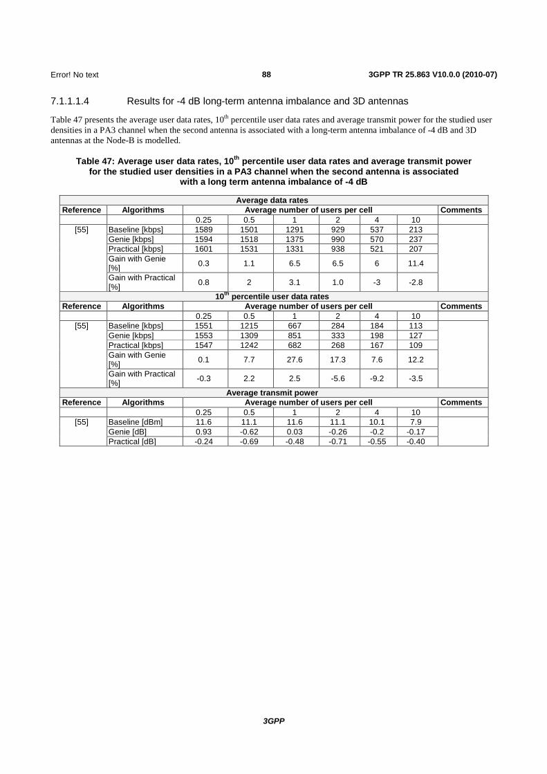
88
3GPP
Error! No text of specified
3GPP TR 25.863 V10.0.0 (2010-07)
7.1.1.1.4 Results for -4 dB long-term antenna imbalance and 3D antennas
Table 47 presents the average user data rates, 10th percentile user data rates and average transmit power for the studied user densities in a PA3 channel when the second antenna is associated with a long-term antenna imbalance of -4 dB and 3D antennas at the Node-B is modelled.
Table 47: Average user data rates, 10th percentile user data rates and average transmit power for the studied user densities in a PA3 channel when the second antenna is associated
with a long term antenna imbalance of -4 dB
Average data rates Reference Algorithms Average number of users per cell Comments 0.25 0.5 1 2 4 10
[55] Baseline [kbps] 1589 1501 1291 929 537 213 Genie [kbps] 1594 1518 1375 990 570 237 Practical [kbps] 1601 1531 1331 938 521 207 Gain with Genie [%] 0.3 1.1 6.5 6.5 6 11.4
Gain with Practical [%] 0.8 2 3.1 1.0 -3 -2.8
10th percentile user data rates Reference Algorithms Average number of users per cell Comments
0.25 0.5 1 2 4 10 [55] Baseline [kbps] 1551 1215 667 284 184 113
Genie [kbps] 1553 1309 851 333 198 127 Practical [kbps] 1547 1242 682 268 167 109 Gain with Genie [%] 0.1 7.7 27.6 17.3 7.6 12.2
Gain with Practical [%] -0.3 2.2 2.5 -5.6 -9.2 -3.5
Average transmit power Reference Algorithms Average number of users per cell Comments
0.25 0.5 1 2 4 10 [55] Baseline [dBm] 11.6 11.1 11.6 11.1 10.1 7.9
Genie [dB] 0.93 -0.62 0.03 -0.26 -0.2 -0.17 Practical [dB] -0.24 -0.69 -0.48 -0.71 -0.55 -0.40

89
3GPP
Error! No text of specified
3GPP TR 25.863 V10.0.0 (2010-07)
Table 48 presents the average user data rates, 10th percentile user data rates and average transmit power for the studied user densities in a VA30 channel when the second antenna is associated with a long-term antenna imbalance of -4 dB and 3D antennas at the Node-B is modelled.
Table 48: Average user data rates, 10th percentile user data rates and average transmit power for the studied user densities in a VA30 channel when the second antenna is associated
with a long term antenna imbalance of -4 dB
Average data rates Reference Algorithms Average number of users per cell Comments 0.25 0.5 1 2 4 10
[55] Baseline [kbps] 1 594 1 458 1 240 866 499 200 Genie [kbps] 1 624 1 515 1 269 885 511 206 Practical [kbps] 1 623 1 486 1 212 842 475 188 Gain with Genie [%] 1.8 3.9 2.3 2.2 2.4 3.0 Gain with practical [%] 1.8 1.9 -2.3 -2.7 -4.8 -6.0
10th percentile user data rates Reference Algorithms Average number of users per cell Comments
0.25 0.5 1 2 4 10 [55] Baseline [kbps] 1 323 913 550 277 179 106
Genie [kbps] 1 411 1 164 576 316 192 109 Practical [kbps] 1 356 973 482 285 171 107 Gain with Genie [%] 6.7 27.5 4.76 14.2 7.1 2.8 Gain with Practical [%] 2.4 6.6 -12.4 2.9 -4.5 1.0
Average transmit power Reference Algorithms Average number of users per cell Comments
0.25 0.5 1 2 4 10 [55] Baseline [dBm] 10.6 12.2 12.2 11.0 9.72 7.1
Gain with Genie [dB] -1.44 0.31 0.16 -0.37 -0.30 -0.12
Gain with Practical [dB] -1.58 0.04 -0.44 -0.85 -0.70 -0.50

90
3GPP
Error! No text of specified
3GPP TR 25.863 V10.0.0 (2010-07)
Table 48a1 presents the average user data rates, 10th percentile user data rates and average transmit power for the studied user densities in a VA120 channel when the second antenna is associated with a long-term antenna imbalance of -4 dB and 3D antennas at the Node-B is modelled.
Table 48a1: Average user data rates, 10th percentile user data rates and average transmit power for the studied user densities in a VA120 channel when the second antenna is associated
with a long term antenna imbalance of -4 dB
Average data rates Reference Algorithms Average number of users per cell Comments 0.25 0.5 1 2 4 10
[79] Baseline [kbps] 1 574.8 1 267.7 940.4 570.7 263.0 46.3 Genie [kbps] 1 570.5 1 271.7 940.5 569.6 265.7 47.1 Practical [kbps] 1 501.4 1 211.2 882.2 518.4 230.7 39.6 Gain with Genie [%] -0.3 0.3 0.0 -0.2 1 1.2 Gain with practical [%] -4.7 -4.5 -6.2 -9.2 -12.3 -14.3
10th percentile user data rates Reference Algorithms Average number of users per cell Comments
0.25 0.5 1 2 4 10 [79] Baseline [kbps] 690.4 321.2 83.4 34.1 17.6 8.4
Genie [kbps] 690.2 328.2 86.1 27.8 21.1 8.1 Practical [kbps] 653.7 294.7 79.7 23.6 21.5 4.4 Gain with Genie [%] -0.0 2.2 3.3 -18.4 19.9 -3.8 Gain with Practical [%] -5.3 -8.2 -4.4 -30.7 22.1 -47.1
Average transmit power Reference Algorithms Average number of users per cell Comments
0.25 0.5 1 2 4 10 [79] Baseline [dBm] 17.5 16.9 16.4 14.8 13.3 8.8
Gain with Genie [dB] -0.0 -0.03 -0.05 -0.05 -0.03 -0.02
Gain with Practical [dB] -0.23 -0.23 -0.21 -0.12 -0.14 -0.44
7.1.1.1.5 Results for 0 dB long-term antenna imbalance and 2D antennas with 50 % penetration of SATD terminals
Additional simulations were performed by one company to investigate the performance of SATD in a situation where the penetrations of UL TxD was only 50 %. In these simulations, all TX diversity UEs are assumed to use the same TxD algorithm. Other penetration levels have not been checked. The results suggest that:
- Where the penetration level is 50 %, there is no net system capacity gain from UL SATD.
- The 10th percentile throughput of non TX diversity UEs seems to increase slightly in the 1 km cell.
Some inconsistencies were noted in the results.
Tables 48a2 and 48b presents the average user data rates, the 10th percentile user data rates and the average transmit power for the different user densities that was studied for a PA3 channel when the inter-site distance is 1 km and only 50 % of the terminals are operating SATD (with the remaining 50 % being legacy terminals). Both absolute and relative numbers are presented. Table 48a2 presents the numbers for TX diversity terminals, and Table 48b for legacy terminals. All relative numbers are presented with respect to baseline case (without transmit diversity for any terminals).

91
3GPP
Error! No text of specified
3GPP TR 25.863 V10.0.0 (2010-07)
Table 48a2: Average user data rates for TX diversity terminals, 10th percentile user data rates and average transmit power for the studied user densities in a PA3 channel when the inter-site
distance is 1 km and the penetration of SATD terminals is 50 %
Average data rates Reference Algorithms Average number of users per cell Comments
0.25 0.5 1 2 4 10 [73] Baseline [kbps] 1 312 803 410 144 Note
Genie [kbps] 1 373 858 451 161 Practical [kbps] 1 317 800 428 151 Gain with Genie [%] 4.6 6.8 10 10.4 Gain with Practical [%] 0.4 -0.4 4.3 4.9
10th percentile user data rates Reference Algorithms Average number of users per cell Comments
0.25 0.5 1 2 4 10 [73] Baseline [kbps] 543 326 190 74 Note
Genie [kbps] 627 374 201 81 Practical [kbps] 501 328 197 71 Gain with Genie [%] 15 15 6 9.5 Gain with Practical [%] -7.8 0.6 3.7 -4
Average transmit power Reference Algorithms Average number of users per cell Comments
0.25 0.5 1 2 4 10 [73] Baseline [dBm] 13.00 11.13 9.03 6.04 Note
Gain with Genie [dB] 0.88 1.23 1.18 1.80 Gain with Practical [dB] 0.84 0.25 0.09 0.26
NOTE: Ideal SIR estimation has been assumed when generating the TPC commands.
Table 48b: Average user data rates for legacy terminals, 10th percentile user data rates and average transmit power for the studied user densities in a PA3 channel when the inter-site
distance is 1 km and the penetration of SATD terminals is 50 %
Average data rates Reference Algorithms Average number of users per cell Comments
0.25 0.5 1 2 4 10 [73] Baseline [kbps] 1 312 803 410 144 Note 1
Genie [kbps] 1 369 845 445 160 Practical [kbps] 1 335 816 421 147 Gain with Genie [%] 4.3 5.2 8.5 11 Gain with Practical [%] 1.7 1.6 2.7 2.1
10th percentile user data rates Reference Algorithms Average number of users per cell Comments
0.25 0.5 1 2 4 10 [73] Baseline [kbps] 543 326 190 74 Note 1
Genie [kbps] 612 382 199 79 Practical [kbps] 566 329 189 71 Gain with Genie [%] 13 17 4.7 6.7 Gain with Practical [%] 4.2 1 -0.5 -4
Average transmit power Reference Algorithms Average number of users per cell Comments
0.25 0.5 1 2 4 10 [73] Baseline [dBm] 13.00 11.13 9.03 6.04 Note 1
Gain with Genie [dB] -0.13 -0.36 -0.30 0.37 Gain with Practical [dB] -0.12 -0.29 -0.50 0.19
NOTE: Ideal SIR estimation has been assumed when generating the TPC commands.
Tables 48c and 48d presents the average user data rates, the 10th percentile user data rates and the average transmit power for the studied user densities in a VA30 channel when the inter-site distance is 1 km and only 50 % of the terminals are

92
3GPP
Error! No text of specified
3GPP TR 25.863 V10.0.0 (2010-07)
operating SATD (with the remaining 50 % being legacy terminals). Both absolute and relative numbers are presented. Table 48c presents the numbers for TX diversity terminals, and table 48d for legacy terminals. All relative numbers are presented with respect to baseline case (without transmit diversity for any terminals).
Table 48c: Average user data rates for TX diversity terminals, 10th percentile user data rates and average transmit power for the studied user densities in a VA30 channel when the inter-site
distance is 1 km and the penetration of SATD terminals is 50 %
Average data rates Reference Algorithms Average number of users per cell Comments
0.25 0.5 1 2 4 10 [73] Baseline [kbps] 1 091 685 371 140 Note
Genie [kbps] 1 145 728 400 153 Practical [kbps] 1 075 673 367 138 Gain with Genie [%] 4.9 6.3 7.8 9.3 Gain with Practical [%] -1.5 -1.7 -1 -1.4
10th percentile user data rates Reference Algorithms Average number of users per cell Comments
0.25 0.5 1 2 4 10 [73] Baseline [kbps] 482 285 167 66 Note
Genie [kbps] 542 328 192 75 Practical [kbps] 500 272 167 64 Gain with Genie [%] 12.4 15 15 14 Gain with Practical [%] 3.7 -4.6 0 -3
Average transmit power Reference Algorithms Average number of users per cell Comments
0.25 0.5 1 2 4 10 [73] Baseline [dBm] 13.06 11.21 8.85 5.56 Note
Gain with Genie [dB] 0.89 1.71 1.29 1.05 Gain with Practical [dB] 0.09 0.17 -0.24 -0.01
NOTE: Ideal SIR estimation has been assumed when generating the TPC commands.

93
3GPP
Error! No text of specified
3GPP TR 25.863 V10.0.0 (2010-07)
Table 48d: Average user data rates for legacy terminals, 10th percentile user data rates and average transmit power for the studied user densities in a VA30 channel when the inter-site
distance is 1 km and the penetration of SATD terminals is 50 %
Average data rates Reference Algorithms Average number of users per cell Comments
0.25 0.5 1 2 4 10 [73] Baseline [kbps] 1 091 685 371 140 Note
Genie [kbps] 1 133 746 410 156 Practical [kbps] 1 088 700 381 140 Gain with Genie [%] 4 9 10 11.4 Gain with Practical [%] -0.2 2.1 2.7 0
10th percentile user data rates Reference Algorithms Average number of users per cell Comments
0.25 0.5 1 2 4 10 [73] Baseline [kbps] 482 285 167 66 Note 1
Genie [kbps] 509 332 200 74 Practical [kbps] 482 307 181 68 Gain with Genie [%] 5.6 16.5 19.7 12.1 Gain with Practical [%] 0 7.8 8.4 3
Average transmit power Reference Algorithms Average number of users per cell Comments
0.25 0.5 1 2 4 10 [73] Baseline [dBm] 13.06 11.21 8.85 5.56 Note 1
Gain with Genie [dB] 0.05 0.03 -0.17 0.21 Gain with Practical [dB] 0.24 -0.13 0.20 0.26
NOTE: Ideal SIR estimation has been assumed when generating the TPC commands.
7.1.1.1.6 Results for 0 dB long-term antenna imbalance and 2D antennas with 25 % penetration of SATD terminals and 1 000 m ISD
Additional simulations were performed by one company to investigate the performance of SATD in a situation where the penetrations of UL TxD was only 25 %. In these simulations, all TX diversity UEs are assumed to use the same TxD algorithm. Only 25 % of the terminals are operating SATD with the remaining 75 % being legacy, non TX-diversity terminals. The results are split to three sub-sections, first including the total cell throughputs and two latter looking at the performance of TX-diversity and non TX-diversity users separately.
The results suggest that for 1km ISD:
- Where the penetration level is 25 %, there is no net system capacity gain from UL SATD with non-ideal algorithms.
- Depending on the load the average user throughput is either decreased or improved slightly for both user groups.
- Similarly depending on the load the 10th percentile throughput and the average transmit power is either slightly decreased or increased.
7.1.1.1.6.1 Results for all users
Tables 48e1 presents the cell throughput results for the studied user densities in a PA3 channel when the inter-site distance is 1 km for the SATD terminals. Both absolute and relative numbers are presented. Results in VA30 channel are given in table 48e2.

94
3GPP
Error! No text of specified
3GPP TR 25.863 V10.0.0 (2010-07)
Table 48e1: Cell throughputs in a PA3 channel when the inter-site distance is 1 km and the penetration of SATD terminals is 25 %
Cell throughput Reference Algorithms Average number of users per cell Comments
0.25 0.5 1 2 4 10 [81] Baseline [kbps] 1 312,20 1 607,61 1 642,68 1 449,86
Genie [kbps] 1 343,94 1 623,00 1 710,86 1 530,34 Practical [kbps] 1 321,46 1 589,16 1 668,29 1 484,54 Gain with Genie [%] 2,42 0,96 4,15 5,55 Gain with Practical [%] 0,71 -1,15 1,56 2,39
Table 48e2: Cell throughputs in a VA30 channel when the inter-site distance is 1 km and the penetration of SATD terminals is 25 %
Cell throughput Reference Algorithms Average number of users per cell Comments
0.25 0.5 1 2 4 10 [81] Baseline [kbps] 1 091,99 1 370,83 1 484,40 1 403,43
Genie [kbps] 1 100,39 1 378,89 1 510,70 1 387,64 Practical [kbps] 1 096,81 1 372,70 1 503,40 1 380,20 Gain with Genie [%] 0,77 0,59 1,77 -1,13 Gain with Practical [%] 0,44 0,14 1,28 -1,65
7.1.1.1.6.2 Results for TX-diversity users
Tables 48f1, 48f2 and 48f3 presents the average user data rates, the 10th percentile user data rates and the average transmit power for the studied user densities in a PA3 channel when the inter-site distance is 1 km for the SATD terminals. Both absolute and relative numbers are presented. All relative numbers are presented with respect to baseline case (without transmit diversity for any terminals). Tables 48f4, 48f5 and 48f6 include the results for VA30 channel.
Table 48f1: Average user data rates for TX diversity terminals for the studied user densities in a PA3 channel when the inter-site distance is 1 km and the penetration
of SATD terminals is 25 %
Average data rates Reference Algorithms Average number of users per cell Comments
0.25 0.5 1 2 4 10 [81] Baseline [kbps] 1 312,21 803,72 410,70 144,89
Genie [kbps] 1 344,54 802,34 418,01 151,79 Practical [kbps] 1 328,98 789,46 409,65 147,86 Gain with Genie [%] 2,46 -0,17 1,78 4,76 Gain with Practical [%] 1,28 -1,77 -0,26 2,04
Table 48f2: 10th percentile user data rates for TX diversity terminals for the studied user densities in a PA3 channel when the inter-site distance is 1 km and the penetration
of SATD terminals is 25 %
10th percentile user data rates Reference Algorithms Average number of users per cell Comments
0.25 0.5 1 2 4 10 [81] Baseline [kbps] 416,51 262,39 157,65 63,19
Genie [kbps] 413,35 258,02 156,94 65,11 Practical [kbps] 402,18 247,13 150,06 64,23 Gain with Genie [%] -0,76 -1,66 -0,45 3,04 Gain with Practical [%] -3,44 -5,82 -4,81 1,64

95
3GPP
Error! No text of specified
3GPP TR 25.863 V10.0.0 (2010-07)
Table 48f3: average transmit power for TX diversity terminals for the studied user densities in a PA3 channel when the inter-site distance is 1 km and the penetration
of SATD terminals is 25 %
Average transmit power Reference Algorithms Average number of users per cell Comments
0.25 0.5 1 2 4 10 [81] Baseline [kbps] 13,00 11,13 9,03 6,04
Gain with Genie [dB] 1,35 0,96 1,09 1,34 Gain with Practical [dB] 0,35 -0,06 0,00 0,23
Table 48f4: Average user data rates for TX diversity terminals for the studied user densities in a VA30 channel when the inter-site distance is 1 km and the penetration
of SATD terminals is 25 %
Average data rates Reference Algorithms Average number of users per cell Comments
0.25 0.5 1 2 4 10 [81] Baseline [kbps] 1 091,94 685,38 371,02 140,35
Genie [kbps] 1 097,09 681,29 370,97 137,72 Practical [kbps] 1 095,30 679,56 370,02 137,23 Gain with Genie [%] 0,47 -0,60 -0,01 -1,87 Gain with Practical [%] 0,31 -0,85 -0,27 -2,22
Table 48f5: 10th percentile user data rates for TX diversity terminals for the studied user densities in a VA30 channel when the inter-site distance is 1 km and the penetration
of SATD terminals is 25 %
10th percentile user data rates Reference Algorithms Average number of users per cell Comments
0.25 0.5 1 2 4 10 [81] Baseline [kbps] 354,75 223,58 133,21 49,63
Genie [kbps] 347,10 219,61 129,34 62,69 Practical [kbps] 342,24 220,00 123,35 62,55 Gain with Genie [%] -2,16 -1,77 -2,91 26,31 Gain with Practical [%] -3,53 -1,60 -7,40 26,01
Table 48f6: average transmit power for TX diversity terminals for the studied user densities in a VA30 channel when the inter-site distance is 1 km and the penetration
of SATD terminals is 25 %
Average transmit power Reference Algorithms Average number of users per cell Comments
0.25 0.5 1 2 4 10 [81] Baseline [kbps] 13,06 11,21 8,85 5,56
Gain with Genie [dB] 0,39 0,26 0,38 0,60 Gain with Practical [dB] 0,00 -0,14 -0,06 0,13
7.1.1.1.6.3 Results for non TX-diversity users
Tables 48g1, 48g2 and 48g3 presents the average user data rates, the 10th percentile user data rates and the average transmit power for the studied user densities in a PA3 channel when the inter-site distance is 1 km for the non TX-diversity terminals. Both absolute and relative numbers are presented. All relative numbers are presented with respect to baseline case (without transmit diversity for any terminals). Tables 48g4, 48g5 and 48g6 include the results for VA30 channel.

96
3GPP
Error! No text of specified
3GPP TR 25.863 V10.0.0 (2010-07)
Table 48g1: Average user data rates for non TX-diversity terminals for the studied user densities in a PA3 channel when the inter-site distance is 1 km and the penetration
of SATD terminals is 25 %
Average data rates Reference Algorithms Average number of users per cell Comments
0.25 0.5 1 2 4 10 [81] Baseline [kbps] 1 312,21 803,72 410,70 144,89
Genie [kbps] 1 343,70 814,64 430,89 153,45 Practical [kbps] 1 3 18,95 796,24 419,42 148,64 Gain with Genie [%] 2,40 1,36 4,92 5,90 Gain with Practical [%] 0,51 -0,93 2,12 2,59
Table 48g2: 10th percentile user data rates for non TX-diversity terminals for the studied user densities in a PA3 channel when the inter-site distance is 1 km and the penetration
of SATD terminals is 25 %
10th percentile user data rates Reference Algorithms Average number of users per cell Comments
0.25 0.5 1 2 4 10 [81] Baseline [kbps] 416,51 262,39 157,65 63,19
Genie [kbps] 454,84 261,10 156,57 65,22 Practical [kbps] 433,31 258,26 147,92 64,16 Gain with Genie [%] 9,20 -0,49 -0,69 3,21 Gain with Practical [%] 4,03 -1,58 -6,18 1,53
Table 48g3: average transmit power for non TX-diversity terminals for the studied user densities in a PA3 channel when the inter-site distance is 1 km and the penetration
of SATD terminals is 25 %
Average transmit power Reference Algorithms Average number of users per cell Comments
0.25 0.5 1 2 4 10 [81] Baseline [kbps] 13,00 11,13 9,03 6,04
Gain with Genie [dB] 0,11 -0,37 -0,28 0,15 Gain with Practical [dB] 0,16 -0,30 -0,21 0,22
Table 48g4: Average user data rates for legacy terminals for the studied user densities in a VA30 channel when the inter-site distance is 1 km and the penetration of SATD terminals is 25 %.
Average data rates Reference Algorithms Average number of users per cell Comments
0.25 0.5 1 2 4 10 [81] Baseline [kbps] 1 091,94 685,38 371,02 140,35
Genie [kbps] 1 101,49 692,34 379,96 139,07 Practical [kbps] 1 097,33 688,74 377,84 138,27 Gain with Genie [%] 0,87 1,02 2,41 -0,91 Gain with Practical [%] 0,49 0,49 1,84 -1,48

97
3GPP
Error! No text of specified
3GPP TR 25.863 V10.0.0 (2010-07)
Table 48g5: 10th percentile user data rates for legacy terminals for the studied user densities in a VA30 channel when the inter-site distance is 1 km and the penetration
of SATD terminals is 25 %
10th percentile user data rates Reference Algorithms Average number of users per cell Comments
0.25 0.5 1 2 4 10 [81] Baseline [kbps] 354,75 223,58 133,21 49,63
Genie [kbps] 350,81 209,15 134,30 60,71 Practical [kbps] 350,85 208,47 135,13 60,46 Gain with Genie [%] -1,11 -6,45 0,82 22,32 Gain with Practical [%] -1,10 -6,75 1,44 21,80
Table 48g6: average transmit power for legacy terminals for the studied user densities in a VA30 channel when the inter-site distance is 1 km and the penetration
of SATD terminals is 25 %
Average transmit power Reference Algorithms Average number of users per cell Comments
0.25 0.5 1 2 4 10 [81] Baseline [kbps] 13,06 11,21 8,85 5,56
Gain with Genie [dB] 0,17 -0,02 -0,34 0,13 Gain with Practical [dB] 0,18 -0,01 -0,33 0,16
7.1.1.1.7 Results for 0 dB long-term antenna imbalance and 2D antennas with 75 % penetration of SATD terminals and 1 000 m ISD
Additional simulations were performed by one company to investigate the performance of SATD in a situation where the penetrations of UL TxD was 75 %. In these simulations, all TX diversity UEs are assumed to use the same TxD algorithm. 75 % of the terminals are operating SATD with the remaining 25 % being legacy, non TX-diversity terminals. The results are split to three sub-sections, first including the total cell throughputs and two latter looking at the performance of TX-diversity and non TX-diversity users separately.
The results suggest that for 1km ISD:
- Where the penetration level is 75 %, in certain cases there is some system capacity gain from UL SATD.
- In the PA3 conditions the average user throughput in increased for TX-diversity users, and a minor improvement seen for non TX diversity users. In VA30 conditions, either minor improvement or loss is seen depending on the load.
- Depending on the load the 10th percentile throughput and average transmit power is either slightly decreased or increased.
7.1.1.1.7.1 Results for all users
Tables 48h1 presents the cell throughput results for the studied user densities in a PA3 channel when the inter-site distance is 1 km for the SATD terminals. Both absolute and relative numbers are presented Results in VA30 channel are given in table 48h2.

98
3GPP
Error! No text of specified
3GPP TR 25.863 V10.0.0 (2010-07)
Table 48h1: Cell throughputs in a PA3 channel when the inter-site distance is 1 km and the penetration of SATD terminals is 75 %
Cell throughput Reference Algorithms Average number of users per cell Comments
0.25 0.5 1 2 4 10 [81] Baseline [kbps] 1 312,20 1 607,61 1 642,68 1 449,86
Genie [kbps] 1 414,60 1 751,73 1 871,00 1 700,13 Practical [kbps] 1 344,74 1 635,37 1 726,84 1 544,19 Gain with Genie [%] 7,80 8,96 13,90 17,26 Gain with Practical [%] 2,48 1,73 5,12 6,51
Table 48h1: Cell throughputs in a VA30 channel when the inter-site distance is 1 km and the penetration of SATD terminals is 75 %
Cell throughput Reference Algorithms Average number of users per cell Comments
0.25 0.5 1 2 4 10 [81] Baseline [kbps] 1 091,99 1 370,83 1 484,40 1 403,43
Genie [kbps] 1 107,78 1 391,28 1 515,57 1 406,75 Practical [kbps] 1 098,85 1 375,52 1 497,42 1 393,11 Gain with Genie [%] 1,45 1,49 2,10 0,24 Gain with Practical [%] 0,63 0,34 0,88 -0,73
7.1.1.1.7.2 Results for TX-diversity users
Tables 48i1, 48i2 and 48i3 presents the average user data rates, the 10th percentile user data rates and the average transmit power for the studied user densities in a PA3 channel when the inter-site distance is 1 km for the SATD terminals. Both absolute and relative numbers are presented. All relative numbers are presented with respect to baseline case (without transmit diversity for any terminals). Tables 48i4, 48i5 and 48i6 include the results for VA30 channel.
Table 48i1: Average user data rates for TX diversity terminals for the studied user densities in a PA3 channel when the inter-site distance is 1 km and the penetration
of SATD terminals is 75 %
Average data rates Reference Algorithms Average number of users per cell Comments
0.25 0.5 1 2 4 10 [81] Baseline [kbps] 1 312,21 803,72 410,70 144,89
Genie [kbps] 1 408,02 875,41 466,19 168,91 Practical [kbps] 1 338,92 818,29 431,06 153,63 Gain with Genie [%] 7,30 8,92 13,51 16,58 Gain with Practical [%] 2,04 1,81 4,96 6,03
Table 48i2: 10th percentile user data rates for TX diversity terminals for the studied user densities in a PA3 channel when the inter-site distance is 1 km and the penetration
of SATD terminals is 75 %
10th percentile user data rates Reference Algorithms Average number of users per cell Comments
0.25 0.5 1 2 4 10 [81] Baseline [kbps] 416,51 262,39 157,65 63,19
Genie [kbps] 490,60 298,96 168,82 74,00 Practical [kbps] 438,15 263,30 157,68 64,40 Gain with Genie [%] 17,79 13,94 7,09 17,11 Gain with Practical [%] 5,20 0,35 0,01 1,93

99
3GPP
Error! No text of specified
3GPP TR 25.863 V10.0.0 (2010-07)
Table 48i3: average transmit power for TX diversity terminals for the studied user densities in a PA3 channel when the inter-site distance is 1 km and the penetration
of SATD terminals is 75 %
Average transmit power Reference Algorithms Average number of users per cell Comments
0.25 0.5 1 2 4 10 [81] Baseline [kbps] 13,00 11,13 9,03 6,04
Gain with Genie [dB] 1,29 0,72 0,98 1,21 Gain with Practical [dB] 0,41 -0,12 0,09 0,25
Table 48i4: Average user data rates for TX diversity terminals for the studied user densities in a VA30 channel when the inter-site distance is 1 km and the penetration
of SATD terminals is 75 %
Average data rates Reference Algorithms Average number of users per cell Comments
0.25 0.5 1 2 4 10 [81] Baseline [kbps] 1 091,94 685,38 371,02 140,35
Genie [kbps] 1 102,83 688,40 378,62 140,90 Practical [kbps] 1 094,38 680,75 374,32 139,50 Gain with Genie [%] 1,00 0,44 2,05 0,39 Gain with Practical [%] 0,22 -0,68 0,89 -0,61
Table 48i5: 10th percentile user data rates for TX diversity terminals for the studied user densities in a VA30 channel when the inter-site distance is 1 km and the penetration
of SATD terminals is 75 %
10th percentile user data rates Reference Algorithms Average number of users per cell Comments
0.25 0.5 1 2 4 10 [81] Baseline [kbps] 354,75 223,58 133,21 49,63
Genie [kbps] 366,03 231,83 132,49 63,27 Practical [kbps] 352,55 222,80 123,40 62,87 Gain with Genie [%] 3,18 3,69 -0,55 27,47 Gain with Practical [%] -0,62 -0,35 -7,36 26,66
Table 48i6: average transmit power for TX diversity terminals for the studied user densities in a VA30 channel when the inter-site distance is 1 km and the penetration
of SATD terminals is 75 %
Average transmit power Reference Algorithms Average number of users per cell Comments
0.25 0.5 1 2 4 10 [81] Baseline [kbps] 13,06 11,21 8,85 5,56
Gain with Genie [dB] 0,48 0,38 0,23 0,49 Gain with Practical [dB] 0,12 0,03 -0,15 0,08
7.1.1.1.7.3 Results for non TX-diversity users
Tables 48j1, 48j2 and 48j3 presents the average user data rates, the 10th percentile user data rates and the average transmit power for the studied user densities in a PA3 channel when the inter-site distance is 1 km for the non TX-diversity terminals. Both absolute and relative numbers are presented. All relative numbers are presented with respect to baseline case (without transmit diversity for any terminals). Tables 48j4, 48j5 and 48j6 include the results for VA30 channel.

100
3GPP
Error! No text of specified
3GPP TR 25.863 V10.0.0 (2010-07)
Table 48j1: Average user data rates for legacy terminals for the studied user densities in a PA3 channel when the inter-site distance is 1 km and the penetration
of SATD terminals is 75 %
Average data rates Reference Algorithms Average number of users per cell Comments
0.25 0.5 1 2 4 10 [81] Baseline [kbps] 1312,21 803,72 410,70 144,89
Genie [kbps] 1433,97 877,42 472,11 173,18 Practical [kbps] 1361,69 815,74 433,57 156,64 Gain with Genie [%] 9,28 9,17 14,95 19,52 Gain with Practical [%] 3,77 1,50 5,57 8,11
Table 48j2: 10th percentile user data rates for legacy terminals for the studied user densities in a PA3 channel when the inter-site distance is 1 km and the penetration
of SATD terminals is 75 %
10th percentile user data rates Reference Algorithms Average number of users per cell Comments
0.25 0.5 1 2 4 10 [81] Baseline [kbps] 416,51 262,39 157,65 63,19
Genie [kbps] 473,81 305,86 174,85 81,75 Practical [kbps] 420,28 268,84 156,88 63,68 Gain with Genie [%] 13,76 16,57 10,91 29,38 Gain with Practical [%] 0,90 2,46 -0,49 0,79
Table 48j3: average transmit power for legacy terminals for the studied user densities in a PA3 channel when the inter-site distance is 1 km and the penetration
of SATD terminals is 75 %
Average transmit power Reference Algorithms Average number of users per cell Comments
0.25 0.5 1 2 4 10 [81] Baseline [kbps] 13,00 11,13 9,03 6,04
Gain with Genie [dB] -0,54 -0,40 -0,35 -0,15 Gain with Practical [dB] -0,40 -0,20 -0,12 0,05
Table 48j4: Average user data rates for legacy terminals for the studied user densities in a VA30 channel when the inter-site distance is 1 km and the penetration
of SATD terminals is 75 %
Average data rates Reference Algorithms Average number of users per cell Comments
0.25 0.5 1 2 4 10 [81] Baseline [kbps] 1 091,94 685,38 371,02 140,35
Genie [kbps] 1 122,21 716,95 379,47 140,13 Practical [kbps] 1 111,84 708,16 374,35 138,67 Gain with Genie [%] 2,77 4,61 2,28 -0,15 Gain with Practical [%] 1,82 3,32 0,90 -1,20

101
3GPP
Error! No text of specified
3GPP TR 25.863 V10.0.0 (2010-07)
Table 48j5: 10th percentile user data rates for legacy terminals for the studied user densities in a VA30 channel when the inter-site distance is 1 km and the penetration
of SATD terminals is 75 %
10th percentile user data rates Reference Algorithms Average number of users per cell Comments
0.25 0.5 1 2 4 10 [81] Baseline [kbps] 354,75 223,58 133,21 49,63
Genie [kbps] 355,99 227,34 134,33 64,03 Practical [kbps] 353,28 226,12 126,56 63,72 Gain with Genie [%] 0,35 1,68 0,84 29,01 Gain with Practical [%] -0,41 1,14 -5,00 28,37
Table 48j6: average transmit power for legacy terminals for the studied user densities in a VA30 channel when the inter-site distance is 1 km and the penetration
of SATD terminals is 75 %
Average transmit power Reference Algorithms Average number of users per cell Comments
0.25 0.5 1 2 4 10 [81] Baseline [kbps] 13,06 11,21 8,85 5,56
Gain with Genie [dB] -0,09 -0,15 -0,26 0,21 Gain with Practical [dB] -0,06 -0,10 -0,21 0,28

102
3GPP
Error! No text of specified
3GPP TR 25.863 V10.0.0 (2010-07)
7.1.1.2 Results for inter-site distance 2.8 km
7.1.1.2.1 Results for 0 dB long-term antenna imbalance and 2D antennas
Table 49 presents the average data rates, 10th percentile user data rates and average transmit power for the studied user densities in a PA3 channel when the inter-site distance is 2.8 km. In the case relative numbers are presented they are with respect to baseline case (without transmit diversity).
Table 49: Average data rates, 10th percentile user data rates and average transmit power for the studied user densities in a PA3 channel when the inter-site distance is 2.8 km
Average data rates Reference Algorithms Average number of users per cell Comments
0.25 0.5 1 2 4 10 [44] Baseline [kbps] 888.5 882.1 867.6 569.6 162.8 Note 1
Genie [kbps] Practical [kbps] 956.3 951.5 936.7 624.4 176.5 Gain with Genie [%] Gain with Practical [%] 7.63 7.86 7.96 9.62 8.41
[58] Baseline [kbps] 1 840.8 1 495.4 1 102.7 654.5 309.7 Note 2 Genie [kbps] Practical [kbps] 1 895.2 1 544.0 1 128.8 676.2 313.0 Gain with Genie [%] Gain with Practical [%] 2.95 3.25 2.37 3.31 1.05
[64] Baseline [kbps] 1 258 899 524 194 Note 2 Genie [kbps] 1 359 955 571 214 Practical [kbps] 1 303 912 541 200 Gain with Genie [%] 8 6 9 10 Gain with Practical [%] 3.5 1.5 3 3
10th percentile user data rates Reference Algorithms Average number of users per cell Comments
0.25 0.5 1 2 4 10 [44] Baseline [kbps] 157.8 143.8 123.5 40.3 12 Note 1
Genie [kbps] Practical [kbps] 212.2 199.1 172.1 66.8 20.7 Gain with Genie [%] Gain with Practical [%] 34.41 38.52 39.3 66.1 72.3
[58] Baseline [kbps] 405.3 173.1 67.4 37.5 27.5 Genie [kbps] Practical [kbps] 460.2 178.1 82.0 50.4 39.4 Gain with Genie [%] Gain with Practical [%] 13.55 2.91 21.76 34.53 43.49
[64] Baseline [kbps] 193 114 89 74 Note 2 Genie [kbps] 240 176 130 87 Practical [kbps] 204 152 108 75 Gain with Genie [%] 24 54 46 17 Gain with Practical [%] 5.7 35 21 1.3

103
3GPP
Error! No text of specified
3GPP TR 25.863 V10.0.0 (2010-07)
Average transmit power Reference Algorithms Average number of users per cell Comments
0.25 0.5 1 2 4 10 [44] Baseline [dBm] -2.51 -2.23 -1.93 4.01 6.12 Note 1
Note 3 Gain with Genie [dB] Gain with Practical [dB] 1.64 1.66 1.67 1.9 1.57
[58] Baseline [dBm] 15.05 15.18 13.68 10.98 10.59 Note 2 Gain with Genie [dB] Gain with Practical [dB] 0.45 0.44 0.56 0.68 0.93
[64] Baseline [dBm] 20.07 19.63 19.01 17.61 Note 2 Gain with Genie [dB] 0.26 0.38 0.59 0.58 Gain with Practical [dB] 0.04 0.10 0.23 0.10
NOTE 1: The same RoT level as for the case with an intersite distance of 1 km was assumed. NOTE 2: Ideal SIR estimation has been assumed when generating the TPC commands. NOTE 3: The average transmit power refers to the DPCCH power.
Table 50 presents the average data rates, 10th percentile user data rates and average transmit power for the studied user densities in a VA30 channel when the inter-site distance is 2.8 km. In the case relative numbers are presented they are with respect to baseline case (without transmit diversity).
Table 50: Average data rates, 10th percentile user data rates and average transmit power for the studied user densities in a VA30 channel when the inter-site distance 2.8 km
Average data rates Reference Algorithms Average number of users per cell Comments
0.25 0.5 1 2 4 10 [44] Baseline [kbps] 937.8 929.9 912.9 544.6 161.7 Note 1
Genie [kbps] Practical [kbps] 975 968.3 950 548.8 159.6 Gain with Genie [%] Gain with Practical [%] 3.97 4.13 4.1 0.78 -1.3
[58] Baseline [kbps] 1 529.5 1 338.5 981.3 635.2 339.5 Note 2 Genie [kbps] Practical [kbps] 1 576.6 1 361.5 991.0 638.0 344.3 Gain with Genie [%] Gain with Practical [%] 3.08 1.72 0.99 0.44 1.44
[64] Baseline [kbps] 1111 771 461 179 Genie [kbps] 1099 794 469 180 Practical [kbps] 1081 783 464 177 Gain with Genie [%] -1.1 3.0 1.7 0.6 Gain with Practical [%] -2 1.6 0.6 -1.1
10th percentile user data rates Reference Algorithms Average number of users per cell Comments
0.25 0.5 1 2 4 10 [44] Baseline [kbps] 138.4 132.1 118.9 33.3 15.6 Note 1
Genie [kbps] Practical [kbps] 154.1 147.4 133.6 42.9 19 Gain with Genie [%] Gain with Practical [%] 11.28 11.57 12.35 29 21.34
[58] Baseline [kbps] 372.7 244.3 74.5 43.0 9.6 Note 2 Genie [kbps] Practical [kbps] 332.0 279.2 91.7 49.5 25.1 Gain with Genie [%] Gain with Practical [%] -10.91 14.31 23.13 15.05 160.71
[64] Baseline [kbps] 144 96 75 65 Note 2 Genie [kbps] 160 118 81 59 Practical [kbps] 154 110 75 56 Gain with Genie [%] 11 23 8 -9.2 Gain with Practical [%] 6.9 14.6 0 -13.8
Average transmit power

104
3GPP
Error! No text of specified
3GPP TR 25.863 V10.0.0 (2010-07)
Reference Algorithms Average number of users per cell Comments 0.25 0.5 1 2 4 10
[44] Baseline [dBm] -3.05 -2.76 -2.47 2.93 5.5 Note 1 Note 3 Gain with Genie [dB]
Gain with Practical [dB] 0.42 0.44 0.4 0.36 0.32 [57] Baseline [dBm] 15.21 14.77 13.25 11.24 10.20 Note 2
Gain with Genie [dB] Gain with Practical [dB] 0.28 0.36 0.36 0.38 0.55
[64] Baseline [dBm] 20.12 19.67 18.81 17.39 Note 2 Gain with Genie [dB] 0.01 0.25 0.24 0.19 Gain with Practical [dB] -0.05 0.16 0.13 0.07
NOTE 1: The same RoT level as for the case with an intersite distance of 1 km was assumed. NOTE 2: Ideal SIR estimation has been assumed when generating the TPC commands. NOTE 3: Here, the average transmit power refers to the DPCCH power.
Table 51 presents the average data rates, 10th percentile user data rates and average transmit power for the studied user densities in a PA0.1 channel when the intersite distance is 2.8 km.
Table 51: Average data rates, 10th percentile user data rates and average transmit power for the studied user densities in a PA0.1 channel when the inter-site distance is 2.8 km
Average data rates Reference Algorithms Average number of users per cell Comments
0.25 0.5 1 2 4 10 [44] Baseline [kbps] 894.3 889 875.2 645 201
Genie [kbps] Practical [kbps] 990.9 987.6 975.2 702.1 214.5 Gain with Genie [%] Gain with Practical [%] 10.8 11.1 11.4 8.85 6.73
10th percentile user data rates Reference Algorithms Average number of users per cell Comments
0.25 0.5 1 2 4 10 [44] Baseline [kbps] 216 200.8 182.7 104.8 35
Genie [kbps] Practical [kbps] 317.2 294.3 263.5 135.9 45.6 Gain with Genie [%] Gain with Practical [%] 46.8 46.6 44.2 29.7 30.4
Average transmit power Reference Algorithms Average number of users per cell Comments
0.25 0.5 1 2 4 10 [44] Baseline [dBm] -3 -2.76 -2.49 3 5.38
Gain with Genie [dB] Gain with Practical [dB] 2.29 2.29 2.32 2.27 2.15
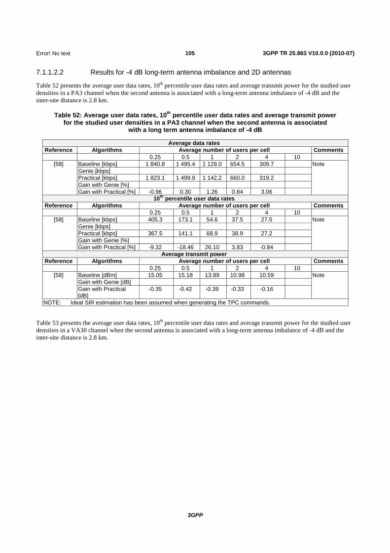
105
3GPP
Error! No text of specified
3GPP TR 25.863 V10.0.0 (2010-07)
7.1.1.2.2 Results for -4 dB long-term antenna imbalance and 2D antennas
Table 52 presents the average user data rates, 10th percentile user data rates and average transmit power for the studied user densities in a PA3 channel when the second antenna is associated with a long-term antenna imbalance of -4 dB and the inter-site distance is 2.8 km.
Table 52: Average user data rates, 10th percentile user data rates and average transmit power for the studied user densities in a PA3 channel when the second antenna is associated
with a long term antenna imbalance of -4 dB
Average data rates Reference Algorithms Average number of users per cell Comments
0.25 0.5 1 2 4 10 [58] Baseline [kbps] 1 840.8 1 495.4 1 128.0 654.5 309.7 Note
Genie [kbps] Practical [kbps] 1 823.1 1 499.9 1 142.2 660.0 319.2 Gain with Genie [%] Gain with Practical [%] -0.96 0.30 1.26 0.84 3.06
10th percentile user data rates Reference Algorithms Average number of users per cell Comments
0.25 0.5 1 2 4 10 [58] Baseline [kbps] 405.3 173.1 54.6 37.5 27.5 Note
Genie [kbps] Practical [kbps] 367.5 141.1 68.9 38.9 27.2 Gain with Genie [%] Gain with Practical [%] -9.32 -18.46 26.10 3.83 -0.84
Average transmit power Reference Algorithms Average number of users per cell Comments
0.25 0.5 1 2 4 10 [58] Baseline [dBm] 15.05 15.18 13.89 10.98 10.59 Note
Gain with Genie [dB] Gain with Practical [dB]
-0.35 -0.42 -0.39 -0.33 -0.16
NOTE: Ideal SIR estimation has been assumed when generating the TPC commands.
Table 53 presents the average user data rates, 10th percentile user data rates and average transmit power for the studied user densities in a VA30 channel when the second antenna is associated with a long-term antenna imbalance of -4 dB and the inter-site distance is 2.8 km.

106
3GPP
Error! No text of specified
3GPP TR 25.863 V10.0.0 (2010-07)
Table 53: Average user data rates, 10th percentile user data rates and average transmit power for the studied user densities in a VA30 channel when the second antenna is associated
with a long term antenna imbalance of -4 dB
Average data rates Reference Algorithms Average number of users per cell Comments
0.25 0.5 1 2 4 10 [58] Baseline [kbps] 1 530.8 1 282.9 989.0 636.4 335.8 Note
Genie [kbps] Practical [kbps] 1 511.7 1 265.5 990.2 639.4 338.4 Gain with Genie [%] Gain with Practical [%] -1.25 -1.36 0.12 0.47 0.77
10th percentile user data rates Reference Algorithms Average number of users per cell Comments
0.25 0.5 1 2 4 10 [58] Baseline [kbps] 318.7 210.6 65.3 26.5 32.2 Note
Genie [kbps] Practical [kbps] 284.0 192.7 61.4 18.4 25.3 Gain with Genie [%] Gain with Practical [%] -10.89 -8.50 -5.93 -30.41 -21.45
Average transmit power Reference Algorithms Average number of users per cell Comments
0.25 0.5 1 2 4 10 [58] Baseline [dBm] 16.03 14.68 13.58 11.97 9.27 Note
Gain with Genie [dB] Gain with Practical [dB]
-0.33 -0.39 -0.48 -0.44 -0.43
NOTE: Ideal SIR estimation has been assumed when generating the TPC commands.
7.1.1.2.3 Results for ISD 2.8 km with 50 % penetration of SATD terminals
Additional simulations were performed by one company to investigate the performance of SATD in a situation where the penetrations of UL TxD was only 50 %. In these simulations, all TX diversity UEs are assumed to use the same TxD algorithm. Other penetration levels have not been checked. The results suggest that:
- Where the penetration level is 50 %, there is no net system capacity gain from UL SATD.
- In a 2.8 km cell, the 10th percentile user throughput for non diversity users may be reduced.
Some inconsistencies were noted in the results.
Tables 54 and 55 present the average user data rates, the 10th percentile user data rates and the average transmit power for the different user densities that was studied for a PA3 channel when the inter-site distance is 2.8 km and only 50 % of the terminals are operating SATD (with the remaining 50 % being legacy terminals). Both absolute and relative numbers are presented. Table 54 presents the numbers for TX diversity terminals, and table 55 for legacy terminals. All relative numbers are presented with respect to baseline case (without transmit diversity for any terminals).

107
3GPP
Error! No text of specified
3GPP TR 25.863 V10.0.0 (2010-07)
Table 54: Average user data rates for TX diversity terminals, 10th percentile user data rates and average transmit power for the studied user densities in a PA3 channel
when the inter-site distance is 2.8 km and the penetration of SATD terminals is 50 %
Average data rates Reference Algorithms Average number of users per cell Comments
0.25 0.5 1 2 4 10 [73] Baseline [kbps] 1 258 899 524 194 Note
Genie [kbps] 1 350 972 560 209 Practical [kbps] 1 309 915 526 202 Gain with Genie [%] 7.3 8.1 6.3 7.7 Gain with Practical [%] 4 1.8 0.4 4.1
10th percentile user data rates Reference Algorithms Average number of users per cell Comments
0.25 0.5 1 2 4 10 [73] Baseline [kbps] 193 114 88 74 Note
Genie [kbps] 202 155 110 74 Practical [kbps] 185 119 85 75 Gain with Genie [%] 4.6 36 25 0 Gain with Practical [%] -4.1 4.4 -3.4 1.3
Average transmit power Reference Algorithms Average number of users per cell Comments
0.25 0.5 1 2 4 10 [73] Baseline [dBm] 20.07 19.63 19.01 17.61 Note
Gain with Genie [dB] 0.29 0.21 0.55 0.75 Gain with Practical [dB] 0.10 -0.12 -0.05 0.03
NOTE: Ideal SIR estimation has been assumed when generating the TPC commands.
Table 55: Average user data rates for legacy terminals, 10th percentile user data rates and average transmit power for the studied user densities in a PA3 channel
when the inter-site distance is 2.8 km and the penetration of SATD terminals is 50 %
Average data rates Reference Algorithms Average number of users per cell Comments
0.25 0.5 1 2 4 10 [73] Baseline [kbps] 1 258 899 524 194 Note
Genie [kbps] 1 244 906 529 197 Practical [kbps] 1 258 891 523 197 Gain with Genie [%] -1.1 0.7 1 1.5 Gain with Practical [%] 0 -0.9 -0.2 1.5
10th percentile user data rates Reference Algorithms Average number of users per cell Comments
0.25 0.5 1 2 4 10 [73] Baseline [kbps] 193 114 88 74 Note
Genie [kbps] 148 122 82 63 Practical [kbps] 158 95 92 69 Gain with Genie [%] -23 7 -7 -1.3 Gain with Practical [%] -18 -16.7 4.5 -6.7
Average transmit power Reference Algorithms Average number of users per cell Comments
0.25 0.5 1 2 4 10 [73] Baseline [dBm] 20.07 19.63 19.01 17.61 Note
Gain with Genie [dB] -0.13 -0.07 -0.13 -0.24 Gain with Practical [dB] -0.11 -0.20 -0.09 0.05
NOTE: Ideal SIR estimation has been assumed when generating the TPC commands.
Tables 56 and 57 presents the average user data rates, the 10th percentile user data rates and the average transmit power for the studied user densities in a VA30 channel when the inter-site distance is 1 km and only 50 % of the terminals are

108
3GPP
Error! No text of specified
3GPP TR 25.863 V10.0.0 (2010-07)
operating SATD (with the remaining 50 % being legacy terminals). Both absolute and relative numbers are presented. Table 56 presents the numbers for TX diversity terminals, and table 57 for legacy terminals. All relative numbers are presented with respect to baseline case (without transmit diversity for any terminals).
Table 56: Average user data rates for TX diversity terminals, 10th percentile user data rates and average transmit power for the studied user densities in a VA30 channel
when the inter-site distance is 2.8 km and the penetration of SATD terminals is 50 %
Average data rates Reference Algorithms Average number of users per cell Comments
0.25 0.5 1 2 4 10 [73] Baseline [kbps] 1 111 771 461 179 Note
Genie [kbps] 1 151 845 519 198 Practical [kbps] 1 107 759 451 176 Gain with Genie [%] 3.6 9.6 12.5 10.6 Gain with Practical [%] -0.4 -1.6 -2.2 -1.7
10th percentile user data rates Reference Algorithms Average number of users per cell Comments
0.25 0.5 1 2 4 10 [73] Baseline [kbps] 144 96 75 65 Note
Genie [kbps] 203 141 96 82 Practical [kbps] 171 108 66 51 Gain with Genie [%] 41 47 28 26 Gain with Practical [%] 18 12.5 -12 -21
Average transmit power Reference Algorithms Average number of users per cell Comments
0.25 0.5 1 2 4 10 [73] Baseline [dBm] 20.12 19.67 18.81 17.39 Note
Gain with Genie [dB] 0.45 0.28 0.31 0.76 Gain with Practical [dB] 0.11 0.01 -0.30 -0.16
NOTE: Ideal SIR estimation has been assumed when generating the TPC commands.

109
3GPP
Error! No text of specified
3GPP TR 25.863 V10.0.0 (2010-07)
Table 57: Average user data rates for legacy terminals, 10th percentile user data rates and average transmit power for the studied user densities in a VA30 channel
when the inter-site distance is 2.8 km and the penetration of SATD terminals is 50 %
Average data rates Reference Algorithms Average number of users per cell Comments
0.25 0.5 1 2 4 10 [73] Baseline [kbps] 1 111 771 461 179 Note
Genie [kbps] 1 064 799 476 191 Practical [kbps] 1 086 801 488 177 Gain with Genie [%] -4.4 3.6 3.2 6.7 Gain with Practical [%] -2.2 3.9 5.9 -1.1
10th percentile user data rates Reference Algorithms Average number of users per cell Comments
0.25 0.5 1 2 4 10 [73] Baseline [kbps] 144 96 75 65 Note
Genie [kbps] 148 88 78 69 Practical [kbps] 137 91 70 51 Gain with Genie [%] 2.7 -8.3 -4 6.1 Gain with Practical [%] -4.9 -5.2 -6.7 -21
Average transmit power Reference Algorithms Average number of users per cell Comments
0.25 0.5 1 2 4 10 [73] Baseline [dBm] 20.12 19.67 18.81 17.39 Note
Gain with Genie [dB] -0.06 0.05 -0.06 0.01 Gain with Practical [dB] 0.09 -0.01 -0.05 -0.07
Note 1: Ideal SIR estimation has been assumed when generating the TPC commands.
7.1.1.2.4 Results for 0 dB long-term antenna imbalance and 2D antennas with 25 % penetration of SATD terminals and 2 800 m ISD
Additional simulations were performed by one company to investigate the performance of SATD in a situation where the penetrations of UL TxD was only 25 %. In these simulations, all TX diversity UEs are assumed to use the same TxD algorithm. Only 25 % of the terminals are operating SATD with the remaining 75 % being legacy, non TX-diversity terminals. The results are split to three sub-sections, first including the total cell throughputs and two latter looking at the performance of TX-diversity and non TX-diversity users separately.
The results suggest that for 2.8 km ISD:
- Where the penetration level is 25 %, there is no net system capacity gain or loss from UL SATD with non-ideal algorithms.
- Depending on the load the average user throughput in increased or decreased for both user groups.
- Depending on the load the 10th percentile throughput is improved for the TX-diversity users, while average transmit power does not show significant difference compared to the baseline.
- Depending on the load the 10th percentile throughput of non TX-diversity users is either increased or decreased, however some loss was seen at VA30 channel.

110
3GPP
Error! No text of specified
3GPP TR 25.863 V10.0.0 (2010-07)
7.1.1.2.4.1 Results for all users
Tables 57a1 presents the cell throughput results for the studied user densities in a PA3 channel when the inter-site distance is 1 km for the SATD terminals. Both absolute and relative numbers are presented Results in VA30 channel are given in table 57a2.
Table 57a1: Cell throughputs in a PA3 channel when the inter-site distance is 2.8 km and the penetration of SATD terminals is 25 %
Cell throughput Reference Algorithms Average number of users per cell Comments
0.25 0.5 1 2 4 10 [81] Baseline [kbps] 1 258,44 1 798,31 2 096,90 1 947,27
Genie [kbps] 1 252,45 1 814,24 2 144,42 1 987,05 Practical [kbps] 1 233,16 1 786,55 2 112,72 1 950,90 Gain with Genie [%] -0,48 0,89 2,27 2,04 Gain with Practical [%] -2,01 -0,65 0,75 0,19
Table 57a2: Cell throughputs in a VA30 channel when the inter-site distance is 2.8 km and the penetration of SATD terminals is 25 %
Cell throughput Reference Algorithms Average number of users per cell Comments
0.25 0.5 1 2 4 10 [81] Baseline [kbps] 1 111,32 1 544,02 1 847,53 1 793,56
Genie [kbps] 1 099,97 1 597,88 1 908,42 1 793,62 Practical [kbps] 1 094,85 1 592,18 1 903,81 1 790,62 Gain with Genie [%] -1,02 3,49 3,30 0,00 Gain with Practical [%] -1,48 3,12 3,05 -0,16
7.1.1.2.4.2 Results for TX-diversity users
Tables 57b1, 57b2 and 57b3 presents the average user data rates, the 10th percentile user data rates and the average transmit power for the studied user densities in a PA3 channel when the inter-site distance is 2.8 km for the SATD terminals. Both absolute and relative numbers are presented. All relative numbers are presented with respect to baseline case (without transmit diversity for any terminals). Tables 57b4, 57b5 and 57b6 include the results for VA30 channel.
Table 57b1: Average user data rates for TX diversity terminals for the studied user densities in a PA3 channel when the inter-site distance is 2.8 km and the penetration
of SATD terminals is 25 %
Average data rates Reference Algorithms Average number of users per cell Comments
0.25 0.5 1 2 4 10 [81] Baseline [kbps] 1 258,53 899,13 524,24 194,71
Genie [kbps] 1 332,57 957,86 550,71 205,99 Practical [kbps] 1 250,30 901,29 523,57 197,95 Gain with Genie [%] 5,88 6,53 5,05 5,80 Gain with Practical [%] -0,65 0,24 -0,13 1,67

111
3GPP
Error! No text of specified
3GPP TR 25.863 V10.0.0 (2010-07)
Table 57b2: 10th percentile user data rates for TX diversity terminals for the studied user densities in a PA3 channel when the inter-site distance is 2.8 km and the penetration
of SATD terminals is 25 %
10th percentile user data rates Reference Algorithms Average number of users per cell Comments
0.25 0.5 1 2 4 10 [81] Baseline [kbps] 95,98 56,67 40,29 40,05
Genie [kbps] 117,84 75,37 57,43 53,13 Practical [kbps] 98,15 60,06 48,18 44,88 Gain with Genie [%] 22,78 33,00 42,55 32,67 Gain with Practical [%] 2,26 5,99 19,59 12,07
Table 57b3: average transmit power for TX diversity terminals for the studied user densities in a PA3 channel when the inter-site distance is 2.8 km and the penetration
of SATD terminals is 25 %
Average transmit power Reference Algorithms Average number of users per cell Comments
0.25 0.5 1 2 4 10 [81] Baseline [kbps] 20,07 19,63 19,01 17,61
Gain with Genie [dB] 0,21 0,26 0,41 0,82 Gain with Practical [dB] 0,00 -0,02 0,02 0,25
Table 57b4: Average user data rates for TX diversity terminals for the studied user densities in a VA30 channel when the inter-site distance is 2.8 km and the penetration
of SATD terminals is 25 %
Average data rates Reference Algorithms Average number of users per cell Comments
0.25 0.5 1 2 4 10 [81] Baseline [kbps] 1 111,33 771,91 461,88 179,34
Genie [kbps] 1 099,49 806,86 482,91 181,41 Practical [kbps] 1 071,45 788,35 473,44 179,14 Gain with Genie [%] -1,07 4,53 4,55 1,15 Gain with Practical [%] -3,59 2,13 2,50 -0,11
Table 57b5: 10th percentile user data rates for TX diversity terminals for the studied user densities in a VA30 channel when the inter-site distance is 2.8 km and the penetration
of SATD terminals is 25 %
10th percentile user data rates Reference Algorithms Average number of users per cell Comments
0.25 0.5 1 2 4 10 [81] Baseline [kbps] 76,97 49,53 39,48 36,68
Genie [kbps] 75,14 53,27 43,94 33,09 Practical [kbps] 66,65 47,67 40,06 28,67 Gain with Genie [%] -2,37 7,56 11,30 -9,79 Gain with Practical [%] -13,41 -3,75 1,46 -21,85
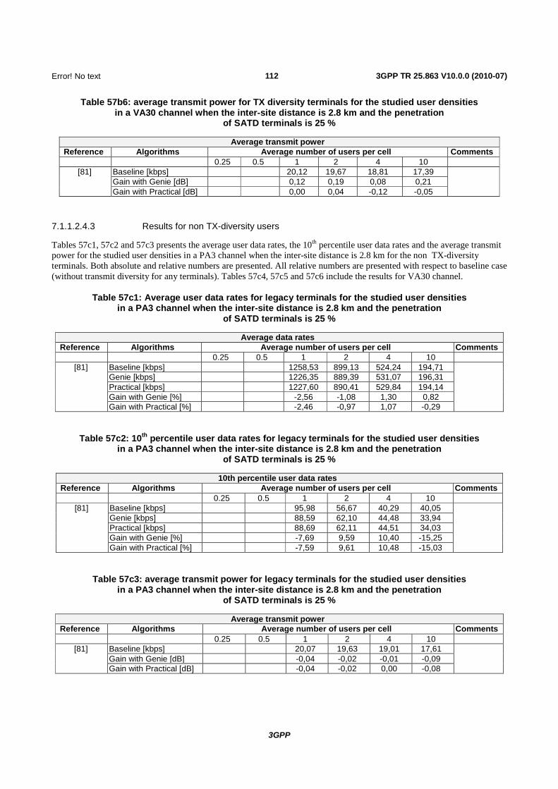
112
3GPP
Error! No text of specified
3GPP TR 25.863 V10.0.0 (2010-07)
Table 57b6: average transmit power for TX diversity terminals for the studied user densities in a VA30 channel when the inter-site distance is 2.8 km and the penetration
of SATD terminals is 25 %
Average transmit power Reference Algorithms Average number of users per cell Comments
0.25 0.5 1 2 4 10 [81] Baseline [kbps] 20,12 19,67 18,81 17,39
Gain with Genie [dB] 0,12 0,19 0,08 0,21 Gain with Practical [dB] 0,00 0,04 -0,12 -0,05
7.1.1.2.4.3 Results for non TX-diversity users
Tables 57c1, 57c2 and 57c3 presents the average user data rates, the 10th percentile user data rates and the average transmit power for the studied user densities in a PA3 channel when the inter-site distance is 2.8 km for the non TX-diversity terminals. Both absolute and relative numbers are presented. All relative numbers are presented with respect to baseline case (without transmit diversity for any terminals). Tables 57c4, 57c5 and 57c6 include the results for VA30 channel.
Table 57c1: Average user data rates for legacy terminals for the studied user densities in a PA3 channel when the inter-site distance is 2.8 km and the penetration
of SATD terminals is 25 %
Average data rates Reference Algorithms Average number of users per cell Comments
0.25 0.5 1 2 4 10 [81] Baseline [kbps] 1258,53 899,13 524,24 194,71
Genie [kbps] 1226,35 889,39 531,07 196,31 Practical [kbps] 1227,60 890,41 529,84 194,14 Gain with Genie [%] -2,56 -1,08 1,30 0,82 Gain with Practical [%] -2,46 -0,97 1,07 -0,29
Table 57c2: 10th percentile user data rates for legacy terminals for the studied user densities in a PA3 channel when the inter-site distance is 2.8 km and the penetration
of SATD terminals is 25 %
10th percentile user data rates Reference Algorithms Average number of users per cell Comments
0.25 0.5 1 2 4 10 [81] Baseline [kbps] 95,98 56,67 40,29 40,05
Genie [kbps] 88,59 62,10 44,48 33,94 Practical [kbps] 88,69 62,11 44,51 34,03 Gain with Genie [%] -7,69 9,59 10,40 -15,25 Gain with Practical [%] -7,59 9,61 10,48 -15,03
Table 57c3: average transmit power for legacy terminals for the studied user densities in a PA3 channel when the inter-site distance is 2.8 km and the penetration
of SATD terminals is 25 %
Average transmit power Reference Algorithms Average number of users per cell Comments
0.25 0.5 1 2 4 10 [81] Baseline [kbps] 20,07 19,63 19,01 17,61
Gain with Genie [dB] -0,04 -0,02 -0,01 -0,09 Gain with Practical [dB] -0,04 -0,02 0,00 -0,08

113
3GPP
Error! No text of specified
3GPP TR 25.863 V10.0.0 (2010-07)
Table 57c4: Average user data rates for legacy terminals for the studied user densities in a VA30 channel when the inter-site distance is 2.8 km and the penetration
of SATD terminals is 25 %
Average data rates Reference Algorithms Average number of users per cell Comments
0.25 0.5 1 2 4 10 [81] Baseline [kbps] 1 111,33 771,91 461,88 179,34
Genie [kbps] 1 100,17 796,21 475,21 178,70 Practical [kbps] 1 102,51 798,58 476,74 179,05 Gain with Genie [%] -1,00 3,15 2,88 -0,36 Gain with Practical [%] -0,79 3,45 3,22 -0,16
Table 57c5: 10th percentile user data rates for legacy terminals for the studied user densities in a VA30 channel when the inter-site distance is 2.8 km and the penetration
of SATD terminals is 25 %
10th percentile user data rates Reference Algorithms Average number of users per cell Comments
0.25 0.5 1 2 4 10 [81] Baseline [kbps] 76,97 49,53 39,48 36,68
Genie [kbps] 70,08 48,24 33,66 28,58 Practical [kbps] 70,04 47,98 33,44 28,43 Gain with Genie [%] -8,95 -2,60 -14,74 -22,10 Gain with Practical [%] -9,00 -3,14 -15,31 -22,50
Table 57c6: average transmit power for legacy terminals for the studied user densities in a VA30 channel when the inter-site distance is 2.8 km and the penetration
of SATD terminals is 25 %
Average transmit power Reference Algorithms Average number of users per cell Comments
0.25 0.5 1 2 4 10 [81] Baseline [kbps] 20,12 19,67 18,81 17,39
Gain with Genie [dB] 0,01 0,03 -0,14 -0,19 Gain with Practical [dB] 0,00 0,02 -0,14 -0,19
7.1.1.2.5 Results for 0 dB long-term antenna imbalance and 2D antennas with 75 % penetration of SATD terminals and 2 800 m ISD
Additional simulations were performed by one company to investigate the performance of SATD in a situation where the penetrations of UL TxD was 75 %. In these simulations, all TX diversity UEs are assumed to use the same TxD algorithm. 75 % of the terminals are operating SATD with the remaining 25 % being legacy, non TX-diversity terminals. The results are split to three sub-sections, first including the total cell throughputs and two latter looking at the performance of TX-diversity and non TX-diversity users separately.
The results suggest that for 2.8 km ISD:
- Where the penetration level is 75 %, there is no net system capacity gain from UL SATD with non-ideal algorithms
- Depending on the load the average user throughput in increased or decreased for both user groups.
- The load the 10th percentile throughput is either improved or decreased depending on the load and channel condition.

114
3GPP
Error! No text of specified
3GPP TR 25.863 V10.0.0 (2010-07)
7.1.1.2.5.1 Results for all users
Tables 57d1 presents the cell throughput results for the studied user densities in a PA3 channel when the inter-site distance is 1 km for the SATD terminals. Both absolute and relative numbers are presented Results in VA30 channel are given in table 57d2.
Table 57d1: Cell throughputs in a PA3 channel when the inter-site distance is 2.8 km and the penetration of SATD terminals is 75 %
Cell throughput Reference Algorithms Average number of users per cell Comments
0.25 0.5 1 2 4 10 Baseline [kbps] 1 258,44 1 798,31 2 096,90 1 947,27
Genie [kbps] 1 319,42 1 903,29 2 241,73 2 108,48 Practical [kbps] 1 261,05 1 820,57 2 145,73 2 002,85 Gain with Genie [%] 4,85 5,84 6,91 8,28 Gain with Practical [%] 0,21 1,24 2,33 2,85
Table 57d2: Cell throughputs in a VA30 channel when the inter-site distance is 2.8 km and the penetration of SATD terminals is 75 %.
Cell throughput Reference Algorithms Average number of users per cell Comments
0.25 0.5 1 2 4 10 Baseline [kbps] 1 111,32 1 544,02 1 847,53 1 793,56 Genie [kbps] 1 125,41 1 591,93 1 914,74 1 812,47 Practical [kbps] 1 108,94 1 574,83 1 900,43 1 804,17 Gain with Genie [%] 1,27 3,10 3,64 1,05 Gain with Practical [%] -0,21 2,00 2,86 0,59
7.1.1.2.5.2 Results for TX-diversity users
Tables 57e1, 57e2 and 57e3 presents the average user data rates, the 10th percentile user data rates and the average transmit power for the studied user densities in a PA3 channel when the inter-site distance is 2.8 km for the SATD terminals. Both absolute and relative numbers are presented. All relative numbers are presented with respect to baseline case (without transmit diversity for any terminals). Tables 57e4, 57e5 and 57e6 include the results for VA30 channel.
Table 57e1: Average user data rates for TX diversity terminals for the studied user densities in a PA3 channel when the inter-site distance is 2.8 km and the penetration
of SATD terminals is 75 %
Average data rates Reference Algorithms Average number of users per cell Comments
0.25 0.5 1 2 4 10 [81] Baseline [kbps] 1 258,53 899,13 524,24 194,71
Genie [kbps] 1 353,89 974,66 567,38 211,45 Practical [kbps] 1 274,22 919,13 537,23 199,43 Gain with Genie [%] 7,58 8,40 8,23 8,60 Gain with Practical [%] 1,25 2,23 2,48 2,43

115
3GPP
Error! No text of specified
3GPP TR 25.863 V10.0.0 (2010-07)
Table 57e2: 10th percentile user data rates for TX diversity terminals for the studied user densities in a PA3 channel when the inter-site distance is 2.8 km and the penetration
of SATD terminals is 75 %
10th percentile user data rates Reference Algorithms Average number of users per cell Comments
0.25 0.5 1 2 4 10 [81] Baseline [kbps] 95,98 56,67 40,29 40,05
Genie [kbps] 121,39 87,93 61,73 48,60 Practical [kbps] 99,27 69,19 49,14 37,03 Gain with Genie [%] 26,48 55,18 53,22 21,36 Gain with Practical [%] 3,43 22,10 21,96 -7,54
Table 57e3: average transmit power for TX diversity terminals for the studied user densities in a PA3 channel when the inter-site distance is 2.8 km and the penetration
of SATD terminals is 75 %
Average transmit power Reference Algorithms Average number of users per cell Comments
0.25 0.5 1 2 4 10 [81] Baseline [kbps] 20,07 19,63 19,01 17,61
Gain with Genie [dB] 0,29 0,36 0,57 0,67 Gain with Practical [dB] 0,07 0,08 0,21 0,16
Table 57e4: Average user data rates for TX diversity terminals for the studied user densities in a VA30 channel when the inter-site distance is 2.8 km and the penetration
of SATD terminals is 75 %
Average data rates Reference Algorithms Average number of users per cell Comments
0.25 0.5 1 2 4 10 [81] Baseline [kbps] 1 111,33 771,91 461,88 179,34
Genie [kbps] 1 127,74 804,50 481,84 182,26 Practical [kbps] 1 103,32 790,74 475,42 180,79 Gain with Genie [%] 1,48 4,22 4,32 1,63 Gain with Practical [%] -0,72 2,44 2,93 0,81
Table 57e5: 10th percentile user data rates for TX diversity terminals for the studied user densities in a VA30 channel when the inter-site distance is 2.8 km and the penetration
of SATD terminals is 75 %
10th percentile user data rates Reference Algorithms Average number of users per cell Comments
0.25 0.5 1 2 4 10 [81] Baseline [kbps] 76,97 49,53 39,48 36,68
Genie [kbps] 81,43 52,10 39,05 30,44 Practical [kbps] 71,55 48,31 34,29 30,70 Gain with Genie [%] 5,80 5,18 -1,09 -17,01 Gain with Practical [%] -7,04 -2,47 -13,16 -16,32

116
3GPP
Error! No text of specified
3GPP TR 25.863 V10.0.0 (2010-07)
Table 57e6: average transmit power for TX diversity terminals for the studied user densities in a VA30 channel when the inter-site distance is 2.8 km and the penetration
of SATD terminals is 75 %
Average transmit power Reference Algorithms Average number of users per cell Comments
0.25 0.5 1 2 4 10 [81] Baseline [kbps] 20,12 19,67 18,81 17,39
Gain with Genie [dB] 0,14 0,22 0,09 0,23 Gain with Practical [dB] 0,02 0,06 -0,10 -0,02
7.1.1.2.5.3 Results for non TX-diversity users
Tables 57f1, 57f2 and 57f3 presents the average user data rates, the 10th percentile user data rates and the average transmit power for the studied user densities in a PA3 channel when the inter-site distance is 2.8 km for the non TX-diversity terminals. Both absolute and relative numbers are presented. All relative numbers are presented with respect to baseline case (without transmit diversity for any terminals). Tables 57f4, 57f5 and 57f6 include the results for VA30 channel.
Table 57f1: Average user data rates for legacy terminals for the studied user densities in a PA3 channel when the inter-site distance is 2.8 km and the penetration
of SATD terminals is 75 %
Average data rates Reference Algorithms Average number of users per cell Comments
0.25 0.5 1 2 4 10 [81] Baseline [kbps] 1 258,53 899,13 524,24 194,71
Genie [kbps] 1 217,10 879,67 538,60 209,07 Practical [kbps] 1 222,02 882,37 533,90 202,74 Gain with Genie [%] -3,29 -2,16 2,74 7,38 Gain with Practical [%] -2,90 -1,86 1,84 4,12
Table 57f2: 10th percentile user data rates for legacy terminals for the studied user densities in a PA3 channel when the inter-site distance is 2.8 km and the penetration
of SATD terminals is 75 %
10th percentile user data rates Reference Algorithms Average number of users per cell Comments
0.25 0.5 1 2 4 10 [81] Baseline [kbps] 95,98 56,67 40,29 40,05
Genie [kbps] 89,73 61,55 47,25 36,10 Practical [kbps] 90,33 60,83 47,12 37,39 Gain with Genie [%] -6,51 8,62 17,28 -9,87 Gain with Practical [%] -5,88 7,34 16,94 -6,63
Table 57f3: average transmit power for legacy terminals for the studied user densities in a PA3 channel when the inter-site distance is 2.8 km and the penetration
of SATD terminals is 75 %
Average transmit power Reference Algorithms Average number of users per cell Comments
0.25 0.5 1 2 4 10 [81] Baseline [kbps] 20,07 19,63 19,01 17,61
Gain with Genie [dB] -0,08 -0,10 -0,07 -0,19 Gain with Practical [dB] -0,08 -0,10 -0,04 -0,14

117
3GPP
Error! No text of specified
3GPP TR 25.863 V10.0.0 (2010-07)
Table 57f4: Average user data rates for legacy terminals for the studied user densities in a VA30 channel when the inter-site distance is 2.8 km and the penetration
of SATD terminals is 75 %
Average data rates Reference Algorithms Average number of users per cell Comments
0.25 0.5 1 2 4 10 [81] Baseline [kbps] 1 111,33 771,91 461,88 179,34
Genie [kbps] 1 118,39 770,49 469,29 178,23 Practical [kbps] 1 125,19 777,84 474,30 179,37 Gain with Genie [%] 0,64 -0,18 1,60 -0,62 Gain with Practical [%] 1,25 0,77 2,69 0,01
Table 57f5: 10th percentile user data rates for legacy terminals for the studied user densities in a VA30 channel when the inter-site distance is 2.8 km and the penetration
of SATD terminals is 75 %
10th percentile user data rates Reference Algorithms Average number of users per cell Comments
0.25 0.5 1 2 4 10 [81] Baseline [kbps] 76,97 49,53 39,48 36,68
Genie [kbps] 85,52 50,39 34,23 26,41 Practical [kbps] 84,63 50,34 34,46 26,86 Gain with Genie [%] 11,11 1,73 -13,30 -28,00 Gain with Practical [%] 9,96 1,63 -12,72 -26,77
Table 57f6: average transmit power for legacy terminals for the studied user densities in a VA30 channel when the inter-site distance is 2.8 km and the penetration
of SATD terminals is 75 %
Average transmit power Reference Algorithms Average number of users per cell Comments
0.25 0.5 1 2 4 10 [81] Baseline [kbps] 20,12 19,67 18,81 17,39
Gain with Genie [dB] 0,13 0,13 -0,13 -0,15 Gain with Practical [dB] 0,12 0,11 -0,14 -0,14
7.1.1.3 Sensitivity to BLER target
The results presented in previous sections are based on the parameters presented in section 5.3.2. In particular, all except [49] are based on a setting where the residual BLER target after the 4th transmission is 1 %. The subsection evaluates the relative gain in average data rates of the practical antenna switching algorithm (with respect to the base line case). This is presented in figure 29 for two different loads. From the figure it can be observed that the performance gain stemming from antenna switching algorithms reduce as the BLER target becomes more stringent.
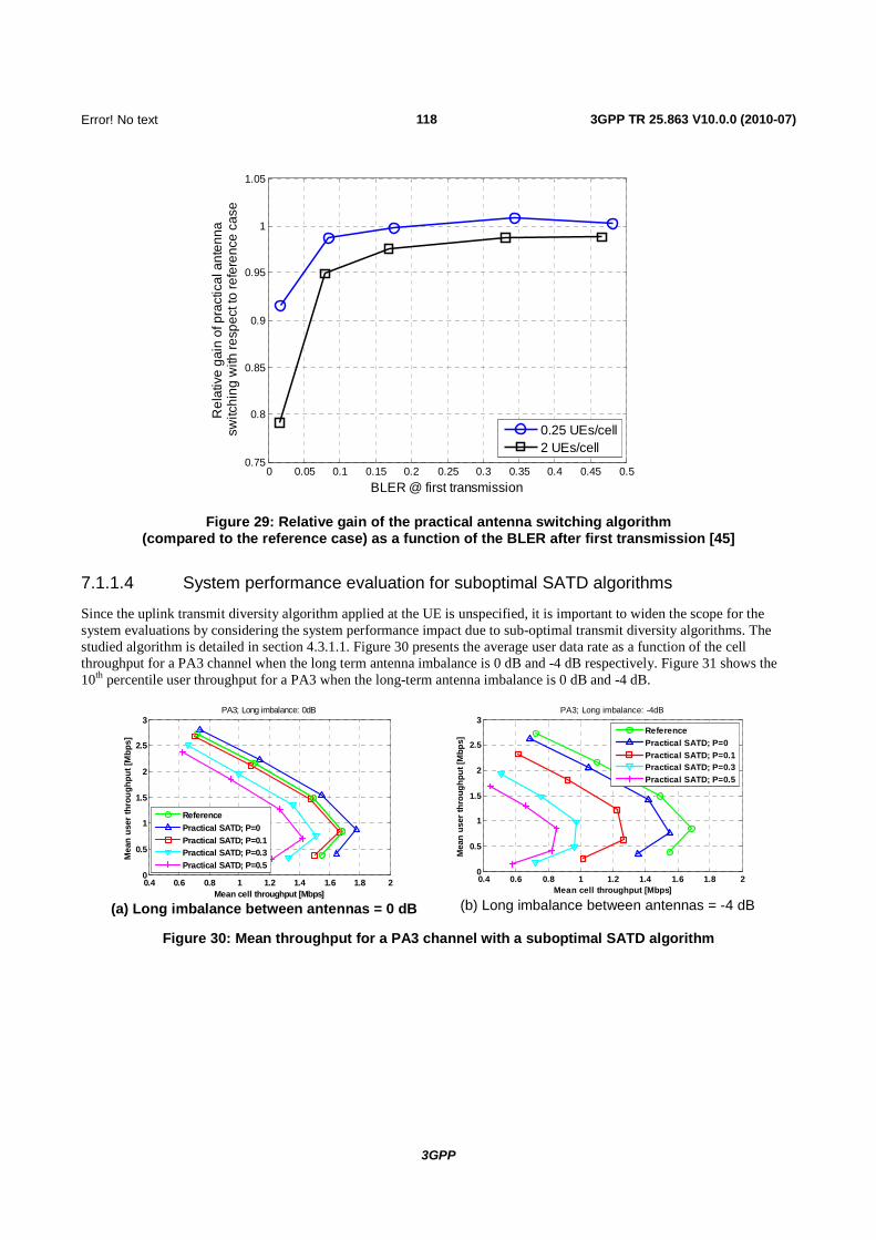
118
3GPP
Error! No text of specified
3GPP TR 25.863 V10.0.0 (2010-07)
0 0.05 0.1 0.15 0.2 0.25 0.3 0.35 0.4 0.45 0.50.75
0.8
0.85
0.9
0.95
1
1.05
BLER @ first transmission
Rel
ativ
e ga
in o
f pra
ctic
al a
nten
na
switc
hing
with
resp
ect t
o re
fere
nce
case
0.25 UEs/cell2 UEs/cell
Figure 29: Relative gain of the practical antenna switching algorithm (compared to the reference case) as a function of the BLER after first transmission [45]
7.1.1.4 System performance evaluation for suboptimal SATD algorithms
Since the uplink transmit diversity algorithm applied at the UE is unspecified, it is important to widen the scope for the system evaluations by considering the system performance impact due to sub-optimal transmit diversity algorithms. The studied algorithm is detailed in section 4.3.1.1. Figure 30 presents the average user data rate as a function of the cell throughput for a PA3 channel when the long term antenna imbalance is 0 dB and -4 dB respectively. Figure 31 shows the 10th percentile user throughput for a PA3 when the long-term antenna imbalance is 0 dB and -4 dB.
0.4 0.6 0.8 1 1.2 1.4 1.6 1.8 20
0.5
1
1.5
2
2.5
3PA3; Long imbalance: 0dB
Mean cell throughput [Mbps]
Mea
n u
ser
thro
ug
hp
ut
[Mb
ps]
ReferencePractical SATD; P=0Practical SATD; P=0.1Practical SATD; P=0.3Practical SATD; P=0.5
(a) Long imbalance between antennas = 0 dB
0.4 0.6 0.8 1 1.2 1.4 1.6 1.8 20
0.5
1
1.5
2
2.5
3PA3; Long imbalance: -4dB
Mean cell throughput [Mbps]
Mea
n u
ser
thro
ugh
put [
Mbp
s]
ReferencePractical SATD; P=0Practical SATD; P=0.1Practical SATD; P=0.3Practical SATD; P=0.5
(b) Long imbalance between antennas = -4 dB
Figure 30: Mean throughput for a PA3 channel with a suboptimal SATD algorithm

119
3GPP
Error! No text of specified
3GPP TR 25.863 V10.0.0 (2010-07)
0.25 0.5 1 2 40
0.2
0.4
0.6
0.8
1
1.2
1.4PA3; Long imbalance: 0dB
Average number of users per cell
10th
per
cen
tile
use
r th
rou
ghp
ut[
Mbp
s]
ReferencePractical SATD; P=0Practical SATD; P=0.1Practical SATD; P=0.3Practical SATD; P=0.5
(a) Long imbalance between antennas = 0 dB
0.25 0.5 1 2 40
0.2
0.4
0.6
0.8
1
1.2
1.4PA3; Long imbalance: -4dB
Average number of users per cell
10th
per
cen
tile
use
r th
rou
gh
pu
t[M
bps
]
ReferencePractical SATD; P=0Practical SATD; P=0.1Practical SATD; P=0.3Practical SATD; P=0.5
(b) Long imbalance between antennas = -4 dB
Figure 31: Cell edge user throughput for a PA3 channel with a suboptimal SATD algorithm

120
3GPP
Error! No text of specified
3GPP TR 25.863 V10.0.0 (2010-07)
7.1.2 Bursty Traffic
7.1.2.1 Results for inter-site distance 1 km
7.1.2.1.1 Results for 0 dB long-term antenna imbalance and 2D antennas
Table 58, 58a, 58b and 58c presents the average user burst rates, the 10th percentile user burst rates and the average transmit power for the studied user densities in a PA3 channel with mean burst sizes of 125 KBytes, 30 KBytes, 5 KBytes and 1.25 KBytes respectively.
Table 58: Average user burst rates, 10th percentile user burst rates and average transmit power for the studied user densities in a PA3 channel when the inter-site distance is 1 km
with mean burst size 125 KBytes
Average user burst rate Reference Algorithms Average number of users per cell Comments
Penetration Loss [dB]
1 2 4 5 6
[75]
Baseline [Mbps]
10
6.09 5.39 4.04 3.29 Notes 1, 2 and 3
Practical [Mbps] 6.20 5.51 4.16 3.41 Gain with Practical [%]
1.79 2.11 2.96 3.72
[77]
Baseline [kbps]
10
1 071.07 1 070.25 1 072.72 1 041.11 Note 4 Note 5 Note 7
Practical [kbps] 1 095.81 1 095.01 1 096.80 1 074.19 Gain with Practical [%]
2.31 2.32 2.25 3.17
[75]
Baseline [Mbps]
20
4.67 4.20 3.25 2.72 Notes 1, 2 and 3
Practical [Mbps] 4.86 4.39 3.42 2.85 Gain with Practical [%]
4.23 4.63 5.37 4.93
[77]
Baseline [kbps]
20
1037.3 1028.1 1011.2 964.23 Note 4 Note 5 Note 7
Practical [kbps] 1064.1 1057.2 1043.3 1010.4 Gain with Practical [%]
2.59 2.83 3.18 4.79
10th percentile user burst rates Reference Algorithms Average number of users per cell Comments
Penetration Loss [dB]
1 2 4 5 6
[75]
Baseline [Mbps]
10
4.85 4.33 3.15 2.40 Notes 1, 2 and 3
Practical [Mbps] 4.97 4.43 3.28 2.53 Gain with Practical [%]
2.38 2.32 4.16 5.27
[77]
Baseline [Mbps]
10
996.03 996.39 998.31 959.63 Note 4 Note 5 Note 7
Practical [Mbps] 1 022.50 1 022.33 1 023.21 996.61 Gain with Practical [%]
2.66 2.60 2.50 3.85
[75]
Baseline [Mbps]
20
1.31 1.09 0.80 0.66 Notes 1, 2 and 3
Practical [Mbps] 1.54 1.29 0.98 0.80 Gain with Practical [%]
17.22 19.15 21.97 21.61
[77]
Baseline [kbps]
20
955.4 939.2 874.8 654.76 Note 4 Note 5 Note 7
Practical [kbps] 987.3 979.2 959.2 854.0 Gain with Practical [%]
3.34 4.26 9.65 30.42

121
3GPP
Error! No text of specified
3GPP TR 25.863 V10.0.0 (2010-07)
Average transmit power (dBm) Reference Algorithms Average number of users per cell Comments
1 2 4 5 6
[75] Baseline [dBm]
10 -17.26 -16.42 -14.86 -14.06 Notes 1, 2
and 3 Gain with Practical[dB] 1.07 1.08 1.01 0.98
[77] Baseline [dBm]
10 -18.97 -18.42 -17.04 -15.07 Note 4
Note 5 Note 7
Gain with Practical[dB] 1.61 1.73 1.89 2.13
[75] Baseline [dBm]
20 -7.56 -6.89 -5.62 -4.90 Notes 1, 2
and 3 Gain with Practical[dB] 1.07 1.11 1.04 1.03
[77] Baseline [dBm]
20 -8.83 -8.23 -6.97 -5.08 Note 4
Note 5 Note 7
Gain with Practical[dB] 1.69 1.84 1.94 2.11
NOTE 1: Noise Rise Target = 7 dB. NOTE 2: Target 10 % BLER after 1st transmission with a maximum of 4 transmissions. NOTE 3: NodeB Receiver: LMMSE Equalizer. NOTE 4: Target 1 % BLER after 4th transmission with a maximum of 4 transmissions. NOTE 5: NodeB Receiver: Rake. NOTE 6: Simulation assumes UE Category 7. NOTE 7: Simulation assumes UE Category 6.
Table 58a: Average user burst rates, 10th percentile user burst rates and average transmit power for the studied user densities in a PA3 channel when the inter-site distance is 1 km
with mean burst size 30 KBytes
Average user burst rate Reference Algorithms Average number of users per cell Comments
Penetration Loss [dB]
1 2 4 5 6
[77]
Baseline [kbps]
10
936.14 937.42 948.08 923.54 Note 4 Note 5 Note 7
Practical [kbps] 962.19 963.72 973.63 953.07 Gain with Practical [%]
2.78 2.81 2.70 3.20
[77]
Baseline [kbps]
20
912.25 906.94 897.45 854.38 Note 4 Note 5 Note 7
Practical [kbps] 938.79 935.26 928.41 897.34 Gain with Practical [%]
2.91 3.12 3.42 5.03
10th percentile user burst rates Reference Algorithms Average number of users per cell Comments
Penetration Loss [dB]
1 2 4 5 6
[77]
Baseline [kbps]
10
892.40 894.46 906.28 882.49 Note 4 Note 5 Note 7
Practical [kbps] 919.94 923.14 931.38 913.93 Gain with Practical [%]
3.09 3.21 2.77 3.56
[77]
Baseline [kbps]
20
879.22 874.94 827.26 608.12 Note 4 Note 5 Note 7
Practical [kbps] 908.71 906.46 904.64 798.58 Gain with Practical [%]
3.36 3.60 9.36 31.32

122
3GPP
Error! No text of specified
3GPP TR 25.863 V10.0.0 (2010-07)
Average transmit power (dBM) Reference Algorithms Average number of users per cell Comments
1 2 4 5 6
[77] Baseline [dBm]
10 -19.04 -18.50 -17.07 -15.04 Note 4
Note 5 Note 7
Gain with Practical[dB] 1.62 1.73 1.89 2.17
[77] Baseline [dBm]
20 -8.93 -8.34 -6.98 -5.05 Note 4
Note 5 Note 7
Gain with Practical[dB] 1.69 1.84 1.95 2.15
NOTE 1: Noise Rise Target = 7 dB. NOTE 2: Target 10 % BLER after 1st transmission with a maximum of 4 transmissions. NOTE 3: NodeB Receiver: LMMSE Equalizer. NOTE 4: Target 1 % BLER after 4th transmission with a maximum of 4 transmissions. NOTE 5: NodeB Receiver: Rake. NOTE 6: Simulation assumes UE Category 7. NOTE 7: Simulation assumes UE Category 6.
Table 58b: Average user burst rates, 10th percentile user burst rates and average transmit power for the studied user densities in a PA3 channel when the inter-site distance is 1 km
with mean burst size 5 KBytes
Average user burst rate Reference Algorithms Average number of users per cell Comments
Penetration Loss [dB]
1 2 4 5 6
[77]
Baseline [kbps]
10
629.71 631.06 625.60 589.31 Note 4 Note 5 Note 7
Practical [kbps] 641.73 643.24 639.58 612.38 Gain with Practical [%]
1.90 1.93 2.23 3.91
[77]
Baseline [kbps]
20
617.32 614.97 594.40 545.24 Note 4 Note 5 Note 7
Practical [kbps] 628.94 627.14 612.19 576.83 Gain with Practical [%]
1.88 1.98 3.0 5.79
10th percentile user burst rates Reference Algorithms Average number of users per cell Comments
Penetration Loss [dB]
1 2 4 5 6
[77]
Baseline [kbps]
10
607.65 610.09 602.54 561.53 Note 4 Note 5 Note 7
Practical [kbps] 621.01 623.15 617.12 588.38 Gain with Practical [%]
2.20 2.14 2.42 4.78
[77]
Baseline [kbps]
20
603.59 603.86 574.42 438.15 Note 4 Note 5 Note 7
Practical [kbps] 616.20 616.77 598.03 517.63 Gain with Practical [%]
2.09 2.14 4.11 18.14

123
3GPP
Error! No text of specified
3GPP TR 25.863 V10.0.0 (2010-07)
Average transmit power (dBM) Reference Algorithms Average number of users per cell Comments
1 2 4 5 6
[77] Baseline [dBm]
10 -18.82 -18.30 -16.75 -14.71 Note 4
Note 5 Note 7
Gain with Practical[dB] 1.58 1.68 1.77 2.01
[77] Baseline [dBm]
20 -8.73 -8.15 -6.70 -4.69 Note 4
Note 5 Note 7
Gain with Practical[dB] 1.68 1.81 1.88 2.06
NOTE 1: Noise Rise Target = 7 dB. NOTE 2: Target 10 % BLER after 1st transmission with a maximum of 4 transmissions. NOTE 3: NodeB Receiver: LMMSE Equalizer. NOTE 4: Target 1 % BLER after 4th transmission with a maximum of 4 transmissions. NOTE 5: NodeB Receiver: Rake. NOTE 6: Simulation assumes UE Category 7. NOTE 7: Simulation assumes UE Category 6.

124
3GPP
Error! No text of specified
3GPP TR 25.863 V10.0.0 (2010-07)
Table 58c: Average user burst rates, 10th percentile user burst rates and average transmit power for the studied user densities in a PA3 channel when the inter-site distance is 1 km
with mean burst size 1.25 KBytes
Average user burst rate Reference Algorithms Average number of users per cell Comments
Penetration Loss [dB]
1 2 4 5 6
[77]
Baseline [kbps]
10
242.94 245.60 235.32 219.29 Note 4 Note 5 Note 7
Practical [kbps] 262.21 264.99 249.01 231.38 Gain with Practical [%]
7.93 7.89 5.82 5.51
[77]
Baseline [kbps]
20
239.95 241.21 226.56 206.26 Note 4 Note 5 Note 7
Practical [kbps] 257.29 258.57 240.71 220.71 Gain with Practical [%]
7.23 7.20 6.25 7.0
10th percentile user burst rates Reference Algorithms Average number of users per cell Comments
Penetration Loss [dB]
1 2 4 5 6
[77]
Baseline [kbps]
10
234.07 236.92 220.14 209.34 Note 4 Note 5 Note 7
Practical [kbps] 249.65 252.44 228.83 219.20 Gain with Practical [%]
6.66 6.55 3.95 5.09
[77]
Baseline [kbps]
20
233.09 235.24 216.99 198.28 Note 4 Note 5 Note 7
Practical [kbps] 246.51 248.07 224.36 211.14 Gain with Practical [%]
5.76 5.46 3.39 6.48
Average transmit power (dBM) Reference Algorithms Average number of users per cell Comments
1 2 4 5 6
[77] Baseline [dBm]
10 -18.49 -17.97 -16.42 -14.37 Note 4
Note 5 Note 7
Gain with Practical[dB] 1.44 1.54 1.60 1.79
[77] Baseline [dBm]
20 -8.45 -7.90 -6.45 -4.44 Note 4
Note 5 Note 7
Gain with Practical[dB] 1.54 1.65 1.70 1.87
NOTE 1: Noise Rise Target = 7 dB. NOTE 2: Target 10 % BLER after 1st transmission with a maximum of 4 transmissions. NOTE 3: NodeB Receiver: LMMSE Equalizer. NOTE 4: Target 1 % BLER after 4th transmission with a maximum of 4 transmissions. NOTE 5: NodeB Receiver: Rake. NOTE 6: Simulation assumes UE Category 7. NOTE 7: Simulation assumes UE Category 6.
Table 59, 59a, 59b, 59c presents the average user burst rates, the 10th percentile user burst rates and the average transmit power for the studied user densities in a VA30 channel with mean burst sizes of 125 KBytes, 30 KBytes, 5 KBytes and 1.25 KBytes respectively.

125
3GPP
Error! No text of specified
3GPP TR 25.863 V10.0.0 (2010-07)
Table 59: Average user burst rates, 10th percentile user burst rates and average transmit power for the studied user densities in a VA30 channel when the inter-site distance is 1 km
with mean burst size 125 KBytes
Average user burst rate Reference Algorithms Average number of users per cell Comments
Penetration Loss [dB]
1 2 4 5 6
[75]
Baseline [Mbps]
10
4.59 3.96 2.55 1.53 Notes 1, 2 and 3
Practical [Mbps] 4.61 3.98 2.56 1.54 Gain with Practical [%]
0.40 0.50 0.48 0.61
[77]
Baseline [kbps]
10
1 151.0 1 150.5 1 131.8 1 020.7 Note 4 Note 5 Note 7
Practical [kbps] 1 164.1 1 163.4 1 144.0 1 036.8 Gain with Practical [%]
1.14 1.13 1.07 1.58
[75]
Baseline [Mbps]
20
3.65 3.17 2.10 1.44 Notes 1, 2 and 3
Practical [Mbps] 3.72 3.23 2.13 1.47 Gain with Practical [%]
1.78 2.11 1.54 2.60
[77]
Baseline [kbps]
20
1 095.0 1 083.5 1 047.9 950.82 Note 4 Note 5 Note 7
Practical [kbps] 1 113.4 1 102.9 1 067.9 970.74 Gain with Practical [%]
1.68 1.79 1.91 2.10
10th percentile user burst rates Reference Algorithms Average number of users per cell Comments
Penetration Loss [dB]
1 2 4 5 6
[75]
Baseline [Mbps]
10
3.82 3.23 1.84 0.79 Notes 1, 2 and 3
Practical [Mbps] 3.81 3.25 1.86 0.78 Gain with Practical [%]
-0.33 0.64 0.74 -1.08
[77]
Baseline [kbps]
10
1 081.4 1 081.8 1 056.8 886.5 Note 4 Note 5 Note 7
Practical [kbps] 1 095.7 1 095.0 1 068.7 902.8 Gain with Practical [%]
1.32 1.23 1.13 1.84
[75]
Baseline [Mbps]
20
0.98 0.69 0.41 0.25 Notes 1, 2 and 3
Practical [Mbps] 1.14 0.81 0.48 0.30 Gain with Practical [%]
16.37 17.57 17.27 17.92
[77]
Baseline [kbps]
20
996.9 937.1 752.2 537.06 Note 4 Note 5 Note 7
Practical [kbps] 1 026.8 986.5 832.4 594.75 Gain with Practical [%]
3.0 5.28 10.66 10.74

126
3GPP
Error! No text of specified
3GPP TR 25.863 V10.0.0 (2010-07)
Average transmit power (dBM) Reference Algorithms Average number of users per cell Comments
1 2 4 5 6
[75] Baseline [dBm]
10 -16.92 -15.87 -13.9 -12.67 Notes 1, 2
and 3 Gain with Practical[dB] 0.43 0.42 0.36 0.31
[77] Baseline [dBm]
10 -19.07 -18.44 -16.73 -14.68 Note 4
Note 5 Note 7
Gain with Practical[dB] 0.45 0.46 0.47 0.46
[75] Baseline [dBm]
20 -7.21 -6.23 -4.54 -3.59 Notes 1, 2
and 3 Gain with Practical[dB] 0.44 0.45 0.38 0.37
[77] Baseline [dBm]
20 -9.13 -8.49 -6.98 -5.07 Note 4
Note 5 Note 7
Gain with Practical[dB] 0.44 0.48 0.44 0.41
NOTE 1: Noise Rise Target = 7 dB. NOTE 2: Target 10 % BLER after 1st transmission with a maximum of 4 transmissions. NOTE 3: NodeB Receiver: LMMSE Equalizer. NOTE 4: Target 1 % BLER after 4th transmission with a maximum of 4 transmissions. NOTE 5: NodeB Receiver: Rake. NOTE 6: Simulation assumes UE Category 7. NOTE 7: Simulation assumes UE Category 6.

127
3GPP
Error! No text of specified
3GPP TR 25.863 V10.0.0 (2010-07)
Table 59a: Average user burst rates, 10th percentile user burst rates and average transmit power for the studied user densities in a VA30 channel when the inter-site distance is 1 km
with mean burst size 30 KBytes
Average user burst rate Reference Algorithms Average number of users per cell Comments
Penetration Loss [dB]
1 2 4 5 6
[79]
Baseline [kbps]
10
997.75 999.59 982.26 876.69 Note 4 Note 5 Note 7
Practical [kbps] 1011.5 1013.0 994.78 892.39 Gain with Practical [%]
1.38 1.35 1.27 1.79
[79]
Baseline [kbps]
20
954.59 947.01 912.31 816.28 Note 4 Note 5 Note 7
Practical [kbps] 972.18 965.24 930.31 833.40 Gain with Practical [%]
1.84 1.93 1.97 2.10
10th percentile user burst rates Reference Algorithms Average number of users per cell Comments
Penetration Loss [dB]
1 2 4 5 6
[79]
Baseline [kbps]
10
963.64 966.59 946.48 786.78 Note 4 Note 5 Note 7
Practical [kbps] 976.5 979.2 957.26 804.63 Gain with Practical [%]
1.33 1.30 1.14 2.27
[79]
Baseline [kbps]
20
921.82 874.39 696.36 465.71 Note 4 Note 5 Note 7
Practical [kbps] 944.70 919.50 778.03 541.32 Gain with Practical [%]
2.48 5.15 11.72 16.23
Average transmit power (dBM) Reference Algorithms Average number of users per cell Comments
1 2 4 5 6
[79] Baseline [dBm]
10 -19.30 -18.67 -16.91 -14.73 Note 4
Note 5 Note 7
Gain with Practical[dB] 0.44 0.45 0.46 0.47
[79] Baseline [dBm]
20 -9.35 -8.70 -7.10 -5.07 Note 4
Note 5 Note 7
Gain with Practical[dB] 0.45 0.47 0.44 0.41
NOTE 1: Noise Rise Target = 7 dB. NOTE 2: Target 10 % BLER after 1st transmission with a maximum of 4 transmissions. NOTE 3: NodeB Receiver: LMMSE Equalizer. NOTE 4: Target 1 % BLER after 4th transmission with a maximum of 4 transmissions. NOTE 5: NodeB Receiver: Rake. NOTE 6: Simulation assumes UE Category 7. NOTE 7: Simulation assumes UE Category 6.

128
3GPP
Error! No text of specified
3GPP TR 25.863 V10.0.0 (2010-07)
Table 59b: Average user burst rates, 10th percentile user burst rates and average transmit power for the studied user densities in a VA30 channel when the inter-site distance is 1 km
with mean burst size 5 KBytes
Average user burst rate Reference Algorithms Average number of users per cell Comments
Penetration Loss [dB]
1 2 4 5 6
[79]
Baseline [kbps]
10
645.41 648.89 627.52 529.72 Note 4 Note 5 Note 7
Practical [kbps] 652.45 655.97 633.33 537.50 Gain with Practical [%]
1.09 1.09 0.93 1.47
[79]
Baseline [kbps]
20
622.72 620.89 587.85 507.63 Note 4 Note 5 Note 7
Practical [kbps] 631.38 630.10 596.43 510.45 Gain with Practical [%]
1.39 1.48 1.46 0.55
10th percentile user burst rates Reference Algorithms Average number of users per cell Comments
Penetration Loss [dB]
1 2 4 5 6
[79]
Baseline [kbps]
10
630.0, 633.10 603.14 471.0 Note 4 Note 5 Note 7
Practical [kbps] 635.16 638.82 607.18 478.75 Gain with Practical [%]
0.82 0.9 0.67 1.65
[79]
Baseline [kbps]
20
614.41 602.07 502.55 354.41 Note 4 Note 5 Note 7
Practical [kbps] 621.69 614.82 533.39 366.61 Gain with Practical [%]
1.19 2.12 6.14 3.44
Average transmit power (dBM) Reference Algorithms Average number of users per cell Comments
1 2 4 5 6
[79] Baseline [dBm]
10 -19.36 -18.76 -16.90 -14.69 Note 4
Note 5 Note 7
Gain with Practical[dB] 0.37 0.37 0.37 0.39
[79] Baseline [dBm]
20 -9.43 -8.80 -7.10 -5.2 Note 4
Note 5 Note 7
Gain with Practical[dB] 0.47 0.39 0.36 0.23
NOTE 1: Noise Rise Target = 7 dB. NOTE 2: Target 10 % BLER after 1st transmission with a maximum of 4 transmissions. NOTE 3: NodeB Receiver: LMMSE Equalizer. NOTE 4: Target 1 % BLER after 4th transmission with a maximum of 4 transmissions. NOTE 5: NodeB Receiver: Rake. NOTE 6: Simulation assumes UE Category 7. NOTE 7: Simulation assumes UE Category 6.

129
3GPP
Error! No text of specified
3GPP TR 25.863 V10.0.0 (2010-07)
Table 59c: Average user burst rates, 10th percentile user burst rates and average transmit power for the studied user densities in a VA30 channel when the inter-site distance is 1 km
with mean burst size 1.25 KBytes
Average user burst rate Reference Algorithms Average number of users per cell Comments
Penetration Loss [dB]
1 2 4 5 6
[79]
Baseline [kbps]
10
252.96 258.04 246.12 214.25 Note 4 Note 5 Note 7
Practical [kbps] 262.27 267.06 251.09 217.97 Gain with Practical [%]
3.68 3.50 2.02 1.73
[79]
Baseline [kbps]
20
247.06 249.93 234.55 205.81 Note 4 Note 5 Note 7
Practical [kbps] 256.37 259.11 240.14 208.68 Gain with Practical [%]
3.77 3.67 2.38 1.39
10th percentile user burst rates Reference Algorithms Average number of users per cell Comments
Penetration Loss [dB]
1 2 4 5 6
[79]
Baseline [kbps]
10
246. 250.49 233.95 196.39 Note 4 Note 5 Note 7
Practical [kbps] 251.81 255.95 236.31 199.12 Gain with Practical [%]
2.17 2.18 1.0 1.39
[79]
Baseline [kbps]
20
241.41 242.98 222.11 171.90 Note 4 Note 5 Note 7
Practical [kbps] 246.5 248.77 226.28 175.13 Gain with Practical [%]
2.11 2.38 1.88 1.88
Average transmit power (dBM) Reference Algorithms Average number of users per cell Comments
1 2 4 5 6
[79] Baseline [dBm]
10 -19.22 -18.65 -16.80 -14.58 Note 4
Note 5 Note 7
Gain with Practical[dB] 0.34 0.36 0.35 0.37
[79] Baseline [dBm]
20 -9.32 -8.73 -7.06 -5.01 Note 4
Note 5 Note 7
Gain with Practical[dB] 0.34 0.37 0.33 0.22
NOTE 1: Noise Rise Target = 7 dB. NOTE 2: Target 10 % BLER after 1st transmission with a maximum of 4 transmissions. NOTE 3: NodeB Receiver: LMMSE Equalizer. NOTE 4: Target 1 % BLER after 4th transmission with a maximum of 4 transmissions. NOTE 5: NodeB Receiver: Rake. NOTE 6: Simulation assumes UE Category 7. NOTE 7: Simulation assumes UE Category 6.
7.2 Beam-forming Transmit Diversity
7.2.1 Full Buffer Traffic
7.2.1.1 Results for inter-site distance 1km
7.2.1.1.1 Results for 0 dB long-term antenna imbalance and 2D antennas
Table 60 presents the average user data rates, the 10th percentile user data rates and the average transmit power for the different user densities for a PA3 channel when the inter-site distance is 1 km. In the case relative numbers are presented they are with respect to baseline case (without transmit diversity).

130
3GPP
Error! No text of specified
3GPP TR 25.863 V10.0.0 (2010-07)
Table 60: Average user data rates, 10th percentile user data rates and average transmit power for the studied user densities in a PA3 channel when the inter-site is 1 km
Average data rates Referenc
e Algorithms Average number of users per cell Comment
s 0.25 0.5 1 2 4 10
[54] Baseline [kbps]
1 582 1 455 1 173 788 417 154
Genie [kbps]
1 600 1 527 1 297 936 535 213
Practical [kbps]
1 606 1 513 1 247 871 487 189
Gain with Genie [%]
1.1 5.0 10.6 18.8 28.3 38.3
Gain with Practical [%]
1.5 4.0 6.3 10.6 16.8 22.7
[60] Baseline [kbps]
1 233.7 1 235.3 1 230.9 498.7 136.1
Genie [kbps]
Practical [kbps]
1 242.7 1 243.7 1 240.7 583.2 160.8
Gain with Genie [%]
Gain with Practical [%]
0.73 0.68 0.8 16.95 18.41
[57] Baseline [kbps]
2 124.8 1 608.1 1 101.8 621.0 272.0 Note 1
Genie [kbps]
Practical [kbps]
2 161.8 1 664.5 1 159.7 660.4 306.1
Gain with Genie [%]
Gain with Practical [%]
1.74 3.51 5.26 6.35 12.53
[62] Baseline [kbps]
2 114 1 864 1 787 942 395
Genie [kbps] 2 205 1 974 2 057 1201 505
Practical [kbps] 2 211 1 969 1 954 1081 452
Gain with Genie [%] 4.30 5.91 15.12 27.47 27.89
Gain with Practical [%]
4.59 5.63 9.35 14.80 14.32
[66] Baseline [kbps]
1 840 1 640 1 190 540 260 Note 1
Genie [kbps]
Practical [kbps]
2 120 1 960 1 570 760 350
Gain with Genie [%]
Gain with Practical [%]
15 20 31 41 36

131
3GPP
Error! No text of specified
3GPP TR 25.863 V10.0.0 (2010-07)
[65] Baseline [kbps]
1 312 803 410 144 Note 1
Genie [kbps]
1 641 1 031 563 221
Practical [kbps]
1 457 897 478 179
Gain with Genie [%]
25 28 17 24
Gain with Practical [%]
11 12 16.5 24
10th percentile user data rates Referenc
e Algorithms Average number of users per cell Comments
0.25 0.5 1 2 4 10 [54] Baseline
[kbps] 1 470 1 023 423 174 138 68
Genie [kbps]
1 550 1 230 608 279 201 99
Practical [kbps]
1 539 1 174 477 221 163 82
Gain with Genie [%]
5.4 20.2 43.7 60.3 45.7 45.6
Gain with practical [%]
4.7 14.8 12.8 27 18.1 20.6
[60] Baseline [kbps]
1 206.1 1 206.5 1 208.1 314.9 100.6
Genie [kbps]
Practical [kbps]
1 216.3 1 216.1 1 217.1 365.3 125.4
Gain with Genie [%]
Gain with Practical [%]
0.85 0.8 0.75 16.01 24.56
[57] Baseline [kbps]
978.4 488.9 244.0 52.3 50.6 Note 1
Genie [kbps]
Practical [kbps]
1018.0 527.3 236.3 61.1 50.8
Gain with Genie [%]
Gain with Practical [%]
4.05 7.86 -3.14 16.86 0.49
[62] Baseline [kbps] 1720 1193 1173 473 261
Genie [kbps] 1741 1244 1659 818 389
Practical [kbps] 1743 1226 1407 599 310
Gain with Genie [%] 1.22 4.27 41.43 72.94 49.04
Gain with Practical [%]
1.34 2.77 19.95 26.64 18.77
[66] Baseline [kbps]
960 760 580 220 120 Note 1
Genie [kbps]

132
3GPP
Error! No text of specified
3GPP TR 25.863 V10.0.0 (2010-07)
Practical [kbps]
1 120 1 030 740 340 190
Gain with Genie [%]
Gain with Practical [%]
16 36 27 54 33
[65] Baseline [kbps]
543 326 190 74 Note 1
Genie [kbps]
737 460 273 124
Practical [kbps]
625 386 222 94
Gain with Genie [%]
36 41 44 67
Gain with Practical [%]
15 18 17 27
Average transmit power Referenc
e Algorithms Average number of users per cell Comments
0.25 0.5 1 2 4 10 [54] Baseline
[dBm] 5.93 6.60 6.71 6.18 4.65 1.30
Gain with Genie [dB]
2.69 2.46 2.39 1.94 1.63 1.14
Practical gain with [dB]
1.77 1.19 1.55 0.80 0.57 0.56
[60] Baseline [dBm]
-18.48 -18.39 -17.52 -11.99 Note 2
Gain with Genie [dB]
Gain with Practical [dB]
2.57 2.68 2.96 2.66
[57] Baseline [dBm]
0.49 0.16 -1.77 -5.24 -6.02 Note 1
Gain with Genie [dB]
Gain with Practical [dB]
1.05 0.97 1.18 1.14 1.21
[62] Baseline [dBm] 2.17 2.18 1.77 0.37 -2.38
Gain with Genie [dB] 2.00 2.15 2.13 1.36 1.62
Gain with Practical [dB]
0.85 1.03 1.02 0.78 0.94
[66] Baseline [dBm]
6.96 6.31 6.69 3.69 1.53
Gain with Genie [dB]
Gain with Practical [dB]
1.42 1.47 1.30 0.85 0.74
[65] Baseline [dBm]
12.99 11.14 9.04 6.04 Note 1
Gain with Genie [dB]
0.76 0.26 0.20 0.72
Gain with 0.69 0.19 0.13 0.59

133
3GPP
Error! No text of specified
3GPP TR 25.863 V10.0.0 (2010-07)
Practical [dB]
NOTE 1: Ideal SIR estimation has been assumed when generating the TPC commands. NOTE 2: Here the average transmit power refers to the DPCCH power instead of the average UE transmit power.
Table 61: Average user data rates, 10th percentile user data rates and average transmit power for the studied user densities in a PA3 channel when the inter-site is 1 km,
with antenna correlation = 0.3 for both Tx and Rx antennas
Average data rates Reference Algorithms Average number of users per cell Comments
0.25 0.5 1 2 4 10 [66] Baseline [kbps] 1 840 1 630 1 190 540 360 Note
Genie [kbps] Practical [kbps] 2 120 1 980 1 560 760 620 Gain with Genie [%] Gain with Practical [%]
15 22 31 41 26
10th percentile user data rates Reference Algorithms Average number of users per cell Comments
0.25 0.5 1 2 4 10 [66] Baseline [kbps] 930 770 600 220 90 Note
Genie [kbps] Practical [kbps] 1 090 1 020 750 350 110 Gain with Genie [%] Gain with practical [%]
17 33 25 59 22
Average transmit power Reference Algorithms Average number of users per cell Comments
0.25 0.5 1 2 4 10 [66] Baseline [dBm] 6.98 6.30 6.68 3.70 1.53 Note
Gain with Genie [dB]
Gain with Practical [dB]
1.54 1.56 1.27 0.80 0.65
NOTE: Ideal SIR estimation has been assumed when generating the TPC commands.
Table 62 presents the average user data rates, the 10th percentile user data rates and the average transmit power for the studied user densities for a VA30 channel when the inter-site distance is 1 km. Relative numbers are presented they are with respect to baseline case (without transmit diversity).

134
3GPP
Error! No text of specified
3GPP TR 25.863 V10.0.0 (2010-07)
Table 62: Average user data rates (in kbps), 10th percentile user data rates and average transmit power for the studied user densities in a VA30 channel when the inter-site distance is 1 km
Average data rates Reference Algorithms Average number of users per cell Comments
0.25 0.5 1 2 4 10 [54] Baseline [kbps] 1 583 1 380 1 077 713 393 150
Genie [kbps] 1 591 1 408 1 161 807 461 - Practical [kbps] 1 577 1 393 1 106 740 416 158 Gain with Genie [%] 0.5 2.0 7.8 13.2 17.3 - Gain with Practical [%]
-0.4 0.9 2.7 3.8 5.8 5.3
[60] Baseline [kbps] 1 327.2 1 329.2 1 317.9 475.4 128.4 Genie [kbps] Practical [kbps] 1 310.2 1 311.5 1 301.3 481.3 131.8 Gain with Genie [%] Gain with Practical [%]
-1.28 -1.33 -1.26 1.24 2.66
[57] Baseline [kbps] 1 766.8 1 394.1 1 004.1 624.0 316.5 Note 1 Genie [kbps] Practical [kbps] 1 788.2 1 391.5 1 007.6 621.7 315.2 Gain with Genie [%] Gain with Practical
[%] 1.21 -0.19 0.35 -0.38 -0.41
[62] Baseline [kbps] 1 836 1 565 1 529 775 324 Genie [kbps] 1 934 1 680 1 745 928 394 Practical [kbps] 1 850 1 579 1 546 787 329 Gain with Genie [%] 5.34 7.35 14.13 19.74 21.60 Gain with Practical [%] 0.76 0.89 1.11 1.55 1.54
[65] Baseline [kbps] 1 091 685 371 140 Note 1 Genie [kbps] 1 251 818 451 180 Practical [kbps] 1 106 704 374 140 Gain with Genie [%] 15 19 21.5 28.5 Gain with Practical
[%] 1.4 2.8 0.8 0
10th percentile user data rates Reference Algorithms Average number of users per cell Comments
0.25 0.5 1 2 4 10 [54] Baseline [kbps] 1 270 677 337 191 119 64
Genie [kbps] 1 365 770 440 275 146 - Practical [kbps] 1 350 710 381 203 114 - Gain with Genie [%] 7.5 13.7 30.5 44 22.7 - Gain with Practical [%]
6.3 4.9 13 6.3 -4.2 -
[60] Baseline [kbps] 1 312.5 1 310.7 1 305.9 249 95.6 Genie [kbps] Practical [kbps] 1 299.1 1 300.5 1 298.8 250.4 96.0 Gain with Genie [%] Gain with Practical [%]
-1.02 -0.78 -0.54 0.58 0.45
[57] Baseline [kbps] 729.0 470.0 190.5 61.7 50.6 Note 1 Genie [kbps] Practical [kbps] 789.8 459.9 173.3 62.9 50.6 Gain with Genie [%] Gain with Practical [%]
8.33 -2.16 -9.04 2.02 0.00

135
3GPP
Error! No text of specified
3GPP TR 25.863 V10.0.0 (2010-07)
[62] Baseline [kbps] 1 308 834 808 391 219 Genie [kbps] 1 413 922 1 250 604 292 Practical [kbps] 1 309 839 840 410 224 Gain with Genie [%] 8.03 10.55 54.70 54.48 33.33 Gain with Practical [%] 0.08 0.60 3.96 4.86 2.28
[65] Baseline [kbps] 482 285 166 65 Note 1 Genie [kbps] 578 374 213 107 Practical [kbps] 483 301 165 76 Gain with Genie [%] 19.9 31 28 65 Gain with Practical
[%] 0.2 5.6 -0.6 17
Average transmit power Reference Algorithms Average number of users per cell Comments
0.25 0.5 1 2 4 10 [54] Baseline [dBm] 5.71 6.70 7.21 6.53 4.79 0.48
Gain with Genie [dB] 2.14 1.81 1.59 1.40 1.23 - Gain with Practical [dB]
0.76 0.72 0.72 0.57 0.68 0.65
[60] Baseline [dBm] -18.6 -18.44 -17.49 -12.89 -12.14 Note 2 Gain with Genie [dB]
Gain with Practical [dB]
0.53 0.56 0.58 0.51 0.51
[57] Baseline [dBm] 1.3 -0.6 -2.3 -4.3 -7.5 Note 1 Gain with Genie [dB] Gain with Practical [dB]
0.87 0.91 0.93 0.96 0.91
[62] Baseline [dBm] 3.04 2.60 2.19 0.19 -2.67 Genie [dB] 1.45 1.41 1.21 0.92 1.07 Practical [dB] 0.19 0.21 0.19 0.18 0.22
[65] Baseline [dBm] 12.98 11.14 8.80 5.52 Note 1 Genie [dB] 0.58 -0.16 -0.08 0.53 Practical [dB] 0.57 -0.18 -0.14 0.39
NOTE 1: Ideal SIR estimation has been assumed when generating the TPC commands. NOTE 2: Here the average transmit power refers to the DPCCH power instead of the average UE transmit power.

136
3GPP
Error! No text of specified
3GPP TR 25.863 V10.0.0 (2010-07)
Table 63: Average user data rates (in kbps), 10th percentile user data rates and average transmit power for the studied user densities in a VA30 channel when the inter-site distance is 1 km,
with antenna correlation = 0.3 for both Tx and Rx antennas
Average data rates Reference Algorithms Average number of users per cell Comments
0.25 0.5 1 2 4 10 [66] Baseline [kbps] 1 540 1 340 1 010 450 240 Note
Genie [kbps] Practical [kbps] 1 860 1 630 1 310 640 320 Gain with Genie [%] Gain with Practical [%]
20 21 30 41 34
10th percentile user data rates Reference Algorithms Average number of users per cell Comments
0.25 0.5 1 2 4 10 [66] Baseline [kbps] 760 705 500 200 90 Note
Genie [kbps] Practical [kbps] 1 060 820 680 270 110 Gain with Genie [%] Gain with Practical [%]
40 19 36 35 22
Average transmit power Reference Algorithms Average number of users per cell Comments
0.25 0.5 1 2 4 10 [66] Baseline [dBm] 7.40 7.24 6.37 3.91 0.85 Note
Gain with Genie [dB]
Gain with Practical [dB]
0.79 1.40 0.30 -0.03 0.65
NOTE: Ideal SIR estimation has been assumed when generating the TPC commands.

137
3GPP
Error! No text of specified
3GPP TR 25.863 V10.0.0 (2010-07)
Table 64 presents the average user data rates, the 10th percentile user data rates and the average transmit power for the studied user densities for a PA 0.1 channel when the inter-site distance is 1 km. Relative numbers are presented with respect to baseline case (without transmit diversity).
Table 64: Average user data rates, 10th percentile user data rates and average transmit power for the studied user densities in a PA 0.1 channel when the inter-site distance is 1 km
Average data rates Reference Algorithms Average number of users per cell Comments
0.25 0.5 1 2 4 10 [60] Baseline [kbps] 1 200.4 1 201.8 1 198.4 544 147.4
Genie [kbps] Practical [kbps] 1 209.6 1 211.3 1 209.3 646 180.5 Gain with Genie [%] Gain with Practical [%]
0.77 0.79 0.91 18.76 22.47
10th percentile user data rates Reference Algorithms Average number of users per cell Comments
0.25 0.5 1 2 4 10 [60] Baseline [kbps] 1 194.9 1 195.6 1 194.2 328.5 102.8
Genie [kbps] Practical [kbps] 1201 1201.9 1201.9 400.2 129.5 Gain with Genie [%] Gain with Practical [%]
0.5 0.53 0.64 21.82 25.91
Average transmit power Reference Algorithms Average number of users per cell Comments
0.25 0.5 1 2 4 10 [60] Baseline [dBm] -18.79 -18.75 -18.01 -12.58
Note Gain with Genie [dB] Gain with Practical
[dB] 3.01 3.13 3.38 2.98
NOTE: Here the power reported for the average UE transmit power only refers to the DPCCH power.

138
3GPP
Error! No text of specified
3GPP TR 25.863 V10.0.0 (2010-07)
7.2.1.1.2 Results for 0 dB long-term antenna imbalance and 3D antennas
Table 65 presents the average data rates, the 10th percentile user data rates and the average transmit power for the studied user densities in a PA3 channel when 3D antennas at the Node-B is modelled.
Table 65: Average data rates, 10th percentile user data rates and average transmit power for the studied user densities in a PA3 channel when 3D antenna at the Node-B is modelled
Average data rates Reference Algorithms Average number of users per cell Comments
0.25 0.5 1 2 4 10 [56] Baseline [kbps] 1 589 1 501 1 291 929 537 213
Genie [kbps] 1 604 1 538 1 364 1 030 620 245 Practical [kbps] 1 612 1 540 1 329 992 586 236 Gain with Genie [%]
0.9 2.5 5.6 10.9 15.4 15.0
Gain with Practical [%]
1.4 2.6 2.9 6.8 9.1 10.8
10th percentile user data rates Reference Algorithms Average number of users per cell Comments
0.25 0.5 1 2 4 10 [56] Baseline [kbps] 1 551 1 215 667 284 184 112
Genie [kbps] 1 553 1 298 786 379 249 136 Practical [kbps] 1 560 1 280 691 331 201 120 Gain with Genie [%]
0.1 6.8 17.8 33.4 35.3 20.9
Gain with Practical [%]
0.6 5.4 3.6 16.5 9.2 6.5
Average transmit power Reference Algorithms Average number of users per cell Comments
0.25 0.5 1 2 4 10 [56] Baseline [dBm] 11.6 11.1 11.6 11.1 10.1 7.92
Gain with Genie [dB]
2.8 2.15 2.26 2.15 1.70 2
Gain with Practical [dB]
2.02 1.12 1.56 1.17 0.84 0.95

139
3GPP
Error! No text of specified
3GPP TR 25.863 V10.0.0 (2010-07)
Table 66 presents the average user data rates, the 10th percentile user data rates and the average transmit power for the studied user densities in a VA30 channel when 3D antennas at the Node-B is modelled.
Table 66: Average user data rates, 10th percentile user data rates and average transmit power for the studied user densities in a VA30 channel when 3D antenna at the Node-B is modelled
Average data rates Reference Algorithms Average number of users per cell Comments
0.25 0.5 1 2 4 10 [56] Baseline [kbps] 1 594 1 458 1 240 866 499 200
Genie [kbps] 1 593 1 476 1 283 941 554 - Practical [kbps] 1 594 1 489 1 237 894 516 207 Gain with Genie [%] -0.1 1.2 3.4 8.7 11 - Gain with Practical [%]
0 0.7 -0.3 3.3 3.4 3.6
10th percentile user data rates Reference Algorithms Average number of users per cell Comments
0.25 0.5 1 2 4 10 [56] Baseline [kbps] 1 323 913 550 276 179 106
Genie [kbps] 1 361 994 666 397 230 Practical [kbps] 1 392 932 528 322 192 107 Gain with Genie [%] 2.9 8.9 21.1 43.5 28.1 - Gain with Practical [%]
5.3 2.2 -4 16.7 7.2 0.4
Average transmit power Reference Algorithms Average number of users per cell Comments
0.25 0.5 1 2 4 10 [56] Baseline [dBm] 10.6 12.2 12.2 11.05 9.72 7.14
Gain with Genie [dB]
0.62 1.59 2.02 0.93 1.43 -
Gain with Practical [dB]
-0.59 1.31 1.115 0.13 0.63 0.46

140
3GPP
Error! No text of specified
3GPP TR 25.863 V10.0.0 (2010-07)
Table 66a presents the average user data rates, the 10th percentile user data rates and the average transmit power for the studied user densities in a VA120 channel when 3D antennas at the Node-B is modelled.
Table 66a: Average user data rates, 10th percentile user data rates and average transmit power for the studied user densities in a VA120 channel when 3D antenna at the Node-B is modelled
Average data rates Reference Algorithms Average number of users per cell Comments
0.25 0.5 1 2 4 10 [78] Baseline [kbps] 1 574.8 1 267.7 940.4 570.7 263.0 46.3
Genie [kbps] 1 653.7 1 319.7 1 003.1 623.8 302.5 66.7 Practical [kbps] 1 606.3 1 258.8 937.7 576.8 268.6 51.6 Gain with Genie [%] 5.0 4.1 6.7 9.3 15.0 44.1 Gain with Practical [%]
2.0 -0.7 -0.3 1.1 2.1 11.5
10th percentile user data rates Reference Algorithms Average number of users per cell Comments
0.25 0.5 1 2 4 10 [80] Baseline [kbps] 690.4 321.2 83.4 34.1 17.6 8.4
Genie [kbps] 751.9 318.4 112.7 40.4 38.3 14.9 Practical [kbps] 669.3 276.3 87.2 28.3 25.6 10.8 Gain with Genie [%] 8.9 -0.9 35.2 18.4 117.2 76.6 Gain with Practical [%]
-3.1 -14.0 4.6 -17.0 45.0 27.8
Average transmit power Reference Algorithms Average number of users per cell Comments
0.25 0.5 1 2 4 10 [80] Baseline [dBm] 17.5 16.9 16.3 14.8 13.3 8.8
Gain with Genie [dB]
0.86 0.85 0.82 0.83 0.77 0.63
Gain with Practical [dB]
0.45 0.49 0.48 0.59 0.50 0.58

141
3GPP
Error! No text of specified
3GPP TR 25.863 V10.0.0 (2010-07)
7.2.1.1.3 Results for -4 dB long-term antenna imbalance and 2D antennas
Table 67 presents the average user data rates, 10th percentile user data rates and average transmit power for the studied user densities in a PA3 channel when the second antenna is associated with a long-term antenna imbalance of -4 dB and the inter-site distance is 1 km.
Table 67: Average user data rates, 10th percentile user data rates and average transmit power for the studied user densities in a PA3 channel when the second antenna is associated
with a long term antenna imbalance of -4 dB
Average data rates Reference Algorithms Average number of users per cell Comments
0.25 0.5 1 2 4 10 [54] Baseline [kbps] 1 582 1 455 1 173 788 417 154
Genie [kbps] 1 573 1 523 1 301 916 507 - Practical [kbps] 1 584 1 489 1 268 853 460 - Gain with Genie [%]
-0.5 4.7 10.9 16.2 21.6 -
Gain with Practical [%}
0.1 2.4 8.2 8.3 10.3 -
[57] Baseline [kbps] 2 124.8 1 602.1 1 135 628 287 Note Genie [kbps] Practical [kbps] 2 167.7 1 650 1 198.8 673.4 321.1 Gain with Genie
[%]
Gain with Practical [%}
2.02 2.99 5.62 7.24 11.9
10th percentile user data rates Reference Algorithms Average number of users per cell Comments
0.25 0.5 1 2 4 10 [54] Baseline [kbps] 1 470 1 023 423 174 138 68
Genie [kbps] 1 520 1 245 601 219 179 - Practical [kbps] 1 520 1 000 460 201 147 - Gain with Genie [%]
3.4 21.7 42.1 25.8 29.7 -
Gain with Practical [%]
3.4 -2.3 8.7 15.5 6.5 -
[57] Baseline [kbps] 978.4 470.8 249 52.1 50.6 Note Genie [kbps] Practical [kbps] 987.9 498.7 288.2 64.6 50.7 Gain with Genie
[%]
Gain with Practical [%]
0.97 5.92 15.7 23.9 0.2
Average transmit power Reference Algorithms Average number of users per cell Comments
0.25 0.5 1 2 4 10 [46] Baseline [dBm] 5.93 6.60 6.71 6.18 4.65 1.30
Gain with Genie [dB]
-0.74 1.2 0.26 0.08 0.32 -
Gain with Practical [dB]
-2.32 0.08 -0.48 -0.58 -0.53 -1.44
[57] Baseline [dBm] 0.49 -1.03 -2.99 -4.47 -6.52 Note Gain with Genie
[dB]
Gain with Practical [dB]
-0.61 -0.64 -0.64 -0.65 -0.45
NOTE: Ideal SIR estimation has been assumed when generating the TPC commands.

142
3GPP
Error! No text of specified
3GPP TR 25.863 V10.0.0 (2010-07)
Table 68 presents the average user data rates, 10th percentile user data rates and average transmit power for the studied user densities in a VA30 channel when the second antenna is associated with a long-term antenna imbalance of -4 dB.
Table 68: Average user data rates, 10th percentile user data rates and average transmit power for the studied user densities in a VA30 channel when the second antenna is associated
with a long term antenna imbalance of -4 dB
Average data rates Reference Algorithms Average number of users per cell Comments
0.25 0.5 1 2 4 10 [54] Baseline [kbps] 1 583 1 380 1 077 713 393 150
Genie [kbps] 1 579 1 412 1 145 773 432 - Practical [kbps] 1 566 1 391 1 077 712 382 141 Gain with Genie [%]
-0.2 2.3 6.3 8.4 9.9 -
Gain with Practical [%]
-1 0.8 0 -0.1 -2.8 -6.0
[57] Baseline [kbps] 1 785.0 1 405.1 1 019.4 624.2 315.5 Note Genie [kbps] Practical [kbps] 1 803.9 1 416.0 1 028.5 629.5 318.9 Gain with Genie
[%]
Gain with Practical [%]
1.06 0.77 0.89 0.85 1.08
10th percentile user data rates Reference Algorithms Average number of users per cell Comments
0.25 0.5 1 2 4 10 [54] Baseline [kbps] 1 270 677 337 191 119 64
Genie [kbps] 1 355 805 467 221 142 - Practical [kbps] 1 268 735 258 174 123 61 Gain with Genie [%]
6.7 18.9 38.6 15.7 19.3 -
Gain with Practical [%]
-0.2 8.5 -25.4 -8.9 3.3 -5.3
[57] Baseline [kbps] 781.3 448.2 230.8 70.8 50.3 Note Genie [kbps] Practical [kbps] 776.0 445.6 210.9 72.4 50.3 Gain with Genie
[%]
Gain with Practical [%]
-0.67 -0.58 -8.61 2.25 0.01
Average transmit power Reference Algorithms Average number of users per cell Comments
0.25 0.5 1 2 4 10 [54] Baseline [dBm] 5.71 6.70 7.21 6.53 4.79 0.48
Gain with Genie [dB]
0.23 -0.44 -0.08 -0.02 -0.18 -
Gain with Practical [dB]
-0.90 -1.58 -0.78 -0.62 -0.60 -0.58
[57] Baseline [dBm] 0.90 -0.32 -2.37 -4.55 -6.84 Note Gain with Genie
[dB]
Gain with Practical [dB]
-0.82 -0.80 -0.78 -0.85 -0.78
NOTE: Ideal SIR estimation has been assumed when generating the TPC commands.

143
3GPP
Error! No text of specified
3GPP TR 25.863 V10.0.0 (2010-07)
7.2.1.1.4 Results for -4 dB long-term antenna imbalance and 3D antennas
Table 69 presents the average data rates, 10th percentile user data rates and average transmit power for the studied user densities in a PA3 channel when the second antenna is associated with a long-term antenna imbalance of -4 dB and 3D antennas at the Node-B is modelled.
Table 69: Average user data rates, 10th percentile user data rates and average transmit power for the studied user densities in a PA3 channel when the second antenna is associated
with a long term antenna imbalance of -4 dB
Average data rates Reference Algorithms Average number of users per cell Comments
0.25 0.5 1 2 4 10 [56] Baseline [kbps] 1 589 1 500 1 291 929 537 213
Genie [kbps] 1 605 1 546 1 359 1 006 600 240 Practical [kbps] 1 601 1 535 1 334 975 559 220 Gain with Genie [%]
1.0 3.0 5.3 8.3 11.7 12.7
Gain with Practical [%]
0.7 2.3 3.3 4.9 4.1 3.3
10th percentile user data rates Reference Algorithms Average number of users per cell Comments
0.25 0.5 1 2 4 10 [56] Baseline [kbps] 1 551 1 215 667 284 184 113
Genie [kbps] 1 562 1 345 772 282 229 132 Practical [kbps] 1 560 1 272 703 334 161 117 Gain with Genie [%]
0.7 10.7 15.7 -0.7 24.4 16.8
Gain with Practical [%]
0.6 4.6 5..4 17.6 -12.5 3.5
Average transmit power Reference Algorithms Average number of users per cell Comments
0.25 0.5 1 2 4 10 [56] Baseline [dBm] 11.62 11.14 11.55 11.7 10.13 7.91
Gain with Genie [dB]
1.04 0.96 0.81 0.95 0.16 0.09
Gain with Practical [dB]
-0.1 -0.14 -0.42 -0.47 -0.25 -0.26

144
3GPP
Error! No text of specified
3GPP TR 25.863 V10.0.0 (2010-07)
Table 70 presents the average user data rates, 10th percentile user data rates and average transmit power for the studied user densities in a VA30 channel when the second antenna is associated with a long-term antenna imbalance of -4 dB and 3D antennas at the Node-B is modelled.
Table 70: Average user data rates, 10th percentile user data rates and average transmit power for the studied user densities in a VA30 channel when the second antenna is associated
with a long term antenna imbalance of -4 dB
Average data rates Reference Algorithms Average number of users per cell Comments
0.25 0.5 1 2 4 10 [56] Baseline [kbps] 1 594 1 458 1 240 866 499 200
Genie [kbps] 1 585 1 475 1 276 927 531 - Practical [kbps] 1 600 1 450 1 237 882 496 - Gain with Genie [%] -0.5 1.1 2.9 7.03 6.4 - Gain with Practical [%]
0.3 -0.3 -0.3 1.8 -0.5 -
10th percentile user data rates Reference Algorithms Average number of users per cell Comments
0.25 0.5 1 2 4 10 [56] Baseline [kbps] 1 323 913 550 277 179 106
Genie [kbps] 1 350 962 639 374 205 - Practical [kbps] 1 327 910 553 310 180 - Gain with Genie [%] 2.1 5.4 16.2 35.1 14 - Gain with Practical [%]
0.3 -0.3 0.6 11.8 0.3 -
Average transmit power Reference Algorithms Average number of users per cell Comments
0.25 0.5 1 2 4 10 [56] Baseline [dBm] 10.6 12.2 12.2 11 9.7 7.1
Gain with Genie [dB] -0.84 0.17 0.55 -0.47 -0.25 - Gain with Practical
[dB] -1.79 -0.57 -0.27 -1.13 -0.74 -

145
3GPP
Error! No text of specified
3GPP TR 25.863 V10.0.0 (2010-07)
Table 70a presents the average user data rates, 10th percentile user data rates and average transmit power for the studied user densities in a VA120 channel when the second antenna is associated with a long-term antenna imbalance of -4 dB and 3D antennas at the Node-B is modelled.
Table 70a: Average user data rates, 10th percentile user data rates and average transmit power for the studied user densities in a VA120 channel when the second antenna is associated
with a long term antenna imbalance of -4 dB
Average data rates Reference Algorithms Average number of users per cell Comments
0.25 0.5 1 2 4 10 [80] Baseline [kbps] 1 574.8 1 267.7 940.4 570.7 263.0 46.3
Genie [kbps] 1 571.3 1 284.4 939.9 562.8 258.1 42.9 Practical [kbps] 1 523.3 1 235.7 892.1 525.6 234.5 34.2 Gain with Genie [%] -0.2 1.3 -0.1 -1.4 -1.9 -7.2 Gain with Practical [%]
-3.3 -2.5 -5.1 -7.9 -10.8 -26.0
10th percentile user data rates Reference Algorithms Average number of users per cell Comments
0.25 0.5 1 2 4 10 [80] Baseline [kbps] 690.4 321.2 83.4 34.1 17.6 8.4
Genie [kbps] 674.6 310.5 102.2 25.3 15.7 6.1 Practical [kbps] 637.8 308.6 77.4 15.9 15.6 2.2 Gain with Genie [%] -2.3 -3.3 22.5 -25.8 -10.8 -27.4 Gain with Practical [%]
-7.6 -3.9 -7.1 -53.4 -11.4 -74.1
Average transmit power Reference Algorithms Average number of users per cell Comments
0.25 0.5 1 2 4 10 [80] Baseline [dBm] 17.5 16.9 16.3 14.8 13.3 8.8
Gain with Genie [dB] -0.39 -0.46 -0.47 -0.54 -0.64 -0.76 Gain with Practical
[dB] -0.67 -0.72 -0.73 -0.74 -0.85 -1.06
7.2.1.1.5 Results for 0 dB long-term antenna imbalance and 2D antennas with 50 % beamforming UE penetration
Additional simulations were performed to investigate the performance of BFTD in a situation where the penetrations of UL TxD was only 50 %. In these simulations, all TX diversity UEs are assumed to use the same TxD algorithm. Other penetration levels have not been checked. The results suggest that:
- Where the penetration level is 50 %, there is a smaller net system capacity and cell edge throughput gain from UL BFTD than is the case with 100 % penetration.
- Non TX diversity users do not necessarily benefit from BFTD applied by the other users in the 1km cell.
Tables 71 and 72 present the average user data rates, the 10th percentile user data rates and the average transmit power for the different user densities that was studied for a PA3 channel when the inter-site distance is 1 km and only 50 % of the terminals are operating beamforming (with the remaining 50 % being legacy terminals). Both absolute and relative numbers are presented. Table 71 presents the numbers for TX diversity terminals, and table 72 for legacy terminals. All relative numbers are presented with respect to baseline case (without transmit diversity for any terminals).

146
3GPP
Error! No text of specified
3GPP TR 25.863 V10.0.0 (2010-07)
Table 71: Average user data rates for TX diversity terminals, 10th percentile user data rates and average transmit power for the studied user densities in a PA3 channel
when the inter-site distance is 1 km and the penetration of beamforming terminals is 50 %
Average data rates Reference Algorithms Average number of users per cell Comments
0.25 0.5 1 2 4 10 [65] Baseline [kbps] 1 312 803 410 144 Note 1
Genie [kbps] 1 609 968 517 187 Practical [kbps] 1 460 870 463 164 Gain with Genie [%] 23 20 26 30 Gain with Practical [%] 11 8.3 13 14
[83] Baseline [kbps] 1 842 1 636 1 192 539 256 Note 2 Practical [kbps] 2 108 1 931 1 529 738 351 Gain with Practical [%] 14 18 28 37 37
10th percentile user data rates Reference Algorithms Average number of users per cell Comments
0.25 0.5 1 2 4 10 [65] Baseline [kbps] 543 326 190 74 Note 1
Genie [kbps] 732 385 235 99 Practical [kbps] 653 353 205 84
Gain with Genie [%] 35 18 24 34 Gain with Practical [%] 20 8.3 7.9 13.5
[83] Baseline [kbps] 963 762 582 221 90 Note 2 Practical [kbps] 1 093 1 033 772 301 129 Gain with Practical [%] 13 36 33 36 33
Average transmit power Reference Algorithms Average number of users per cell Comments
0.25 0.5 1 2 4 10 [65] Baseline [dBm] 12.99 11.14 9.04 6.04 Note 1
Gain with Genie [dB] 0.71 1.37 1.60 2.75 Gain with Practical [dB] 0.54 1.16 1.26 2.27
[83] Baseline [dBm] 6.96 6.31 6.69 3.69 1.53 Note 2 Gain with Practical [dB] 0.94 1.41 0.94 0.26 0.93
NOTE 1: Ideal SIR estimation has been assumed when generating the TPC commands. NOTE 2: 0.3 antenna correlation is assumed for both Rx and TX antennas.

147
3GPP
Error! No text of specified
3GPP TR 25.863 V10.0.0 (2010-07)
Table 72: Average user data rates for legacy terminals, 10th percentile user data rates and average transmit power for the studied user densities in a PA3 channel
when the inter-site distance is 1 km and the penetration of beamforming terminals is 50 %
Average data rates Reference Algorithms Average number of users per cell Comments
0.25 0.5 1 2 4 10 [65] Baseline [kbps] 1 312 803 410 144 Note 1
Genie [kbps] 1 288 802 437 166 Practical [kbps] 1 257 773 413 152 Gain with Genie [%] -1.8 -0.1 6.6 15 Gain with Practical [%] -4.2 -3.7 0.7 4.2
[83] Baseline [kbps] 1 842 1 636 1 192 539 256 Note 2 Practical [kbps] 1 873 1 675 1 240 558 266 Gain with Practical [%] 1.7 2.4 4.0 3.5 3.9
10th percentile user data rates Reference Algorithms Average number of users per cell Comments
0.25 0.5 1 2 4 10 [65] Baseline [kbps] 543 326 190 74 Note 1
Genie [kbps] 573 323 204 82 Practical [kbps] 556 309 190 73 Gain with Genie [%] 5.5 -0.9 7.4 8.1 Gain with Practical [%] 2.4 5.2 0 -1.3
[83] Baseline [kbps] 963 762 582 221 90 Note 2 Practical [kbps] 953 792 622 241 100 Gain with Practical [%] -1.0 3.9 6.9 9.1 11.1
Average transmit power Reference Algorithms Average number of users per cell Comments
0.25 0.5 1 2 4 10 [65] Baseline [dBm] 12.99 11.14 9.04 6.04 Note 1
Gain with Genie [dB] -0.34 -0.85 -0.77 -0.86 Gain with Practical [dB] -0.26 -0.75 -0.62 -0.69
[MGxx] Baseline [dBm] 6.96 6.31 6.69 3.69 1.53 Note 2 Gain with Practical [dB] 0.53 0.26 0.25 -0.18 0.13
NOTE 1: Ideal SIR estimation has been assumed when generating the TPC commands. NOTE 2: 0.3 antenna correlation is assumed for both Rx and TX antennas.
Table 73 and 74 presents the average user data rates, the 10th percentile user data rates and the average transmit power for the studied user densities in a VA30 channel when the inter-site distance is 1 km and only 50 % of the terminals are operating beamforming (with the remaining 50 % being legacy terminals). Both absolute and relative numbers are presented. Table 73 presents the numbers for TX diversity terminals, and table 74 for legacy terminals. All relative numbers are presented with respect to baseline case (without transmit diversity for any terminals).

148
3GPP
Error! No text of specified
3GPP TR 25.863 V10.0.0 (2010-07)
Table 73: Average user data rates for TX diversity terminals, 10th percentile user data rates and average transmit power for the studied user densities in a VA30 channel
when the inter-site distance is 1 km and the penetration of beamforming terminals is 50 %
Average data rates Reference Algorithms Average number of users per cell Comments
0.25 0.5 1 2 4 10 [65] Baseline [kbps] 1 091 685 371 140 Note 1
Genie [kbps] 1 245 827 438 165 Practical [kbps] 1 121 736 389 141 Gain with Genie [%] 14 21 18 18 Gain with Practical [%] 2.7 7.4 4.8 0.7
[83] Baseline [kbps] 1 541 1 341 1 010 454 235 Notes1 and 2 Practical [kbps] 1 828 1 569 1 284 598 313 Gain with Practical [%] 19 17 27 32 33
10th percentile user data rates Reference Algorithms Average number of users per cell Comments
0.25 0.5 1 2 4 10 [65] Baseline [kbps] 482 285 167 66 Note 1
Genie [kbps] 548 338 196 86 Practical [kbps] 501 301 167 71 Gain with Genie [%] 14 18 17 30 Gain with Practical [%] 3.9 5.6 0 7.6
[83] Baseline [kbps] 762 692 502 201 90 Notes 1 and 2 Practical [kbps] 973 792 702 241 110 Gain with Practical [%] 28 14 40 20 22
Average transmit power Reference Algorithms Average number of users per cell Comments
0.25 0.5 1 2 4 10 [65] Baseline [dBm] 12.98 11.14 8.80 5.52 Note 1
Gain with Genie [dB] -0.02 0.03 -0.05 -0.53 Gain with Practical [dB] 0.30 0.43 0.68 0.73
[83] Baseline [dBm] 7.40 7.24 6.37 3.91 0.85 Notes 1 and 2 Gain with Practical [dB] 0.99 0.98 0.78 0.69 0.05
NOTE 1: Ideal SIR estimation has been assumed when generating the TPC commands. NOTE 2: 0.3 antenna correlation is assumed for both Rx and TX antennas.

149
3GPP
Error! No text of specified
3GPP TR 25.863 V10.0.0 (2010-07)
Table 74: Average user data rates for legacy terminals, 10th percentile user data rates and average transmit power for the studied user densities in a VA30 channel
when the inter-site distance is 1 km and the penetration of beamforming terminals is 50 %
Average data rates Reference Algorithms Average number of users per cell Comments
0.25 0.5 1 2 4 10 [65] Baseline [kbps] 1 091 685 371 140 Note 1
Genie [kbps] 1 047 662 385 145 Practical [kbps] 1 027 640 363 130 Gain with Genie [%] -4 -3.3 3.8 3.6 Gain with Practical [%] -5.9 -6.6 -2.1 -7.1
[83] Baseline [kbps] 1 541 1 341 1 010 454 235 Notes 1 and 2 Practical [kbps] 1 624 1 333 1 059 471 214 Gain with Practical [%] 5.4 -0.6 4.9 3.7 -8.9
10th percentile user data rates Reference Algorithms Average number of users per cell Comments
0.25 0.5 1 2 4 10 [65] Baseline [kbps] 482 285 167 66 Note 1
Genie [kbps] 439 275 171 76 Practical [kbps] 432 260 155 67 Gain with Genie [%] -9 -3.5 2.4 15 Gain with Practical [%] -10 -8.8 -7.2 1.5
[83] Baseline [kbps] 762 692 502 201 90 Notes 1 and 2 Practical [kbps] 752 682 522 201 80 Gain with Practical [%] -1.3 -1.5 4.0 0.0 -11.1
Average transmit power Reference Algorithms Average number of users per cell Comments
0.25 0.5 1 2 4 10 [65] Baseline [dBm] 12.98 11.14 8.80 5.52 Note 1
Gain with Genie [dB] -0.08 -0.09 -0.27 -0.75 Gain with Practical [dB] 0.38 0.60 0.99 1.26
[83] Baseline [dBm] 7.40 7.24 6.37 3.91 0.85 Notes 1 and 2 Gain with Practical [dB] 0.76 0.05 0.00 0.39 -0.16
NOTE 1: Ideal SIR estimation has been assumed when generating the TPC commands. NOTE 2: 0.3 antenna correlation is assumed for both Rx and TX antennas.
7.2.1.1.6 Results for 0 dB long-term antenna imbalance and 2D antennas with 25 % penetration of BFTD terminals and 1 000 m ISD
Additional simulations were performed by one company to investigate the performance of BFTD in a situation where the penetrations of UL TxD was 25 %. In these simulations, all TX diversity UEs are assumed to use the same TxD algorithm. Only 25 % of the terminals are operating BFTD with the remaining 75 % being legacy, non TX-diversity terminals. The results are split to two sub-sections according to the user groups present in the simulation scenario, first including the performance of TX-diversity users and of the non TX-diversity users.
The results suggest that for 1 000 m ISD:
- Gains depending on the assume load are seen for the TX-diversity users in average throughput, whereas predominantly only losses are seen for the non-TX-diversity users.
- The 10th percentile throughput of TX diversity UEs seems to increase, while the throughput of non TX-diversity users either decreased or increased depending on the load.
7.2.1.1.6.1 Results for TX-diversity users
Tables 74a1 and 74a2 presents the average user data rates and the 10th percentile user data rates for the studied user densities in a PA3 channel when the inter-site distance is 1 km for the BFTD terminals. Both absolute and relative numbers

150
3GPP
Error! No text of specified
3GPP TR 25.863 V10.0.0 (2010-07)
are presented. All relative numbers are presented with respect to baseline case (without transmit diversity for any terminals). Tables 74a3 and 74a4 include the results for VA30 channel.
Table 74a1: Average user data rates for TX diversity terminals for the studied user densities in a PA3 channel when the inter-site distance is 1 km and the penetration
of BFTD terminals is 25 %
Average data rates Reference Algorithms Average number of users per cell Comments
0.25 0.5 1 2 4 10 [82] Baseline [kbps] 1 311,83 794,51 421,95 147,80
Genie [kbps] 1 519,17 928,16 482,60 167,14 Practical [kbps] 1 445,88 883,28 461,38 161,62 Gain with Genie [%] 15,81 16,82 14,37 13,08 Gain with Practical [%] 10,22 11,17 9,35 9,35
Table 74a2: 10th percentile user data rates for TX diversity terminals for the studied user densities in a PA3 channel when the inter-site distance is 1 km and the penetration
of BFTD terminals is 25 %
10th percentile user data rates Reference Algorithms Average number of users per cell Comments
0.25 0.5 1 2 4 10 [82] Baseline [kbps] 417,07 253,28 161,16 62,46
Genie [kbps] 504,18 288,64 178,08 76,94 Practical [kbps] 478,83 270,42 168,79 68,25 Gain with Genie [%] 20,88 13,96 10,50 23,19 Gain with Practical [%] 14,81 6,77 4,73 9,27
Table 74a3: Average user data rates for TX diversity terminals for the studied user densities in a VA30 channel when the inter-site distance is 1 km and the penetration
of BFTD terminals is 25 %
Average data rates Reference Algorithms Average number of users per cell Comments
0.25 0.5 1 2 4 10 [82] Baseline [kbps] 686,30 376,78 139,56 0,00
Genie [kbps] 1 252,58 782,80 411,84 153,71 Practical [kbps] 1 159,33 723,20 383,66 143,08 Gain with Genie [%] 13,89 14,06 9,31 10,14 Gain with Practical [%] 5,41 5,38 1,82 2,52
Table 74a4: 10th percentile user data rates for TX diversity terminals for the studied user densities in a VA30 channel when the inter-site distance is 1 km and the penetration
of BFTD terminals is 25 %
10th percentile user data rates Reference Algorithms Average number of users per cell Comments
0.25 0.5 1 2 4 10 [82] Baseline [kbps] 214,08 129,29 60,37 0,00
Genie [kbps] 413,68 250,86 140,25 71,32 Practical [kbps] 384,78 232,87 130,71 62,95 Gain with Genie [%] 23,19 17,18 8,47 18,14 Gain with Practical [%] 14,59 8,78 1,09 4,28

151
3GPP
Error! No text of specified
3GPP TR 25.863 V10.0.0 (2010-07)
7.2.1.1.6.2 Results for non TX-diversity users
Tables 74b1 and 74b2 presents the average user data rates and the 10th percentile user data rates for the studied user densities in a PA3 channel when the inter-site distance is 1 km for the non TX-diversity terminals. Both absolute and relative numbers are presented. All relative numbers are presented with respect to baseline case (without transmit diversity for any terminals). Tables 74b3 and 74b4 include the results for VA30 channel.
Table 74b1: Average user data rates for legacy terminals for the studied user densities in a PA3 channel when the inter-site distance is 1 km and the penetration
of BFTD terminals is 25 %
Average data rates Reference Algorithms Average number of users per cell Comments
0.25 0.5 1 2 4 10 [82] Baseline [kbps] 1 311,83 794,51 421,95 147,80
Genie [kbps] 1 295,74 779,91 420,56 149,58 Practical [kbps] 1 289,18 774,48 417,22 148,44 Gain with Genie [%] -1,23 -1,84 -0,33 1,20 Gain with Practical [%] -1,73 -2,52 -1,12 0,43
Table 74b2: 10th percentile user data rates for legacy terminals for the studied user densities in a PA3 channel when the inter-site distance is 1 km and the penetration
of BFTD terminals is 25 %
10th percentile user data rates Reference Algorithms Average number of users per cell Comments
0.25 0.5 1 2 4 10 [82] Baseline [kbps] 417,07 253,28 161,16 62,46
Genie [kbps] 428,24 236,44 150,26 69,74 Practical [kbps] 420,36 236,81 150,64 69,71 Gain with Genie [%] 2,68 -6,65 -6,76 11,64 Gain with Practical [%] 0,79 -6,50 -6,53 11,60
Table 74b3: Average user data rates for legacy terminals for the studied user densities in a VA30 channel when the inter-site distance is 1 km and the penetration
of BFTD terminals is 25 %
Average data rates Reference Algorithms Average number of users per cell Comments
0.25 0.5 1 2 4 10 [82] Baseline [kbps] 1 099,78 686,30 376,78 139,56
Genie [kbps] 1 084,61 683,71 370,97 139,84 Practical [kbps] 1 079,88 677,29 364,85 135,60 Gain with Genie [%] -1,38 -0,38 -1,54 0,20 Gain with Practical [%] -1,81 -1,31 -3,17 -2,84

152
3GPP
Error! No text of specified
3GPP TR 25.863 V10.0.0 (2010-07)
Table 74b4: 10th percentile user data rates for legacy terminals for the studied user densities in a VA30 channel when the inter-site distance is 1 km and the penetration
of BFTD terminals is 25 %
10th percentile user data rates Reference Algorithms Average number of users per cell Comments
0.25 0.5 1 2 4 10 [82] Baseline [kbps] 335,80 214,08 129,29 60,37
Genie [kbps] 347,64 215,08 127,77 62,92 Practical [kbps] 343,84 204,97 128,41 61,94 Gain with Genie [%] 3,53 0,47 -1,18 4,22 Gain with Practical [%] 2,39 -4,25 -0,68 2,61
7.2.1.1.7 Results for 0 dB long-term antenna imbalance and 2D antennas with 75 % penetration of BFTD terminals and 1 000 m ISD
Additional simulations were performed by one company to investigate the performance of BFTD in a situation where the penetrations of UL TxD was 75 %. In these simulations, all TX diversity UEs are assumed to use the same TxD algorithm. 75 % of the terminals are operating BFTD with the remaining 25 % being legacy, non TX-diversity terminals. The results are split to two sub-sections according to the user groups present in the simulation scenario, first including the performance of TX-diversity users and of the non TX-diversity users.
The results suggest that for 1 000 m ISD:
- Some gains in average throughput dependant on the load can be seen for the TX-diversity users, whereas mostly losses are seen for the non TX-diversity users average throughput
- The 10th percentile throughput of TX diversity UEs seems to increase at least in PA3 channel condtions, while the throughput of non TX-diversity users is mostly deteriorated.
7.2.1.1.7.1 Results for TX-diversity users
Tables 74c1 and 74c2 presents the average user data rates and the 10th percentile user data rates for the studied user densities in a PA3 channel when the inter-site distance is 1 km for the BFTD terminals. Both absolute and relative numbers are presented. All relative numbers are presented with respect to baseline case (without transmit diversity for any terminals). Tables 74c3 and 74c4 include the results for VA30 channel.
Table 74c1: Average user data rates for TX diversity terminals for the studied user densities in a PA3 channel when the inter-site distance is 1 km and the penetration
of BFTD terminals is 75 %
Average data rates Reference Algorithms Average number of users per cell Comments
0.25 0.5 1 2 4 10 [82] Baseline [kbps] 1 311,83 794,51 421,95 147,80
Genie [kbps] 1 544,35 957,09 501,86 177,26 Practical [kbps] 1 455,62 895,99 469,76 169,93 Gain with Genie [%] 17,73 20,46 18,94 19,93 Gain with Practical [%] 10,96 12,77 11,33 14,97

153
3GPP
Error! No text of specified
3GPP TR 25.863 V10.0.0 (2010-07)
Table 74c2: 10th percentile user data rates for TX diversity terminals for the studied user densities in a PA3 channel when the inter-site distance is 1 km and the penetration
of BFTD terminals is 75 %
10th percentile user data rates Reference Algorithms Average number of users per cell Comments
0.25 0.5 1 2 4 10 [82] Baseline [kbps] 417,07 253,28 161,16 62,46
Genie [kbps] 491,90 293,85 183,93 69,47 Practical [kbps] 454,24 272,96 177,15 70,82 Gain with Genie [%] 17,94 16,02 14,13 11,22 Gain with Practical [%] 8,91 7,77 9,92 13,38
Table 74c3: Average user data rates for TX diversity terminals for the studied user densities in a VA30 channel when the inter-site distance is 1 km and the penetration
of BFTD terminals is 75 %
Average data rates Reference Algorithms Average number of users per cell Comments
0.25 0.5 1 2 4 10 [82] Baseline [kbps] 1 099,78 686,30 376,78 139,56
Genie [kbps] 1 227,78 784,61 420,15 158,63 Practical [kbps] 1 124,93 710,95 378,08 139,23 Gain with Genie [%] 11,64 14,32 11,51 13,67 Gain with Practical [%] 2,29 3,59 0,34 -0,24
Table 74c4: 10th percentile user data rates for TX diversity terminals for the studied user densities in a VA30 channel when the inter-site distance is 1 km and the penetration
of BFTD terminals is 75 %
10th percentile user data rates Reference Algorithms Average number of users per cell Comments
0.25 0.5 1 2 4 10 [82] Baseline [kbps] 335,80 214,08 129,29 60,37
Genie [kbps] 398,93 256,05 147,76 70,93 Practical [kbps] 350,36 230,61 130,56 54,51 Gain with Genie [%] 18,80 19,60 14,28 17,49 Gain with Practical [%] 4,34 7,72 0,98 -9,71
7.2.1.1.6.2 Results for non TX-diversity users
Tables 74d1 and 74d2 presents the average user data rates, the 10th percentile user data rates and the average transmit power for the studied user densities in a PA3 channel when the inter-site distance is 1 km for the non TX-diversity terminals. Both absolute and relative numbers are presented. All relative numbers are presented with respect to baseline case (without transmit diversity for any terminals). Tables 74d3 and 74d4 include the results for VA30 channel.
Table 74d1: Average user data rates for legacy terminals for the studied user densities in a PA3 channel when the inter-site distance is 1 km and the penetration
of BFTD terminals is 75 %
Average data rates Reference Algorithms Average number of users per cell Comments
0.25 0.5 1 2 4 10 [82] Baseline [kbps] 1 311,83 794,51 421,95 147,80
Genie [kbps] 1 282,78 777,27 422,37 155,92 Practical [kbps] 1 267,03 764,16 412,48 153,32 Gain with Genie [%] -2,21 -2,17 0,10 5,49

154
3GPP
Error! No text of specified
3GPP TR 25.863 V10.0.0 (2010-07)
Gain with Practical [%] -3,41 -3,82 -2,24 3,74
Table 74d2: 10th percentile user data rates for legacy terminals for the studied user densities in a PA3 channel when the inter-site distance is 1 km and the penetration
of BFTD terminals is 75 %
10th percentile user data rates Reference Algorithms Average number of users per cell Comments
0.25 0.5 1 2 4 10 [82] Baseline [kbps] 417,07 253,28 161,16 62,46
Genie [kbps] 416,67 243,55 161,89 60,36 Practical [kbps] 398,24 238,65 159,34 61,39 Gain with Genie [%] -0,10 -3,84 0,45 -3,37 Gain with Practical [%] -4,51 -5,77 -1,13 -1,72
Table 74d3: Average user data rates for legacy terminals for the studied user densities in a VA30 channel when the inter-site distance is 1 km and the penetration
of BFTD terminals is 75 %
Average data rates Reference Algorithms Average number of users per cell Comments
0.25 0.5 1 2 4 10 [82] Baseline [kbps] 1 099,78 686,30 376,78 139,56
Genie [kbps] 1 030,58 652,90 363,37 141,91 Practical [kbps] 1 018,46 635,33 345,61 130,27 Gain with Genie [%] -6,29 -4,87 -3,56 1,68 Gain with Practical [%] -7,39 -7,43 -8,27 -6,66
Table 74d4: 10th percentile user data rates for legacy terminals for the studied user densities in a VA30 channel when the inter-site distance is 1 km and the penetration
of BFTD terminals is 75 %
10th percentile user data rates Reference Algorithms Average number of users per cell Comments
0.25 0.5 1 2 4 10 [82] Baseline [kbps] 335,80 214,08 129,29 60,37
Genie [kbps] 309,94 214,37 132,62 61,88 Practical [kbps] 297,09 199,09 124,11 54,42 Gain with Genie [%] -7,70 0,14 2,57 2,50 Gain with Practical [%] -11,53 -7,00 -4,01 -9,85

155
3GPP
Error! No text of specified
3GPP TR 25.863 V10.0.0 (2010-07)
7.2.1.2 Results for inter-site distance 2.8 km
7.2.1.2.1 Results for 0 dB long-term antenna imbalance and 2D antennas
Table 75 presents the average user data rates, 10th percentile user data rates and average transmit power for the studied user densities in a PA3 channel when the inter-site distance is 2.8 km.
Table 75: Average user data rates, 10th percentile user data rates and average transmit power for the studied user densities in a PA3 channel when the inter-site distance is 2.8 km
Average data rates Reference Algorithms Average number of users per cell Comments
0.25 0.5 1 2 4 10 [60] Baseline [kbps] 888.5 882.1 867.6 569.6 162.0 Note 2
Genie [kbps] Practical [kbps] 965.7 962.1 948.9 651.2 195.5 Gain with Genie [%]
Gain with Practical [%]
8.69 9.1 9.37 14.32 20.66
[58] Baseline [kbps] 1 840.8 1 495.4 1 102.7 654.5 309.7 Note 1 Genie [kbps] Practical [kbps] 1 925.7 1 571.0 1 163.4 692.7 333.7 Gain with Genie
[%]
Gain with Practical [%]
4.61 5.06 5.51 5.84 7.74
[65] Baseline [kbps] 1 258 899 524 194 Note 1 Genie [kbps] 1 524 1 134 701 289 Practical [kbps] 1 363 996 600 234 Gain with Genie
[%] 21 26 34 49
Gain with Practical [%]
8.3 11 14 21
10th percentile user data rates Reference Algorithms Average number of users per cell Comments
0.25 0.5 1 2 4 10 [60] Baseline [kbps] 157.8 143.8 123.5 40.3 12.2 Note 2
Genie [kbps] Practical [kbps] 240.3 232.5 201.6 74.7 30.2 Gain with Genie [%]
Gain with Practical [%]
52.24 61.72 63.22 85.56 [147.45]
[58] Baseline [kbps] 405.3 173.1 67.4 37.5 27.5 Note 1 Genie [kbps] Practical [kbps] 501.6 193.9 92.1 50.6 43.9 Gain with Genie
[%]
Gain with Practical [%]
23.75 12.03 36.71 35.09 59.68
[65] Baseline [kbps] 193 114 88 74 Note 1 Genie [kbps] 243 179 150 101 Practical [kbps] 190 136 111 74 Gain with Genie
[%] 26 57 70 36
Gain with Practical [%]
-1.5 19 26 0

156
3GPP
Error! No text of specified
3GPP TR 25.863 V10.0.0 (2010-07)
Average transmit power Reference Algorithms Average number of users per cell Comments
0.25 0.5 1 2 4 10 [60] Baseline [dB] -2.51 -2.23 -1.93 4.01 4.63 Note 2
Note 3
Gain with Genie [dBm]
Gain with Practical [dBm]
2.62 2.67 2.72 2.52 2.49
[58] Baseline [dB] 15.05 15.18 13.68 10.98 10.59 Note 1 Gain with Genie
[dBm]
Gain with Practical [dBm]
0.71 0.73 0.82 1.04 1.16
[65] Baseline [dB] 20.09 19.65 19.03 17.62 Note 1 Gain with Genie
[dBm] -0.02 0.02 0.21 0.31
Gain with Practical [dBm]
-0.05 -0.02 0.15 0.18
NOTE 1: Ideal SIR estimation has been assumed when generating the TPC commands. NOTE 2: Note that the same RoT target has been used as for the case where the inter-site distance is 1 km. NOTE 3: Here the power reported for the average UE transmit power only refers to the DPCCH power.

157
3GPP
Error! No text of specified
3GPP TR 25.863 V10.0.0 (2010-07)
Table 76 presents the average user data rates, 10th percentile user data rates and average transmit power for the studied user densities in a VA30 channel when inter-site distance is 2.8 km.
Table 76: Average user data rates, 10th percentile user data rates and average transmit power for the studied user densities in a VA30 channel when the inter-site distance is 2.8 km
Average data rates Reference Algorithms Average number of users per cell Comments
0.25 0.5 1 2 4 10 [60] Baseline [kbps] 937.8 929.9 912.9 544.6 161.7 Note 2
Genie [kbps] Practical [kbps] 949.7 943.5 926.2 554.5 165.7 Gain with Genie [%] Gain with Practical [%]
1.26 1.45 1.44 1.82 2.48
[58] Baseline [kbps] 1 529.5 1 338.5 981.3 635.2 339.5 Note 1 Genie [kbps] Practical [kbps] 1 576.1 1 361.5 986.3 626.7 336.1 Gain with Genie [%] Gain with Practical
[%] 3.05 1.72 0.51 -1.34 -1.00
[65] Baseline [kbps] 1 111 772 462 179 Note 1 Genie [kbps] 1 253 934 576 239 Practical [kbps] 1 094 795 472 180 Gain with Genie [%] 13 21 25 33 Gain with Practical
[%] -1.5 3.0 2.2 0.6
10th percentile user data rates Reference Algorithms Average number of users per cell Comments
0.25 0.5 1 2 4 10 [60] Baseline [kbps] 138.4 132.1 118.9 33.3 14.5 Note 2
Genie [kbps] Practical [kbps] 147.4 140.7 130.2 42.7 19.2 Gain with Genie [%] Gain with Practical [%]
6.44 6.47 9.48 28.44 32.8
[58] Baseline [kbps] 372.7 244.3 74.5 43.0 9.6 Note 1 Genie [kbps] Practical [kbps] 371.8 308.3 92.2 49.0 32.9 Gain with Genie [%] Gain with Practical
[%] -0.24 26.23 23.84 13.90 241.29
[65] Baseline [kbps] 144 96 75 64 Note 1 Genie [kbps] 199 129 99 90 Practical [kbps] 143 90 67 60 Gain with Genie [%] 38 36 32 40 Gain with Practical
[%] -0.7 -0.6 -11 -0.06
Average transmit power Reference Algorithms Average number of users per cell Comments
0.25 0.5 1 2 4 10 [60] Baseline [dBm] -3.05 -2.76 -2.47 2.93 3.36 Note 2
Note 3
Gain with Genie [dB] Gain with Practical [dB]
0.56 0.57 0.56 0.57 0.60
[58] Baseline [dBm] 15.2 14.8 13.3 11.2 10.2 Note 1 Gain with Genie [dB] Gain with Practical
[dB] 0.60 0.71 0.73 0.79 0.88
[65] Baseline [dBm] 20.14 19.68 18.83 17.40 Note 1 Gain with Genie [dB] 0.13 0.09 -0.05 0.24

158
3GPP
Error! No text of specified
3GPP TR 25.863 V10.0.0 (2010-07)
Gain with Practical [dB]
0.11 0.03 -0.15 0.05
NOTE 1: Ideal SIR estimation has been assumed when generating the TPC commands. NOTE 2: Note that the same RoT target has been used as for the case where the inter-site distance is 1 km. NOTE 3: Here the power reported for the average UE transmit power only refers to the DPCCH power.
Table 77 presents the average user data rates, 10th percentile user data rates and average transmit power for the studied user densities in a PA0.1 channel when the inter-site distance is 2.8 km.
Table 77: Average user data rates, 10th percentile user data rates and average transmit power for the studied user densities in a PA0.1 channel when the inter-site distance is 2.8 km
Average data rates Reference Algorithms Average number of users per cell Comments
0.25 0.5 1 2 4 10 [60] Baseline [kbps] 894.3 889 875.2 645 202.3 Note 1
Genie [kbps] Practical [kbps] 981.3 978.7 968.7 727.7 232.7 Gain with Genie [%] Gain with Practical [%] 9.73 10.08 10.68 12.81 15.05
10th percentile user data rates Reference Algorithms Average number of users per cell Comments
0.25 0.5 1 2 4 10 [60] Baseline [kbps] 216 200.8 182.7 104.8 37.7 Note 1
Genie [kbps] Practical [kbps] 338.6 314.4 279.5 157.5 58.3 Gain with Genie [%] Gain with Practical [%] 56.76 56.58 52.96 50.34 54.55
Average transmit power Reference Algorithms Average number of users per cell Comments
0.25 0.5 1 2 4 10 [60] Baseline [dBm] -3 -2.76 -2.49 3 4.09 Note 1
Note 2 Gain with Genie [dB] Gain with Practical [dB] 2.96 2.98 3.08 3.09 2.89
NOTE 1: Note that the same RoT target has been used as for the case where the inter-site distance is 1 km. NOTE 2: Here the power reported for the average UE transmit power only refers to the DPCCH power.

159
3GPP
Error! No text of specified
3GPP TR 25.863 V10.0.0 (2010-07)
7.2.1.2.2 Results for -4 dB long-term antenna imbalance and 2D antennas
Table 78 presents the average user data rates, 10th percentile user data rates and average transmit power for the studied user densities in a PA3 channel when the second antenna is associated with a long-term antenna imbalance of -4 dB and the inter-site distance is 2.8 km.
Table 78: Average user data rates, 10th percentile user data rates and average transmit power for the studied user densities in a PA3 channel when the second antenna is associated
with a long term antenna imbalance of -4 dB
Average data rates Reference Algorithms Average number of users per cell Comments
0.25 0.5 1 2 4 10 [58] Baseline [kbps] 1 840.8 1 495.4 1 128.0 654.5 309.7 Note
Genie [kbps] Practical [kbps] 1 853.4 1 528.7 1 174.0 704.3 342.6 Gain with Genie [%] Gain with Practical [%]
0.69 2.23 4.08 7.61 10.64
10th percentile user data rates Reference Algorithms Average number of users per cell Comments
0.25 0.5 1 2 4 10 [58] Baseline [kbps] 405.3 173.1 54.6 37.5 27.5 Note
Genie [kbps] Practical [kbps] 411.0 128.8 54.5 36.5 23.1 Gain with Genie [%] Gain with Practical [%]
1.40 -25.56 -0.25 -2.47 -15.75
Average transmit power Reference Algorithms Average number of users per cell Comments
0.25 0.5 1 2 4 10 [58] Baseline [dBm] 15.05 15.18 13.89 10.98 10.59 Note
Gain with Genie [dB] Gain with Practical [dB]
-0.43 -0.51 -0.48 -0.57 -0.44
NOTE: Ideal SIR estimation has been assumed when generating the TPC commands.

160
3GPP
Error! No text of specified
3GPP TR 25.863 V10.0.0 (2010-07)
Table 79 presents the average user data rates, 10th percentile user data rates and average transmit power for the studied user densities in a VA30 channel when the second antenna is associated with a long-term antenna imbalance of -4 dB and the inter-site distance is 2.8 km.
Table 79: Average user data rates, 10th percentile user data rates and average transmit power for the studied user densities in a VA30 channel when the second antenna is associated
with a long term antenna imbalance of -4 dB
Average data rates Reference Algorithms Average number of users per cell Comments
0.25 0.5 1 2 4 10 [58] Baseline [kbps] 1 530.8 1 282.9 989.0 636.4 335.8 Note
Genie [kbps] Practical [kbps] 1 517.0 1 263.2 994.7 647.3 343.3 Gain with Genie [%] Gain with Practical [%] -0.90 -1.54 0.58 1.71 2.25
10th percentile user data rates Reference Algorithms Average number of users per cell Comments
0.25 0.5 1 2 4 10 [58] Baseline [kbps] 318.7 210.6 65.3 26.5 32.2 Note
Genie [kbps] Practical [kbps] 278.9 179.6 51.7 3.6 10.0 Gain with Genie [%] Gain with Practical [%] -12.5 -14.7 -20.8 -86.2 -68.9
Average transmit power Reference Algorithms Average number of users per cell Comments
0.25 0.5 1 2 4 10 [58] Baseline [dBm] 16.0 14.7 13.6 12.0 9.3 Note
Gain with Genie [dB] Gain with Practical [dB] -0.53 -0.57 -0.65 -0.71 -0.84
NOTE: Ideal SIR estimation has been assumed when generating the TPC commands.
7.2.1.2.3 Results for 0 dB long-term antenna imbalance and 2D antennas with 50 % beamforming UE penetration
Additional simulations were performed by one company to investigate the performance of BFTD in a situation where the penetrations of UL TxD was only 50 %. In these simulations, all TX diversity UEs are assumed to use the same TxD algorithm. Other penetration levels have not been checked. The results suggest that:
- Where the penetration level is 50 %, there is a smaller net system capacity and cell edge throughput gain from UL BFTD than is the case with 100 % penetration.
- Non TX diversity users suffer significant throughput losses where BFTD is applied by the other users in the 2.8 km cell.
Tables 80 and 81 present the average user data rates, the 10th percentile user data rates and the average transmit power for the different user densities that was studied for a PA3 channel when the inter-site distance is 2.8 km and only 50 % of the terminals are operating beamforming (with the remaining 50 % being legacy terminals). Both absolute and relative numbers are presented. Table 80 presents the numbers for TX diversity terminals, and table 81 for legacy terminals. All relative numbers are presented with respect to baseline case (without transmit diversity for any terminals).

161
3GPP
Error! No text of specified
3GPP TR 25.863 V10.0.0 (2010-07)
Table 80: Average user data rates for TX diversity terminals, 10th percentile user data rates and average transmit power for the studied user densities in a PA3 channel
when the inter-site distance is 2.8 km and the penetration of beamforming terminals is 50 %
Average data rates Reference Algorithms Average number of users per cell Comments
0.25 0.5 1 2 4 10 [65] Baseline [kbps] 1 258 899 524 194 Note
Genie [kbps] 1 607 1 179 710 258 Practical [kbps] 1 450 1 053 628 223 Gain with Genie [%] 28 31 35 33 Gain with Practical [%] 15 17 20 15
10th percentile user data rates Reference Algorithms Average number of users per cell Comments
0.25 0.5 1 2 4 10 [65] Baseline [kbps] 193 114 89 74 Note
Genie [kbps] 332 278 191 111 Practical [kbps] 256 216 148 90 Gain with Genie [%] 72 143 115 50 Gain with Practical [%] 33 89 66 22
Average transmit power Reference Algorithms Average number of users per cell Comments
0.25 0.5 1 2 4 10 [65] Baseline [dBm] 20.09 19.65 19.03 17.62 Note
Gain with Genie [dB] -0.06 -0.19 -0.21 -0.51 Gain with Practical [dB] 0.08 0.24 0.47 0.83
NOTE: Ideal SIR estimation has been assumed when generating the TPC commands.
Table 81: Average user data rates for legacy terminals, 10th percentile user data rates and average transmit power for the studied user densities in a PA3 channel
when the inter-site distance is 2.8 km and the penetration of beamforming terminals is 50 %
Average data rates Reference Algorithms Average number of users per cell Comments
0.25 0.5 1 2 4 10 [65] Baseline [kbps] 1 258 899 524 194 Note
Genie [kbps] 1 188 818 511 202 Practical [kbps] 1 179 804 494 187 Gain with Genie [%] -5.5 -9.0 -2.5 -4.1 Gain with Practical [%] -6.3 -11 -5.7 -3.6
10th percentile user data rates Reference Algorithms Average number of users per cell Comments
0.25 0.5 1 2 4 10 [65] Baseline [kbps] 193 114 89 74 Note
Genie [kbps] 139 84 59 49 Practical [kbps] 139 83 59 48 Gain with Genie [%] -28 -26 -34 -34 Gain with Practical [%] -28 -27 -34 -35
Average transmit power Reference Algorithms Average number of users per cell Comments
0.25 0.5 1 2 4 10 [65] Baseline [dBm] 20.09 19.65 19.03 17.62 Note
Gain with Genie [dB] -0.07 -0.21 -0.25 -0.58 Gain with Practical [dB] 0.13 0.31 0.62 1.16
NOTE: Ideal SIR estimation has been assumed when generating the TPC commands.
Tables 82 and 83 presents the average user data rates, the 10th percentile user data rates and the average transmit power for the studied user densities in a VA30 channel when the inter-site distance is 2.8 km and only 50 % of the terminals are

162
3GPP
Error! No text of specified
3GPP TR 25.863 V10.0.0 (2010-07)
operating beamforming (with the remaining 50 % being legacy terminals). Both absolute and relative numbers are presented. Table 82 presents the numbers for TX diversity terminals, and table 83 for legacy terminals. All relative numbers are presented with respect to baseline case (without transmit diversity for any terminals).
Table 82: Average user data rates for TX diversity terminals, 10th percentile user data rates and average transmit power for the studied user densities in a VA30 channel
when the inter-site distance is 2.8 km and the penetration of beamforming terminals is 50 %
Average data rates Reference Algorithms Average number of users per cell Comments
0.25 0.5 1 2 4 10 [65] Baseline [kbps] 1 111 771 461 179 Note
Genie [kbps] 1 295 945 571 221 Practical [kbps] 1 144 818 486 181 Gain with Genie [%] 16 22 24 23 Gain with Practical [%] 3.0 6.1 3.2 1.1
10th percentile user data rates Reference Algorithms Average number of users per cell Comments
0.25 0.5 1 2 4 10 [65] Baseline [kbps] 144 96 74 64 Note
Genie [kbps] 261 212 137 97 Practical [kbps] 184 151 93 75 Gain with Genie [%] 81 121 85 51 Gain with Practical [%] 28 57 26 17
Average transmit power Reference Algorithms Average number of users per cell Comments
0.25 0.5 1 2 4 10 [65] Baseline [dBm] 20.14 19.68 18.83 17.40 Note
Gain with Genie [dB] -0.18 0.01 -0.46 -0.47 Gain with Practical [dB] 0.19 0.18 0.19 0.30
NOTE: Ideal SIR estimation has been assumed when generating the TPC commands.
Table 83: Average user data rates for legacy terminals, 10th percentile user data rates and average transmit power for the studied user densities in a VA30 channel
when the inter-site distance is 2.8 km and the penetration of beamforming terminals is 50 %
Average data rates Reference Algorithms Average number of users per cell Comments
0.25 0.5 1 2 4 10 [65] Baseline [kbps] 1 111 771 461 179 Note
Genie [kbps] 984 753 457 176 Practical [kbps] 977 741 439 158 Gain with Genie [%] -11 -2.3 -0.8 -1.7 Gain with Practical [%] -12 -3.9 -5 -12
10th percentile user data rates Reference Algorithms Average number of users per cell Comments
0.25 0.5 1 2 4 10 [65] Baseline [kbps] 144 96 74 64 Note
Genie [kbps] 92 80 50 48 Practical [kbps] 90 79 50 45 Gain with Genie [%] -36 -17 -33 -25 Gain with Practical [%] -38 -18 -33 -33

163
3GPP
Error! No text of specified
3GPP TR 25.863 V10.0.0 (2010-07)
Average transmit power Reference Algorithms Average number of users per cell Comments
0.25 0.5 1 2 4 10 [65] Baseline [dBm] 20.14 19.68 18.83 17.40 Note
Gain with Genie [dB] -0.19 -0.02 -0.51 -0.58 Gain with Practical [dB] 0.23 0.25 0.38 0.71
NOTE: Ideal SIR estimation has been assumed when generating the TPC commands.
7.2.1.2.4 Results for 0 dB long-term antenna imbalance and 2D antennas with 25 % penetration of BFTD terminals and 2 800 m ISD
Additional simulations were performed by one company to investigate the performance of BFTD in a situation where the penetrations of UL TxD was 25 %. In these simulations, all TX diversity UEs are assumed to use the same TxD algorithm. Only 25 % of the terminals are operating BFTD with the remaining 75 % being legacy, non TX-diversity terminals. The results are split to two sub-sections according to the user groups present in the simulation scenario, first including the performance of TX-diversity users and of the non TX-diversity users.
The results suggest that for 2 800 m ISD:
- Average user throughput of TX-diversity users is improved, while non TX-diversity user see some loss.
- Larger gains can be seen in the TX-diversity users 10th percentile throughput, but losses can be seen for non TX-diversity users.
7.2.1.2.4.1 Results for TX-diversity users
Tables 83a1 and 83a2 presents the average user data rates, the 10th percentile user data rates and the average transmit power for the studied user densities in a PA3 channel when the inter-site distance is 2.8 km for the BFTD terminals. Both absolute and relative numbers are presented. All relative numbers are presented with respect to baseline case (without transmit diversity for any terminals). Tables 83a3 and 83a4 include the results for VA30 channel.
Table 83a1: Average user data rates for TX diversity terminals for the studied user densities in a PA3 channel when the inter-site distance is 2.8 km and the penetration
of BFTD terminals is 25 %
Average data rates Reference Algorithms Average number of users per cell Comments
0.25 0.5 1 2 4 10 [82] Baseline [kbps] 1 244,68 887,22 526,95 195,61
Genie [kbps] 1 544,62 1 139,23 682,97 236,10 Practical [kbps] 1 446,04 1 059,73 635,79 223,23 Gain with Genie [%] 24,10 28,40 29,61 20,70 Gain with Practical [%] 16,18 19,44 20,65 14,12
Table 83a2: 10th percentile user data rates for TX diversity terminals for the studied user densities in a PA3 channel when the inter-site distance is 2.8 km and the penetration
of BFTD terminals is 25 %
10th percentile user data rates Reference Algorithms Average number of users per cell Comments
0.25 0.5 1 2 4 10 [82] Baseline [kbps] 100,92 71,97 39,88 35,48
Genie [kbps] 172,15 115,20 90,00 60,36 Practical [kbps] 155,22 100,50 75,74 60,27 Gain with Genie [%] 70,58 60,07 125,68 70,14 Gain with Practical [%] 53,81 39,65 89,92 69,87

164
3GPP
Error! No text of specified
3GPP TR 25.863 V10.0.0 (2010-07)
Table 83a3: Average user data rates for TX diversity terminals for the studied user densities in a VA30 channel when the inter-site distance is 2.8 km and the penetration
of BFTD terminals is 25 %
Average data rates Reference Algorithms Average number of users per cell Comments
0.25 0.5 1 2 4 10 [82] Baseline [kbps] 1 094,18 778,06 490,40 182,12
Genie [kbps] 1 279,36 918,81 586,78 214,41 Practical [kbps] 1 152,31 817,91 521,25 192,52 Gain with Genie [%] 16,92 18,09 19,65 17,73 Gain with Practical [%] 5,31 5,12 6,29 5,71
Table 83a4: 10th percentile user data rates for TX diversity terminals for the studied user densities in a VA30 channel when the inter-site distance is 2.8 km and the penetration
of BFTD terminals is 25 %
10th percentile user data rates Reference Algorithms Average number of users per cell Comments
0.25 0.5 1 2 4 10 [82] Baseline [kbps] 73,82 42,77 39,42 30,18
Genie [kbps] 120,60 89,61 73,44 50,88 Practical [kbps] 94,40 67,86 58,38 43,69 Gain with Genie [%] 63,37 109,52 86,30 68,59 Gain with Practical [%] 27,88 58,67 48,09 44,75
7.2.1.2.4.2 Results for non TX-diversity users
Tables 83b1 and 83b2 presents the average user data rates, the 10th percentile user data rates and the average transmit power for the studied user densities in a PA3 channel when the inter-site distance is 2.8 km for the non TX-diversity terminals. Both absolute and relative numbers are presented. All relative numbers are presented with respect to baseline case (without transmit diversity for any terminals). Tables 83b3 and 834include the results for VA30 channel.
Table 83b1: Average user data rates for legacy terminals for the studied user densities in a PA3 channel when the inter-site distance is 2.8 km and the penetration
of BFTD terminals is 25 %
Average data rates Reference Algorithms Average number of users per cell Comments
0.25 0.5 1 2 4 10 [82] Baseline [kbps] 1 244,68 887,22 526,95 195,61
Genie [kbps] 1 205,52 857,13 505,58 193,99 Practical [kbps] 1 201,78 852,42 500,89 190,99 Gain with Genie [%] -3,15 -3,39 -4,06 -0,83 Gain with Practical [%] -3,45 -3,92 -4,95 -2,36
Table 83b2: 10th percentile user data rates for legacy terminals for the studied user densities in a PA3 channel when the inter-site distance is 2.8 km and the penetration
of BFTD terminals is 25 %
10th percentile user data rates Reference Algorithms Average number of users per cell Comments
0.25 0.5 1 2 4 10 [82] Baseline [kbps] 100,92 71,97 39,88 35,48
Genie [kbps] 78,02 50,04 40,18 34,72 Practical [kbps] 78,31 49,62 39,90 34,84 Gain with Genie [%] -22,70 -30,47 0,74 -2,13

165
3GPP
Error! No text of specified
3GPP TR 25.863 V10.0.0 (2010-07)
Gain with Practical [%] -22,41 -31,05 0,06 -1,79
Table 83b3 Average user data rates for legacy terminals for the studied user densities in a VA30 channel when the inter-site distance is 2.8 km and the penetration
of BFTD terminals is 25 %
Average data rates Reference Algorithms Average number of users per cell Comments
0.25 0.5 1 2 4 10 [82] Baseline [kbps] 1 094,18 778,06 490,40 182,12
Genie [kbps] 1 065,51 759,22 461,33 177,81 Practical [kbps] 1 062,10 753,97 453,25 171,10 Gain with Genie [%] -2,62 -2,42 -5,93 -2,37 Gain with Practical [%] -2,93 -3,10 -7,57 -6,05
Table 83b4 10th percentile user data rates for legacy terminals for the studied user densities in a VA30 channel when the inter-site distance is 2.8 km and the penetration
of BFTD terminals is 25 %
10th percentile user data rates Reference Algorithms Average number of users per cell Comments
0.25 0.5 1 2 4 10 [82] Baseline [kbps] 73,82 42,77 39,42 30,18
Genie [kbps] 61,25 42,25 28,81 28,97 Practical [kbps] 61,47 42,58 28,75 24,64 Gain with Genie [%] -17,03 -1,22 -26,92 -4,03 Gain with Practical [%] -16,74 -0,45 -27,06 -18,35
7.2.1.2.5 Results for 0 dB long-term antenna imbalance and 2D antennas with 75 % penetration of BFTD terminals and 2 800 m ISD
Additional simulations were performed by one company to investigate the performance of BFTD in a situation where the penetrations of UL TxD was 75 %. In these simulations, all TX diversity UEs are assumed to use the same TxD algorithm. 75 % of the terminals are operating BFTD with the remaining 25 % being legacy, non TX-diversity terminals. The results are split to two sub-sections according to the user groups present in the simulation scenario, first including the performance of TX-diversity users and of the non TX-diversity users.
The results suggest that for 2 800 m ISD:
- Some gain in average user throughput of TX-diversity users can be seen especially in PA3 conditions. Constant loss is seen in the non TX-diversity users average throughput.
- Similarly some gains can be seen in the TX-diversity users 10th percentile throughput. Also the 10th percentile throughput of non TX-diversity users is significantly degraded.
7.2.1.2.5.1 Results for TX-diversity users
Tables 83c1 and 83c2 presents the average user data rates, the 10th percentile user data rates and the average transmit power for the studied user densities in a PA3 channel when the inter-site distance is 2.8 km for the BFTD terminals. Both absolute and relative numbers are presented. All relative numbers are presented with respect to baseline case (without transmit diversity for any terminals). Tables 83c3 and 83c4 include the results for VA30 channel.

166
3GPP
Error! No text of specified
3GPP TR 25.863 V10.0.0 (2010-07)
Table 83c1: Average user data rates for TX diversity terminals for the studied user densities in a PA3 channel when the inter-site distance is 2.8 km and the penetration
of BFTD terminals is 75 %
Average data rates Reference Algorithms Average number of users per cell Comments
0.25 0.5 1 2 4 10 [82] Baseline [kbps] 1 244,68 887,22 526,95 195,61
Genie [kbps] 1 500,87 1 105,49 671,01 246,14 Practical [kbps] 1 394,00 1 017,52 614,36 226,51 Gain with Genie [%] 20,58 24,60 27,34 25,83 Gain with Practical [%] 12,00 14,69 16,59 15,80
Table 83c2: 10th percentile user data rates for TX diversity terminals for the studied user densities in a PA3 channel when the inter-site distance is 2.8 km and the penetration
of BFTD terminals is 75 %
10th percentile user data rates Reference Algorithms Average number of users per cell Comments
0.25 0.5 1 2 4 10 [82] Baseline [kbps] 100,92 71,97 39,88 35,48
Genie [kbps] 132,08 94,86 75,58 56,85 Practical [kbps] 112,56 80,83 64,57 48,97 Gain with Genie [%] 30,87 31,81 89,53 60,24 Gain with Practical [%] 11,53 12,32 61,92 38,02
Table 83c4: Average user data rates for TX diversity terminals for the studied user densities in a VA30 channel when the inter-site distance is 2.8 km and the penetration
of BFTD terminals is 75 %
Average data rates Reference Algorithms Average number of users per cell Comments
0.25 0.5 1 2 4 10 [82] Baseline [kbps] 1 094,18 778,06 490,40 182,12
Genie [kbps] 1 248,80 922,12 569,51 216,73 Practical [kbps] 1 115,75 810,41 490,40 180,01 Gain with Genie [%] 14,13 18,51 16,13 19,01 Gain with Practical [%] 1,97 4,16 0,00 -1,16
Table 83c5: 10th percentile user data rates for TX diversity terminals for the studied user densities in a VA30 channel when the inter-site distance is 2.8 km and the penetration
of BFTD terminals is 75 %
10th percentile user data rates Reference Algorithms Average number of users per cell Comments
0.25 0.5 1 2 4 10 [82] Baseline [kbps] 73,82 42,77 39,42 30,18
Genie [kbps] 95,76 67,54 52,68 47,85 Practical [kbps] 71,50 52,81 43,35 36,97 Gain with Genie [%] 29,72 57,92 33,63 58,55 Gain with Practical [%] -3,14 23,47 9,95 22,50
7.2.1.2.5.2 Results for non TX-diversity users
Tables 83d1 and 83d2 presents the average user data rates, the 10th percentile user data rates and the average transmit power for the studied user densities in a PA3 channel when the inter-site distance is 2.8 km for the non TX-diversity terminals.
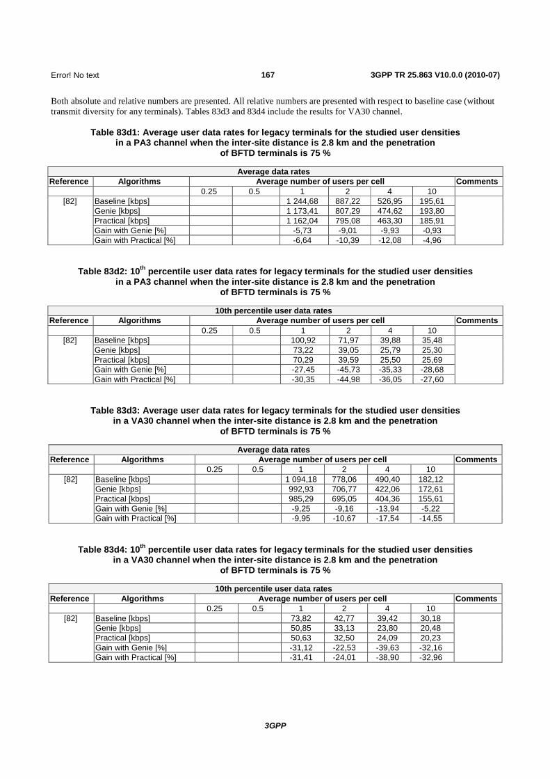
167
3GPP
Error! No text of specified
3GPP TR 25.863 V10.0.0 (2010-07)
Both absolute and relative numbers are presented. All relative numbers are presented with respect to baseline case (without transmit diversity for any terminals). Tables 83d3 and 83d4 include the results for VA30 channel.
Table 83d1: Average user data rates for legacy terminals for the studied user densities in a PA3 channel when the inter-site distance is 2.8 km and the penetration
of BFTD terminals is 75 %
Average data rates Reference Algorithms Average number of users per cell Comments
0.25 0.5 1 2 4 10 [82] Baseline [kbps] 1 244,68 887,22 526,95 195,61
Genie [kbps] 1 173,41 807,29 474,62 193,80 Practical [kbps] 1 162,04 795,08 463,30 185,91 Gain with Genie [%] -5,73 -9,01 -9,93 -0,93 Gain with Practical [%] -6,64 -10,39 -12,08 -4,96
Table 83d2: 10th percentile user data rates for legacy terminals for the studied user densities in a PA3 channel when the inter-site distance is 2.8 km and the penetration
of BFTD terminals is 75 %
10th percentile user data rates Reference Algorithms Average number of users per cell Comments
0.25 0.5 1 2 4 10 [82] Baseline [kbps] 100,92 71,97 39,88 35,48
Genie [kbps] 73,22 39,05 25,79 25,30 Practical [kbps] 70,29 39,59 25,50 25,69 Gain with Genie [%] -27,45 -45,73 -35,33 -28,68 Gain with Practical [%] -30,35 -44,98 -36,05 -27,60
Table 83d3: Average user data rates for legacy terminals for the studied user densities in a VA30 channel when the inter-site distance is 2.8 km and the penetration
of BFTD terminals is 75 %
Average data rates Reference Algorithms Average number of users per cell Comments
0.25 0.5 1 2 4 10 [82] Baseline [kbps] 1 094,18 778,06 490,40 182,12
Genie [kbps] 992,93 706,77 422,06 172,61 Practical [kbps] 985,29 695,05 404,36 155,61 Gain with Genie [%] -9,25 -9,16 -13,94 -5,22 Gain with Practical [%] -9,95 -10,67 -17,54 -14,55
Table 83d4: 10th percentile user data rates for legacy terminals for the studied user densities in a VA30 channel when the inter-site distance is 2.8 km and the penetration
of BFTD terminals is 75 %
10th percentile user data rates Reference Algorithms Average number of users per cell Comments
0.25 0.5 1 2 4 10 [82] Baseline [kbps] 73,82 42,77 39,42 30,18
Genie [kbps] 50,85 33,13 23,80 20,48 Practical [kbps] 50,63 32,50 24,09 20,23 Gain with Genie [%] -31,12 -22,53 -39,63 -32,16 Gain with Practical [%] -31,41 -24,01 -38,90 -32,96

168
3GPP
Error! No text of specified
3GPP TR 25.863 V10.0.0 (2010-07)
7.2.2 Bursty Traffic
7.2.2.1 Results for inter-site distance of 1km
7.2.2.1.1 Results for 0 dB long-term antenna imbalance and 2D antennas
Table 84, 84a, 84b and 84c presents the average user burst rates, the 10th percentile user burst rates and the average transmit power for the studied user densities in a PA3 channel with mean burst sizes of 125 KBytes, 30 KBytes, 5 KBytes and 1.25 KBytes respectively.
Table 84: Average user burst rates, 10th percentile user burst rates and average transmit power for the studied user densities in a PA3 channel when the inter-site distance is 1 km
with mean burst size 125 KBytes
Average user burst rate Reference Algorithms Average number of users per cell Comments
Penetration Loss [dB]
1 2 4 5 6
[76]
Baseline [Mbps]
10
6.09 5.39 4.04 3.29 Notes 1, 2 and 3
Practical [Mbps] 6.29 5.62 4.38 3.69 Gain with Practical [%]
3.13 4.25 8.36 12.28
[78]
Baseline [kbps]
10
1 071.07 1 070.25 1 072.72 1 041.11 Note 4 Note 5 Note 7
Practical [kbps] 1 074.03 1 073.29 1 076.74 1 061.97 Gain with Practical [%]
0.28 0.28 0.38 2.00
[76]
Baseline [Mbps]
20
4.67 4.20 3.25 2.72 Notes 1, 2 and 3
Practical [Mbps] 5.02 4.56 3.65 3.13 Gain with Practical [%]
7.54 8.60 12.27 15.16
[78]
Baseline [kbps]
20
1 037.3 1 028.1 1 011.2 964.23 Note 4 Note 5 Note 7
Practical [kbps] 1 049.0 1 043.0 1 033.0 1 009.5 Gain with Practical [%]
1.13 1.46 2.16 4.69
10th percentile user burst rates Reference Algorithms Average number of users per cell Comments
Penetration Loss [dB]
1 2 4 5 6
[76]
Baseline [Mbps]
10
4.85 4.33 3.15 2.40 Notes 1, 2 and 3
Practical [Mbps] 5.12 4.59 3.49 2.78 Gain with Practical [%]
5.47 5.91 10.74 15.60
[78]
Baseline [kbps]
10
996.03 996.39 998.31 959.63 Note 4 Note 5 Note 7
Practical [kbps] 1 000.99 1 000.42 1 003.51 985.46 Gain with Practical [%]
0.50 0.41 0.52 2.69
[76]
Baseline [Mbps]
20
1.31 1.09 0.80 0.66 Notes 1, 2 and 3
Practical [Mbps] 1.65 1.43 1.12 0.93 Gain with Practical [%]
26.22 32.02 39.88 41.34
[78]
Baseline [kbps]
20
955.4 939.2 874.8 654.76 Note 4 Note 5 Note 7
Practical [kbps] 974.3 968.0 956.5 898.4 Gain with Practical [%]
1.98 3.06 9.34 37.21

169
3GPP
Error! No text of specified
3GPP TR 25.863 V10.0.0 (2010-07)
Average transmit power (dBM) Reference Algorithms Average number of users per cell Comments
1 2 4 5 6
[76]
Baseline [dBm]
10
-17.26 -16.42 -14.86 -14.06 Notes 1, 2 and 3 Gain with
Practical[dB] 1.82 1.90 1.95 1.96
[78] Baseline [dBm]
10 -18.97 -18.42 -17.04 -15.07 Note 4
Note 5 Note 7
Gain with Practical[dB]
2.48 2.67 2.92 3.36
[76]
Baseline [dBm]
20
-7.56 -6.89 -5.62 -4.90 Notes 1, 2 and 3 Gain with
Practical[dB] 1.81 1.89 1.92 1.96
[78] Baseline [dBm]
20 -8.83 -8.23 -6.97 -5.08 Note 4
Note 5 Note 7
Gain with Practical[dB]
2.59 2.79 2.98 3.30
NOTE 1: Noise Rise Target = 7 dB. NOTE 2: Target 10 % BLER after 1st transmission with a maximum of 4 transmissions. NOTE 3: Note 3: NodeB Receiver: LMMSE Equalizer. NOTE 4: Target 1 % BLER after 4th transmission with a maximum of 4 transmissions. NOTE 5: NodeB Receiver: Rake. NOTE 6: Simulation assumes UE Category 7. NOTE 7: Simulation assumes UE Category 6.
Table 84a: Average user burst rates, 10th percentile user burst rates and average transmit power for the studied user densities in a PA3 channel when the inter-site distance is 1 km
with mean burst size 30 KBytes
Average user burst rate Reference Algorithms Average number of users per cell Comments
Penetration Loss [dB]
1 2 4 5 6
[78]
Baseline [kbps]
10
936.14 937.42 948.08 923.54 Note 4 Note 5 Note 7
Practical [kbps] 940.54 941.47 953.19 940.90 Gain with Practical [%]
0.47 0.43 0.54 1.88
[78]
Baseline [kbps]
20
912.25 906.94 897.45 854.38 Note 4 Note 5 Note 7
Practical [kbps] 921.75 918.37 916.24 895.19 Gain with Practical [%]
1.04 1.26 2.09 4.77
10th percentile user burst rates Reference Algorithms Average number of users per cell Comments
Penetration Loss [dB]
1 2 4 5 6
[78]
Baseline [kbps]
10
892.40 894.46 906.28 882.49 Note 4 Note 5 Note 7
Practical [kbps] 900.42 901.41 912.08 900.49 Gain with Practical [%]
0.90 0.78 0.64 2.04
[78]
Baseline [kbps]
20
879.22 874.94 827.26 608.12 Note 4 Note 5 Note 7
Practical [kbps] 890.31 889.34 892.24 854.31 Gain with Practical [%]
1.26 1.65 7.86 40.48

170
3GPP
Error! No text of specified
3GPP TR 25.863 V10.0.0 (2010-07)
Average transmit power (dBM) Reference Algorithms Average number of users per cell Comments
1 2 4 5 6
[78] Baseline [dBm]
10 -19.04 -18.50 -17.07 -15.04 Note 4
Note 5 Note 7
Gain with Practical[dB]
2.43 2.59 2.83 3.21
[78] Baseline [dBm]
20 -8.93 -8.34 -6.98 -5.05 Note 4
Note 5 Note 7
Gain with Practical[dB]
2.53 2.72 2.91 3.25
NOTE 1: Noise Rise Target = 7 dB. NOTE 2: Target 10 % BLER after 1st transmission with a maximum of 4 transmissions. NOTE 3: Note 3: NodeB Receiver: LMMSE Equalizer. NOTE 4: Target 1 % BLER after 4th transmission with a maximum of 4 transmissions. NOTE 5: NodeB Receiver: Rake. NOTE 6: Simulation assumes UE Category 7. NOTE 7: Simulation assumes UE Category 6.
Table 84b: Average user burst rates, 10th percentile user burst rates and average transmit power for the studied user densities in a PA3 channel when the inter-site distance is 1 km
with mean burst size 5 KBytes
Average user burst rate Reference Algorithms Average number of users per cell Comments
Penetration Loss [dB]
1 2 4 5 6
[78]
Baseline [kbps]
10
629.71 631.06 625.60 589.31 Note 4 Note 5 Note 7
Practical [kbps] 632.12 633.31 631.66 613.29 Gain with Practical [%]
0.38 0.36 0.97 4.07
[78]
Baseline [kbps]
20
617.32 614.97 594.40 545.24 Note 4 Note 5 Note 7
Practical [kbps] 621.89 620.07 608.45 583.06 Gain with Practical [%]
0.74 0.83 2.36 6.94
10th percentile user burst rates Reference Algorithms Average number of users per cell Comments
Penetration Loss [dB]
1 2 4 5 6
[78]
Baseline [kbps]
10
607.65 610.09 602.54 561.53 Note 4 Note 5 Note 7
Practical [kbps] 612.95 614.90 612.46 591.76 Gain with Practical [%]
0.87 0.79 1.65 5.38
[78]
Baseline [kbps]
20
603.59 603.86 574.42 438.15 Note 4 Note 5 Note 7
Practical [kbps] 609.62 609.59 599.87 554.24 Gain with Practical [%]
1.0 0.95 4.43 26.5
Average transmit power (dBM) Reference Algorithms Average number of users per cell Comments
1 2 4 5 6
[78] Baseline [dBm]
10 -18.82 -18.30 -16.75 -14.71 Note 4
Note 5 Note 7
Gain with Practical[dB]
2.19 2.33 2.50 2.89
[78] Baseline [dBm]
20 -8.73 -8.15 -6.70 -4.69 Note 4
Note 5 Note 7
Gain with Practical[dB]
2.31 2.48 2.63 2.95
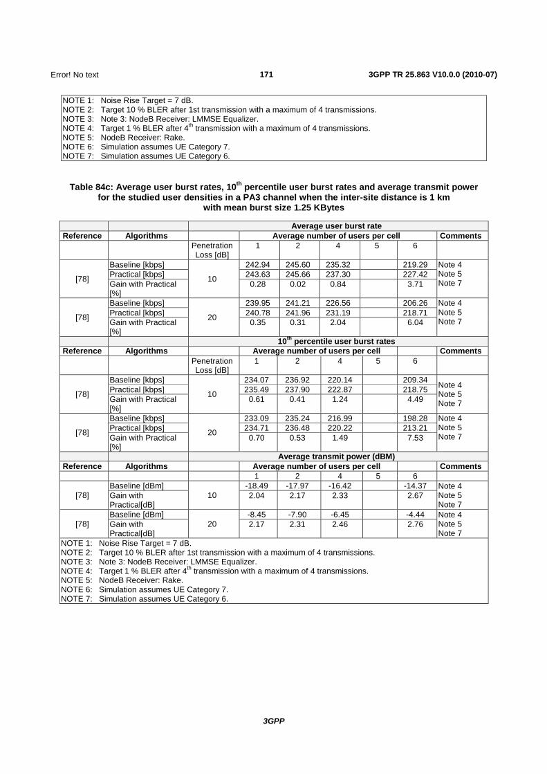
171
3GPP
Error! No text of specified
3GPP TR 25.863 V10.0.0 (2010-07)
NOTE 1: Noise Rise Target = 7 dB. NOTE 2: Target 10 % BLER after 1st transmission with a maximum of 4 transmissions. NOTE 3: Note 3: NodeB Receiver: LMMSE Equalizer. NOTE 4: Target 1 % BLER after 4th transmission with a maximum of 4 transmissions. NOTE 5: NodeB Receiver: Rake. NOTE 6: Simulation assumes UE Category 7. NOTE 7: Simulation assumes UE Category 6.
Table 84c: Average user burst rates, 10th percentile user burst rates and average transmit power for the studied user densities in a PA3 channel when the inter-site distance is 1 km
with mean burst size 1.25 KBytes
Average user burst rate Reference Algorithms Average number of users per cell Comments
Penetration Loss [dB]
1 2 4 5 6
[78]
Baseline [kbps]
10
242.94 245.60 235.32 219.29 Note 4 Note 5 Note 7
Practical [kbps] 243.63 245.66 237.30 227.42 Gain with Practical [%]
0.28 0.02 0.84 3.71
[78]
Baseline [kbps]
20
239.95 241.21 226.56 206.26 Note 4 Note 5 Note 7
Practical [kbps] 240.78 241.96 231.19 218.71 Gain with Practical [%]
0.35 0.31 2.04 6.04
10th percentile user burst rates Reference Algorithms Average number of users per cell Comments
Penetration Loss [dB]
1 2 4 5 6
[78]
Baseline [kbps]
10
234.07 236.92 220.14 209.34 Note 4 Note 5 Note 7
Practical [kbps] 235.49 237.90 222.87 218.75 Gain with Practical [%]
0.61 0.41 1.24 4.49
[78]
Baseline [kbps]
20
233.09 235.24 216.99 198.28 Note 4 Note 5 Note 7
Practical [kbps] 234.71 236.48 220.22 213.21 Gain with Practical [%]
0.70 0.53 1.49 7.53
Average transmit power (dBM) Reference Algorithms Average number of users per cell Comments
1 2 4 5 6
[78] Baseline [dBm]
10 -18.49 -17.97 -16.42 -14.37 Note 4
Note 5 Note 7
Gain with Practical[dB]
2.04 2.17 2.33 2.67
[78] Baseline [dBm]
20 -8.45 -7.90 -6.45 -4.44 Note 4
Note 5 Note 7
Gain with Practical[dB]
2.17 2.31 2.46 2.76
NOTE 1: Noise Rise Target = 7 dB. NOTE 2: Target 10 % BLER after 1st transmission with a maximum of 4 transmissions. NOTE 3: Note 3: NodeB Receiver: LMMSE Equalizer. NOTE 4: Target 1 % BLER after 4th transmission with a maximum of 4 transmissions. NOTE 5: NodeB Receiver: Rake. NOTE 6: Simulation assumes UE Category 7. NOTE 7: Simulation assumes UE Category 6.

172
3GPP
Error! No text of specified
3GPP TR 25.863 V10.0.0 (2010-07)
Tables 85, 85a, 85b and 85c presents the average user burst rates, the 10th percentile user burst rates and the average transmit power for the studied user densities in a VA30 channel with mean burst sizes of 125 KBytes, 30 KBytes, 5 KBytes and 1.25 KBytes respectively.
Table 85: Average user burst rates, 10th percentile user burst rates and average transmit power for the studied user densities in a VA30 channel when the inter-site distance is 1 km
with mean burst size 125 KBytes
Average user burst rate Reference Algorithms Average number of users per cell Comments
Penetration Loss [dB]
1 2 4 5 6
[76]
Baseline [Mbps]
10
4.59 3.96 2.55 1.53 Notes 1, 2 and 3
Practical [Mbps] 4.67 4.06 2.71 1.68 Gain with Practical [%]
1.68 2.47 6.10 9.80
[78]
Baseline [kbps]
10
1 151.0 1 150.5 1 131.8 1 020.7 Note 4 Note 5 Note 7
Practical [kbps] 1 139.7 1 139.2 1 123.4 1 023.2 Gain with Practical [%]
-0.98 -0.98 -0.74 0.25
[76]
Baseline [Mbps]
20
3.65 3.17 2.10 1.44 Notes 1, 2 and 3
Practical [Mbps] 3.78 3.31 2.25 1.63 Gain with Practical [%]
3.49 4.5 7.20 13.24
[78]
Baseline [kbps]
20
1 095.0 1 083.5 1 047.9 950.82 Note 4 Note 5 Note 7
Practical [kbps] 1 090.5 1 079.6 1 047.8 959.73 Gain with Practical [%]
-0.41 -0.37 -0.0 0.94
10th percentile user burst rates Reference Algorithms Average number of users per cell Comments
Penetration Loss [dB]
1 2 4 5 6
[76]
Baseline [Mbps]
10
3.82 3.23 1.84 0.79 Notes 1, 2 and 3
Practical [Mbps] 3.82 3.32 1.99 1.04 Gain with Practical [%]
0.00 2.58 8.14 30.50
[78]
Baseline [kbps]
10
1 081.4 1 081.8 1 056.8 886.5, Note 4 Note 5 Note 7
Practical [kbps] 1 073.4 1 070.6 1 049.2 898.2 Gain with Practical [%]
-0.74 -1.03 -0.71 1.32
[76]
Baseline [Mbps]
20
0.98 0.69 0.41 0.25 Notes 1, 2 and 3
Practical [Mbps] 1.17 0.83 0.50 0.34 Gain with Practical [%]
19.30 20.43 22.16 32.44
[78]
Baseline [kbps]
20
996.9 937.1 752.2 537.06 Note 4 Note 5 Note 7
Practical [kbps] 1 002.6 964.5 818.1 585.08 Gain with Practical [%]
0.58 2.92 8.77 8.94

173
3GPP
Error! No text of specified
3GPP TR 25.863 V10.0.0 (2010-07)
Average transmit power (dBM) Reference Algorithms Average number of users per cell Comments
1 2 4 5 6
[76] Baseline [dBm]
10 -16.92 -15.87 -13.90 -12.67 Notes 1, 2
and 3 Gain with Practical[dB]
0.59 0.64 0.68 0.76
[78] Baseline [dBm]
10 -19.07 -18.44 -16.73 -14.68 Note 4
Note 5 Note 7
Gain with Practical[dB]
0.54 0.58 0.60 0.62
[76]
Baseline [dBm]
20
-7.21 -6.23 -4.54 -3.59 Notes 1, 2 and 3 Gain with
Practical[dB] 0.60 0.66 0.68 0.74
[78] Baseline [dBm]
20 -9.13 -8.49 -6.98 -5.07 Note 4
Note 5 Note 7
Gain with Practical[dB]
0.56 0.62 0.61 0.65
NOTE 1: Noise Rise Target = 7 dB. NOTE 2: Target 10 % BLER after 1st transmission with a maximum of 4 transmissions. NOTE 3: Note 3: NodeB Receiver: LMMSE Equalizer. NOTE 4: Target 1 % BLER after 4th transmission with a maximum of 4 transmissions. NOTE 5: NodeB Receiver: Rake. NOTE 6: Simulation assumes UE Category 7. NOTE 7: Simulation assumes UE Category 6.
Table 85a: Average user burst rates, 10th percentile user burst rates and average transmit power for the studied user densities in a VA30 channel when the inter-site distance is 1 km
with mean burst size 30 KBytes
Average user burst rate Reference Algorithms Average number of users per cell Comments
Penetration Loss [dB]
1 2 4 5 6
[78]
Baseline [kbps]
10
997.75 999.59 982.26 876.69 Note 4 Note 5 Note 7
Practical [kbps] 986.84 988.63 974.6 880.36 Gain with Practical [%]
-1.09 -1.10 -0.78 0.42
[78]
Baseline [kbps]
20
954.59 947.01 912.31 816.28 Note 4 Note 5 Note 7
Practical [kbps] 948.57 942.13 911.81 822.41 Gain with Practical [%]
-0.59 -0.52 -0.05 0.75
10th percentile user burst rates Reference Algorithms Average number of users per cell Comments
Penetration Loss [dB]
1 2 4 5 6
[78]
Baseline [kbps]
10
963.64 966.59 946.48 786.78 Note 4 Note 5 Note 7
Practical [kbps] 954.22 955.59 938.85 797.22 Gain with Practical [%]
-0.98 -1.14 -0.81 1.33
[78]
Baseline [kbps]
20
921.82 874.39 696.36 465.71 Note 4 Note 5 Note 7
Practical [kbps] 920.78 901.98 755.14 528.65 Gain with Practical [%]
0.11 3.15 8.44 13.51
Average transmit power (dBM) Reference Algorithms Average number of users per cell Comments
1 2 4 5 6
[78] Baseline [dBm]
10 -19.30 -18.67 -16.91 -14.73 Note 4
Note 5 Note 7
Gain with Practical[dB]
0.53 0.57 0.58 0.62
[78] Baseline [dBm] 20 -9.35 -8.70 -7.10 -5.07 Note 4 Note 5 Gain with 0.55 0.61 0.60 0.57

174
3GPP
Error! No text of specified
3GPP TR 25.863 V10.0.0 (2010-07)
Practical[dB] Note 7 NOTE 1: Noise Rise Target = 7 dB. NOTE 2: Target 10 % BLER after 1st transmission with a maximum of 4 transmissions. NOTE 3: Note 3: NodeB Receiver: LMMSE Equalizer. NOTE 4: Target 1 % BLER after 4th transmission with a maximum of 4 transmissions. NOTE 5: NodeB Receiver: Rake. NOTE 6: Simulation assumes UE Category 7. NOTE 7: Simulation assumes UE Category 6.
Table 85b: Average user burst rates, 10th percentile user burst rates and average transmit power for the studied user densities in a VA30 channel when the inter-site distance is 1 km
with mean burst size 5 KBytes
Average user burst rate Reference Algorithms Average number of users per cell Comments
Penetration Loss [dB]
1 2 4 5 6
[78]
Baseline [kbps]
10
645.41 648.89 627.52 529.72 Note 4 Note 5 Note 7
Practical [kbps] 639.63 643.15 623.74 535.40 Gain with Practical [%]
-0.90 -0.86 -0.60 1.07
[78]
Baseline [kbps]
20
622.72 620.89 587.85 507.63 Note 4 Note 5 Note 7
Practical [kbps] 619.60 618.14 588.09 508.44 Gain with Practical [%]
-0.50 -0.44 0.04 0.16
10th percentile user burst rates Reference Algorithms Average number of users per cell Comments
Penetration Loss [dB]
1 2 4 5 6
[78]
Baseline [kbps]
10
630.0, 633.10 603.14 471.0, Note 4 Note 5 Note 7
Practical [kbps] 624.66 628.38 599.59 479.86 Gain with Practical [%]
-0.85 -0.75 -0.59 1.88
[78]
Baseline [kbps]
20
614.41 602.07 502.55 354.41 Note 4 Note 5 Note 7
Practical [kbps] 611.09 607.80 528.87 366.62 Gain with Practical [%]
-0.54 0.95 5.24 3.44
Average transmit power (dBM) Reference Algorithms Average number of users per cell Comments
1 2 4 5 6
[78] Baseline [dBm]
10 -19.36 -18.76 -16.90 -14.69 Note 4
Note 5 Note 7
Gain with Practical[dB] 0.50 0.53 0.54 0.58
[78] Baseline [dBm]
20 -9.43 -8.80 -7.10 -5.2 Note 4
Note 5 Note 7
Gain with Practical[dB] 0.52 0.57 0.55 0.43
NOTE 1: Noise Rise Target = 7 dB. NOTE 2: Target 10 % BLER after 1st transmission with a maximum of 4 transmissions. NOTE 3: Note 3: NodeB Receiver: LMMSE Equalizer. NOTE 4: Target 1 % BLER after 4th transmission with a maximum of 4 transmissions. NOTE 5: NodeB Receiver: Rake. NOTE 6: Simulation assumes UE Category 7. NOTE 7: Simulation assumes UE Category 6.
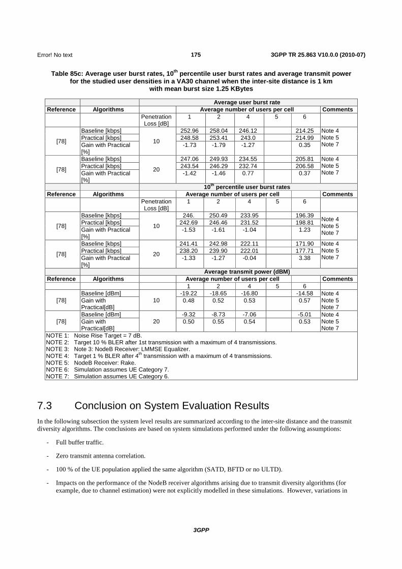
175
3GPP
Error! No text of specified
3GPP TR 25.863 V10.0.0 (2010-07)
Table 85c: Average user burst rates, 10th percentile user burst rates and average transmit power for the studied user densities in a VA30 channel when the inter-site distance is 1 km
with mean burst size 1.25 KBytes
Average user burst rate Reference Algorithms Average number of users per cell Comments
Penetration Loss [dB]
1 2 4 5 6
[78]
Baseline [kbps]
10
252.96 258.04 246.12 214.25 Note 4 Note 5 Note 7
Practical [kbps] 248.58 253.41 243.0 214.99 Gain with Practical [%]
-1.73 -1.79 -1.27 0.35
[78]
Baseline [kbps]
20
247.06 249.93 234.55 205.81 Note 4 Note 5 Note 7
Practical [kbps] 243.54 246.29 232.74 206.58 Gain with Practical [%]
-1.42 -1.46 0.77 0.37
10th percentile user burst rates Reference Algorithms Average number of users per cell Comments
Penetration Loss [dB]
1 2 4 5 6
[78]
Baseline [kbps]
10
246. 250.49 233.95 196.39 Note 4 Note 5 Note 7
Practical [kbps] 242.69 246.46 231.52 198.81 Gain with Practical [%]
-1.53 -1.61 -1.04 1.23
[78]
Baseline [kbps]
20
241.41 242.98 222.11 171.90 Note 4 Note 5 Note 7
Practical [kbps] 238.20 239.90 222.01 177.71 Gain with Practical [%]
-1.33 -1.27 -0.04 3.38
Average transmit power (dBM) Reference Algorithms Average number of users per cell Comments
1 2 4 5 6
[78] Baseline [dBm]
10 -19.22 -18.65 -16.80 -14.58 Note 4
Note 5 Note 7
Gain with Practical[dB]
0.48 0.52 0.53 0.57
[78] Baseline [dBm]
20 -9.32 -8.73 -7.06 -5.01 Note 4
Note 5 Note 7
Gain with Practical[dB]
0.50 0.55 0.54 0.53
NOTE 1: Noise Rise Target = 7 dB. NOTE 2: Target 10 % BLER after 1st transmission with a maximum of 4 transmissions. NOTE 3: Note 3: NodeB Receiver: LMMSE Equalizer. NOTE 4: Target 1 % BLER after 4th transmission with a maximum of 4 transmissions. NOTE 5: NodeB Receiver: Rake. NOTE 6: Simulation assumes UE Category 7. NOTE 7: Simulation assumes UE Category 6.
7.3 Conclusion on System Evaluation Results In the following subsection the system level results are summarized according to the inter-site distance and the transmit diversity algorithms. The conclusions are based on system simulations performed under the following assumptions:
- Full buffer traffic.
- Zero transmit antenna correlation.
- 100 % of the UE population applied the same algorithm (SATD, BFTD or no ULTD).
- Impacts on the performance of the NodeB receiver algorithms arising due to transmit diversity algorithms (for example, due to channel estimation) were not explicitly modelled in these simulations. However, variations in

176
3GPP
Error! No text of specified
3GPP TR 25.863 V10.0.0 (2010-07)
received signal levels or the DPCCH set point due to the transmit diversity algorithms are implicitly captured in the simulations.
- The uplink power control algorithm (at NodeB) is based on a SIR target comparison where an UP (DOWN) command is always assumed to be sent if the measured SIR is below (above) the SIR target.
- Some of the simulations used ideal signal to interference ratio (SIR) estimation at the NodeB.
- The indoor-to-outdoor penetration was modelled by a constant 10 dB loss which was applied to all the UE's.
- Antenna efficiencies and other antenna impairments, including variations of antenna gain for different angles of departure have been incorporated by the short-term and long term antenna imbalance. See section 5.3.1.
7.3.1 Switched antenna diversity
7.3.1.1 Inter-site distance 1 km
For a slow fading low dispersive channel (PedA 3 kmph), the gains in the average and 10th percentile user throughputs ranged between 2 % and 10 %. When one considered 3D antenna patterns, the gains were somewhat lower (see table 43). The UE transmit power reduction was around 1 dB.
For a faster fading and more dispersive channel (VehA 30 kmph), there were no significant gains or losses in average and 10th percentile user throughputs. The UE transmit power reduction was around 0.5 dB.
When the long term antenna imbalance was -4 dB, the user throughput gains were negligible for both types of channels and the UE transmit power was higher (see tables 45 to 47).
7.3.1.2 Inter-site distance 2.8 km
For a slow fading low dispersive channel (PedA 3 kmph), the gains in the average throughput was around 5 %. For the 10th percentile user throughputs, the gains in this scenario were inconsistent amongst companies (see table 49) and were in the range of 10 % to 40 %. A possible reason for this variation could be different MAC-e scheduler designs. In addition, some companies noted that they did not consider PA3 to be a representative channel for users near the edge of a 2.8 km cell due to its low level of dispersion. The UE transmit power reduction was between 0.5 dB and 2 dB.
For a faster fading and more dispersive channel (VehA 30 kmph), the gains in the average throughput were less than 4 %. For the 10th percentile user throughputs, the gains ranged from 0 % to 20 % and were again inconsistent amongst companies. The UE transmit power reduction was between 0 dB and 0.5 dB.
From the above observations, it is seen that at least for some MAC-e scheduler designs, switched antenna transmit diversity could offer gains in cell-edge throughput in both slow and fast fading channels under this scenario.
7.3.2 Beam forming antenna diversity
7.3.2.1 Inter-site distance 1 km
For a slow fading low dispersive channel (PedA 3 kmph), the gains in the average and 10th percentile user throughputs ranged between 4 % and 20 %. When one considered 3D antenna patterns, the gains were somewhat lower (see table 65). The UE transmit power reduction was around 1.5 dB.
For a faster fading and more dispersive channel (VehA 30 kmph), there were no significant gains or losses in average and 10th percentile user throughputs. The UE transmit power reduction was around 0.5 dB.
When the long term antenna imbalance was -4 dB, the user throughput gains were negligible for both types of channels and the UE transmit power was higher (see tables 67 and 68).

177
3GPP
Error! No text of specified
3GPP TR 25.863 V10.0.0 (2010-07)
7.3.2.2 Inter-site distance 2.8 km
For a slow fading low dispersive channel (PedA 3 kmph), the gains in the average throughput ranged between 5 % and 20 %. For the 10th percentile user throughputs, the gains in this scenario were inconsistent amongst companies (see table 62) and were in the range of 10 % to 60 %. A possible reason for this variation could be different MAC-e scheduler designs. In addition, some companies noted that they did not consider PA3 to be a representative channel for users near the edge of a 2.8 km cell due to its low level of dispersion. The UE transmit power reduction was between 0.5 dB and 2.5 dB.
For a faster fading and more dispersive channel (VehA 30 kmph), the gains in the average throughput were less than 3 %. For the 10th percentile user throughputs, gains up to 20 % were observed but were again inconsistent amongst companies. For some MAC-e scheduler designs, zero gains or small losses were seen (see table 75) with zero Tx antenna correlation. The UE transmit power reduction was between 0 dB and 0.6 dB.
From the above observations, it is seen that at least for some MAC-e scheduler designs, beamforming transmit diversity could offer gains in cell-edge throughput in both slow and fast fading channels under this scenario.
8 Impacts on UE Implementation
8.1 Switched Antenna Transmit Diversity In figure 32, a block diagram of a single band capable SATD UE transmitter is shown. As seen in figure 32, the transmit chain is identical to a legacy UE that transmits on a single antenna only, until the output of the Power Amplifier (PA).
The SATD UE differs from a non-ULTD legacy UE as follows:
- Antenna Selection Logic to decide which transmit antenna the UE should transmit on. One example of this logic is described in section 4.3.1, wherein the logic to decide to switch or not is based on accumulated TPC commands fed back from the NodeB to the UE. In the studies presented in the report, this nominal rate at which this logic can be executed is once per radio frame.
- Additional duplexer for the 2nd transmit antenna.
- 2nd transmit antenna1.
- RF Switch to switch between one of the duplexer/antennas.
1 If the non-ULTD legacy UE supports Rx diversity, there is no need to have an additional 2nd transmit antenna.

178
3GPP
Error! No text of specified
3GPP TR 25.863 V10.0.0 (2010-07)
å
Figure 32: Block Diagram of SATD transmitter
8.2 Beamforming Transmit Diversity In figures 33 and 34, a block diagram of a single band capable BFTD UE transmitter is shown. As seen in figure 33, the transmit chain is identical to a legacy UE that transmits on a single antenna only, until the output of the modulation block. It should be noted that to ensure that there is no impact to the PRACH coverage at least one of the two PAs would need to be of full power. With respect to Figure 34 it should also be noted that this report has only studied algorithms in which
21=a . To support beamforming algorithm where a is allowed to vary between 0 and 1 may require two full power PAs.
å
Figure 33: Block Diagram of BFTD transmitter

179
3GPP
Error! No text of specified
3GPP TR 25.863 V10.0.0 (2010-07)
21 a-
a jje-
jje
Figure 34: Beamforming Logic based on a symmetric implementation of a beam forming algortihm
The BFTD UE differs from a non-ULTD legacy UE as follows:
- Introduction of a beamforming block at the output of the modulation block.
· Note that the beamforming block could be implemented in digital base-band and performed prior to RF modulation. In that case, there may be a need to introduce an additional Digital to Analogue converter (DAC).
- There are 2 aspects to the beamforming block:
· Selection of beamforming weights: An example of the logic based on processing TPC commands fed back from the NodeB to the UE can be found in the reference beamforming algorithm described in section 4.3.2. The nominal rate at which the logic is executed is once every radio slot (0.667 ms).
· Application of beamforming weights: The details of the processing involved are shown in figure 3 for the case of asymmetric beamforming. In the most general case, the UE applies an amplitude and a phase offset between the two transmit paths. Note that with reference to the logic in figure 3, an additional complex multiplier would be needed for the case of symmetric beamforming.
- The amplitude and phase offset may belong to a finite quantized set.
- Note that in order to avoid implementing two full power PAs a would need to be restricted. Even in this case however BFTD UEs would need to have one full power PA so that they can perform PRACH according to legacy procedures.
- Additional power amplifier (PA).
· This in turn requires an additional PA calibration procedure.
- Additional duplexer for the 2nd transmit antenna.
- 2nd transmit antenna2.
2 If the non-ULTD legacy UE supports Rx diversity, there is no need to have an additional 2nd transmit antenna.

180
3GPP
Error! No text of specified
3GPP TR 25.863 V10.0.0 (2010-07)
8.2.1 UE Implementation Impact to maintain PRACH Coverage In the case when a BFTD capable UE has at least one full-power PA, in Idle and CELL_FACH state, the UE could perform legacy RACH procedures as defined today without enabling BFTD. However even in this case, it may still be possible to operate as if the BFTD UE utilizes two half power PAs in CELL_DCH. For example, in figure 35, the BFTD UE uses a full-power PA for the primary transmit antenna and a half-power PA for the diversity transmit antenna. During regular data transmission in CELL_DCH, when BFTD is enabled, the UE changes the primary full-power PA's supply voltage using the technique of dynamic voltage scaling or average power tracking to improve its efficiency at mid-to-high Tx power, effectively approximating a half-power PA's efficiency performance. It should however be noted that in order to avoid potential performance degradations associated with PRACH coverage it would be necessary to require (and test) that BFTD capable UEs only transmit from one antenna in other states than CELL_DCH.
Figure 35: BFTD with Average Power Tracking (APT) Power Amplifiers
8.3 Summary of UE Implementation Impact due to ULTD The impact to the UE implementation due to UL Transmit Diversity in HSPA can be summarized in table 86 for both SATD and BFTD UEs.
Table 86: Summary of UE Implementation Impact
Baseline non-ULTD UE
SATD UE BFTD UE
ULTD Control or Decision Logic N/A Antenna selection algorithm to select transmit antenna.
Beamforming weight selection algorithm to select relative
Amplitude and phase between the pair of antennas
Additional ULTD related logic RF switch to switch between the two
antennas
2 real multipliers (second antenna amplitude)
2 complex multiplier and LUT† (second antenna, phase)
Number of DACs 1 1 2‡ Number of Power Amplifiers 1 1 2 Number of Duplexers 1 2 2 Number of Transmit Antennas 1 2 2
NOTE: If the non-ULTD legacy UE supports Rx diversity, there is no need to have an additional 2nd transmit antenna.
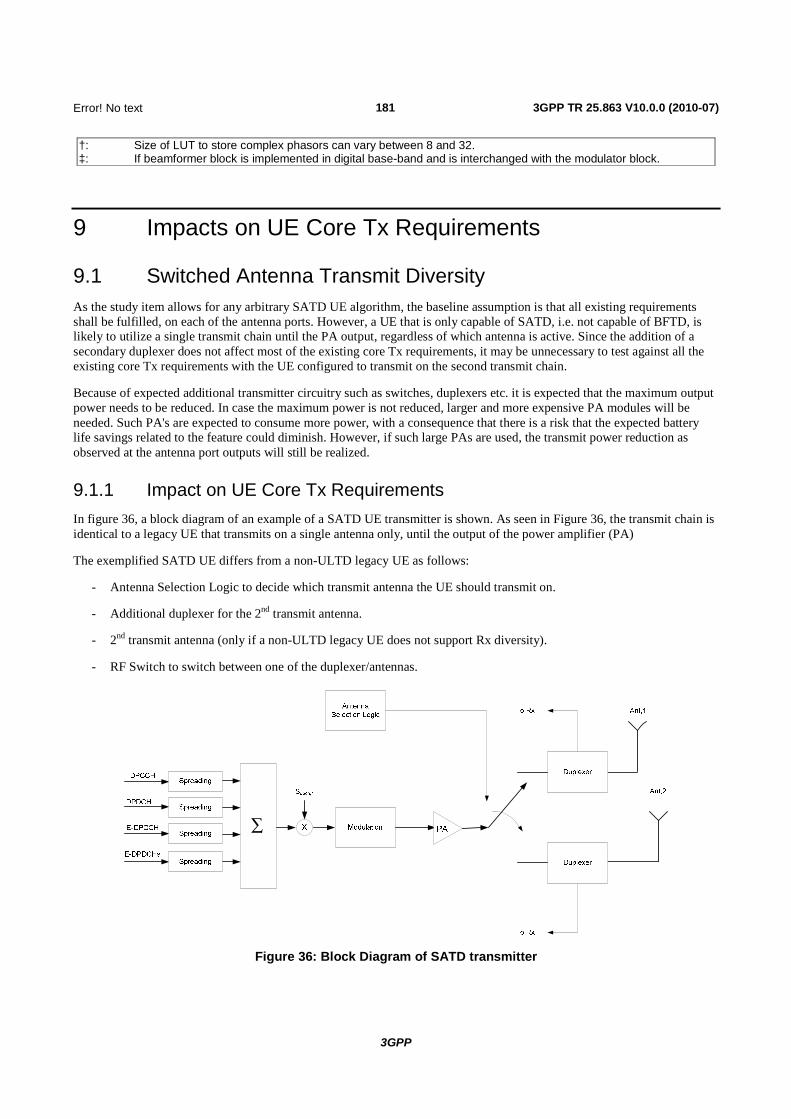
181
3GPP
Error! No text of specified
3GPP TR 25.863 V10.0.0 (2010-07)
†: Size of LUT to store complex phasors can vary between 8 and 32. ‡: If beamformer block is implemented in digital base-band and is interchanged with the modulator block.
9 Impacts on UE Core Tx Requirements
9.1 Switched Antenna Transmit Diversity As the study item allows for any arbitrary SATD UE algorithm, the baseline assumption is that all existing requirements shall be fulfilled, on each of the antenna ports. However, a UE that is only capable of SATD, i.e. not capable of BFTD, is likely to utilize a single transmit chain until the PA output, regardless of which antenna is active. Since the addition of a secondary duplexer does not affect most of the existing core Tx requirements, it may be unnecessary to test against all the existing core Tx requirements with the UE configured to transmit on the second transmit chain.
Because of expected additional transmitter circuitry such as switches, duplexers etc. it is expected that the maximum output power needs to be reduced. In case the maximum power is not reduced, larger and more expensive PA modules will be needed. Such PA's are expected to consume more power, with a consequence that there is a risk that the expected battery life savings related to the feature could diminish. However, if such large PAs are used, the transmit power reduction as observed at the antenna port outputs will still be realized.
9.1.1 Impact on UE Core Tx Requirements In figure 36, a block diagram of an example of a SATD UE transmitter is shown. As seen in Figure 36, the transmit chain is identical to a legacy UE that transmits on a single antenna only, until the output of the power amplifier (PA)
The exemplified SATD UE differs from a non-ULTD legacy UE as follows:
- Antenna Selection Logic to decide which transmit antenna the UE should transmit on.
- Additional duplexer for the 2nd transmit antenna.
- 2nd transmit antenna (only if a non-ULTD legacy UE does not support Rx diversity).
- RF Switch to switch between one of the duplexer/antennas.
å
Figure 36: Block Diagram of SATD transmitter

182
3GPP
Error! No text of specified
3GPP TR 25.863 V10.0.0 (2010-07)
Considering the similarity of the two Tx chains as shown in figure 36, the difference between the two Tx chains is due to the different duplexers and different paths inside the switch. Since the different paths inside the switch can be assumed negligible, we can assume that the duplexer is a main source of difference. Since a UE that is only capable of SATD, utilizes a single, common, transmit chain until the PA output and the duplexer does not affect most of existing core Tx requirements, there is no need to test against all core Tx requirements again with the second transmit chain when the UE is operating in SATD mode.
When we restrict the applicability of SATD tests to only single carrier operation on the uplink, the following test methodology is proposed:
- Perform core UE transmitter tests as currently defined in 3GPP TS 25.101 on the primary antenna:
· Due to the insertion of additional switch for SATD as shown in figure 36 in the UL Tx chain, there might be some impact on maximum UL transmit power. In order to maintain the same PA size, we may need to reduce the maximum UL transmit power by the amount of additional insertion loss due to the switch.
- Perform only the following core UE transmitter tests as currently defined in 25.101 on the secondary or diversity antenna:
· UE maximum output power (6.2.1).
· Spurious Emissions (6.6.3).
· Error Vector Magnitude (6.8.2).
The motivation here is to test only those UE transmitter characteristics that might differ due to a mismatch in the duplexer filter responses. In addition, to ensure that the UE operating an SATD will not cause any detrimental effects to overall system performance, new core Tx requirements are recommended in section 10.1.
9.1.2 Impact on UE Core Rx Requirements Due to the SATD operation, at any given time, the UE could transmit through one of the duplexer/antenna pairs. As a result, it may be useful to additionally verify that the UE meets the REFSENS requirement using the diversity receive path when the UE transmits with maximum output power on each diversity transmit path of the duplexer/antenna pairs. The main purpose of this test is to verify the duplexer isolation in the diversity chain. A suitable test methodology is as follows:
- Perform UE Rx core tests as currently defined in 3GPP TS 25.101 by configuring the UE to transmit on the primary transmit antenna.
- Perform the REFSENS test with the diversity receive path by configuring the UE to transmit on the secondary or diversity transmit antenna.
9.2 Beamforming Transmit Diversity Provide impacts on UE core Tx requirements due to the practical algorithm(s) considered in this study for beamforming transmit diversity.
10 New UE Core Tx Requirements
10.1 Test Feasibility It may be difficult by way of a RAN4 test requirement to fully ensure that the UE transmit diversity algorithms do not degrade system performance. For this purpose, higher layer signaling to enable/disable the uplink transmit diversity transmission could be considered as a possible method to mitigate some of these concerns that cannot be addressed with RAN4 testing or performance requirements.

183
3GPP
Error! No text of specified
3GPP TR 25.863 V10.0.0 (2010-07)
10.2 Switched Antenna Transmit Diversity
10.2.1 Antenna Switching Rate Based on the link and system study of the genie algorithm as described in section 4.2.1 and the practical SATD algorithm as described in section 4.3.1, a new transmit core requirement for SATD devices can be considered that should limit the transmit antenna switching rate in terms of the number of antenna switches per second for corresponding algorithms. The purpose of introducing such a limit on the antenna switching rate is to upper bound the potential impact that could be caused at the NodeB receiver (for example channel estimation, etc.).
The additional Tx core requirement to test for the antenna switching rate could be verified with a test setup as shown in figure 37. Since the criteria which the UE rely on when deciding whether or not to switch antenna is unknown (TPC commands represents one out of many possible criteria). Note that it could be challenging to design a test that can ensure that a particular SATD algorithm complies with this requirement.
Figure 37: Testing Antenna Switching Rate in SATD devices
At a high level, the test setup can be summarized as follows:
- System Simulator (SS) sets up a call with the UE.
- Once the UE is in CELL_DCH, SS sends a dummy pattern of TPC bits to UE:
· The choice of dummy TPC pattern is TBD and can be determined based on collecting traces of TPC bits from a link simulation.
- SS detects when an antenna switch happens by sensing the absence or presence of a signal at it's receiver:
· UE should be transmitting at a sufficiently high power to allow for the SS to detect its absence.
· When the UE switches to the secondary or diversity antenna, there is no connection with the SS receiver.
10.3 Beamforming Transmit Diversity Provide new UE core Tx requirements for the practical algorithm(s) considered in this study for beamforming transmit diversity. New requirements will be defined to ensure the UE with beamforming transmit diversity will not cause any detrimental effects to overall system performance.

184
3GPP
Error! No text of specified
3GPP TR 25.863 V10.0.0 (2010-07)
11 Analysis of UE Battery Life and Heat Reduction Savings due to ULTD
In this section, an analysis of UE battery life and heat reduction savings due to ULTD is provided. The analysis is performed based on two different methodologies:
- Method 1: In this method [72], [73], using the PA efficiency characteristic and UE transmit power profiles (Voice and Data) as input, the UE battery life savings and heat reduction was obtained as a function of different UE transmit power reduction values. The analysis, based on this method was performed for both SATD and BFTD.
- Method 2: In this method [74], using the PA efficiency characteristic as input, the average UE battery life savings is computed, based on the probability distribution of the UE transmit powers as observed in a system simulation when ULTD is enabled. The analysis, based on this method was performed only for SATD.
11.1 Method 1
11.1.1 PA Efficiency Curves Figure 37 shows the efficiency characteristic of a PA with dynamic voltage scaling used in the analysis. As seen in the figure, the efficiency ranges from ~0 % to 40 % as the UE transmit power varies from -8 dBm to 24 dBm. A 40 % efficiency at a PA transmit power of 24 dBm results in an output power of 630 mW and 945 mW is transformed into heat. Figures 38 and 39 show the efficiency characteristic of a full-power PA and a half-power PA with 3 gain states respectively [72]. It should be noted that different UE manufacturers tend to use different PA:s and that the conclusions thus might change depending on which of the PA characteristics used. As can be seen the efficiency for a PA employing dynamic voltage scaling is significantly higher at medium to high output powers. Hence it is reasonable to expect that data-centric devices primarily would employ PA:s based on dynamic voltage scaling. For SATD, one full-power PA will be assumed. For BFTD two architectures are studied. In the first one full-power PA for the primary transmit chain and one half-power PA for the secondary transmit chain will be assumed and in the second two half-power PAs are assumed. It should however be mentioned that an architecture with two half-power PAs may not be viable since it is likely to degrade the PRACH performance.
0.0%
5.0%
10.0%
15.0%
20.0%
25.0%
30.0%
35.0%
40.0%
45.0%
-10 -5 0 5 10 15 20 25 30
Pow
er A
dded
Effi
cienc
y
Tx Power (dBm)
PA Efficiency with Dynamic Voltage Scaling
Figure 37: PA Efficiency with Dynamic Voltage Scaling (DVS) or Average Power Tracking (APT) [69]

185
3GPP
Error! No text of specified
3GPP TR 25.863 V10.0.0 (2010-07)
Figure 38: Full-Power PA Efficiency with 3 Gain States [72]
Figure 39: Half-Power PA Efficiency with 3 Gain States [72]
11.1.2 UE Transmit Power Profiles In the analysis performed in Method 1, two UE transmit power profiles were used:

186
3GPP
Error! No text of specified
3GPP TR 25.863 V10.0.0 (2010-07)
- The CDG35 user transmit power profile derived in [70] and plotted in figure 40.
- A power profile captured from a live network from a single user with a Rel-6 UE transmitting full buffer traffic from a single position (figure 41). This profile is intended as one demonstrative example of UEs carrying out HSUPA data transmission close to cell edge. It is recognized that the results related with this power profile may not be used for drawing general conclusions regarding potential power savings.
0.00%0.50%1.00%1.50%2.00%2.50%3.00%3.50%4.00%4.50%
2319151173-1-5-9-13-17-21-25-29-33-37-41-45-49
RF Output Power at Antenna [dBm]
Figure 40: PDF of transmit power for CDG suburban profile (Mean = 10.6 dBm, Standard Deviation = 15.6 dBm)
Figure 41: PDF of transmit power for one stationary user location in a certain network deployment with a HSUPA Stationary Full-Buffer traffic model

187
3GPP
Error! No text of specified
3GPP TR 25.863 V10.0.0 (2010-07)
11.1.3 UE Transmit Architecture Assumption for BFTD Two PA architectures for the BFTD, shown in Figure 42 (using one full-power and one ½ power PA) and figure 43 (using two ½ power Pas) are analyzed. While the BFTD UE with two ½ power PAs can operate more efficiently, it may degrade PRACH performance., The BFTD UE with a full power PA ( and a ½ power PA) are capable of working like a regular UE in the case BFTD is turned off.
Ant 1
Ant 2BasebandProcessor
ULTDTransceiver
Duplexer
Duplexer
Full Power PA
Half Power PA
Controlsignal
Baseband Tx signal
Figure 42: BFTD with Full/Half Power Amplifier
BasebandProcessor
ULTDTransceiver
Duplexer
Duplexer
Half Power PA
Half Power PA
Controlsignal
Baseband Tx signal
Ant 1
Ant 2
Figure 43: BFTD with Dual Half Power Amplifier. This architecture may suffer degraded RACH performance and is less viable to use in practice
11.2 Method 2 When computing the PA-related battery savings due to SATD, the following methodology was adopted:
- A PA efficiency curve (figure 37) and a probability density function of the UE transmit power are used as input parameters. The probability distribution function of the UE transmit power (at the input to the antenna(s)) has been collected via system simulations and it is dependent on the specific scenario (inter-site distance, channel type, uplink transmit diversity algorithm, etc.).
- Based on the PA efficiency curve, we compute the power that is consumed by the PA and the switch given a certain transmit power (figure 44). This relationship can be expressed as

188
3GPP
Error! No text of specified
3GPP TR 25.863 V10.0.0 (2010-07)
tx
eff
L
input ppinsertion
h
1010= (1)
where insertionL is the insertion loss associated with the switch, effh is the PA efficiency, inputp
the power before the switch
and txp the UE transmit power.
- Given the probability density function of the UE transmit power the expected PA power consumption (before the switch) pinput can be computed. For the sake of clarity, we highlight that this computation is performed in linear domain.
Using the above described 3-step approach the expected power consumed by the different algorithms for different loads and channel types can be readily obtained. All the results are presented as a function of the insertion loss due to the switch.
Full power PA
switch
ptx Linsertion
pinput effh
Figure 44: Illustration of the used notations
11.3 Switched Antenna Transmit Diversity
11.3.1 UE Battery Life Analysis based on Method 1 for SATD [73] In this analysis, the battery savings was computed relative to the baseline where power consumption due to the modem subsystems of the UE was accounted for:
- Baseband processing.
- RF processing on both transmit and receiver paths.
- PA operation using dynamic voltage scaling (DVS) or average power tracking (APT).
Note that the analysis does not include all the power consumptions in the phone, e.g. the display panel etc. The reduction in heat was computed specifically for the power amplifier alone and did not account for the heat dissipated in other parts of the phone. Once the power consumption of these components is included, the relative gain/loss due to using SATD may be less significant depending on the UE transmit power.
For switched-antenna transmit diversity, reduction in current consumption related to the PA and heat reduction was computed for an average transmit power reduction of 0.5 dB, 1 dB and 1.5 dB as observed in the system evaluation of SATD. Section 7.3 contains a more detailed description of the transmit power reduction that can be realized in system simulations and we highlight that the Tx power reductions were sensitive to channel type.. In practice the potential battery savings (or losses) will therefore be dependent on whether a UE with the power profile shown in Figure x5 will observe a PA3 channel or whether it is more likely to see a VA30 channel. The insertion loss is assumed to be 0.3 dB [71].Typically, the insertion loss for off the shelf switch components will vary between 0.3 dB and about 0.8 dB [102], [103]. Heat reduction was measured as a dB ratio between the wasted powers (mW dissipated in the PA towards heat) for the case when there is a transmit power reduction to the baseline case (no transmit power reduction).
Table 87 summarizes the reduction in current consumption related to the PA observed due to a reduction in UE transmit power by SATD (0.5 dB, 1 dB and 1.5 dB) for both the CDG35 and HSUPA Data transmit power profiles. It should be

189
3GPP
Error! No text of specified
3GPP TR 25.863 V10.0.0 (2010-07)
noted that while the CDG35 profile was derived from a large sampling of many networks, the HSUPA data profile was based on collected data from a single user operating in a single static position of the cell. It should be noted that results derived from the HSUPA power profile in this study are only intended to be one demonstrative example of UEs carrying out uplink data transmission at close to cell edge. It should be recognized that other UE population may experience a different Tx power profile during HSUPA data transmission. Furthermore the expected relative current saving may be lower once the power consumption of other components such as the screen is taken into account.
Table 88 summarizes the average heat reduction at close to maximum Tx power (≥ 20 dBm) observed due to a reduction in UE transmit power by SATD. A uniform Tx power distribution profile is used as an approximation in this high Tx power region of ≥ 20 dBm. For the heat reduction, similarly results are derived based on the HSUPA power profile.
Table 87: Average Battery Savings due to SATD with 0.3 dB Antenna Switch Insertion Loss
SATD Tx Power Gain
(dB)
CDG35 Profile HSUPA Data Profile
Avg UE Current Consumption (mA)
Saving of Avg Current
due to BFTD (%) Avg UE Current
Consumption (mA) Saving of Avg
Current due to BFTD (%)
Tri-State PA APT PA Tri-State PA APT PA Tri-State PA APT
PA Tri-State PA APT PA
1.5 130.80 126.69 3.8 % 4.4 % 222.55 162.61 7.7 % 7.1 % 1 132.80 128.94 2.3 % 2.8 % 230.27 167.40 4.4 % 4.4 %
0.5 135.01 131.49 0.7 % 0.8 % 237.93 172.77 1.3 % 1.3 % No ULTD 135.95 132.59 0.0 % 0.0 % 240.98 175.07 0.0 % 0.0 %
Table 88: Average Heat Reduction at Close to Maximum Tx Power (≥ 20 dBm) due to SATD with 0.3 dB Antenna Switch Insertion Loss
SATD Tx Power Gain
(dB)
Avg UE Heat (mW) Reduction of Avg
Heat due to BFTD at Max Tx Power (dB)
Tri-State PA APT PA Tri-State PA APT PA
1.5 732.05 575.84 0.33 0.98 1 757.02 636.78 0.19 0.55
0.5 780.87 697.65 0.05 0.15 No ULTD 790.06 722.02 0.00 0.00
11.3.2 UE Battery Life Analysis based on Method 2 for SATD [74] This section presents the UE battery savings related to the switched transmit antenna diversity based on Method 2. The probability density functions of the UE transmit power have been collected via full buffer system simulations. Throughout these simulations a noise rise threshold of 8 dB has been assumed and no additional demodulation error due to antenna switching has been accounted for. The simulation parameters used when collecting the UE transmit power statistics are shown in table 3 in section 5.3.2.
Figure 45 shows the relative power saving associated with the practical switched antenna diversity algorithm as a function of the insertion loss. From the figure, one can observe that employing the algorithm saves power in situations where the switch does not have any insertion loss. However, when the insertion loss for the switch is accounted for it is clear that switched antenna diversity in general will consume more power (as compared to the baseline case without switched antenna diversity).3
3 Insertion losses can range from 0.3 to 0.8 dB.

190
3GPP
Error! No text of specified
3GPP TR 25.863 V10.0.0 (2010-07)
0 0.1 0.2 0.3 0.4 0.5 0.6 0.7 0.8-15
-10
-5
0
5
10
15
Insertion loss, Linsertion [dB]
Consumed power as a function of insertion loss for PA3 channel
0.25 UEs/cell1 UE/cell4 UEs/cell
Rel
ativ
e po
wer
sav
ing
(bef
ore
PA)
Figure 45: The relative power saving when using switched antenna diversity as a function of the insertion loss in a PA3 channel (Method 2). Note that a negative power saving corresponds in an increased power consumption as compared to the baseline case without transmit diversity

191
3GPP
Error! No text of specified
3GPP TR 25.863 V10.0.0 (2010-07)
Figure 46 shows the relative power saving associated with the practical switched antenna diversity algorithm for a VA30 channel. From the figure it can be observed that switched transmit antenna diversity will result in that the UE consumes more power (as compared to the reference case without transmit diversity) if the insertion loss exceeds 0.2 dB. For insertion losses in the range of 0.3 dB to 0.8 dB the relative increase in battery consumption will amount to between 2.5 % and 17.5 %.
0 0.1 0.2 0.3 0.4 0.5 0.6 0.7 0.8-20
-15
-10
-5
0
5
Insertion loss, Linsertion [dB]
Consumed power as a function of insertion loss for VA30 channel
0.25 UEs/cell1 UE/cell4 UEs/cell
Rel
ativ
e po
wer
sav
ing
(bef
ore
PA)
Figure 46: The relative power saving by using switched antenna diversity as a function of the insertion loss in a VA30 channel (Method 2).Note that a negative power saving corresponds in an increased power consumption as compared to the baseline case without transmit diversity
11.4 Beamforming Transmit Diversity
11.4.1 UE Battery Life Analysis based on Method 1 for BFTD [73] For beam forming transmit diversity, the battery reduction related to the PA and heat reduction was computed for an average transmit power reduction of 1 dB and 2 dB as observed in the system evaluation of BFTD. Here it is noteworthy that the Tx power reduction was sensitive to the channel type evaluated. Section 7.3 contains a detailed description of the gains that can be realized in system simulations . The BFTD UE is assumed to employ a full-power PA for its primary transmit chain and a half-power PA for its diversity transmit chain. Heat reduction was measured as a dB ratio between the wasted powers (mW dissipated in the PA towards heat) for the case when there is a transmit power reduction to the baseline case (no transmit power reduction).
Table 89 summarizes the average battery power savings observed due to a reduction in UE transmit power by BFTD (1 dB, 2 dB ) for both the CDG35 and HSUPA Data transmit power profiles.
Table 90 summarizes the average heat reduction at close to maximum Tx power (≥ 20 dBm) observed due to a reduction in UE transmit power by BFTD. A uniform distribution profile is used as a reasonable approximation in this high Tx power region of ≥ 20 dBm. For the heat reduction, similarly results are derived based on the HSUPA power profile.

192
3GPP
Error! No text of specified
3GPP TR 25.863 V10.0.0 (2010-07)
Table 89: Average Battery Savings due to BFTD
BFTD Tx Power Gain
(dB)
CDG35 Profile HSUPA Data Profile
Avg UE Current Consumption (mA)
Saving of Avg Current
due to BFTD (%) Avg UE Current
Consumption (mA) Saving of Avg
Current due to BFTD (%)
Tri-State PA APT PA Tri-State PA APT PA Tri-State PA APT PA Tri-State PA APT
PA 2 136.36 128.94 -0.3 % 2.8 % 196.30 167.46 18.5 % 4.3 % 1 140.29 132.85 -3.2 % -0.2 % 226.61 176.31 6.0 % -0.7 %
No ULTD 135.95 132.59 0.0 % 0.0 % 240.98 175.07 0.0 % 0.0 %
Table 90: Average Heat Reduction at Close to Maximum Tx power (≥ 20 dBm) due to BFTD
BFTD Tx Power Gain
(dB) Avg UE Heat (mW)
Reduction of Avg Heat due to BFTD at Max Tx
Power (dB) Tri-State PA APT PA Tri-State PA APT PA
2 909.09 529.89 -0.38 2.13 1 980.26 651.51 -0.71 1.24
No ULTD 832.50 866.24 0.00 0.00
11.4.2 UE Battery Life Analysis based on Method 1 for BFTD [72] The analysis of UE power amplifier and battery power saving due to the TX power reduction is based on the following:
- Two UE transmit power profiles:
· CDG35-voice as shown in figure 40; and
· HSUPA Data as shown in figure 41.
- Two PA architectures:
· one full power PA and one ½-power PA as shown in figure 42; and
· dual ½-power PAs as shown in figure 43.
- BFTD will be used when UE Pout > 0 dBm only.
It should be highlighted that the results presented here is based on a PA architecture that employs three gain states. As noted previously it can be expected that data centric devices, which are the ones that will require high transmit powers, will utilize a PA architecture based on dynamic voltage scaling. For this architecture the reduction in PA power consumption will be significantly lower; as seen in table 89.
Table 91 summarizes the average PA power saving, due to a reduction in UE transmit power (1 dB, 2 dB and 3 dB) for both the CDG35 and HSUPA users transmit power profiles.
Table 91: Average savings of PA power consumption due to BFTD computed without external components, Method 1
BFTD Tx Power Gain
(DB)
CDG35 HSUPA DATA
Single PA Dual HP PA 1FP + 1HP PA Single PA Dual HP PA 1FP + 1HP PA 2 0,00 % 9,67 % -2,02 % 0,00 % 41,46 % 35,21 % 1 0,00 % 0,38 % -12,93 % 0,00 % 26,87 % 15,43 % 0 0,00 % -10,31 % -25,55 % 0,00 % 10,11 % -7,20 %

193
3GPP
Error! No text of specified
3GPP TR 25.863 V10.0.0 (2010-07)
Table 92 summarizes the average battery power savings of the UE, due to a reduction in UE transmit power (1 dB, 2 dB and 3 dB) for both the CDG35 and HSUPA user transmit power profiles. For the UE battery power saving, we also include UE's other circuitry (i.e. baseband, transceiver, display average up to 590 mW, not including the PA) in the calculation. Note that a 20 % duty cycle usage pattern is assumed for a high-resolution 750 mW display, while the baseband + Transceiver circuitry is assumed to be 440 mW.
Table 92: Average battery power savings due to BFTD computed with external components, Method 1
BFTD Tx Power Gain
(DB)
CDG35 HSUPA DATA
Single PA Dual HP PA 1FP + 1HP PA Single PA Dual HP PA 1FP + 1HP PA 2 0,00 % 2,17 % -0,45 % 0,00 % 21,49 % 18,25 % 1 0,00 % 0,09 % -2,90 % 0,00 % 13,92 % 8,00 % 0 0,00 % -2,32 % -5,74 % 0,00 % 5,24 % -3,73 %
12 Impacts to NodeB Receiver due to ULTD In this chapter two different practical NodeB receivers have been studied. The re descriptions and results related to section 12.1 are related to the first NodeB receiver and the results in section 12.2 are related to the second NodeB receiver.
12.1 Results for practical Node B #1
12.1.1 Practical NodeB Receiver Description In this study, we evaluate the impact of both Switched Antenna Transmit Diversity (SATD) and Beamforming Transmit Diversity (BFTD) on a practical NodeB receiver which includes a practical implementation of:
- DCH searcher and associated finger management techniques (12.1.1).
- Channel estimation and time tracking loop (12.1.2).
12.1.1.1 DCH Searcher and Finger Management
A DCH searcher of non-coherent accumulation length of 16 slots with search period of 18 slots (12 ms) and 150 slots (100 ms) was implemented. Both Pilot and control symbols was used for energy accumulation within a DPCCH slot. DCH searcher threshold was determined such that per chipx2 offset the false alarm probability is equal to 0.1 %.
For assigned fingers, a finger management algorithm along with time tracking loop (TTL) performs tasks such as finger assignment, finger offset tracking, finger SNR monitoring, finger de-assignment, etc.
The simulation assumptions used are a subset of the assumptions in section 5.1. This simulation was conducted using 2 ms TTI with a TBS of 2020. Additionally, the Tx and Rx antenna correlations were assumed to be 0. UE DTX was also turned off. The channel estimation applied was non-causal 4-slot channel estimation with weights [0.4 0.3 0.2 0.1] (the effective averaging length is 3 slots).
Additional parameters used in the simulation are summarized in table 93.

194
3GPP
Error! No text of specified
3GPP TR 25.863 V10.0.0 (2010-07)
Table 93: DCH Searcher parameters
Parameter Value DPCCH format [8, 2] Search Period [ms] 12, 100 Target false alarm probability [%] 0.1 Non-Coherent Accumulation Period 16 slots Time Tracking Loop ON
12.1.1.2 Practical Channel Estimation and Time Tracking Loop
A practical channel estimation algorithm was assumed in this study. The channel estimator is a 4-slot non-causal FIR filter with coefficients [h[n+1] h[n] h[n-1] h[n-2]] = [0.4 0.3 0.2 0.1] .In addition, a time tracking loop (TTL) is enabled in this simulation. The initial finger offsets are set to be in accordance with the channel delay profile. However, the fingers locations change over the duration of the simulation according to the TTL.
The simulation assumptions used are a subset of the assumptions in section 5.1. This simulation was conducted using 2 ms TTI with a TBS of 2020. Additionally, the Tx and Rx antenna correlations were assumed to be 0. UE DTX was also turned off.
Table 94 shows the channel delay profile and the initial finger assignments for the PA3 channel. The number of fingers assigned corresponds to the output of a practical searcher operating on a PA3 channel as observed in section 12.1.1.
Table 94: Channel delay profile and Finger Assignment - ITU Ped A 3 km/hr
Delay [ns] 0 110 190 410
Delay [Tc/8] 0 3 6 13
Initial TTL finger assignment [Tc/8] 0 Not Assigned Not Assigned Not Assigned
12.1.2 Switched Antenna Transmit Diversity
12.1.2.1 DCH Finger and Finger Management
The practical SATD algorithm used in the evaluation is described in section 4.3.1. The gains obtained were due to the application of SATD at the UE in the presence of the practical NodeB implementation.
12.1.2.1.1 Link Simulation Results
The following metrics are used in the performance evaluation of the algorithm:
- Rx Ecp/No Gain = Rx Ecp/No NoTD - Rx Ecp/No SATD.
- Tx Ecp/No Gain = Tx Ecp/No NoTD - Tx Ecp/No SATD.
The baseline is the case where the UE uses a single transmit antenna and not apply any transmit diversity algorithms. Table 95 shows the link simulation results with tx correlation 0, where antenna imbalance is the relative power of the secondary antenna with respect to the first antenna.

195
3GPP
Error! No text of specified
3GPP TR 25.863 V10.0.0 (2010-07)
Table 95: Link Result for Practical Switched Antenna Transmit Diversity with Tx Correlation 0
Searcher period Rx Ecp/No Gain[dB] Tx Ecp/No Gain[dB]
Imbalance (dB) 3 0 -3 3 0 -3
12 ms PA3 -0.20 -0.1 -0.23 3.13 1.40 0.02 100 ms PA3 -0.25 -0.11 -0.28 3.09 1.42 -0.05 12 ms VA30 -0.28 -0.08 -0.29 2.02 -0.005 -0.98
100 ms VA30 -0.18 -0.16 -0.21 2.13 -0.06 -0.87
Table 96 shows the finger miss detection probability comparison with 0 dB antenna imbalance and 0 Tx antenna correlation. The miss detection probability for a path (of a particular chipx2 peak offset) is defined as the probability when searcher fails to accumulate energy above the searcher threshold.
Table 96: Finger Miss Detection Probability for the Baseline and SATD algorithm
Searcher Period Path 1 Path 2 Path 3 Path 4 Path 5 Path 6
12 ms PA3 (non TD) 2.7% N/A N/A N/A N/A N/A
100 ms PA3 (non TD) 2.7% N/A N/A N/A N/A N/A
12 ms PA3 (SATD) 2.3% N/A N/A N/A N/A N/A
100 ms PA3 (SATD) 2.4 % N/A N/A N/A N/A N/A
12 ms VA30 (non TD) 0.5% 1.7% 27.8% 37.6% 79.2% 95.6%
100 ms VA30 (non TD) 0.5% 1.2 % 25.5% 36.2% 77.7% 92.2%
12 ms VA30 (SATD) 0.4 % 1.6% 27.4 % 37.4 % 79.6% 95.3%
100 ms VA30 (SATD) 0.5% 1 % 23.8% 34.8% 76.5 94.5
12.1.2.2 Practical Channel Estimation and Time Tracking Loop
12.1.2.2.1 Link Simulation Results
Table 97 shows the average set point comparisons for the baseline and practical algorithms. The average set point is computed over the duration of the simulation.
Table 97: Set point comparison between baseline and practical algorithms
Baseline (No TD) Practical SATD Average Set point [dB] -18.44 -18.37
It can be seen from table 97 that the difference in the average set point is < 0.1 dB. Therefore, the increase that is observed in the link simulation results (see section 6.1.2 in [1]) does not result from an increase in the set point when transmit diversity is employed.
To analyze the cause of the Rx Ec/No increase in the case of the practical SATD algorithm, we examine the channel power behavior before and after an antenna switch occurs in the next section.

196
3GPP
Error! No text of specified
3GPP TR 25.863 V10.0.0 (2010-07)
12.1.2.2.2 Observations
The difference in the channel power averaged over a frame before and after a switch is shown in figure 52. If a switch occurs at the boundary of frame n, then
dBk
j
dBki knhknh
úúû
ù
êêë
é-
úúû
ù
êêë
é+= åå
==
15
1
215
1
2 ),(),1(Difference Channel
where:
k is the slot index. The channel is averaged over the frame, i.e, 15...1=k .
n is the frame index. The antenna switch occurs at the boundary of frame n.
{ } jiji ¹Î ;2,1, are the antenna indices. The antenna index at the switch point changes from j to i .
-15 -10 -5 0 5 10 150
0.005
0.01
0.015
0.02
0.025
0.03
0.035
Difference in channel power after switch[dB]
Figure 47: Distribution of the difference in channel powers averaged over a frame before and after an antenna switch
It can be seen from Figure 47 that the difference in channel powers before and after an antenna switch is positive for the most part. The practical antenna switching algorithm attempts to ensure that switching occurs when the channel as a result of the switch is better. Figure 1 seems to corroborate this effect. Note also that there are a number of instances when the difference is negative. This can be attributed to the occasions when an antenna switch is made to the worse channel. This occurs due to the forced switching that occurs after every 14 frames.
Figure 48 shows the distribution of the difference in the UE transmit powers before and after a switch for the practical SATD algorithm. Specifically, if a switch occurs at the boundary of frame n, then:
[ ] [ ]dBtxdBtx nPnP )15,()15,1(diffpwr Tx UE -+=
where the number 15 indicates that it is the 15th and final slot of the frame.

197
3GPP
Error! No text of specified
3GPP TR 25.863 V10.0.0 (2010-07)
-20 -15 -10 -5 0 5 10 15 200
0.02
0.04
0.06
0.08
0.1
0.12
0.14
0.16
0.18
Difference in UE transmit power after switch[dB]
Figure 48: Distribution of the UE Tx powers before and after an antenna switch
Figure 48 shows that the UE transmit power reduces after an antenna switch since the difference is negative for the most part. This is due to the improvement in the channel as seen in figure 52. The cases where the UE transmit power increases (positive difference) correspond to the cases where the channel deteriorates after a switch.
Figure 49 shows the distribution of the difference in the average Rx Ec/No (actual or true) and the average Rx Ec/No (estimated for TPC generation) before and after a switch. Note that the Rx Ec/No is estimated at the NodeB receiver on a per slot basis for generation of the TPC commands. If a switch occurs at the boundary of frame n, then:
dBk actualdBk actual No
knEcNo
knEcúúû
ù
êêë
é÷øöç
èæ-
úúû
ù
êêë
é÷øöç
èæ += åå
==
15
1
15
1
),(),1( trueDifference SNR
dBk estimateddBk estimated No
knEcNo
knEcúúû
ù
êêë
é÷øöç
èæ-
úúû
ù
êêë
é÷øöç
èæ += åå
==
15
1
15
1
),(),1(estimated Difference SNR
where:
k is the slot index. The channel is averaged over the frame, i.e, 15...1=k .
n is the frame index. The antenna switch occurs at the boundary of frame n.

198
3GPP
Error! No text of specified
3GPP TR 25.863 V10.0.0 (2010-07)
-15 -10 -5 0 5 10 150
0.005
0.01
0.015
0.02
0.025
0.03
0.035
0.04
0.045
0.05
Difference in true Rx SNR after switch[dB] -6 -4 -2 0 2 4 6 8 10
0
0.01
0.02
0.03
0.04
0.05
0.06
0.07
Difference in estimated Rx SNR after switch[dB]
Figure 49: Distribution of the true/actual and estimated Rx Ec/No difference averaged over a frame before and after an antenna switch
Figure 49 shows that the Rx Ec/No increases after a switch for the most part. This is due to the fact that the channel improves due to the switch. The increase in Rx SNR would have to be compensated by inner loop power control commands which may take a frame or two to bring down the Rx Ec/No to the set point value. In the meantime, the increased Rx Ec/No reception at the NodeB causes the increase in Rx Ec/No at the NodeB that was seen in the link simulations performed.
To examine this effect further, figure 50 shows the distribution of the differences in the averaged true and estimated Rx Ec/No from one frame to the next when a switch does not occur.
-15 -10 -5 0 5 10 150
0.01
0.02
0.03
0.04
0.05
0.06
0.07
0.08
0.09
0.1
Difference in true Rx SNR when no switch occurs[dB] -15 -10 -5 0 5 100
0.01
0.02
0.03
0.04
0.05
0.06
0.07
0.08
0.09
0.1
Difference in estimated Rx SNR when no switch occurs[dB]
Figure 50: Distribution of the true/actual and estimated Rx Ec/No difference averaged over a frame when an antenna switch does not occur
Figure 50 shows that it is equally likely for the Rx Ec/No (true or estimated) to increase or decrease in any given pair of frames when a switch does not occur. This behavior is expected when a single antenna is used for transmission as the power control commands attempt to stabilize the Rx Ec/No to the set point value. The same behavior is seen in the baseline case with no transmit diversity as shown in figure 51.

199
3GPP
Error! No text of specified
3GPP TR 25.863 V10.0.0 (2010-07)
-10 -5 0 5 10 150
0.01
0.02
0.03
0.04
0.05
0.06
0.07
0.08
0.09
Difference in true Rx SNR when no switch occurs[dB] -6 -4 -2 0 2 4 6 8
0
0.01
0.02
0.03
0.04
0.05
0.06
0.07
0.08
Difference in estimated Rx SNR when no switch occurs[dB]
Figure 51: Distribution of the true/actual and estimated Rx Ec/No difference averaged over a frame for the Baseline
It can be seen in figure 51 that the distribution of the difference in Rx Ec/No mirrors the distribution in figure 55. If the distribution of the Rx Ec/No is the same as the baseline when a switch does not occur, then the increase in Rx Ec/No must result from the increase seen due to a switch to an antenna with a better channel.
To demonstrate this effect further we examine the difference in the channel averaged over a frame before and after a switch in situations when the Rx Ec/No increases after an antenna switch in figure 52. This corresponds to all the cases where the difference in the true Rx Ec/No is positive in figure 49.
-15 -10 -5 0 5 10 150
0.005
0.01
0.015
0.02
0.025
0.03
0.035
0.04
Difference in channel power after switch[dB] when Rx SNR increases
Figure 52: Distribution of the difference in channel powers averaged over a frame before and after an antenna switch when the average true Rx Ec/No increases after a switch
Figure 52 shows that the increase in Rx Ec/No corresponds to an improvement in the channel after a switch. Indeed, the mean of the distribution in figure 52 is higher than the mean in figure 47. The difference in the means correspond to the increase in Rx Ec/No seen at the NodeB receiver.
Figure 53 shows the distribution of the difference in the UE transmit powers before and after a switch in situations when the Rx Ec/No increases after an antenna. This corresponds to all the cases where the difference in the true Rx Ec/No is positive in figure 48.

200
3GPP
Error! No text of specified
3GPP TR 25.863 V10.0.0 (2010-07)
-20 -15 -10 -5 0 5 10 15 200
0.02
0.04
0.06
0.08
0.1
0.12
0.14
0.16
Difference in UE transmit power[dB] after switch when estimated Rx SNR increases
Figure 53: Distribution of the UE Tx powers before and after an antenna switch when the average true Rx Ec/No increases after a switch
Figure 53 shows that the UE Tx power reduces in the frame after a switch. This is due to the improvements in channel conditions after a switch and is in accordance with the distribution seen in figure 52. Note also that the mean of the distribution in figure 53 is lesser than the mean in figure 48.
Note further that since the set points for the baseline and the SATD schemes are the same, there is no impact due to phase discontinuities in channel estimation. This is further seen in figures 54 and 55, which shows the distribution of the set point over the duration of the simulation for the baseline and the SATD schemes.
-19.5 -19 -18.5 -18 -17.5 -170
0.005
0.01
0.015
0.02
0.025
0.03
Set Point [dB]
(a)
-19.4 -19.2 -19 -18.8 -18.6 -18.4 -18.2 -18 -17.8 -17.60
0.005
0.01
0.015
0.02
0.025
Set Point [dB]
(b)
Figure 54: Distribution of the Set point for (a): SATD and (b): Baseline

201
3GPP
Error! No text of specified
3GPP TR 25.863 V10.0.0 (2010-07)
-19.4 -19.2 -19 -18.8 -18.6 -18.4 -18.2 -18 -17.8 -17.60
0.1
0.2
0.3
0.4
0.5
0.6
0.7
0.8
0.9
1
Figure 55: CDF of the Set point for a practical SATD algorithm and the Baseline
It can be seen from figures 54 and 55 that the distribution of the set points for the SATD and baseline schemes are similar. Indeed, the difference in means is < 0.1 and the difference in variance < 0.05. Therefore we can conclude that impacts to channel estimation and data decoding due to antenna switching are negligible.
Similar trends can be observed in a corresponding system simulation as seen in figure 56.
Figure 56: Increase in the set point and the mean Rx Ecp/Nt due to SATD when compared to the Baseline
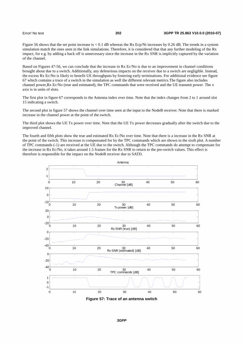
202
3GPP
Error! No text of specified
3GPP TR 25.863 V10.0.0 (2010-07)
Figure 56 shows that the set point increase is < 0.1 dB whereas the Rx Ecp/Nt increases by 0.26 dB. The trends in a system simulation match the ones seen in the link simulations. Therefore, it is considered that that any further modeling of the Rx impact, for e.g. by adding a back off is unnecessary since the increase in the Rx SNR is implicitly captured by the variation of the channel.
Based on Figures 47-56, we can conclude that the increase in Rx Ec/No is due to an improvement in channel conditions brought about due to a switch. Additionally, any deleterious impacts on the receiver due to a switch are negligible. Instead, the excess Rx Ec/No is likely to benefit UE throughputs by fostering early terminations. For additional evidence see figure 67 which contains a trace of a switch in the simulation as well the different relevant metrics.The figure also includes channel power,Rx Ec/No (true and estimated), the TPC commands that were received and the UE transmit power. The x axis is in units of slots.
The first plot in figure 67 corresponds to the Antenna index over time. Note that the index changes from 2 to 1 around slot 15 indicating a switch.
The second plot in figure 57 shows the channel over time seen at the input to the NodeB receiver. Note that there is marked increase in the channel power at the point of the switch.
The third plot shows the UE Tx power over time. Note that the UE Tx power decreases gradually after the switch due to the improved channel.
The fourth and fifth plots show the true and estimated Rx Ec/No over time. Note that there is a increase in the Rx SNR at the point of the switch. This increase is compensated for by the TPC commands which are shown in the sixth plot. A number of TPC commands (-1) are received at the UE due to the switch. Although the TPC commands do attempt to compensate for the increase in Rx Ec/No, it takes around 1.5 frames for the Rx SNR to return to the pre-switch values. This effect is therefore is responsible for the impact on the NodeB receiver due to SATD.
0 10 20 30 40 50 60
1
2
Antenna
0 10 20 30 40 50 60-10
0
10Channel [dB]
0 10 20 30 40 50 60-20
0
20Tx power [dB]
0 10 20 30 40 50 60-40
-20
0Rx SNR (true) [dB]
0 10 20 30 40 50 60-40
-20
0Rx SNR (estimated) [dB]
0 10 20 30 40 50 60
-10
1
TPC commands [dB]
Figure 57: Trace of an antenna switch

203
3GPP
Error! No text of specified
3GPP TR 25.863 V10.0.0 (2010-07)
12.1.3 Beamforming Transmit Diversity
12.1.3.1 DCH Finger and Finger Management
The parameters for the Practical BFTD Algorithm 2 in CELL_DCH as described in section 4.3.2 and are set to 12,48 == ed degree. Two phase shifters are assumed to be used at the UE transmitter side according to the symmetrical
implementation of the algorithm. Other assumptions are shown in table 1.
12.1.3.1.1 Link Simulation Results
The following metrics are used in the performance evaluation of the algorithm:
- Rx Ecp/No Gain = Rx Ecp/No NoTD - Rx Ecp/No OLTD_BF.
- Tx Ecp/No Gain = Tx Ecp/No NoTD - Tx Ecp/No OLTD_BF.
The negative Rx Ecp/No gain at the NodeB is likely to occur due to the phase discontinuities at the Node B receiver, with the consequence that the channel estimation may be impacted. Table 98 shows the link simulation results with Tx antenna correlation 0, where antenna imbalance is the relative power of the secondary antenna with respect to the first antenna.
Table 98: Link Result for an Open Loop Beamforming Algorithm with Tx Correlation 0
Searcher period Rx Ecp/No Gain[dB] Tx Ecp/No Gain[dB]
Imbalance (dB) 3 0 -3 3 0 -3 12 ms PA3 -0.13 -0.01 -0.1 3.5 2 0.6
100 ms PA3 -0.08 -0.03 -0.02 3.5 1.93 0.58 12 ms VA30 -0.3 -0.3 -0.3 1.6 -0.1 -1.4
100 ms VA30 -0.4 -0.44 -0.4 1.53 -0.27 -1.46
Table 99 shows the finger miss detection probability comparison with 0 dB antenna imbalance and 0 Tx antenna correlation. The miss detection probability for a path (of a particular chipx2 peak offset) is defined as the probability when searcher fails to accumulate energy above the searcher threshold.
Table 99: Finger Miss Detection Probability for the Baseline and Beamforming
Searcher period Path 1 Path 2 Path 3 Path 4 Path 5 Path 6
12 ms PA3 (non TD) 2.5 % N/A N/A N/A N/A N/A
100 ms PA3 (non TD) 2.5 % N/A N/A N/A N/A N/A
12 ms PA3 (OLTD BF) 1.7 % N/A N/A N/A N/A N/A
100 ms PA3 (OLTD BF) 1.6 % N/A N/A N/A N/A N/A
12 ms VA30 (non TD) 0.5 % 1.7 % 27.5 % 36.8 % 79.2 % 95.5 %
100 ms VA30 (non TD) 0.5 % 1.6 % 27 % 37.1 % 78.3 % 95.1 %
12 ms VA30 (OLTD BF) 0.2 % 0.9 % 23.5 % 33.7 % 77.4 % 95 %
100 ms VA30 (OLTD BF) 0.14 % 0.56 % 20.5 % 30.8 % 74.8 % 94 %

204
3GPP
Error! No text of specified
3GPP TR 25.863 V10.0.0 (2010-07)
12.1.3.2 Practical Channel Estimation and Time Tracking Loop
12.1.3.2.1 Link Simulation Results
The practical BFTD Algorithm 2 as defined in section 4.3.2 was used in the simulation. The symmetric phase implementation was used in the simulation with phase offset, d = 48 degrees and e = 12 degrees. The antenna imbalance is set to 0 dB and the transmit antenna correlation is 0. The ITU Pedestrian A 3km/hr channel is used in the simulation.
Table 100 shows the Rx Ecp/No and Tx Ecp/No gains for beamforming transmit diversity over the baseline (no TD).
Table 100: Beamforming Transmit Diversity Gains; Practical Algorithm 2 with symmetric phase implementation
Rx Ecp/No [dB] Tx Ecp/No [dB] No TD BFTD Gain [dB] No TD BFTD Gain [dB]
PA3 -18.88 -18.81 -0.07 -18.7 -20.75 2.05
It can be seen from table 101 that there is a small NodeB receiver loss. Table 3 shows the average set point comparisons for the baseline and the practical algorithm. The average set point is computed over the duration of the simulation.
Table 101: Set point comparison between the Baseline and the Practical Beamforming Algorithm 2
Baseline (No TD) Genie SATD Gain [dB] Average Set point [dB] -18.44 -18.18 -0.26
It can be seen from table 101 that there is a difference of ~0.25 dB in the set point between the beamforming and baseline. Since the inner loop power control attempts to maintain the Rx Ec/No at the level of the set point, an increase in the set point would result in an increase in the Rx Ec/No at the receiver. In the following we investigate the source of this difference.
12.1.3.2.2 Observations
Figures 58 and 59 show the CDF of the set point and the estimated Rx Ec/No at the receiver for both beamforming transmit diversity and the baseline.

205
3GPP
Error! No text of specified
3GPP TR 25.863 V10.0.0 (2010-07)
-19.5 -19.3 -19.1 -18.9 -18.7 -18.5 -18.3 -18.1 -17.9 -17.7 -17.5 -17.3 -17.1-170
0.1
0.2
0.3
0.4
0.5
0.6
0.7
0.8
0.9
1
Set Point [dB]
CD
F
Figure 58: CDF of the Set point for practical Beamforming transmit diversity and the baseline (no TD)
-25 -24 -23 -22 -21 -20 -19 -18 -17 -16 -15 -14 -130
0.1
0.2
0.3
0.4
0.5
0.6
0.7
0.8
0.9
1
Rx Ec/No Estimate [dB]
CD
F
Figure 59: CDF of the estimated Rx Ec/No for practical Beamforming transmit diversity and the baseline (no TD)
The set points vary over the duration of the simulation so as to track channel variations (PA3 channel in this case) in order to maintain the residual BLER of 1 % after 4 transmissions. In figure 58, we note that the set point for beamforming is consistently higher than the baseline case for the duration of the simulation. The estimated Rx Ecp/No at the receiver is therefore also slightly higher for beamforming transmit diversity as seen in figure 59.
From the above tables and figures, we see that beamforming transmit diversity requires a higher set point in order to achieve a target residual BLER of 1 % after 4 transmissions. The cause of this increase is further explored by comparing the normalized mean square channel estimation error in both beamforming and the baseline.
The Normalized Mean Square channel estimation Error (NMSE) is defined as:
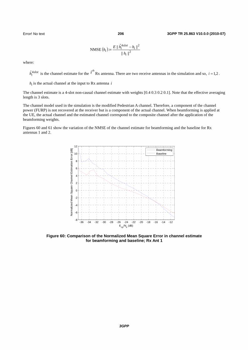
206
3GPP
Error! No text of specified
3GPP TR 25.863 V10.0.0 (2010-07)
( ) 2
24
||||||ˆ||: NMSE
i
islot
ii
hhhEh -=
where:
slotih4ˆ is the channel estimate for the
thi Rx antenna. There are two receive antennas in the simulation and so, 2,1=i .
ih is the actual channel at the input to Rx antenna i
The channel estimate is a 4-slot non-causal channel estimate with weights [0.4 0.3 0.2 0.1]. Note that the effective averaging length is 3 slots.
The channel model used in the simulation is the modified Pedestrian A channel. Therefore, a component of the channel power (FURP) is not recovered at the receiver but is a component of the actual channel. When beamforming is applied at the UE, the actual channel and the estimated channel correspond to the composite channel after the application of the beamforming weights.
Figures 60 and 61 show the variation of the NMSE of the channel estimate for beamforming and the baseline for Rx antennas 1 and 2.
-36 -34 -32 -30 -28 -26 -24 -22 -20 -18 -16 -14 -12-8
-6
-4
-2
0
2
4
6
8
10
12
Ecp/No (dB)
Nor
mal
ized
Mea
n S
quar
e C
hann
el E
stim
atio
n E
rror
[dB
]
BeamformingBaseline
Figure 60: Comparison of the Normalized Mean Square Error in channel estimate for beamforming and baseline; Rx Ant 1

207
3GPP
Error! No text of specified
3GPP TR 25.863 V10.0.0 (2010-07)
-35 -30 -25 -20 -15-8
-6
-4
-2
0
2
4
6
8
10
12
Ecp/No (dB)
Nor
mal
ized
Mea
n S
quar
e C
hann
el E
stim
atio
n E
rror
[dB
]
BaselineBeamforming
Figure 61: Comparison of the Normalized Mean Square Error in channel estimate for beamforming and baseline; Rx Ant 2
It can be seen from figures 60 and 61 that, as expected, the channel estimation quality improves as the Ecp/No at the receiver increases. However, it is also seen that the NMSE in channel estimate is worse than the baseline for the range of Ecp/No values. This is due to the induced fluctuations in the channel on a per slot basis by the beamforming algorithm. Since the channel fluctuates every slot due to the beamforming weights, the application of a multiple-slot non-causal channel estimation algorithm would cause deterioration in the channel estimate. Consequently, a higher Rx Ec/No would be required in order to maintain the same channel estimation quality needed to maintain a residual BLER of 1 %. This would therefore cause the increase in the average set point as seen above in figure 61. However, it is considered that the increase in the Rx Ec/No due to BFTD is not significant enough to cause impact at the NodeB receiver.
12.2 Results for practical Node-B #2 The impact of Switched Antenna Transmit Diversity (SATD) on a practical NodeB receiver is assessed using the practical SATD algorithm described in section 4.3.1. It is assumed that the UE applies a given practical SATD algorithm independently of NodeB (i.e. without informing NodeB) and there are no modifications of practical NodeB receiver algorithms.
The simulation assumptions used for open loop (OL) switched antenna transmit diversity are a subset of assumptions in section 5.1. This simulation was conducted using 2 ms TTI with a TBS of 2020 without outer loop power control. Additionally, the antenna imbalance was assumed to be 0 dB and the Tx and Rx antenna correlations were assumed to be 0. UE DTX was also turned off.
The relative Rx Ec/No gain values for different channel propagation environments are tabulated in table 102. Note that a negative value corresponds to that more power needs to be received at the Node-B.
Table 102: Link-level Simulation Results for the Practical SATD algorithm
Rx Ec/No Gain[dB] Antenna
Correlation (Tx, Rx)
PA3 VA30
VA120
(0, 0) -0.55 -0.6 -0.65

208
3GPP
Error! No text of specified
3GPP TR 25.863 V10.0.0 (2010-07)
13 Summary of RAN WG4 Findings A summary of the RAN WG4 findings on the practical aspects of the ULTD techniques is as follows:
- Performance associated with bursty traffic resulting in state transitions:
· The effect of varying burst sizes and inter-burst time as well the impact of UE state transitions from IDLE to CELL_DCH on ULTD were captured in these simulations for practical ULTD algorithms as described in sections 4.3.1 and 4.3.2.
- In terms of average burst rate gain:
· SATD offers an average burst rate gain ranging from 2 % to 8 % in a PA3 channel setting. For VA30 channel, the gain in average user burst rate ranges from 1 % up to 5 %.
· BFTD offers up to 7 % gain in average user burst rate in a PA3 channel setting. For VA30 channel, no substantial improvement or degradation in terms of average user burst rate is observed.
- In terms of 10th percentile user burst rate:
· SATD offers up to 31 % improvement for PA3 channel and up to 16 % improvement for VA30 channel, thereby improving cell-edge user experience.
· BFTD offers up to 40 % improvement for PA3 channel and up to 14 % improvement for VA30 channel, thereby improving cell-edge user experience.
- Demodulation losses due to studied uplink transmit diversity techniques:
· It was acknowledged that these techniques can impact NodeB receiver performance. For the ULTD algorithms simulated, assuming practical NodeB receivers, the impact to NodeB receiver performance was difficult to conclude on, due to the fact that some results were attributed to the particular ULTD algorithms and the NodeB receiver used in simulations. For the practical SATD algorithm studied in the report, some results with a realistic NodeB implementation suggested that up to 0.65 dB (or ~16 %) more power would need to be received at the NodeB to obtain the same quality. For a sub-optimal BFTD algorithm studied in this report, using the same practical NodeB receiver, a significant impact (up to 2.6 dB or 81 %) on received power was observed. On the other hand, for other ULTD algorithms that were evaluated assuming a different NodeB receiver, it was observed that the impact to the DPCCH set-point was observed to be < 0.1 dB for SATD and ~0.25 dB for BFTD for the commonly agreed simulation assumptions. Hence the impact to NodeB receiver performance can be concluded to depend on the ULTD algorithm and the practical NodeB receiver. However, no consensus regarding the amount of typical demodulation losses for SATD or BFTD was reached since the details of one of the NodeB receivers could not be disclosed.
· It was also shown that the BFTD algorithm is very sensitive to the mismatch in TPC delay assumed by the UE compared to the actual TPC delay introduced by the NodeB. Although, potential algorithms can be devised at the UE to try estimate the TPC delay, the feasibility of testing whether a UE was estimating the correct TPC delay or not is not clear. In particular, due to the lack of a reference NodeB power control implementation in the test setup, it was not clear how best to emulate the TPC bit generation that could happen in a practical NodeB receiver.
- For both transmit diversity schemes (i.e. BFTD and SATD) a negative Rx Ec/N0 was observed in different propagation conditions, i.e. the Rx Ec/N0 was increased in the presence of open loop transmit diversity.
- Effects from mixes of different uplink Tx diversity algorithms and/or legacy UEs:
· Some results have shown that with different penetration levels, ranging from 25 % to 75 %, there are minor throughput and Tx-power gains for TX diversity users but at the same time some configurations can have impact on the performance experienced by non-TX diversity UEs. The degradation to non-TX diversity UEs was especially clear at larger ISD, when the non-TXD users are power limited. The simulations were performed

209
3GPP
Error! No text of specified
3GPP TR 25.863 V10.0.0 (2010-07)
assuming that all the Tx Diversity UEs were applying the same algorithms. The impact on the system performance when a mix of different ULTD algorithms were used by the UEs in the system, was not studied.
· However, in another set of results, where UL was RoT limited rather than power limited (lower ISD), it was observed that when partial introduction of Tx Diversity enabled UEs is done, the gains were similar to the 100 % penetration case. At the same time, small gains were observed for the legacy UEs.
· One possible explanation to the difference in results is that different schedulers have been assumed.
- System impact of ULTD in high velocity propagation conditions:
· A study was performed for both SATD and BFTD for the VA120 km/hr propagation channel. A substantial loss was observed in terms of mean user throughput and mean cell throughput when the long-term antenna imbalance is -4 dB. Furthermore, the reduction in UE transmit power was very small for the cases considered. It was proposed by two companies that in order to prevent the negative impact on the system performance in certain radio environments the possibility should exist for the network to control the ULTD operation. It was also pointed out that such control could exist in the ULTD algorithm itself that relies on a coarse estimate of the UE speed. It was on the other hand argued by another company that autonomous control of the ULTD diversity is less favourable to allow, because of the risk for system degradation due to the network not having control of the UE behaviour and due to large inaccuracies involved in speed estimation especially when DRX/DTX is used.
· In order to prevent the negative impact on the system performance in certain radio environments we clearly see the benefit of having the possibility for the network to control the SATD operation.
- Performance of suboptimal ULTD algorithms:
· In a study for the PA3 km/hr, the performance of a suboptimal SATD algorithm was evaluated. This was modelled by letting the UE take a random decision for a certain part of the radio frames. It was observed that the performance degradation was dependent on the level of randomized behaviour of the UE algorithm and performance degrades also for algorithms that are only slightly imperfect. This indicates that the system performance may be sensitive to what type of ULTD algorithm that the UE is utilizing.
- Interaction with DC-HSUPA:
· The co-existence of open loop transmit diversity with DC-HSUPA has not been studied.
- UE battery and heat savings
· UE battery and heat savings analysis was performed using two different methodologies that assumed practical PA efficiency curves.
- One methodology was based on using two UE transmit power profiles 1) due to the CDG35 user transmit power profile; and 2) due to HSUPA traffic from a UE located at one fixed stationary position at cell-edge in a live network. Each of these UE transmit power profiles were then used along with the PA efficiency curve to evaluate the potential gains in UE battery and heat consumption for a range of transmit power reductions of the same order as observed in the link and system study for both SATD and BFTD. Using this methodology, for a 2 dB reduction in transmit power, BFTD offered up to ~18% savings in PA power consumption while for a 1.5 dB reduction in UE average transmit power, SATD offered up to ~8 % savings in PA power consumption. In practice the size of the gain will be highly dependent on the average reduction in Tx power and it should be noted that for the VA30 channel the observed gains were in general closer to 1 dB for BFTD and 0.5 dB for SATD. It should also be noted that the study focused on a specific PA design and that the end results might differ when other PA designs are considered.
- Another methodology was based on evaluating the battery life gains of SATD in a system simulation. The simulation did consider the power consumption only in the PA. The simulation did not assume any additional demodulation losses (in case such demodulation losses occur this could result in a smaller gain in PA power consumption). It assumed a long-term antenna imbalance of 0 dB for the second transmit antenna, an ideal path searcher, and accounted for an insertion loss introduced by the RF switch. Based on an insertion loss of 0.8 dB, the analysis was shown to demonstrate an increase in average power consumption by the PA with up to 17.5 % for the VA30 channel. For a more optimistic insertion loss of 0.3 dB, the increase was in the order

210
3GPP
Error! No text of specified
3GPP TR 25.863 V10.0.0 (2010-07)
of 4 %. For the PA3 channel model the study showed results ranging from a reduction in PA power consumption of 2.5 % to an increase in PA power consumption of 8 %, as the insertion loss increased from 0.3 dB to 0.8 dB. It should be noted that the PA power will dominate in the UE power consumption when the UE transmits at close to maximum transmit power.
- PRACH coverage impact due to BFTD:
· One of the candidate UE architectures was discussed which allowed the UE to use a full power PA in Idle or CELL_FACH state thereby ensuring that the PRACH coverage remained unaltered. The same UE when transmitting in CELL_DCH was shown to operate in two half-power PA mode, when BFTD is enabled using the technique of dynamic voltage scaling. Hence it was concluded that using such a UE architecture, enabling BFTD in the UE in CELL_DCH could have no impact on UL PRACH coverage. However, to guarantee that the UL PRACH coverage is not degraded it would be necessary to ensure that BFTD UEs only transmit from one antenna (thus at least one full power PA would always be needed).
- Impacts on UE implementation:
· Impacts to UE implementation were identified. Besides the introduction of control logic to support the ULTD algorithms, it was identified that additional duplexer, and an additional transmit antenna would be required at the UE for both SATD and BFTD. In addition for SATD, a RF switch would be required to support the antenna switching operation while for BFTD, a second power amplifier (PA) would be required. Some of these components would need to be specific for the frequency band on which UL TXD is supported. For SATD, it was also noted that unless the specification allows for a maximum power reduction to mitigate the effect of additional insertion loss due to the switch, the PA size would need to be increased.
- Impact on existing UE core requirements:
· The impact analysis on UE Tx core requirements due to SATD was discussed. In particular, it was argued by one company that since the UE architecture for SATD uses the same transmit chain as for the case when SATD is disabled, there is no impact to all but 1 of the Tx core requirements. In particular, due to the presence of an RF switch, if the PA design used in existing architectures is not modified, it is expected that some relaxation may be beneficial with regard to the UE maximum output power requirement (6.2.1 in 25.101). In situations where SATD is not enabled this may reduce uplink coverage for these UEs (the magnitude will be dependent on the size of the relaxation). Furthermore due to the existence of a second duplexer and a second antenna, it was considered necessary that the UE be manually configured to transmit on the second antenna and test for 1) UE maximum output power, 2) Spurious Emissions (6.6.3) and Error Vector Magnitude (6.8.2).
· With regard to UE Rx core requirements, it was suggested that there may be a need to test the receiver performance against existing requirements by manually configuring the UE to transmit on each antenna separately so as to capture the impact of the Tx/Rx isolation due to each of the duplexers.
- Introduction of new core Tx requirements:
· It was discussed whether it would be possible to devise sufficient test coverage for UEs employing open loop transmit diversity, since there are no specifications detailing the UE behavior. It was argued by some companies that the requirements should focus on a few selected architectures, while other companies argued that no specific architecture could be assumed when devising the test because of the lack of specification on UE behavior. It was discussed whether the tests could employ an initialization phase that would identify specific UE architectures and adapt the testing accordingly, no consensus was however reached on whether this would be feasible.
· For SATD, the following new core Tx requirements were proposed by the proponents of the architecture specific test approach :
- A limit on the antenna switching rate to ensure minimal impact to NodeB receiver performance. Further work would be needed to determine suitable TPC bit patterns to ensure that the UE does not exceed this limit.
- In addition to a switching rate limit, the need for additional TX core requirements to ensure minimal impact to node B receiver was discussed but not concluded.

211
3GPP
Error! No text of specified
3GPP TR 25.863 V10.0.0 (2010-07)
- It was also pointed out by a few companies that further study may be needed during any possible work item to evaluate if there is a need to specify a requirement on the power emitted by the unused antenna port thereby limiting the amount of leakage introduced by the switch from the active transmit path.
· The need for additional TX requirements to ensure the gains of TX diversity were realized was discussed, but the feasibility of such requirements was not concluded.
14 Conclusion A link and system study was carried out by RAN WG1 to investigate UL Tx diversity techniques for HSPA under the constraint that no new standardised dynamic feedback signalling would be required between network and UE. In particular, both forms of transmit diversity, 1) switched antenna Tx diversity (simultaneous transmission from 1 transmit antenna) and 2) beamforming (simultaneous transmission from 2 Tx antennas) were thoroughly investigated. In general potential gains (or losses) from ULTD in terms of throughput and power saving varied between scenarios and companies. One potential explanation for the latter was that different companies assume different Node-B schedulers. For slow fading propagation conditions some gains for the average and 10th percentile user throughputs for the TX-diversity users were noticed. In other scenarios (fast fading, negative long term antenna imbalance), smaller gains or some losses were also observed. A detailed conclusion on the system evaluation of these techniques and the set of assumptions on which the results rely can be found in section 7.3.
RAN WG4 further discussed the practical aspects of these techniques. In general, there were agreements on a few topics including 1) impact on UE implementation, 2) partial agreement on impact on existing core requirements such as the need for relaxing the UE maximum output power requirement, 3) bursty traffic system performance under the assumption that there would be no additional Node-B demodulation losses,4) System performance degradation due to incorrect TPC delay It was considered that the UE modifications to support ULTD operation were feasible. It was also argued by one company that the difficulty to devise appropriate test-cases might induce a risk for system performance degradation... It was also acknowledged that some relaxation would be required with regard to the UE maximum output power requirement for SATD operation in order to overcome the additional transmit chain insertion loss due to the added circuitry associated with the feature.. Finally, it was agreed that incorrect estimate of delays corresponding to TPC commands at the UE causes negative impacts to open loop beamforming.
However, it was difficult to arrive at a consensus on the following topics:
- NodeB Demodulation losses associated with various possible algorithms.
- Effects from mixes of different uplink Tx diversity algorithms and/or legacy UEs.
- Feasibility of testing of new core Tx requirements.
- Feasibility of testing TPC delay correctness.
- UE battery power and heat savings.
More details on the RAN WG4 findings can be found in section 13.
Based on the study performed here, it is considered that the UL Transmit Diversity techniques for HSPA can help improve the uplink coverage for TX-diversity users in some scenarios, while marginally improving system performance with large penetration of TX-diversity capable UE's.. It should be noted that there were some potential system performance concerns raised under some conditions (eg. sub-optimal transmit diversity algorithms, high velocity propagation conditions along with zero antenna correlation and negative long term antenna imbalance) due to implications to non-TX-diversity users performance, and due to impact on the legacy Node B performance. For this purpose, it was recommended that higher layer signaling to enable/disable the uplink transmit diversity transmission should be considered as a possible method to mitigate some of these concerns, although it has not been evaluated whether such signaling can be effectively used in a dynamic manner. It should also be noted that the co-existence of open loop uplink transmit diversity with DC-HSUPA has not been studied.

212
3GPP
Error! No text of specified
3GPP TR 25.863 V10.0.0 (2010-07)
Annex A (informative): Change history
Change history Date TSG # TSG Doc. CR Rev Subject/Comment Old New 2010-01 R1#59bi Initial Draft. 0.1.0
2010-02 R4#54 RAN4 related 25.863 TR skeleton for UL transmit diversity 0.2.0 2010-05 R4#55 Updated 25.863 TR skeleton for UL transmit diversity 0.3.0 2010-05 R4#55 Updated 25.863TR for UL Transmit Diversity 0.3.0 2010-06 RP#48 RP-100646 Presental to TSG RAN for approval 0.3.0 2.0.0 2010-06 RP#48 RP-100646 Approved by TSG RAN 2.0.0 10.0.0