Embed Size (px)
Citation preview
RISA3D
Rapid Interactive Structural Analysis – 3 Dimensional
Verification Problems
26632 Towne Centre Drive, Suite 210 Foothill Ranch, California 92610 (949) 951‐5815 (949) 951‐5848 (FAX) www.risatech.com
Copyright 2012 by RISA Technologies, LLC. All rights reserved.
No portion of the contents of this publication may be reproduced or transmitted in any means without the express written permission of RISA Technologies, LLC.
We have done our best to insure that the material found in this publication is both useful and accurate. However, please be aware that errors may exist in this publication, and that RISA
Technologies, LLC makes no guarantees concerning accuracy of the information found here or in the use to which it may be put.

i
Table of Contents
Verification Overview ............................................................................................................................................................ 1
Verification Problem 1: Truss Model‐ Axial Loads .................................................................................................... 2
Verification Problem 2: Cantilever Model Deflections ............................................................................................. 4
Verification Problem 3: Member Force Comparison ................................................................................................ 6
Verification Problem 4: Thermal Loads ......................................................................................................................... 8
Verification Problem 5: Hot Rolled Steel Frame Design ........................................................................................ 10
Verification Problem 6: Spiral Staircase‐Force Comparison ............................................................................... 40
Verification Problem 7: Beam Frequency Model ...................................................................................................... 42
Verification Problem 8: Plate Element Bending ....................................................................................................... 44
Verification Problem 9: Dynamic and Response Spectra Analysis ................................................................... 47
Verification Problem 10: Wood Frame Design .......................................................................................................... 50
Verification Problem 11: Tapered Hot Rolled WF Comparison ......................................................................... 62
Verification Problem 12: P‐Delta Displacements ..................................................................................................... 66
Verification Problem 13: Projected Loads Comparison ........................................................................................ 72
Verification Problem 14: Solid Element Deflection ................................................................................................. 74

1
Verification Overview Verification Methods We at RISA Technologies maintain a library of dozens of test problems used to validate the computational aspects of RISA programs. In this verification package we present a representative sample of these test problems for your review.
These test problems should not necessarily be used as design examples; in some cases the input and assumptions we use in the test problems may not match what a design engineer would do in a “real world” application. The input for these test problems was formulated to test RISA‐3D’s performance, not necessarily to show how certain structures should be modeled. The RISA‐3D solutions for each of these problems are compared to either hand calculations or solutions from other well established programs. By “well established” we mean programs that have been in general use for many years, such as the Berkeley SAPIV program. The original SAPIV program is still the basis for several commercial programs currently on the market (but not RISA‐3D).
The reasoning is if two or more independently developed programs that use theoretically sound solution methods arrive at the same results for the same problem, those results are correct. The likelihood that both programs will give the same wrong answers is considered extremely remote.
If discrepancies occur between the RISA‐3D and the SAPIV results during testing, we don’t automatically assume SAPIV is correct. Additional testing and hand calculations are used to verify which solution (if either) is correct. There are instances where SAPIV results have been proven to be incorrect.
The data for each of these verification problems is provided. The files are Verification Problem 1.r3d for problem 1, Verification Problem 2.r3d for problem 2, etc. When you install RISA‐3D these data files are copied into the C:\RISA\Examples directory. If you want to run any of these problems yourself, just read in the appropriate data file and have at it.
Verification Version This document contains problems that have been verified in RISA‐3D version 10.0.1.
2
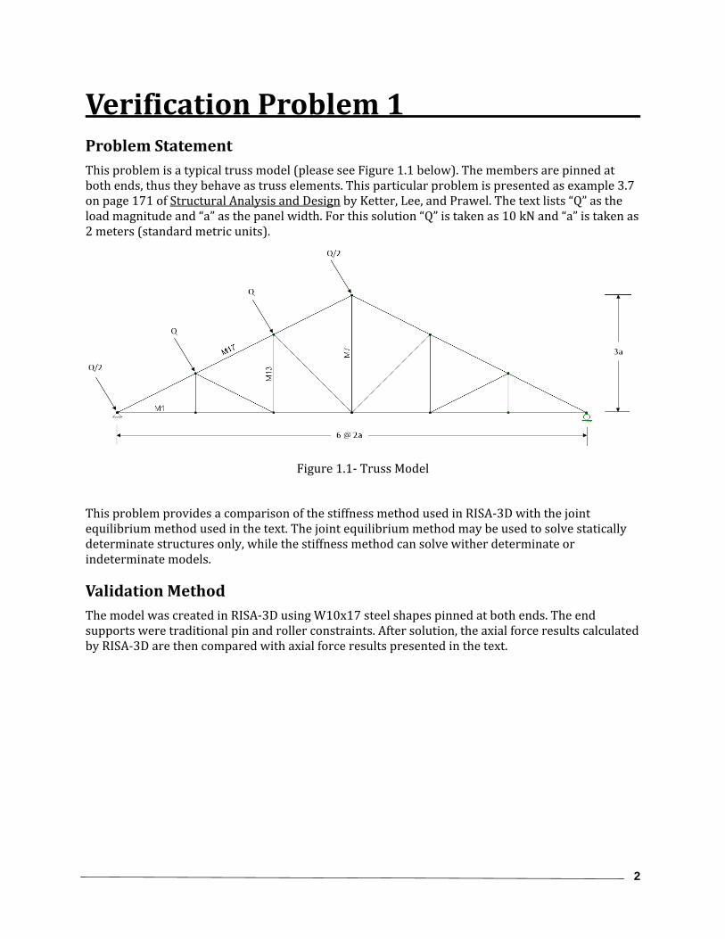
Verification Problem 1 Problem Statement This problem is a typical truss model (please see Figure 1.1 below). The members are pinned at both ends, thus they behave as truss elements. This particular problem is presented as example 3.7 on page 171 of Structural Analysis and Design by Ketter, Lee, and Prawel. The text lists “Q” as the load magnitude and “a” as the panel width. For this solution “Q” is taken as 10 kN and “a” is taken as 2 meters (standard metric units).
Figure 1.1‐ Truss Model
This problem provides a comparison of the stiffness method used in RISA‐3D with the joint equilibrium method used in the text. The joint equilibrium method may be used to solve statically determinate structures only, while the stiffness method can solve wither determinate or indeterminate models.
Validation Method The model was created in RISA‐3D using W10x17 steel shapes pinned at both ends. The end supports were traditional pin and roller constraints. After solution, the axial force results calculated by RISA‐3D are then compared with axial force results presented in the text.
3
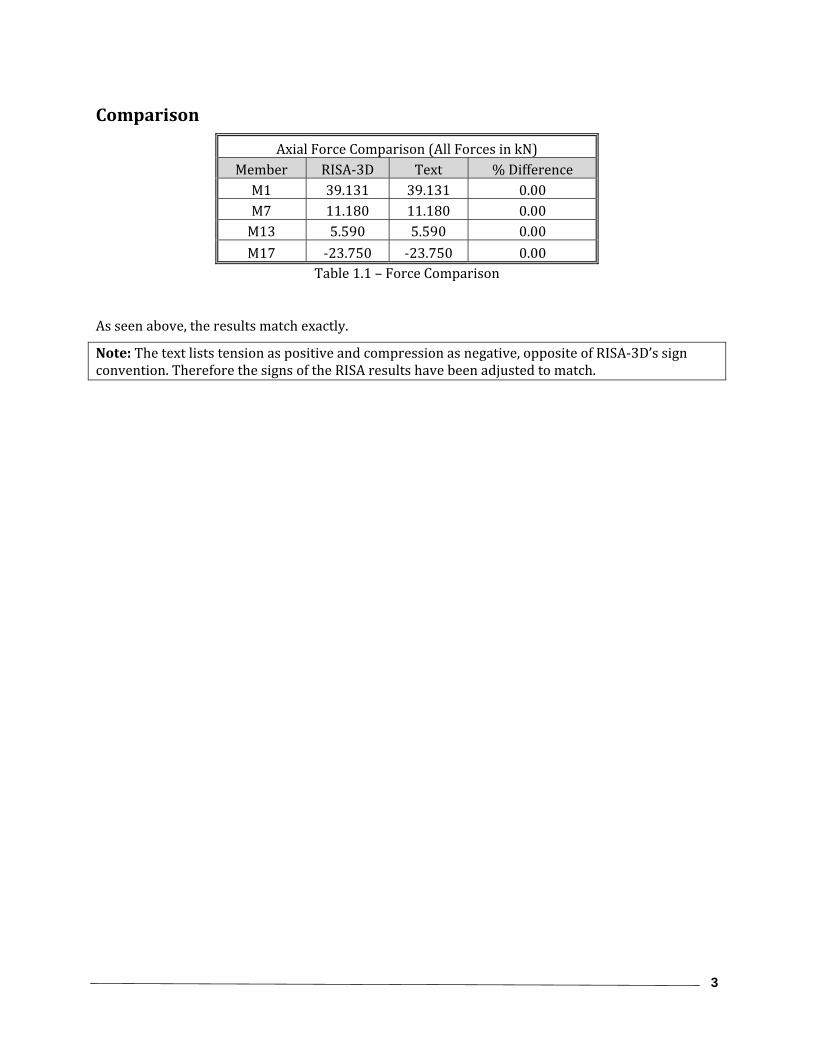
Comparison
Axial Force Comparison (All Forces in kN) Member RISA‐3D Text % Difference M1 39.131 39.131 0.00 M7 11.180 11.180 0.00 M13 5.590 5.590 0.00 M17 ‐23.750 ‐23.750 0.00
Table 1.1 – Force Comparison
As seen above, the results match exactly.
Note: The text lists tension as positive and compression as negative, opposite of RISA‐3D’s sign convention. Therefore the signs of the RISA results have been adjusted to match.
4
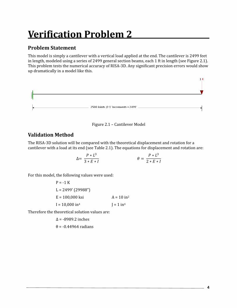
Verification Problem 2 Problem Statement This model is simply a cantilever with a vertical load applied at the end. The cantilever is 2499 feet in length, modeled using a series of 2499 general section beams, each 1 ft in length (see Figure 2.1). This problem tests the numerical accuracy of RISA‐3D. Any significant precision errors would show up dramatically in a model like this.
Figure 2.1 – Cantilever Model
Validation Method The RISA‐3D solution will be compared with the theoretical displacement and rotation for a cantilever with a load at its end (see Table 2.1). The equations for displacement and rotation are:
∆ 3
2
For this model, the following values were used:
P = ‐1 K
L = 2499’ (29988”)
E = 100,000 ksi A = 10 in2
I = 10,000 in4 J = 1 in4
Therefore the theoretical solution values are:
Δ = ‐8989.2 inches
θ = ‐0.44964 radians

5
Comparison
Cantilever Solution Comparison (Standard Skyline Solver) Value RISA‐3D Theoretical % Difference
Displacement (in) ‐8989.29 ‐8989.2 0.0010 Rotation (rad) ‐0.4496 ‐0.44964 ‐0.0089
Cantilever Solution Comparison (Sparse Accelerated Solver) Value RISA‐3D Theoretical % Difference
Displacement (in) ‐8989.28 ‐8989.2 0.0009 Rotation (rad) ‐0.4496 ‐0.44964 ‐0.0089
Table 2.1 – Results Comparison
As seen above, the results match exactly or have negligible difference.

6
Verification Problem 3 Problem Statement This model is a small 3D frame with oblique members (see Figure 3.1). The purpose of this model is to test RISA‐3D’s handling of member loads. The members in this model are loaded with full distributed loads, partial length distributed loads, point loads, joint loads, and moments in various load combinations.
In some cases, the loads are used to test RISA‐3D against itself. For example, the self weight capability will also be tested by calculating a set of distributed loads equivalent to the member’s self weight. The solution for these applied loads is compared to the RISA‐3D automatic self weight calculation.
Figure 3.1 – Frame Model
Validation Method The RISA‐3D results are compared with the solution of this model using the Berkeley SAPIV program (see Table 3.1). SAPIV has been used widely in various forms for well over 20 years. Many commercial programs currently on the market can be traced back to the original SAPIV program.

7
Comparison
Member Force Comparison: RISA‐3D vs. SAPIV Member Load Combination Force RISA‐3D SAPIV % Difference M1 7 Axial (k) 8.8776 * 0.057 M1 7 Axial (k) 8.8827 * 0.057 M9 3 Axial (k) ‐17.3595 ‐17.35 0.055 M9 5 Mz (k‐ft) ‐10.1512 ‐10.15 0.012 M9 6 My (k‐ft) 7.5346 7.53 0.061 M10 2 Mz (k‐ft) 18.6057 18.61 0.023 M10 6 Mz (k‐ft) ‐31.7113 ‐31.7 0.036 M11 1 Mz (k‐ft) ‐10.6905 ‐10.69 0.005 M11 5 My (k‐ft) 2.4596 2.45 0.390 M11 6 Z‐ Shear (k) ‐7.7985 ‐7.8 0.019 M12 4 My (k‐ft) 4.4767 4.48 0.074 M12 5 Y‐Shear (k) 3.8802 3.88 0.005
*These results are those in which RISA‐3D tested against itself. Load Case 7 is the self weight defined as applied loads. Load Case 8 is the automatic self weight calculation, so compare Load Case 7 results to those of Load Case 8.
Table 3.1 – Force Comparison
As can be seen above, the results match very closely. Any slight variations in the results can be attributed to round off differences.

8
Verification Problem 4 Problem Statement This model is used to test the thermal force calculations in RISA‐3D. The model is a five member cantilever with a spring in the local x direction at the free end (see Fig. 4.1). As the model is loaded thermally the spring resist some, but not all, of the thermal expansion.
Thermal loads cause structural behavior somewhat different from other loads. For gravity loads, displacements induce stress; but for thermal loading, displacements cause stress to be relieved. For example, a free end cantilever that undergoes a thermal loading would expand without resistance and thus no stress. Conversely, a fixed‐fixed member that undergoes the same thermal loading would see a stress increase with no displacements.
This model uses a spring to provide partial resistance to the thermal load. This is realistic in that members generally would have only partial resistance to thermal effects.
Figure 4.1 – Thermal Model
Validation Method The model is validated by the use of hand calculations (see Table 4.1). The theoretically exact solution may be calculated for comparison with the RISA‐3D result. Following are those calculations:
Property Values:
Area (A) = 50 cm2
Young’s Modulus (E) = 70,000 MPa
Thermal Load (ΔT) = 300°
Coefficient of Thermal Expansion (α) = 0.000012 cm/cm°C
Spring Stiffness (K) = 500 kN/cm
Length (L) = 10 meters
The unrestrained thermal expansion (∆Free) is:
∆ ∆
The general equation for the displacement of a member due to an axial load (∆Axial) is:
∆
9
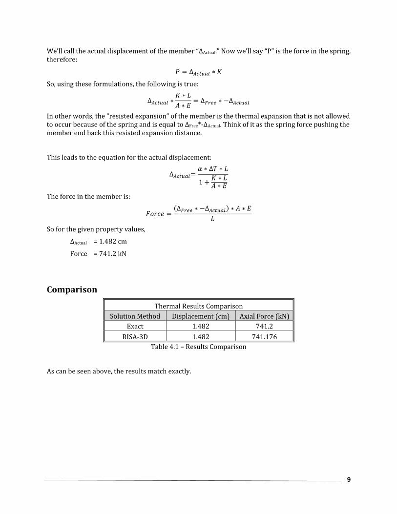
We’ll call the actual displacement of the member “∆Actual.” Now we’ll say “P” is the force in the spring, therefore:
∆
So, using these formulations, the following is true:
∆ ∆ ∆
In other words, the “resisted expansion” of the member is the thermal expansion that is not allowed to occur because of the spring and is equal to ∆Free*‐∆Actual. Think of it as the spring force pushing the member end back this resisted expansion distance.
This leads to the equation for the actual displacement:
∆∆
1
The force in the member is: ∆ ∆
So for the given property values,
∆Actual = 1.482 cm
Force = 741.2 kN
Comparison
Thermal Results Comparison Solution Method Displacement (cm) Axial Force (kN)
Exact 1.482 741.2 RISA‐3D 1.482 741.176
Table 4.1 – Results Comparison
As can be seen above, the results match exactly.
10
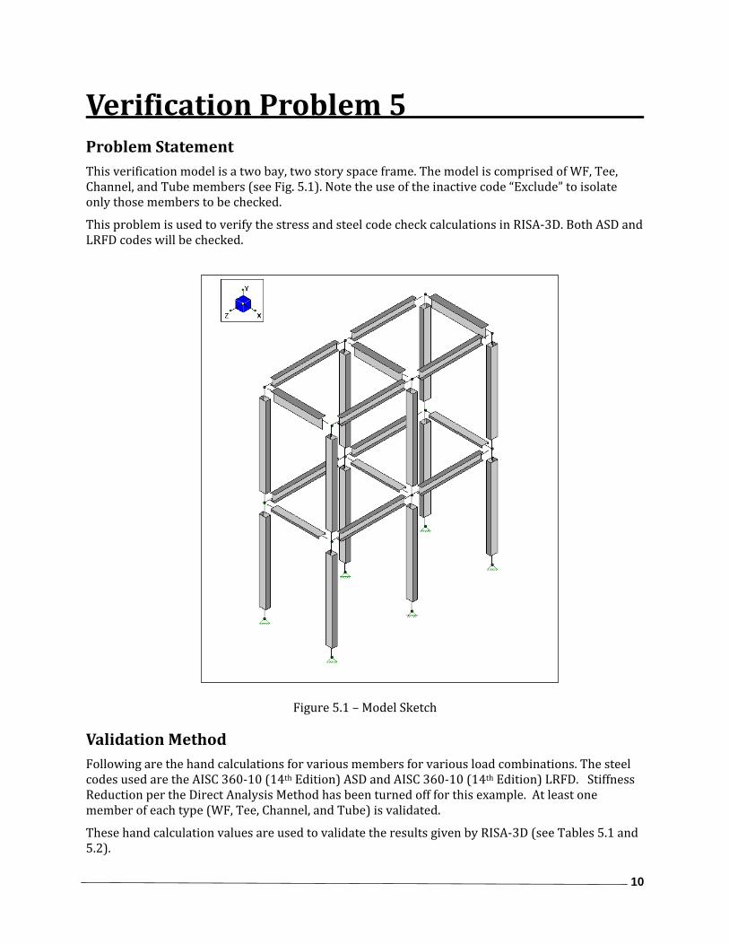
Verification Problem 5 Problem Statement This verification model is a two bay, two story space frame. The model is comprised of WF, Tee, Channel, and Tube members (see Fig. 5.1). Note the use of the inactive code “Exclude” to isolate only those members to be checked.
This problem is used to verify the stress and steel code check calculations in RISA‐3D. Both ASD and LRFD codes will be checked.
Figure 5.1 – Model Sketch
Validation Method Following are the hand calculations for various members for various load combinations. The steel codes used are the AISC 360‐10 (14th Edition) ASD and AISC 360‐10 (14th Edition) LRFD. Stiffness Reduction per the Direct Analysis Method has been turned off for this example. At least one member of each type (WF, Tee, Channel, and Tube) is validated.
These hand calculation values are used to validate the results given by RISA‐3D (see Tables 5.1 and 5.2).
11
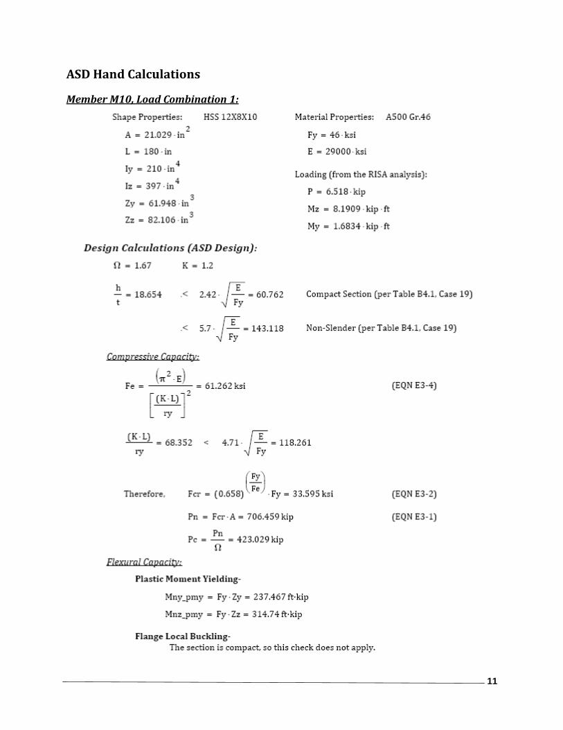
ASD Hand Calculations
Member M10, Load Combination 1:
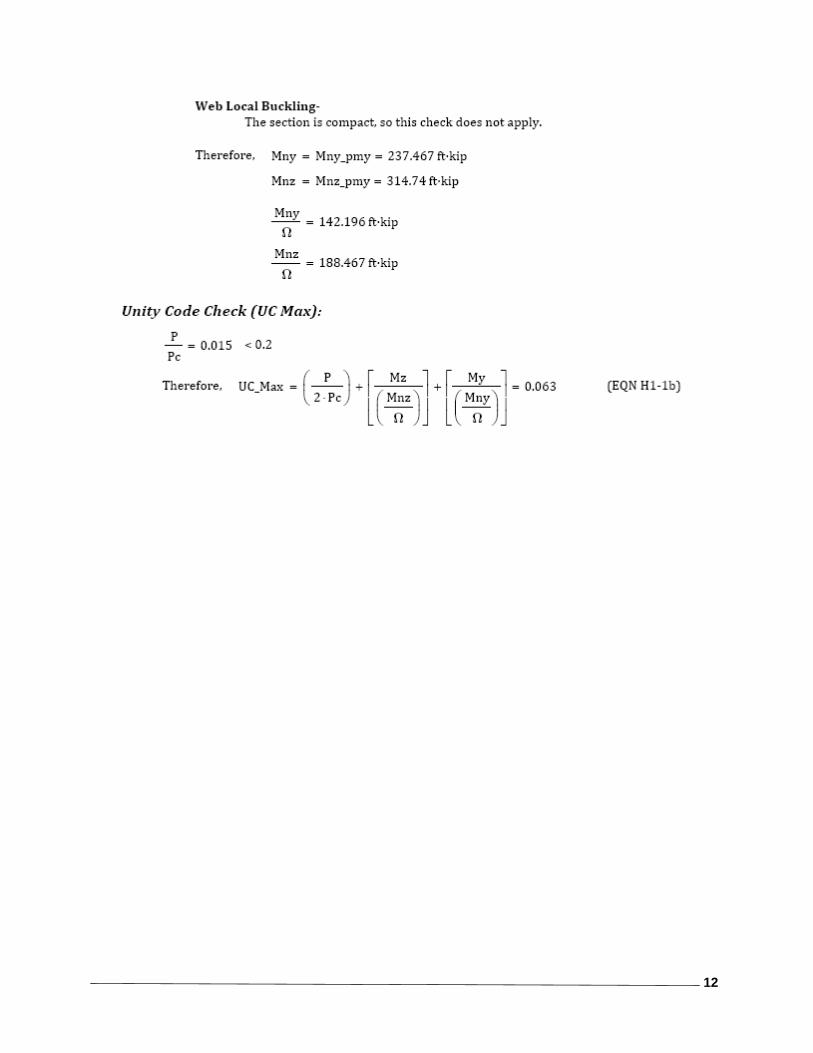
12
13
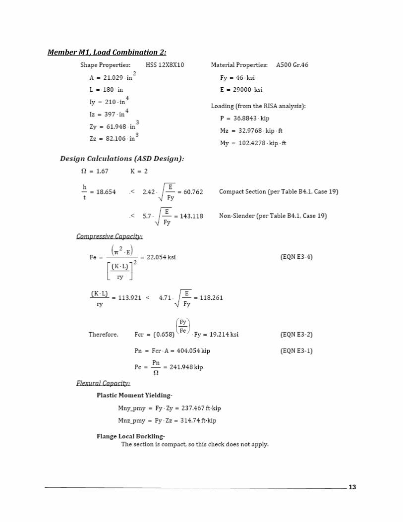
Member M1, Load Combination 2:

14

15
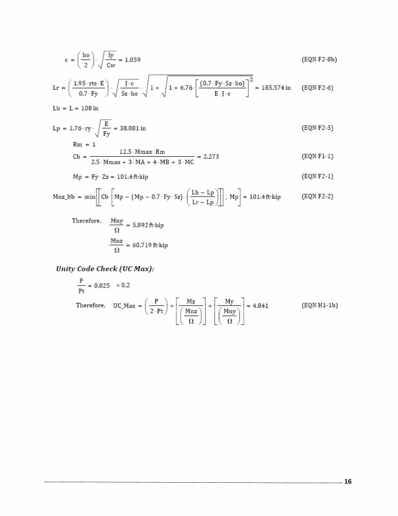
Member M14, Load Combination 3:
16

17
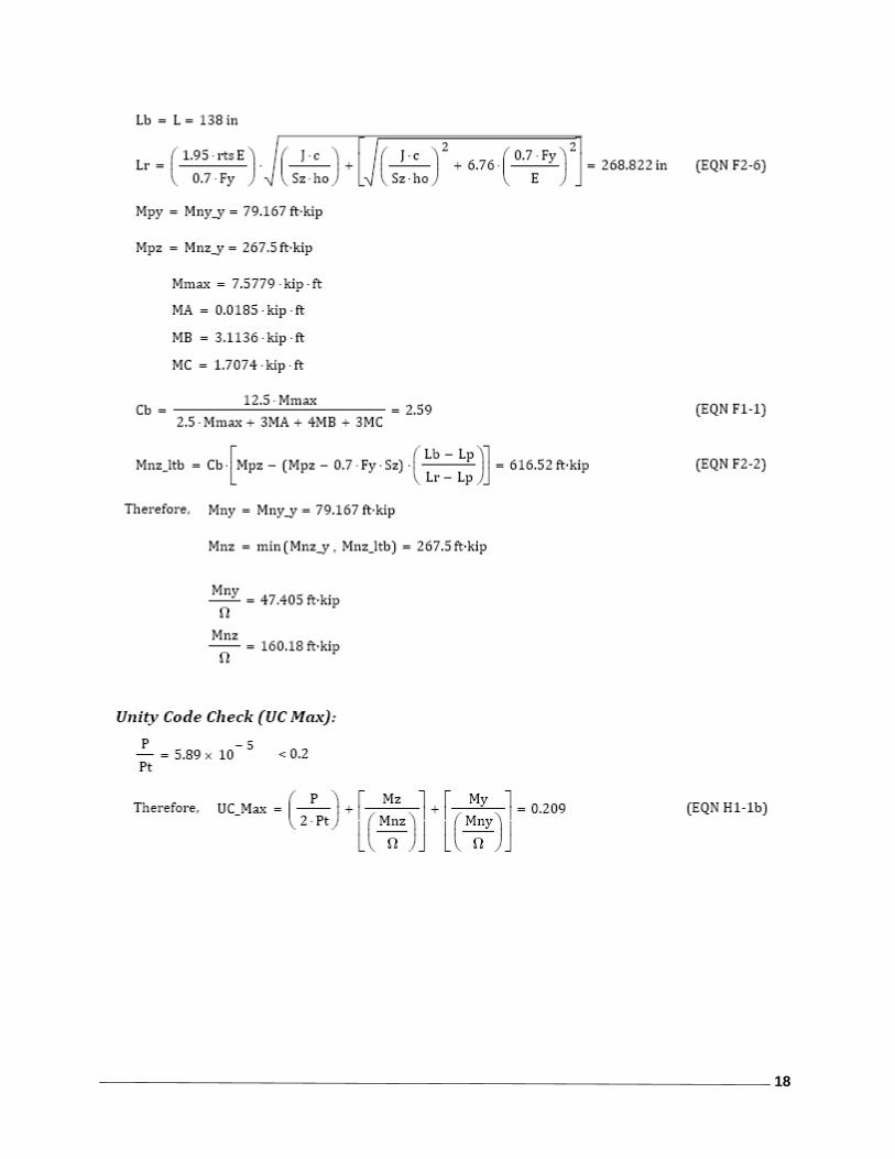
Member M25, Load Combination 2:
18
19
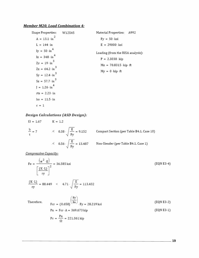
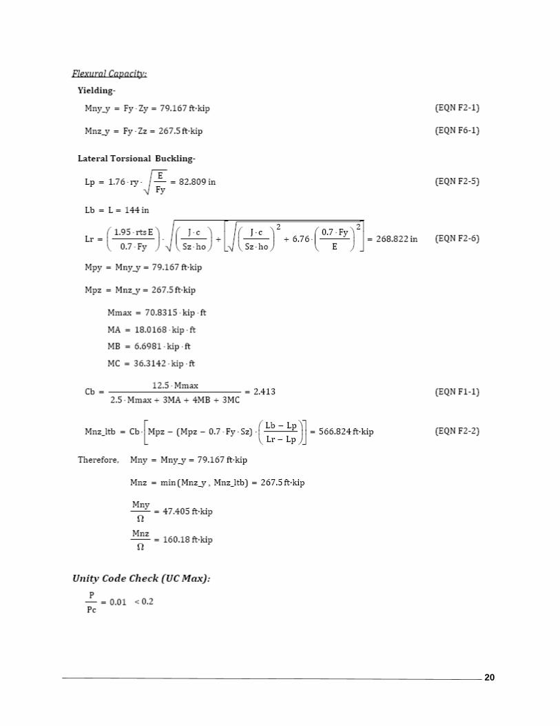
Member M20, Load Combination 4:
20

21
22
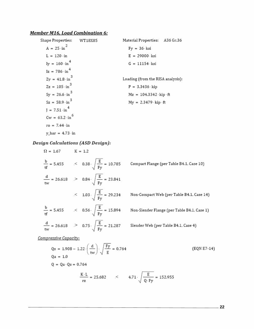
Member M16, Load Combination 6:

23
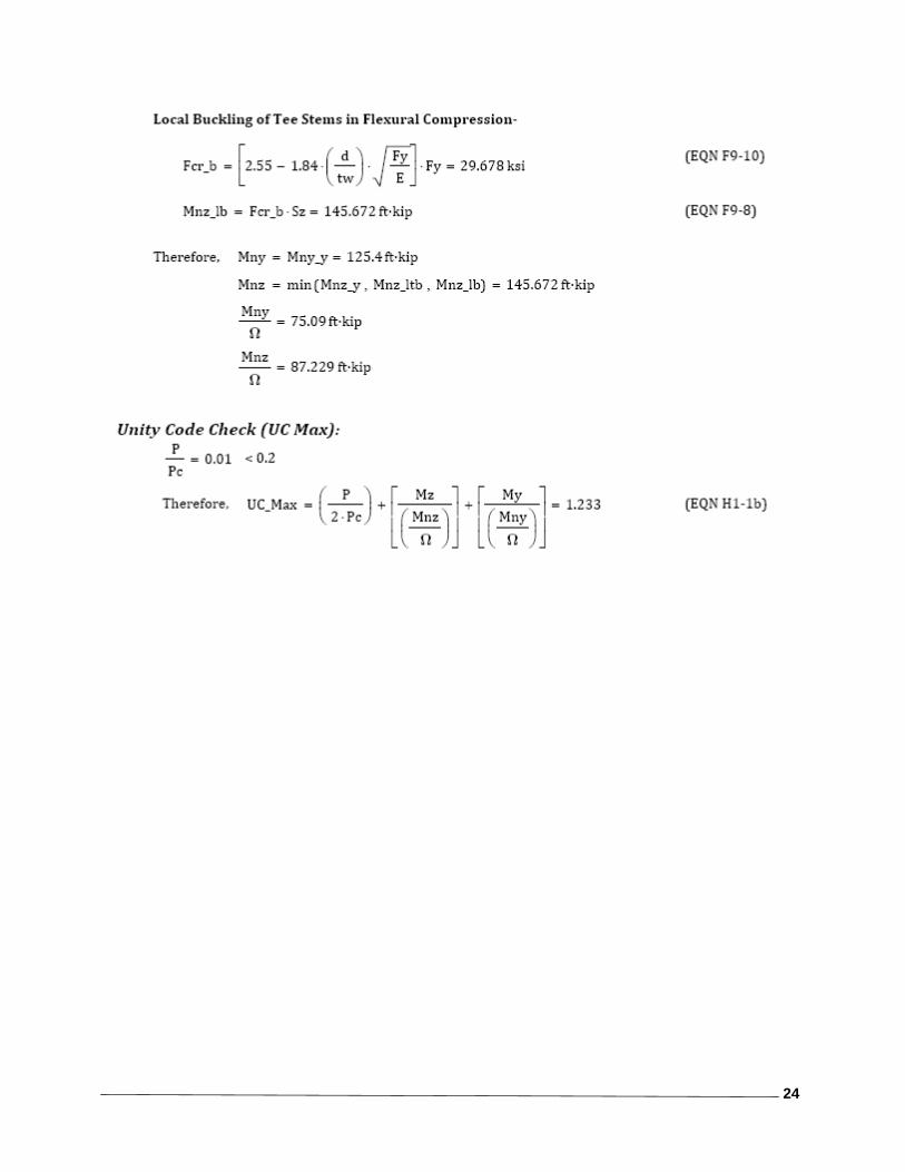
24

25
ASD Results Comparison
ASD Unity Check Comparisons Member Load Combination RISA‐3D Hand Calculations % Difference M10 1 0.063 0.063 0.000 M1 2 0.972 0.972 0.000 M14 3 4.84 4.841 0.021 M25 2 0.212 0.209 1.435 M20 4 0.447 0.447 0.000 M16 6 1.235 1.233 0.162
Table 5.1 – ASD Comparisons
As can be seen in the chart above, the results match almost exactly. Any slight differences can be attributed to round off error or torsional effects.

26
LRFD Hand Calculations
Member M10, Load Combination 10:
27
28
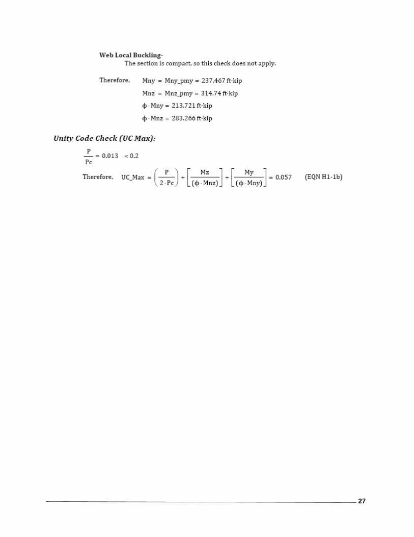
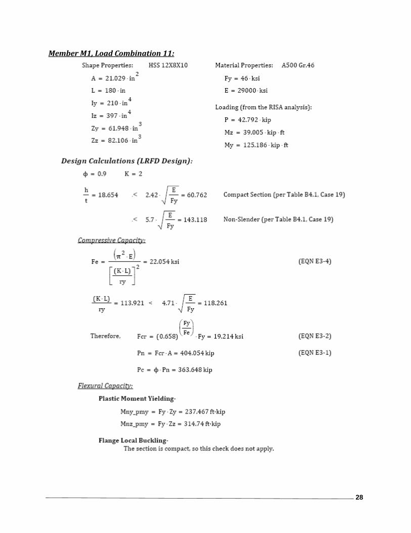
Member M1, Load Combination 11:

29
30
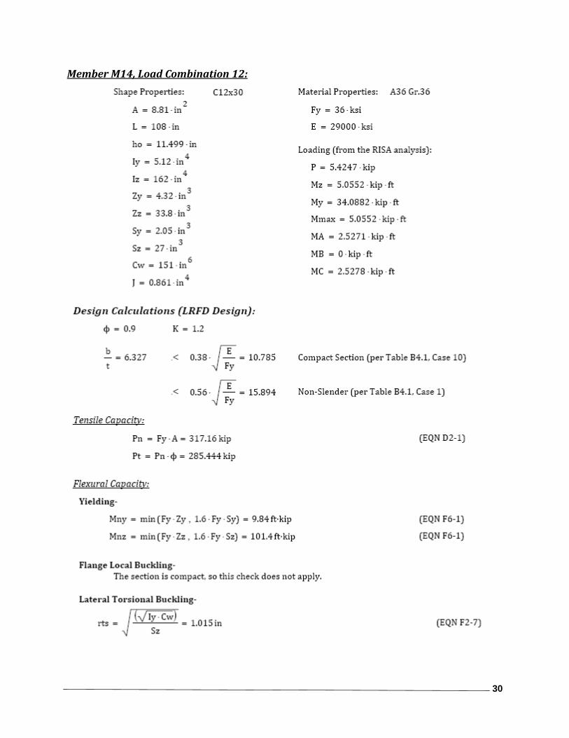
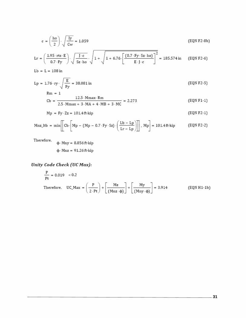
Member M14, Load Combination 12:
31
32
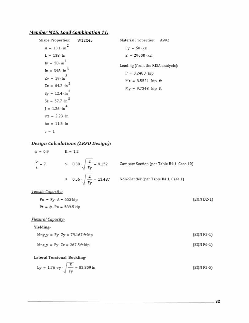
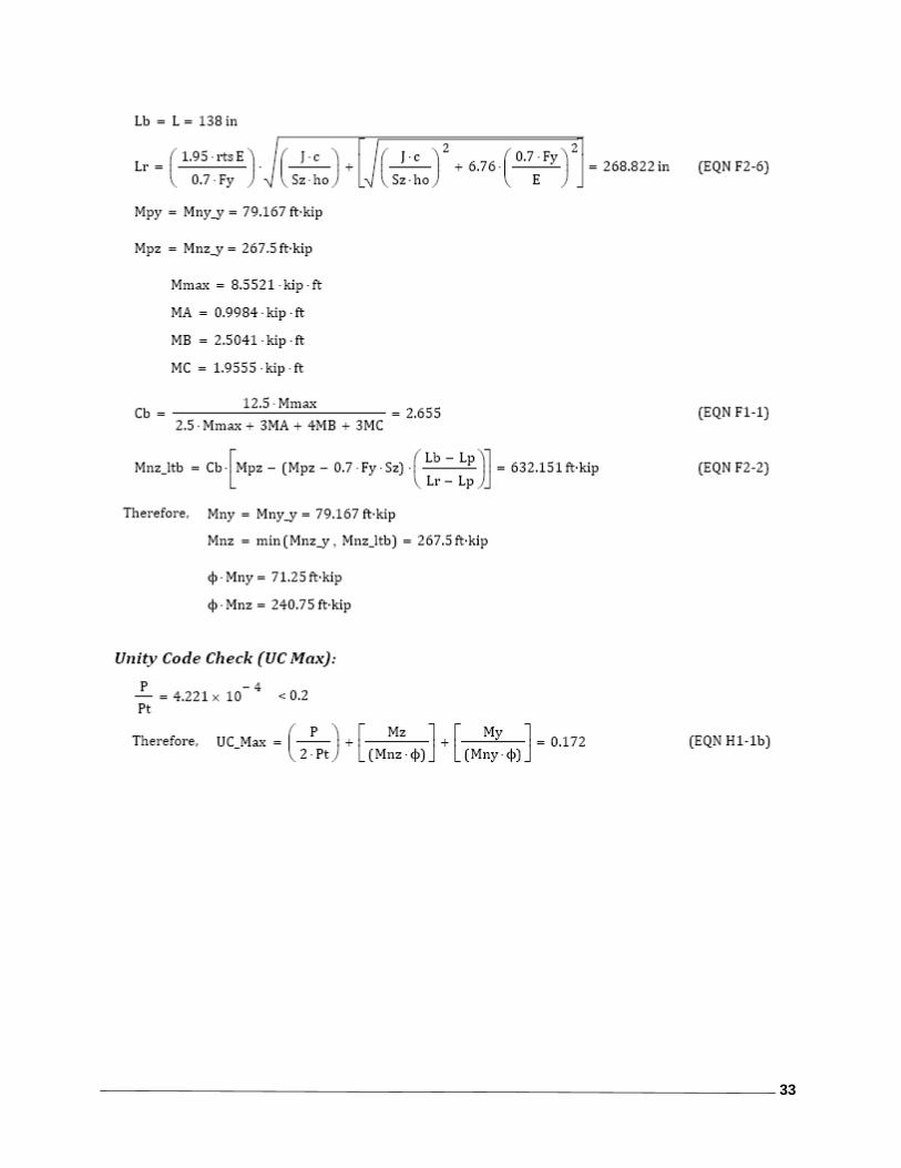
Member M25, Load Combination 11:
33

34
Member M20, Load Combination 13:

35
36
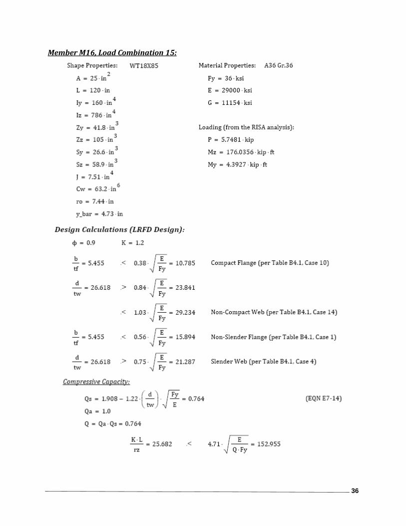
Member M16, Load Combination 15:
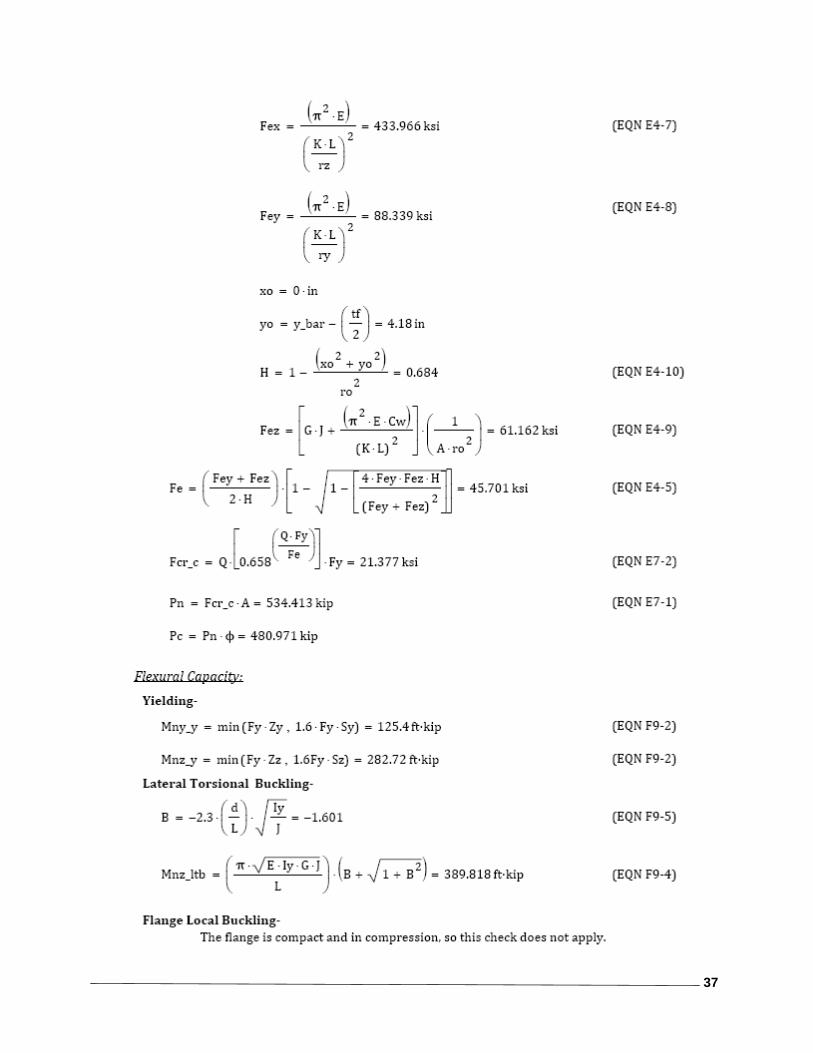
37
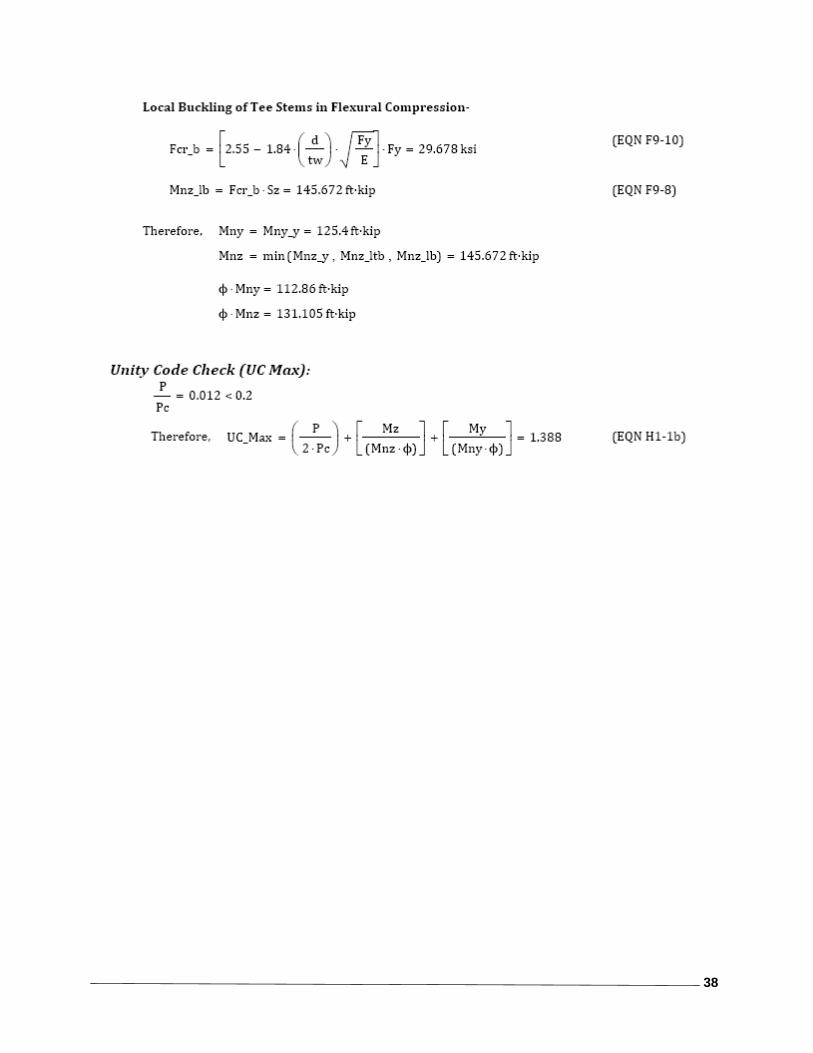
38
39
LRFD Results Comparison
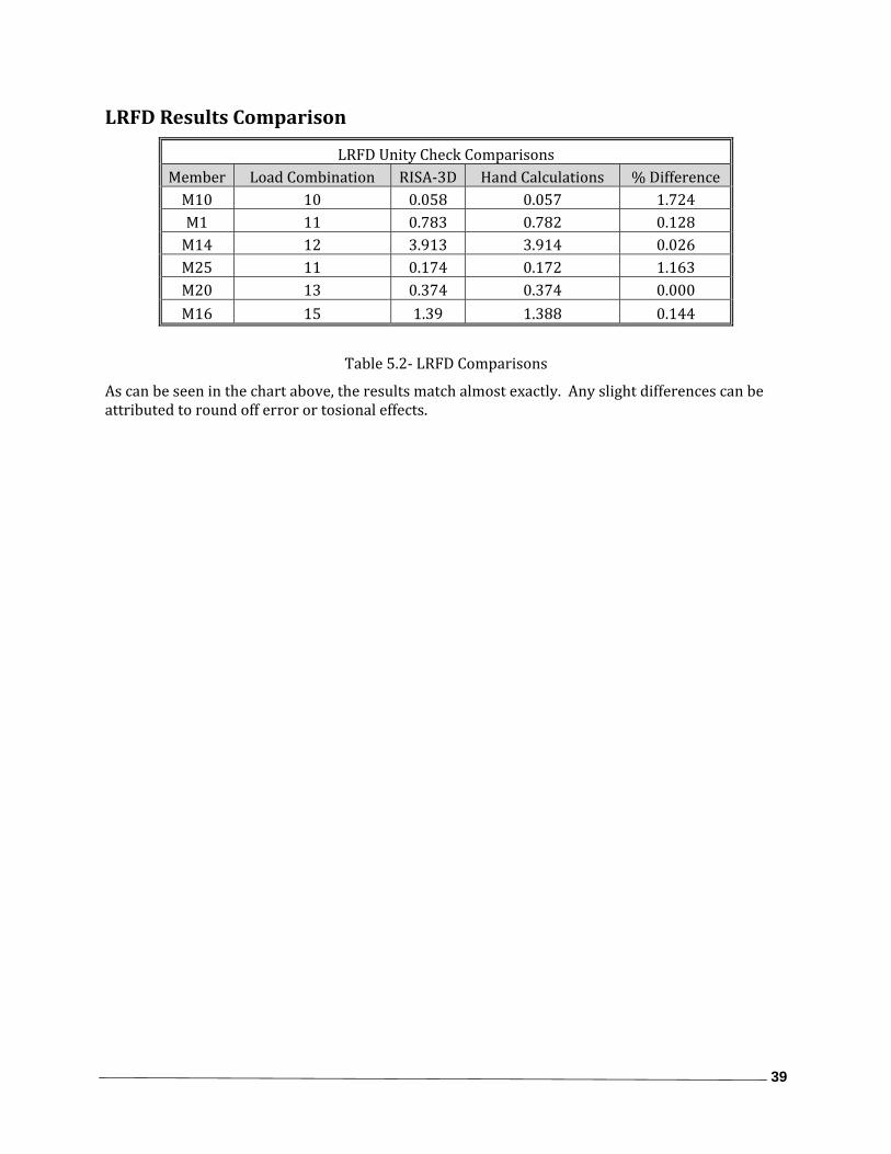
LRFD Unity Check Comparisons Member Load Combination RISA‐3D Hand Calculations % Difference M10 10 0.058 0.057 1.724 M1 11 0.783 0.782 0.128 M14 12 3.913 3.914 0.026 M25 11 0.174 0.172 1.163 M20 13 0.374 0.374 0.000 M16 15 1.39 1.388 0.144
Table 5.2‐ LRFD Comparisons
As can be seen in the chart above, the results match almost exactly. Any slight differences can be attributed to round off error or tosional effects.
40
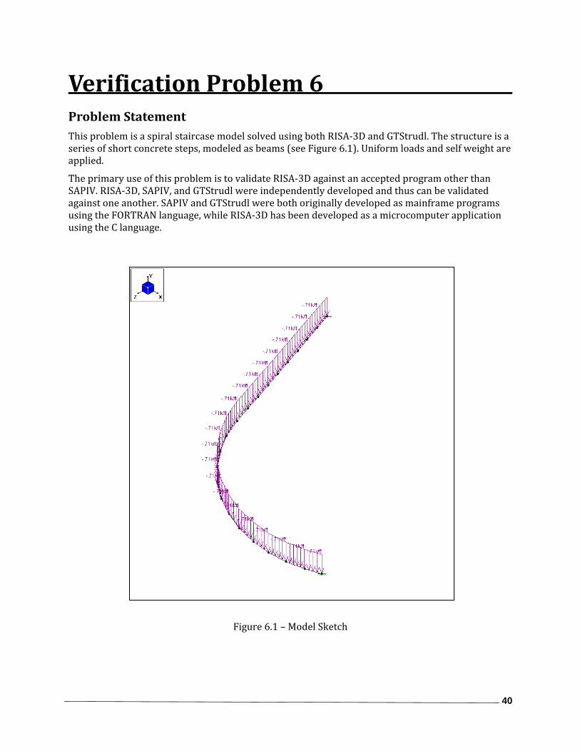
Verification Problem 6 Problem Statement This problem is a spiral staircase model solved using both RISA‐3D and GTStrudl. The structure is a series of short concrete steps, modeled as beams (see Figure 6.1). Uniform loads and self weight are applied.
The primary use of this problem is to validate RISA‐3D against an accepted program other than SAPIV. RISA‐3D, SAPIV, and GTStrudl were independently developed and thus can be validated against one another. SAPIV and GTStrudl were both originally developed as mainframe programs using the FORTRAN language, while RISA‐3D has been developed as a microcomputer application using the C language.
Figure 6.1 – Model Sketch

41
Validation Method The member forces calculated by RISA‐3D are compared with the GTStrudl member forces (see Table 6.1). If the member forces match, it is reasonable to assume the joint displacements also match since the member forces are derived from the joint displacements.
Comparison
Force Comparison: RISA‐3D vs. GTStrudl Member Force RISA‐3D Result GTStrudl Result % Difference
M1 Axial (k) 20.62 20.62 0.000 M5 Y‐Shear (k) 8.94 8.94 0.000 M7 Z‐Shear (k) ‐14.88 ‐14.88 0.000 M10 Torque (k‐ft) ‐0.19 ‐0.19 0.000 M15 My (k‐ft) ‐29.73 ‐29.73 0.000
M18 Mz (k‐ft) 2.14 2.14 0.000
Table 6.1 – Force Comparison
As seen above, the results match exactly.
42
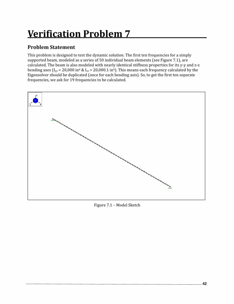
Verification Problem 7 Problem Statement This problem is designed to test the dynamic solution. The first ten frequencies for a simply supported beam, modeled as a series of 50 individual beam elements (see Figure 7.1), are calculated. The beam is also modeled with nearly identical stiffness properties for its y‐y and z‐z bending axes (Iyy = 20,000 in4 & Izz = 20,000.1 in4). This means each frequency calculated by the Eigensolver should be duplicated (once for each bending axis). So, to get the first ten separate frequencies, we ask for 19 frequencies to be calculated.
Figure 7.1 – Model Sketch

43
Validation Method The frequencies calculated by RISA‐3D will be compared to the “exact” frequencies presented by Formulas for Natural Frequency and Mode Shape by Dr. Robert D. Blevins (see Table 7.1).
The equation presented by Blevins for the transverse frequencies is:
Г2
The equation presented by Blevins for the longitudinal frequencies is:
Г2
Where: Г = i*π
m = mass per unit
µ = mass density
i = frequency number (i = 1, 2, 3 . . .)
For our model: E = 30,000 ksi
I = 20,000 in4
m = 0.10783 slugs/in
µ = 0.00074885 slugs/in3
Comparison
Frequency Comparison: RISA‐3D vs. Blevins Frequency
No. Blevins Value
(Hz) RISA‐3D
y‐y Axis Values (Hz)%
DifferenceRISA‐3D
z‐z Axis Values (Hz) %
Difference 1 0.643 0.643 0.003 0.643 0.003 2 2.573 2.573 0.004 2.573 0.004 3 5.790 5.789 0.009 5.789 0.009 4 10.292 10.292 0.004 10.292 0.004 5 16.085 16.082 0.020 16.082 0.020 6 23.158 23.158 0.002 23.158 0.002 7 31.521 31.520 0.004 31.520 0.004 8 41.170 41.168 0.006 41.168 0.005 9 41.699 41.692 0.017 ‐ ‐ 10 52.106 52.101 0.009 52.101 0.009
*Note: Frequency No. 9 is the first longitudinal frequency, it appears only once; it is not duplicated.
Table 7.1 – Frequency Comparison
As can been seen above, the results match almost exactly.

44
Verification Problem 8 Problem Statement This problem is used to test plate/shell elements for bending, membrane action and “twist.” The problem also gives a verification of a rectangular beam member for torsion. The model is of two cantilever beams, the first modeled using a mesh of finite elements, and the second modeled using a rectangular beam (see Figure 8.1). Three different loadings applied at the free ends of the cantilevers are considered. These are an out‐of‐plane bending load, an in‐plane, vertical membrane load, and a torsional twisting moment.
Figure 8.1 – Model Sketch

45
Validation Method This model is validated by comparing the deflections and rotations at the free ends of each cantilever (see Table 8.1). These results will also be checked against theoretical hand calculations. Following are these calculations:
Property Values:
Beam Depth (D) = 60 in
Beam Width (B) = 6 in
Area (A) = 360 in2
Length (L) = 30 ft
Young’s Modulus (E) = 4000 ksi
Shear Modulus (G) = 1539 ksi
Bending load applied at the free end (Pb) = 50 kips
Membrane load applied at the free end (Pm) = 5000 kips
Torsional load applied at the free end (T) = 625 k‐ft (7500 k‐in)
Moment of Inertia for the Bending Load (Ib) = 1080 in4
Moment of Inertia for the Membrane Load (Im) = 108,000 in4
The torsional stiffness (J) is given by:
For: 2a = D = 60 in a = 30 in
2b = B = 6 in b = 3 in
163
3.36 112
4047.8
Therefore, for the given property values:
The free end deflection due to the bending load is:
∆3
12180.038
The free end deflection due to the membrane load is:
∆3
12183.899
The free end rotation due to the torsional load is:
∆ 0.43356
46
Comparison
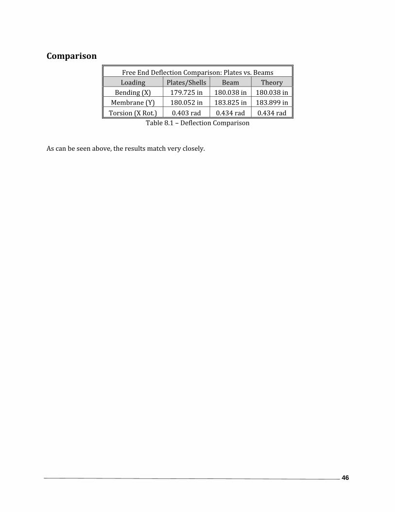
Free End Deflection Comparison: Plates vs. Beams Loading Plates/Shells Beam Theory
Bending (X) 179.725 in 180.038 in 180.038 in Membrane (Y) 180.052 in 183.825 in 183.899 in Torsion (X Rot.) 0.403 rad 0.434 rad 0.434 rad
Table 8.1 – Deflection Comparison
As can be seen above, the results match very closely.
47
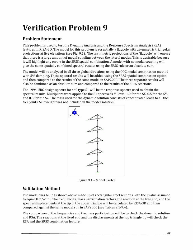
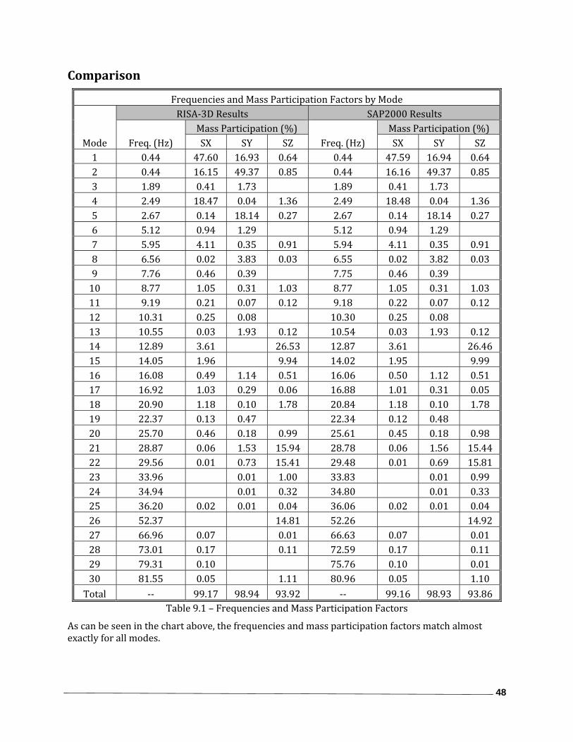
Verification Problem 9 Problem Statement This problem is used to test the Dynamic Analysis and the Response Spectrum Analysis (RSA) features in RISA‐3D. The model for this problem is essentially a flagpole with asymmetric triangular projections at five elevations (see Fig. 9.1). The asymmetric projections of the “flagpole” will ensure that there is a large amount of modal coupling between the lateral modes. This is desirable because it will highlight any errors in the SRSS spatial combination. A model with no modal coupling will give the same spatially combined spectral results using the SRSS rule or an absolute sum.
The model will be analyzed in all three global directions using the CQC modal combination method with 5% damping. These spectral results will be added using the SRSS spatial combination option and then compared to the results of the same model in SAP2000. The three separate results will also be combined as an absolute sum and compared to the results of the SRSS reactions.
The 1994 UBC design spectra for soil type S1 will be the response spectra used to obtain the spectral results. Multipliers were applied to the S1 spectra as follows: 1.0 for the SX, 0.5 for the SY, and 0.3 for the SZ. The mass used for the dynamic solution consists of concentrated loads to all the free joints. Self weight was not included in the model solution.
Figure 9.1 – Model Sketch
Validation Method The model was built as shown above made up of rectangular steel sections with the J value assumed to equal 182.52 in4. The frequencies, mass participation factors, the reaction at the free end, and the spectral displacements at the tip of the upper triangle will be calculated by RISA‐3D and then compared against the same model run in SAP2000 (see Tables 9.1‐9.4).
The comparison of the frequencies and the mass participation will be to check the dynamic solution and RSA. The reactions at the fixed end and the displacements at the top triangle tip will check the RSA and the SRSS combination feature.
48
Comparison
Frequencies and Mass Participation Factors by Mode
Mode
RISA‐3D Results SAP2000 Results
Freq. (Hz) Mass Participation (%)
Freq. (Hz) Mass Participation (%)
SX SY SZ SX SY SZ 1 0.44 47.60 16.93 0.64 0.44 47.59 16.94 0.64 2 0.44 16.15 49.37 0.85 0.44 16.16 49.37 0.85 3 1.89 0.41 1.73 1.89 0.41 1.73 4 2.49 18.47 0.04 1.36 2.49 18.48 0.04 1.36 5 2.67 0.14 18.14 0.27 2.67 0.14 18.14 0.27 6 5.12 0.94 1.29 5.12 0.94 1.29 7 5.95 4.11 0.35 0.91 5.94 4.11 0.35 0.91 8 6.56 0.02 3.83 0.03 6.55 0.02 3.82 0.03 9 7.76 0.46 0.39 7.75 0.46 0.39 10 8.77 1.05 0.31 1.03 8.77 1.05 0.31 1.03 11 9.19 0.21 0.07 0.12 9.18 0.22 0.07 0.12 12 10.31 0.25 0.08 10.30 0.25 0.08 13 10.55 0.03 1.93 0.12 10.54 0.03 1.93 0.12 14 12.89 3.61 26.53 12.87 3.61 26.46 15 14.05 1.96 9.94 14.02 1.95 9.99 16 16.08 0.49 1.14 0.51 16.06 0.50 1.12 0.51 17 16.92 1.03 0.29 0.06 16.88 1.01 0.31 0.05 18 20.90 1.18 0.10 1.78 20.84 1.18 0.10 1.78 19 22.37 0.13 0.47 22.34 0.12 0.48 20 25.70 0.46 0.18 0.99 25.61 0.45 0.18 0.98 21 28.87 0.06 1.53 15.94 28.78 0.06 1.56 15.44 22 29.56 0.01 0.73 15.41 29.48 0.01 0.69 15.81 23 33.96 0.01 1.00 33.83 0.01 0.99 24 34.94 0.01 0.32 34.80 0.01 0.33 25 36.20 0.02 0.01 0.04 36.06 0.02 0.01 0.04 26 52.37 14.81 52.26 14.92 27 66.96 0.07 0.01 66.63 0.07 0.01 28 73.01 0.17 0.11 72.59 0.17 0.11 29 79.31 0.10 75.76 0.10 0.01 30 81.55 0.05 1.11 80.96 0.05 1.10 Total ‐‐ 99.17 98.94 93.92 ‐‐ 99.16 98.93 93.86
Table 9.1 – Frequencies and Mass Participation Factors
As can be seen in the chart above, the frequencies and mass participation factors match almost exactly for all modes.
49
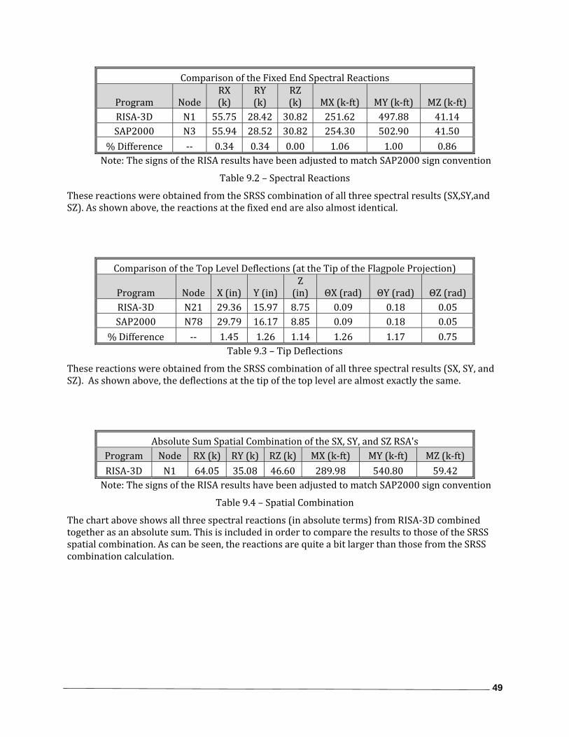
Comparison of the Fixed End Spectral Reactions
Program Node RX (k)
RY (k)
RZ (k) MX (k‐ft) MY (k‐ft) MZ (k‐ft)
RISA‐3D N1 55.75 28.42 30.82 251.62 497.88 41.14 SAP2000 N3 55.94 28.52 30.82 254.30 502.90 41.50
% Difference ‐‐ 0.34 0.34 0.00 1.06 1.00 0.86 Note: The signs of the RISA results have been adjusted to match SAP2000 sign convention
Table 9.2 – Spectral Reactions
These reactions were obtained from the SRSS combination of all three spectral results (SX,SY,and SZ). As shown above, the reactions at the fixed end are also almost identical.
Comparison of the Top Level Deflections (at the Tip of the Flagpole Projection)
Program Node X (in) Y (in) Z (in) ΘX (rad) ΘY (rad) ΘZ (rad)
RISA‐3D N21 29.36 15.97 8.75 0.09 0.18 0.05 SAP2000 N78 29.79 16.17 8.85 0.09 0.18 0.05
% Difference ‐‐ 1.45 1.26 1.14 1.26 1.17 0.75 Table 9.3 – Tip Deflections
These reactions were obtained from the SRSS combination of all three spectral results (SX, SY, and SZ). As shown above, the deflections at the tip of the top level are almost exactly the same.
Absolute Sum Spatial Combination of the SX, SY, and SZ RSA's Program Node RX (k) RY (k) RZ (k) MX (k‐ft) MY (k‐ft) MZ (k‐ft) RISA‐3D N1 64.05 35.08 46.60 289.98 540.80 59.42 Note: The signs of the RISA results have been adjusted to match SAP2000 sign convention
Table 9.4 – Spatial Combination
The chart above shows all three spectral reactions (in absolute terms) from RISA‐3D combined together as an absolute sum. This is included in order to compare the results to those of the SRSS spatial combination. As can be seen, the reactions are quite a bit larger than those from the SRSS combination calculation.
50
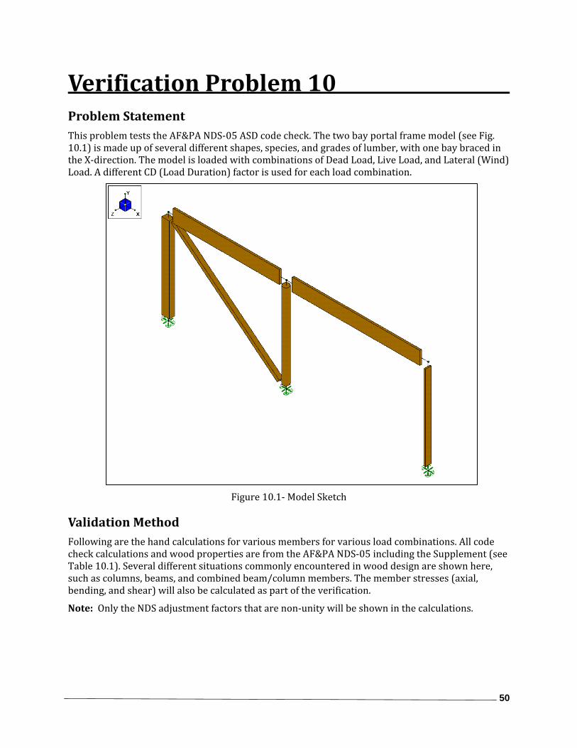
Verification Problem 10 Problem Statement This problem tests the AF&PA NDS‐05 ASD code check. The two bay portal frame model (see Fig. 10.1) is made up of several different shapes, species, and grades of lumber, with one bay braced in the X‐direction. The model is loaded with combinations of Dead Load, Live Load, and Lateral (Wind) Load. A different CD (Load Duration) factor is used for each load combination.
Figure 10.1‐ Model Sketch
Validation Method Following are the hand calculations for various members for various load combinations. All code check calculations and wood properties are from the AF&PA NDS‐05 including the Supplement (see Table 10.1). Several different situations commonly encountered in wood design are shown here, such as columns, beams, and combined beam/column members. The member stresses (axial, bending, and shear) will also be calculated as part of the verification.
Note: Only the NDS adjustment factors that are non‐unity will be shown in the calculations.

51
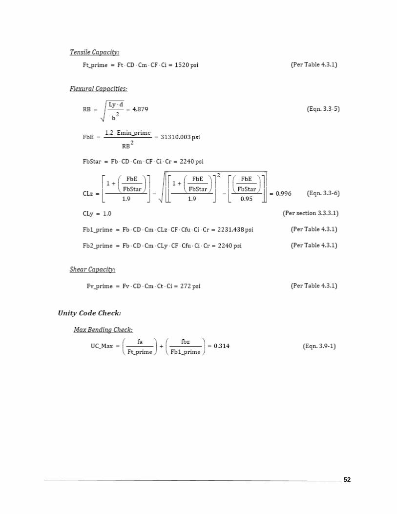
Member M1, Load Combo 3: (DL +LL+Wind)
52
53
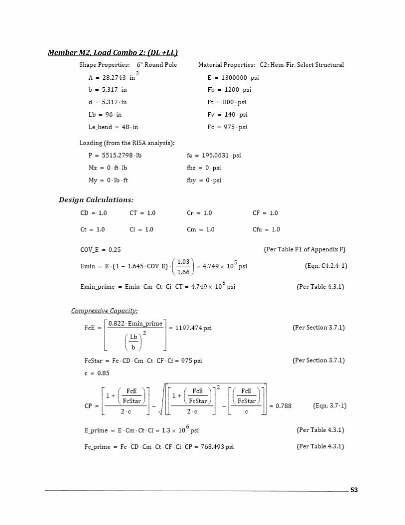
Member M2, Load Combo 2: (DL +LL)

54
*Note: For some members the limitations in section 3.6.3 control over any of the equations. This is because in the Compression‐Bending Interaction equation (Eqn. 3.9‐3), if the bending goes to zero, the equation will automatically square the compression portion, lowering it from what we know to be the actual capacity ( fc/Fc’ vs. (fc/Fc’)2 ). This section allows us to use the compression portion without squaring it to know the true capacity of the compression‐only member.
55
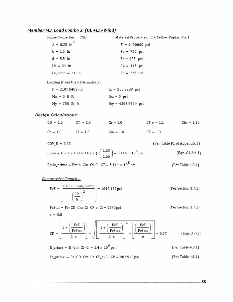
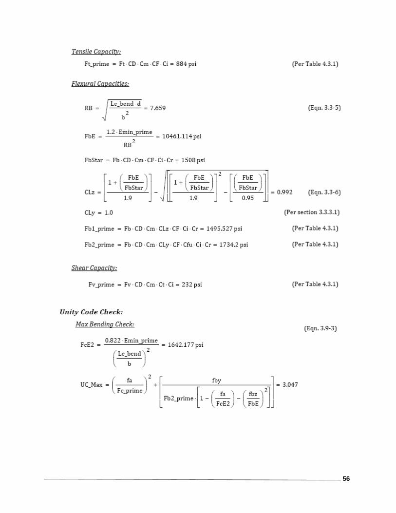
Member M3, Load Combo 3: (DL +LL+Wind)
56
57
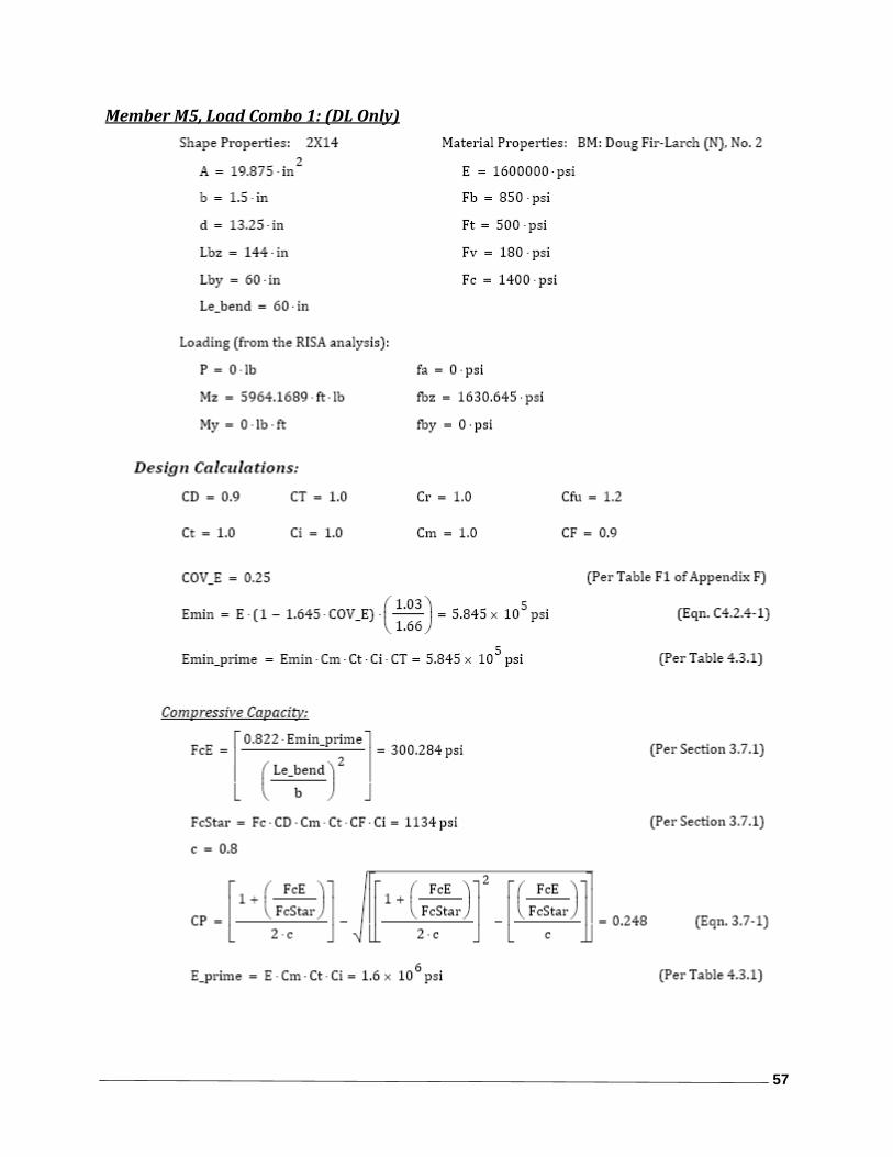
Member M5, Load Combo 1: (DL Only)

58
59
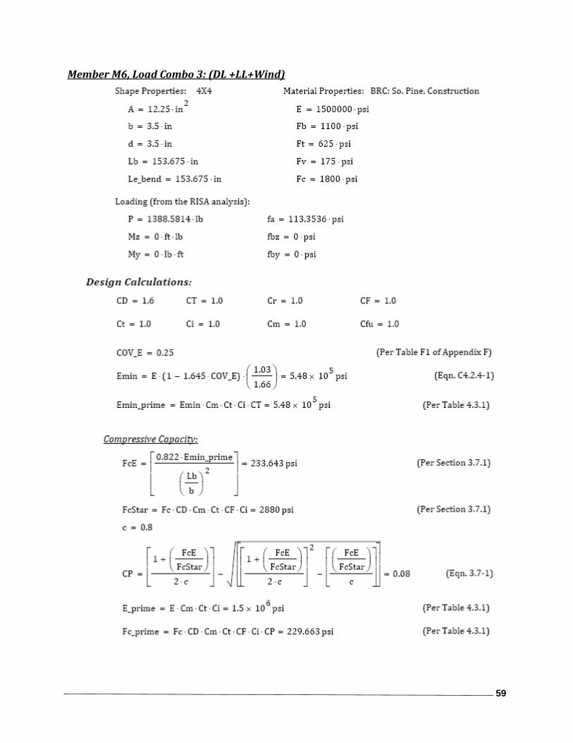
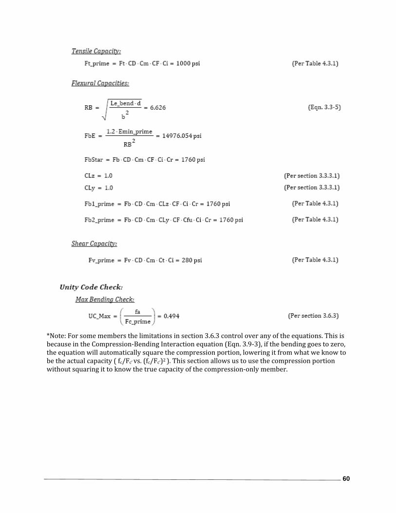
Member M6, Load Combo 3: (DL +LL+Wind)
60
*Note: For some members the limitations in section 3.6.3 control over any of the equations. This is because in the Compression‐Bending Interaction equation (Eqn. 3.9‐3), if the bending goes to zero, the equation will automatically square the compression portion, lowering it from what we know to be the actual capacity ( fc/Fc’ vs. (fc/Fc’)2 ). This section allows us to use the compression portion without squaring it to know the true capacity of the compression‐only member.
61
Comparison
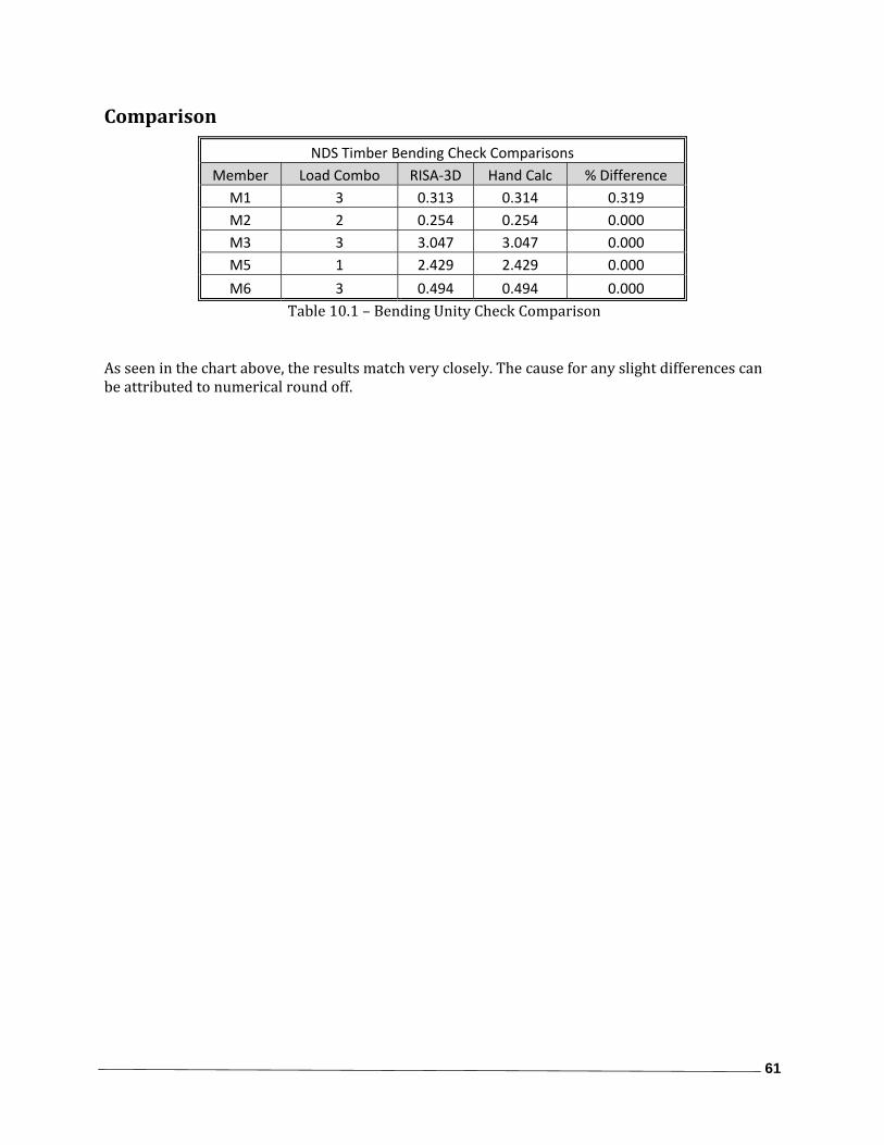
NDS Timber Bending Check Comparisons Member Load Combo RISA‐3D Hand Calc % Difference
M1 3 0.313 0.314 0.319 M2 2 0.254 0.254 0.000 M3 3 3.047 3.047 0.000 M5 1 2.429 2.429 0.000
M6 3 0.494 0.494 0.000 Table 10.1 – Bending Unity Check Comparison
As seen in the chart above, the results match very closely. The cause for any slight differences can be attributed to numerical round off.

62
Verification Problem 11 Problem Statement This problem is used to test the tapered WF sections. A typical single bay with a sloped roof (see Fig. 11.1) will be analyzed using tapered WF sections for the columns and beams. Loading will consist of vertical member projected loads, lateral member distributed loads, and member point loads. Gravity self weight will also be applied.
Figure 11.1‐ Model Sketch of Frames
Validation Method The frame analyzed with tapered WF sections will be compared to a similar frame, which is modeled with 14 piecewise prismatic sections for each tapered WF member in the original frame (see Fig. 11.1). Since each tapered WF member is modeled internally as a 14 piecewise prismatic “member,” the results should match very closely. Selected joint deflections, reactions, and member section forces will be compared (see Tables 11.1‐11.3). The ASD code checks on the tapered WF sections (for member properties see Table 11.4) will be compared to hand calculations using the ASD 9th Ed. Steel Code.
Note: This problem uses the AISC 9th Ed. because the AISC 13th Ed. and 14th Ed. Steel Codes do not include provisions for code check equations for tapered members.

63
Comparison
Comparison of Joint Deflections Tapered WF Frame Equivalent "Piecewise" Frame
Node Direction Deflection (in) Node Direction Deflection (in) N2 X ‐0.8769 N7 X ‐0.8769 N3 Y ‐3.0016 N8 Y ‐3.0017 N4 X 0.2897 N9 X 0.2896
Table 11.1 – Joint Deflections
The joint deflections were checked at the top left corner, peak, and top right corner, respectively. As is seen in the chart above, the results match almost exactly.
Comparison of Base Reactions Tapered WF Frame Equivalent "Piecewise" Frame
Node X (k) Y (k) MZ (k‐ft) Node X (k) Y (k) MZ (k‐ft) N1 5.659 18.533 0 N6 5.659 18.533 0 N5 ‐10.859 17.091 41.749 N10 ‐10.859 17.091 41.750
Table 11.2 – Base Reactions
The reactions were checked at the two base nodes. As seen above, the results match almost exactly.
Comparison of Member Section Forces Tapered WF Frame Equivalent "Piecewise" Frame
Member Section Cut Location Local
DirectionValue
(k, or k‐ft) Member Section Cut Location
Local Direction
Value (k, or k‐ft)
M1 5 Mz 108.6293 M18 5 Mz 108.6308M1 1 x 18.5332 M5 1 x 18.5332 M2 5 y ‐15.9157 M32 5 y ‐15.9139M2 5 Mz 108.6283 M32 5 Mz 108.6308M2 1 Mz ‐30.9719 M19 1 Mz ‐30.9701M3 1 Mz ‐30.9719 M47 1 Mz ‐30.9701M3 5 Mz 99.7789 M60 5 Mz 99.7812 M3 5 y ‐14.5012 M60 5 y ‐14.4995M4 5 Mz ‐99.7799 M46 5 Mz ‐99.7812M4 1 x 17.0907 M33 1 x 17.0907
Table 11.3 – Member Forces
The section forces were checked at the base of the columns, at the corner joints, and at the peak. As can be seen in the chart above, the results match almost exactly.
64
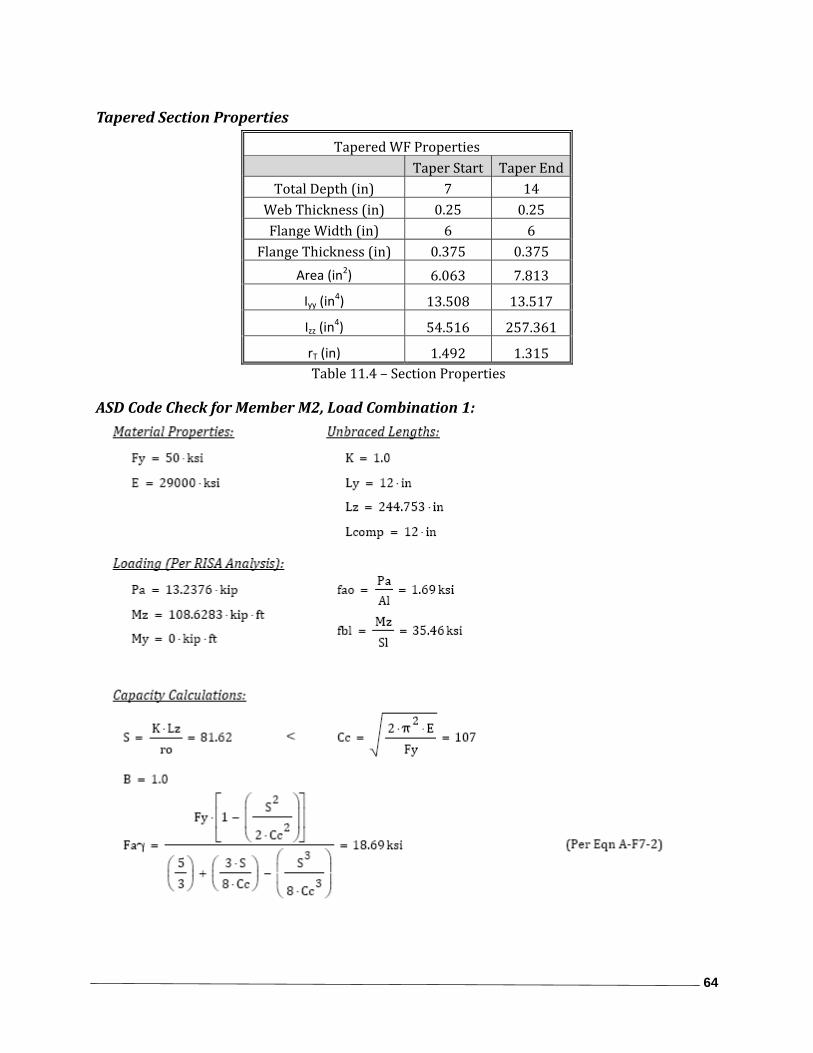
Tapered Section Properties
Tapered WF Properties Taper Start Taper End
Total Depth (in) 7 14 Web Thickness (in) 0.25 0.25 Flange Width (in) 6 6
Flange Thickness (in) 0.375 0.375 Area (in2) 6.063 7.813
Iyy (in4) 13.508 13.517
Izz (in4) 54.516 257.361
rT (in) 1.492 1.315 Table 11.4 – Section Properties
ASD Code Check for Member M2, Load Combination 1:
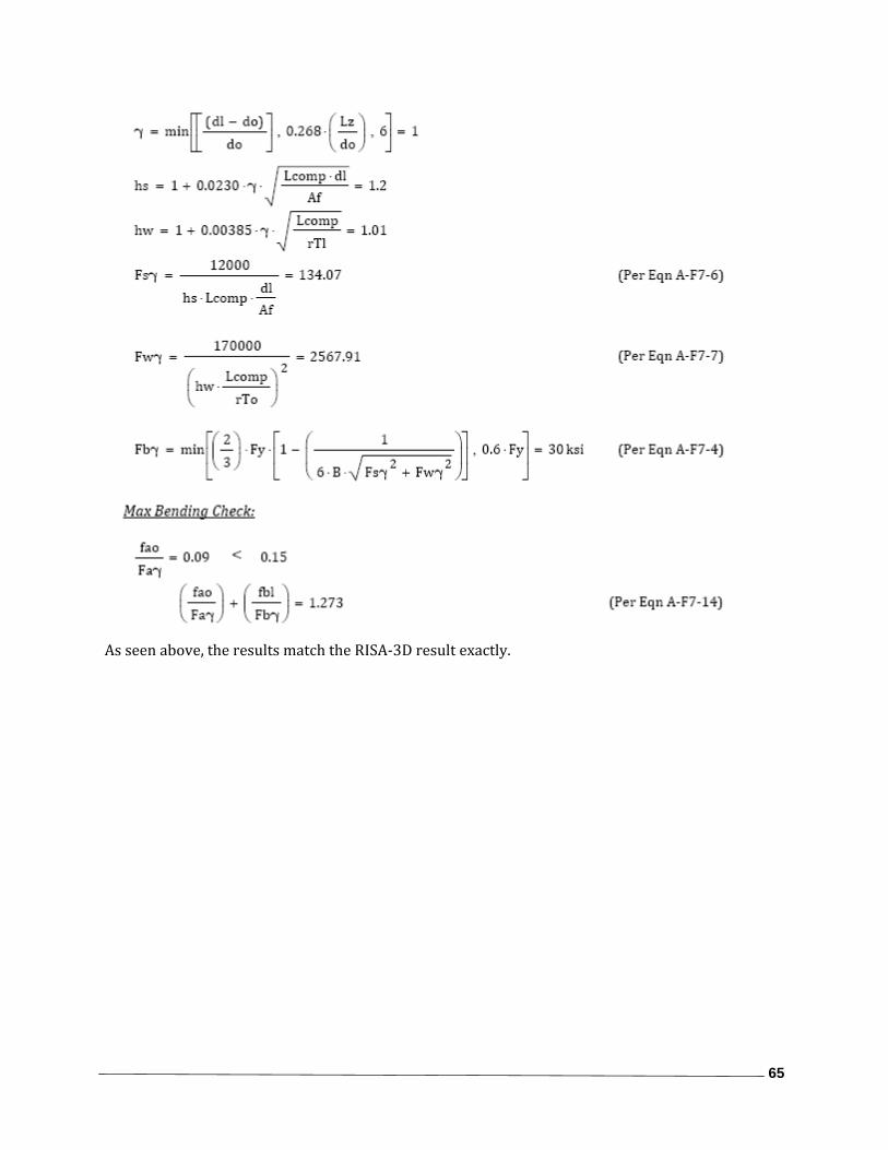
65
As seen above, the results match the RISA‐3D result exactly.
66
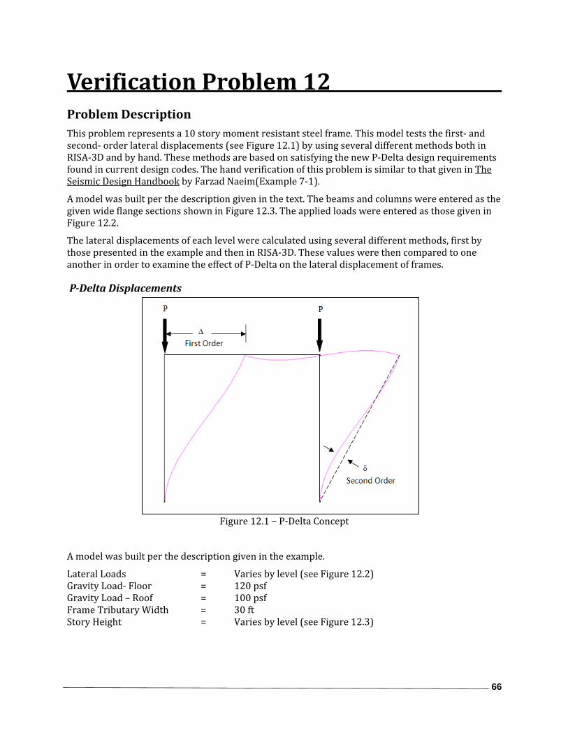
Verification Problem 12 Problem Description This problem represents a 10 story moment resistant steel frame. This model tests the first‐ and second‐ order lateral displacements (see Figure 12.1) by using several different methods both in RISA‐3D and by hand. These methods are based on satisfying the new P‐Delta design requirements found in current design codes. The hand verification of this problem is similar to that given in The Seismic Design Handbook by Farzad Naeim(Example 7‐1).
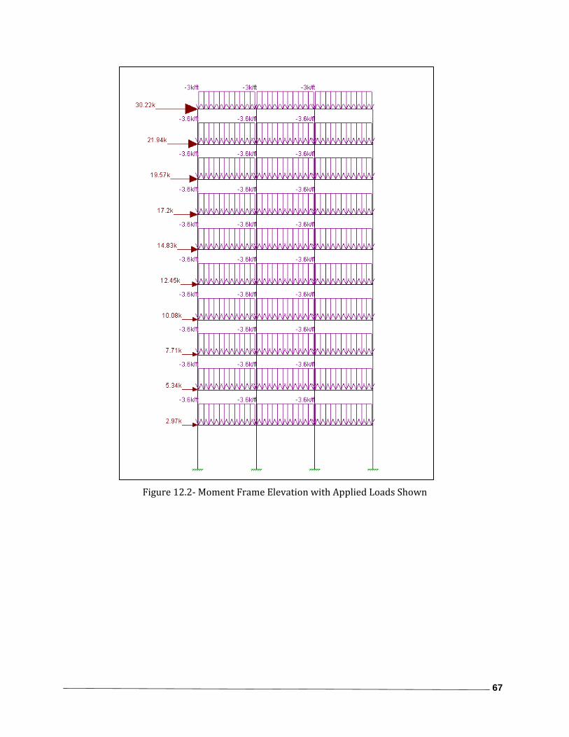
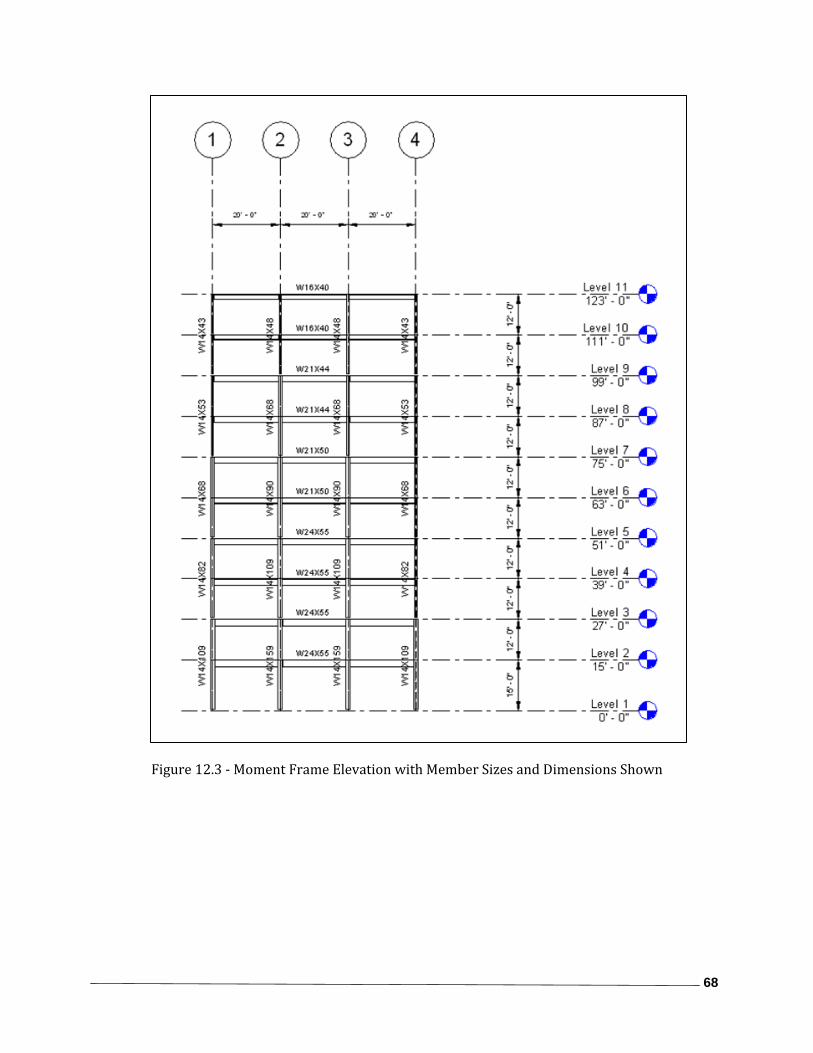
A model was built per the description given in the text. The beams and columns were entered as the given wide flange sections shown in Figure 12.3. The applied loads were entered as those given in Figure 12.2.
The lateral displacements of each level were calculated using several different methods, first by those presented in the example and then in RISA‐3D. These values were then compared to one another in order to examine the effect of P‐Delta on the lateral displacement of frames.
PDelta Displacements
Figure 12.1 – P‐Delta Concept
A model was built per the description given in the example.
Lateral Loads = Varies by level (see Figure 12.2) Gravity Load‐ Floor = 120 psf Gravity Load – Roof = 100 psf Frame Tributary Width = 30 ft Story Height = Varies by level (see Figure 12.3)
67
Figure 12.2‐ Moment Frame Elevation with Applied Loads Shown
68
Figure 12.3 ‐ Moment Frame Elevation with Member Sizes and Dimensions Shown

69
Validation Method
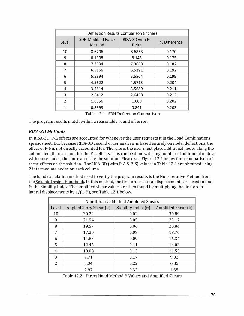
SDH Methods The Seismic Design Handbook utilizes two methods for analyzing the second order P‐delta effects. The first is an iterative process where an analytical model is first used to compute the first order displacements from the applied loads. These displacements are then re‐applied to the model as secondary shears giving the user a modified set of displacements. This process is repeated until a reasonable convergence of data produces the final lateral displacement. See Table 12.2 for a comparison of these deflections versus those of the RISA‐3D P‐Delta feature, below.
The second method, the Non‐Iterative P‐delta Method, is a hand calculated simplification of the iterative method. Using the assumption that story drift at any level is proportional only to the applied story shear at that level, the first order deflections are calculated using an applied lateral load and then multiplied by a magnification factor to account for the second order P‐delta effects.
Note: Because the example calculation does not account for axial shortening of the columns, the elastic analysis in their methods differs by up to 2% from that of other methods outlined in this example.
SDH Comparison The graph (Figure 12.3) below shows the minimal difference between the SDH Methods.
Figure 12.3 ‐ Comparison of Deflections from each SDH Method
70
Deflection Results Comparison (inches)
Level SDH Modified Force
Method RISA‐3D with P‐
Delta % Difference
10 8.6706 8.6853 0.170 9 8.1308 8.145 0.175 8 7.3534 7.3668 0.182 7 6.5166 6.5291 0.192 6 5.5394 5.5504 0.199 5 4.5622 4.5715 0.204 4 3.5614 3.5689 0.211 3 2.6412 2.6468 0.212 2 1.6856 1.689 0.202
1 0.8393 0.841 0.203 Table 12.1– SDH Deflection Comparison
The program results match within a reasonable round off error.
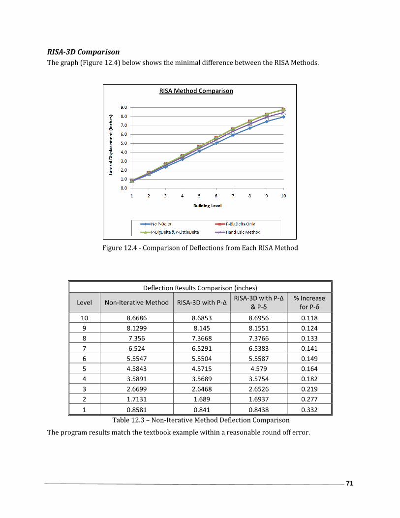
RISA3D Methods In RISA‐3D, P‐∆ effects are accounted for whenever the user requests it in the Load Combinations spreadsheet. But because RISA‐3D second order analysis is based entirely on nodal deflections, the effect of P‐δ is not directly accounted for. Therefore, the user must place additional nodes along the column length to account for the P‐δ effects. This can be done with any number of additional nodes; with more nodes, the more accurate the solution. Please see Figure 12.4 below for a comparison of these effects on the solution. TheRISA‐3D (with P‐∆ & P‐δ) values in Table 12.3 are obtained using 2 intermediate nodes on each column.
The hand calculation method used to verify the program results is the Non‐Iterative Method from the Seismic Design Handbook. In this method, the first order lateral displacements are used to find Ѳ, the Stability Index. The amplified shear values are then found by multiplying the first order lateral displacements by 1/(1‐Ѳ), see Table 12.1 below.
Non‐Iterative Method Amplified Shears Level Applied Story Shear (k) Stability Index (θ) Amplified Shear (k) 10 30.22 0.02 30.89 9 21.94 0.05 23.12 8 19.57 0.06 20.84 7 17.20 0.08 18.70 6 14.83 0.09 16.34 5 12.45 0.11 14.03 4 10.08 0.13 11.55 3 7.71 0.17 9.32 2 5.34 0.22 6.85 1 2.97 0.32 4.35
Table 12.2 ‐ Direct Hand Method Ѳ Values and Amplified Shears
71
RISA3D Comparison The graph (Figure 12.4) below shows the minimal difference between the RISA Methods.
Figure 12.4 ‐ Comparison of Deflections from Each RISA Method
Deflection Results Comparison (inches)
Level Non‐Iterative Method RISA‐3D with P‐∆ RISA‐3D with P‐∆
& P‐δ % Increase for P‐δ
10 8.6686 8.6853 8.6956 0.118 9 8.1299 8.145 8.1551 0.124 8 7.356 7.3668 7.3766 0.133 7 6.524 6.5291 6.5383 0.141 6 5.5547 5.5504 5.5587 0.149 5 4.5843 4.5715 4.579 0.164 4 3.5891 3.5689 3.5754 0.182 3 2.6699 2.6468 2.6526 0.219 2 1.7131 1.689 1.6937 0.277
1 0.8581 0.841 0.8438 0.332 Table 12.3 – Non‐Iterative Method Deflection Comparison
The program results match the textbook example within a reasonable round off error.
72
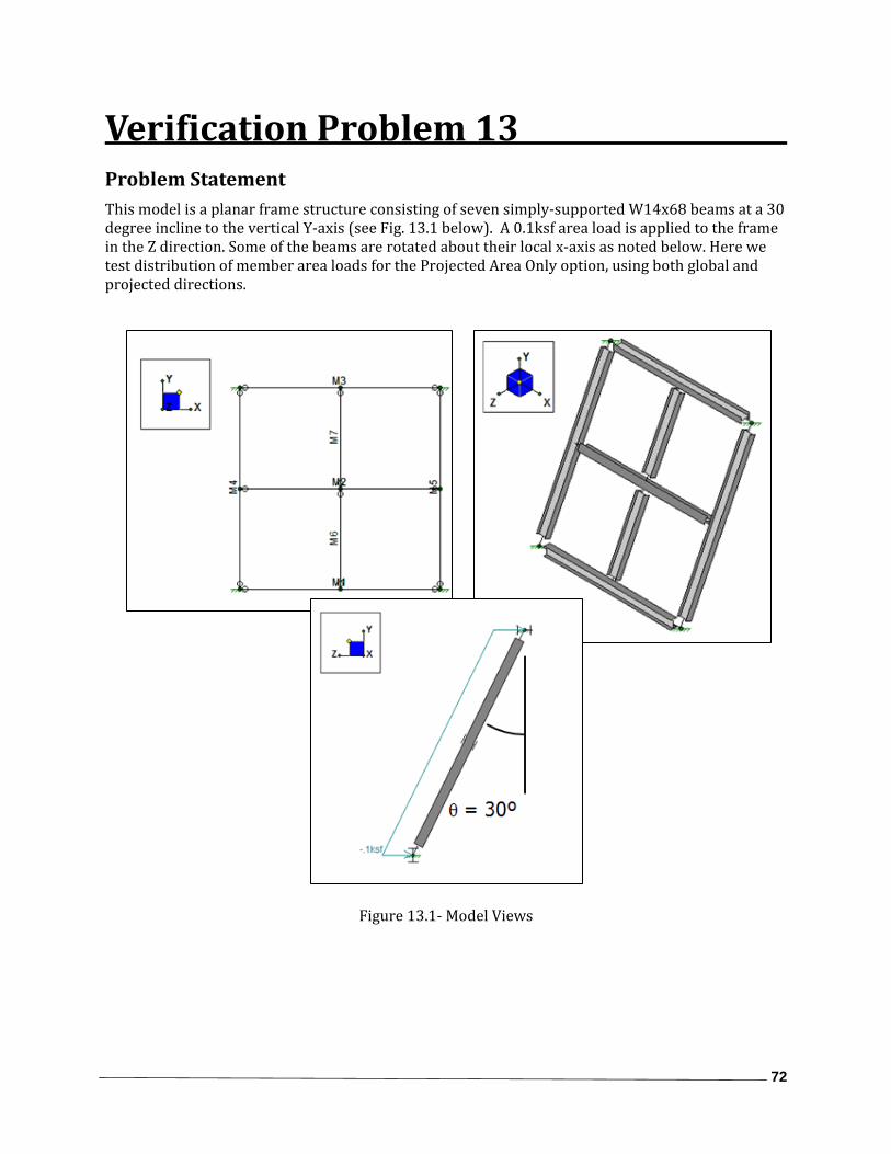
Verification Problem 13 Problem Statement This model is a planar frame structure consisting of seven simply‐supported W14x68 beams at a 30 degree incline to the vertical Y‐axis (see Fig. 13.1 below). A 0.1ksf area load is applied to the frame in the Z direction. Some of the beams are rotated about their local x‐axis as noted below. Here we test distribution of member area loads for the Projected Area Only option, using both global and projected directions.
Figure 13.1‐ Model Views

73
Validation Method Envelope dimensions of the projected sections are used to calculate equivalent uniform member distributed loads. The projected section depth and width:
Equivalent uniform member distributed loads can then be calculated for both the global Z and H (projected Z) directions:
Where θ = vertical angle [deg.]
φ = local axis rotation angle [deg.]
d =total section depth [in.]
bf =total section width [in.]
dprojected = projected section depth [in.]
ω = equivalent uniform member distributed load [k/ft]
ρ = uniform member area load [k/ft]
Comparison For this model:
W14X68 d = 14.04 in. bf = 10.035 in.
Equivalent Uniform Member Distributed Loads, ωZ
Member θ φ Global Z (k/ft) Projected Z (k/ft)
deg. deg. Theoretical RISA‐3D %Diff. Theoretical RISA‐3D %Diff. M1 90 0 0.135 0.135 0.00 0.117 0.117 0.00 M2 90 60 0.151 0.151 0.00 0.131 0.131 0.00
M3 90 90 0.097 0.096 1.03 0.084 0.083 1.19 Table 13.1 – Load Calculation Comparison
As seen in Table 13.1 above, the results match exactly.
74
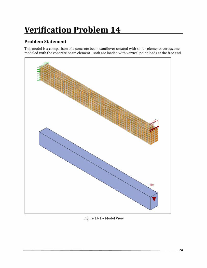
Verification Problem 14 Problem Statement This model is a comparison of a concrete beam cantilever created with solids elements versus one modeled with the concrete beam element. Both are loaded with vertical point loads at the free end.
Figure 14.1 – Model View

75
Validation Method The deflections at the tip of each cantilever are compared to the values obtained by hand calculations. Deflection at the tip of a cantilever beam is calculated as follows:
∆3
Where,
P = 10 kips
L = 10 ft = 120 in
E = 3644 ksi (Conc4NW material)
I = 1152 in4
Therefore, per our hand calculation, ∆ 1.372 .
Comparison For this model:
Beam Deflection Comparison
Element Node RISA‐3D Bending Deflection (in) % Difference
Solids N1115 ‐1.361 0.80 Beam N2137 ‐1.372 0.00
Table 14.1 – Load Calculation Comparison
As seen in Table 14.1 above, the results are within a reasonable difference from the hand calculations.