3D shape recognition and reconstruction based on line element geometry

M. Hofer, B. Odehnal, H. Pottmann, T. Steiner, J. WallnerInstitute of Discrete Mathematics and Geometry, TU Wien

{hofer,odehnal,pottmann,tsteiner,wallner}@geometrie.tuwien.ac.at

Abstract

This paper presents a new method for the recognitionand reconstruction of surfaces from 3D data. Line elementgeometry, which generalizes both line geometry and the La-guerre geometry of oriented planes, enables us to recog-nize a wide class of surfaces (spiral surfaces, cones, heli-cal surfaces, rotational surfaces, cylinders, etc.) by fittinglinear subspaces in an appropriate seven-dimensional im-age space. In combination with standard techniques suchas PCA and RANSAC, line element geometry is employedto effectively perform the segmentation of complex objectsaccording to surface type. Examples show applications inreverse engineering of CAD models and testing mathemat-ical hypotheses concerning the exponential growth of seashells.

1. Introduction

Computer Vision has adopted and extended a variety ofmethods from geometry (see e.g. [1, 4]). Even such a spe-cialized field as line geometry has recently received atten-tion in connection with generalized cameras [14, 26] and 3Dshape understanding and surface reconstruction [3, 18, 17].The latter topic has also been addressed with Gaussian im-age methods [21], the extended Gaussian image [6] and theLaguerre geometry of oriented planes [15].

The present paper introduces the geometry of orientedline elements – a line element consisting of a line and a pointon it. From the structural viewpoint, line element geometryis a unifying theory for the geometry of both oriented linesand oriented planes. Mainly however it is a new tool for 3Dshape understanding and reconstruction capable of solvingproblems which previous approaches could not handle.

This paper deals with surface-like point clouds and trian-gle meshes. The link to line element geometry is providedby the surface normals – we assume that we can obtain adiscrete number of points on the surface and estimate sur-face normals there (see e.g. [21]; modern 3D photography

This work was supported by the Austrian Science Fund(FWF) under grant No. S9206.

and corresponding software actually deliver data points plusnormals).

Previous Work. We are interested in the recognition andreconstruction of special surface types and in the segmen-tation of a 3D data set according to these types. Thus welimit our brief literature review to these topics. In ComputerVision, recognition and reconstruction of special shapes isoften performed by methods related to the Hough transform(see e.g. [7, 10]). Pure Hough transform methods work in‘spaces of shapes’ and quickly lead to high dimensions andreduced efficiency. They have therefore been augmentedby geometric constructions like the Gaussian image of dif-ferential geometry [21]. Because that is constructed solelyfrom normal vectors, it is unable to distinguish, for exam-ple, between parallel planes. Both the extended Gaussianimage [6] and the geometry of oriented planes [15] are im-provements and work excellent for the detection of spheresand developable surfaces. They cannot, however, easily de-tect rotational or helical surfaces, which in turn are handlednicely by line geometry [3, 18, 17].

We understand all these methods as local shape detec-tors. Their beauty lies in the fact that after introducingappropriate coordinates for the various geometric objectsassociated with the original data, shape understanding andreconstruction is reduced to the simple problem of fittinglinear subspaces to point cloud data. Both principal compo-nent analysis (PCA) and the RANSAC principle [4] can ef-fectively be employed. Even if such a method does not leadto an optimal fit of the original data with a special surface(e.g. due to noise), the results are still useful for initializingnonlinear optimization procedures [21, 24].

The result of a local shape detector may be seen as alabeled image (with N colors) defined on a surface. Forfurther processing, especially surface segmentation, regiongrowing algorithms [21] and other methods of mathemati-cal morphology [5, 11, 19, 22] have been applied. In or-der to make region growing procedures stop at feature re-gions such as sharp edges or blended edges, Pottmann et al.[16] uses a metric which incorporates the surface normalsas well. Their approach is a special case of an image man-ifold in the sense of Kimmel, Malladi and Sochen [9], and

PSfrag replacements

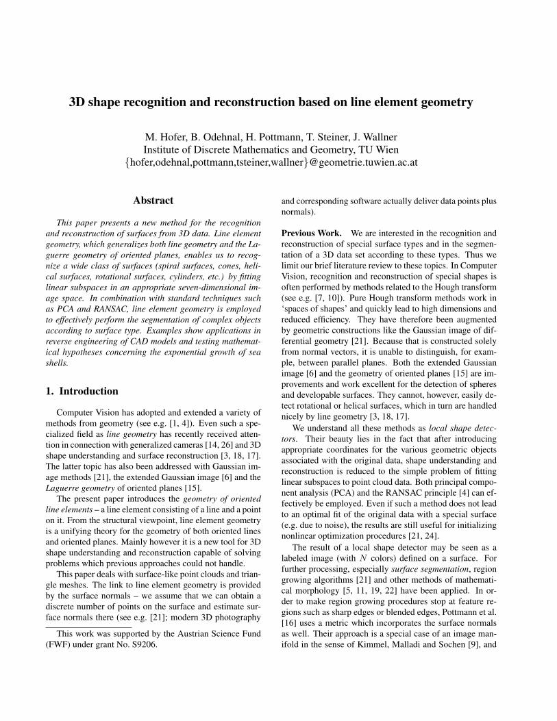
l = x× ll

L

λ x

ol × l

Figure 1. Coordinates (l, l, λ) for a line element.

is closely related to line element geometry.

Contributions of the present paper. The main contribu-tion of the present paper is to introduce line element geome-try for use in 3D shape recognition and reconstruction. Lineelement geometry does not appear in the classical geometricliterature, despite its close relation to well studied subjectssuch as line geometry, Laguerre geometry, equiform kine-matics [8] and spiral surfaces [25].

Our paper is organized as follows: We present the basicsof line element geometry and its relation to equiform kine-matics in Sec. 2. Sec. 3 shows how surface normal elementsassociated with the input data are used to detect a varietyof special surface types. A segmentation algorithm is dis-cussed in Sec. 4. Sec. 5 illustrates our algorithms by meansof data obtained from nature and by reverse engineering of3D technical objects.

2. The Manifold of Line Elements

A line element consists of a line L in R3 and a point xon it. We endow L with an orientation, which means thatwe choose one of the two unit vectors parallel to L. Linegeometry [18] coordinatizes an oriented line by normalizedPlucker coordinates (l, l), where l is the unit vector parallelto L, and l := x × l is the momentum vector of the line. ldoes not depend on the choice of x on L and has the prop-erty that l · l = 0. L is recovered from (l, l) as the solutionset of the 3 linear equations l = x× l. A 7-th coordinate isneeded in order to locate a point x on L: we add λ := x · lto the standard Plucker coordinates, thus representing a lineelement by (l, l, λ). It is elementary that x = l × l + λl(see Fig. 1). The coordinate vector (l, l, λ) is a point of R7.Conversely it is not difficult to show that (l, l, λ) ∈ R7 rep-resents a line element if and only if l · l = 1 and l · l = 0.

Normal elements and Laguerre geometry. Each point xof the surface Φ of a 3D volume has an outward unit normalvector n, if Φ is smooth. Thus a normal line element at xis defined, whose coordinates are (n, x × n, x · n). In thisway a surface Φ in R3 has an associated surface Γ(Φ) inR7, which consists of the normal line elements of Φ. Wesee below that for many important types of surfaces, Γ(Φ)lies in a linear subspace of R7. This fact is basic to surface

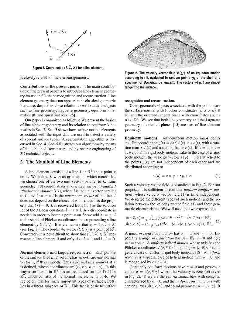
Figure 2. The velocity vector field v(y) of an equiform motionaccording to (1), evaluated in random points yi of the shell of aspecimen of Saxidomus nutalli. The vectors v(yi) are almosttangent to the surface.

recognition and reconstruction.Other geometric objects associated with the point x are

the surface normal with Plucker coordinates (n, x × n) ∈R6 and the oriented tangent plane with coordinates (n, x ·n) ∈ R4. We see that both line geometry and the Laguerregeometry of oriented planes [15] are part of line elementgeometry.

Equiform motions. An equiform motion maps pointsx ∈ R3 according to y(t) = α(t)A(t) ·x+a(t), with a rota-tion matrix A(t) and a scaling factor α(t). If α = const =1, we obtain a rigid body motion. Like in the case of a rigidbody motion, the velocity vectors v(y) = y(t) attached tothe points y(t) are not independent of each other and aredistributed according to

v(y) = c× y + γy + c. (1)

Such a velocity vector field is visualized in Fig. 2. For ourpurposes it is sufficient to consider uniform equiform mo-tions, whose velocity vector field (1) is time independent.We describe the different types of such motions and the re-lation between the velocity vector field (1) and their geo-metric characteristics. We will need the two expressions

z(c, c, γ) = 1γ(c2+γ2) (γc× c− γ2c− (c · c)c) ∈ R3,

A(c, c, γ) = (c, 1c2+γ2 (c2c− (c · c)c + γc× c)) ∈ R6.

(2)

A uniform rigid body motion has α = 1 and γ = 0. Es-pecially a uniform translation has A =E3, c =0 and a(t)= c =const. A uniform helical motion whose axis has thePlucker coordinatesA(c, c, 0) and pitch p = (c ·c)/c2 is thegeneral case of uniform rigid body motions [18]. A uniformrotation is a special case of helical motion with p = 0, andis recognized by c · c = 0.

Genuinely equiform motions have γ 6= 0 and possess acenter z = z(c, c, γ) where the velocity is zero (observedin Fig. 2). There are the central similarities with center z,characterized by c = 0, and the uniform spiral motions withcenter z, axisA(c, c, γ), and spiral parameter p = γ/‖c‖: If

we move z into the origin and the spiral axis into the x3-axisof a Cartesian coordinate system, a spiral motion assumesthe form

y(t) = epωt

[cos ωt − sin ωt 0sin ωt cos ωt 0

0 0 1

]· x, (ω = ‖c‖). (3)

Surfaces generated by spiral motions are used to describethe shape of shells [2, 25]. In Sec. 5 we test to which ex-tent this mathematical model, which is based on exponentialgrowth, agrees with nature.

Linear complexes of line elements. A linear complex ofline elements is defined as the set of line elements whosePlucker coordinates (l, l, λ) satisfy the linear equation

c · l + c · l + γλ = 0 (c, c ∈ R3, γ ∈ R). (4)

We call (c, c, γ) ∈ R7 coordinate vector of the complex. Acurve which undergoes a uniform equiform motion tracesout an equiform kinematic surface. This concept is usedby the following theorem [13] in order to show a relationbetween linear complexes and equiform kinematics:Theorem 1. The surface normal elements of a regular C1

surface in R3 are contained in a linear line element complexwith coordinates (c, c, γ) if and only if the surface is part ofan equiform kinematic surface. In that case the uniformequiform motion has the velocity vector field (1).

The shell of Fig. 2 approximates a kinematic surface verywell, as the velocity vectors v(y) are almost tangent to it.

3. Classification of Surfaces

Consider a sample (li, li, λi) (i = 1, 2, . . . , N , N ≥ 7)of surface normal elements of a surface, taken from pointsin general position. We want to determine if the surface isan equiform kinematic surface, or at least approximately so.

Recognizing kinematic surfaces — the exact case. Wefirst consider data coming from an exact kinematic sur-face and neglect numerical issues. We compute a basisof the space of linear equations of type (4) fulfilled byall (li, li, λi)’s. Assume that this basis is represented bythe coefficient vectors (c1, c1, γ1), . . . (ck, ck, γk) ∈ R7.Note that by Theorem 1, each homogeneous linear equa-tion fulfilled by the given normal element data means auniform equiform motion which transforms the underlyingkinematic surface into itself. The complete classification isgiven below.• k = 4: Only planes are invariant with respect to four inde-pendent uniform motions. It is trivial to find an equation ofthat plane from the given data.• k = 3: Spheres are invariant with respect to a three-parameter family of uniform motions (all of them rotations).The sphere’s center lies on all three rotation axes with Pluc-ker coordinates A(ci, ci, 0) (i = 1, 2, 3).

• k = 2: (2a) A cylinder of revolution is invariant with re-spect to a 2-parameter family of helical motions, spannedby a translation along the helical axis, and by the rotationabout that axis. So for all linear combinations (c, c, γ) =∑2

j=1 µj(cj , cj , γj) except for the one representing thetranslation, A(c, c, γ) is the same, whereas the spiral cen-ter z(c, c, γ) is at infinity (division by zero).

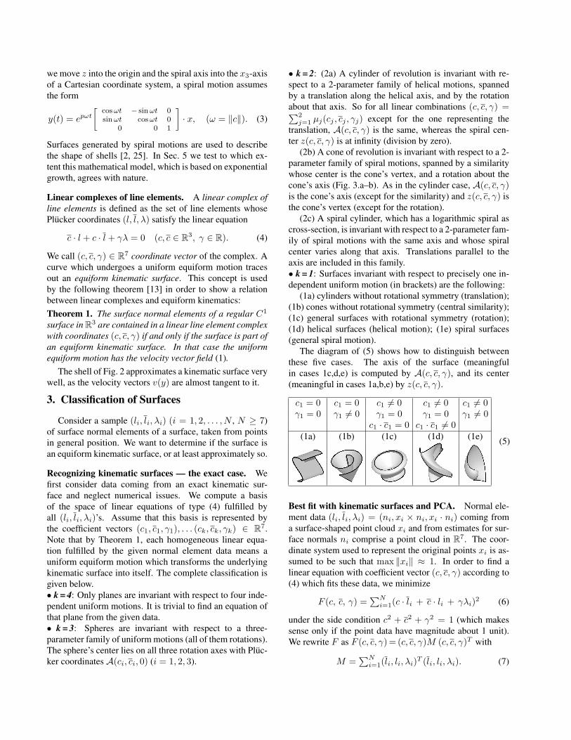
(2b) A cone of revolution is invariant with respect to a 2-parameter family of spiral motions, spanned by a similaritywhose center is the cone’s vertex, and a rotation about thecone’s axis (Fig. 3.a–b). As in the cylinder case, A(c, c, γ)is the cone’s axis (except for the similarity) and z(c, c, γ) isthe cone’s vertex (except for the rotation).

(2c) A spiral cylinder, which has a logarithmic spiral ascross-section, is invariant with respect to a 2-parameter fam-ily of spiral motions with the same axis and whose spiralcenter varies along that axis. Translations parallel to theaxis are included in this family.• k = 1: Surfaces invariant with respect to precisely one in-dependent uniform motion (in brackets) are the following:

(1a) cylinders without rotational symmetry (translation);(1b) cones without rotational symmetry (central similarity);(1c) general surfaces with rotational symmetry (rotation);(1d) helical surfaces (helical motion); (1e) spiral surfaces(general spiral motion).

The diagram of (5) shows how to distinguish betweenthese five cases. The axis of the surface (meaningfulin cases 1c,d,e) is computed by A(c, c, γ), and its center(meaningful in cases 1a,b,e) by z(c, c, γ).

c1 = 0 c1 = 0 c1 6= 0 c1 6= 0 c1 6= 0γ1 = 0 γ1 6= 0 γ1 = 0 γ1 = 0 γ1 6= 0

c1 · c1 = 0 c1 · c1 6= 0(1a) (1b) (1c) (1d) (1e) (5)

Best fit with kinematic surfaces and PCA. Normal ele-ment data (li, li, λi) = (ni, xi × ni, xi · ni) coming froma surface-shaped point cloud xi and from estimates for sur-face normals ni comprise a point cloud in R7. The coor-dinate system used to represent the original points xi is as-sumed to be such that max ‖xi‖ ≈ 1. In order to find alinear equation with coefficient vector (c, c, γ) according to(4) which fits these data, we minimize

F (c, c, γ) =∑N

i=1(c · li + c · li + γλi)2 (6)

under the side condition c2 + c2 + γ2 = 1 (which makessense only if the point data have magnitude about 1 unit).We rewrite F as F (c, c, γ) = (c, c, γ)M (c, c, γ)T with

M =∑N

i=1(li, li, λi)T (li, li, λi). (7)

It is straightforward that an eigenvector (c, c, γ) of M cor-responding to a numerically zero eigenvalue µ leads toan equation of type (4) which is fulfilled by the given(li, li, λi)’s. In that case, F (c, c, γ) = µ. Thus the numberof small eigenvalues of M (one to four) and the correspond-ing eigenvectors determine which type of kinematic surfacethe original point data are approximated with.

Classifying surfaces. When performing the classificationtask on a real data set, the number of decisions to be madeimplies that the setting of thresholds is critical. Numericalexperiments have shown that the strategy described belowworks in a satisfactory way.

(i). Check if the original data are planar or spherical,using well known methods [12, 20]. If they are, go to (v).

(ii). Compute M and its eigenvalues and eigenvec-tors as described above. Sort the eigenvalues µi such that0 ≤ µ1 ≤ µ2 ≤ . . . . The magnitude of eigenvalues is Ntimes length squared, so use νi =

õi/N for comparison

purposes. As spherical and planar surfaces are excluded bynow, the number k of numerically zero eigenvalues of Mcan be 0, 1 or 2. If ν1 is large, the best approximation of thegiven data by a kinematic surface is not very good, and wemay choose not to proceed further (breaking up compositesurfaces is the topic of Sec. 4). Otherwise, two small eigen-values (case k = 2 above) are detected, if ν3/ν2 > ν2/ν1,or if both ν1, ν2 are smaller than a certain threshold.

(iii). In the case k = 2, consider the eigenvectors(ci, ci, γi) (i = 1, 2) and compute the spiral center z(c, c, γ)for a number of linear combinations (c, c, γ) = cos t (c1, c1,γ1) + sin t (c2, c2, γ2) with t = iπ

r , i = 1, . . . , r, r = 20,say (Fig. 3.c). The location of these centers distinguishesbetween cases 2a,b,c . With very noisy data it is helpful tobear in mind that in real life there are no spiral cylinders –if neither 2a nor 2b fits, we might as well move on to (iv)and have the surface type detected again.

(iv). In case of one small eigenvalue, distinguish be-

(a) (b) (c) (d)

Figure 3. (a–b) Velocity vectors on a cone of revolution correspond-ing to eigenvectors (ci, ci, γi) (i = 1, 2) of M via Equ. (1).(c) A sequence of 200 spiral centers and axes computed from linearcombinations of these two eigenvectors. (d) Robustly reconstructedvertex and axis.

tween the cases listed in (5) by choosing appropriate thresh-olds. These are set according to the application we havein mind and the surface types we expect. Genuine spiralsurfaces are rarely observed in machine-made parts, for in-stance. If appropriate, compute axis and center. Finding agenerator curve of the kinematic surface in question fromthe given point data is discussed in Sec. 5.

(v). In all cases we get a kinematic surface Ψ approxi-mating the given point cloud. This least squares fit is maderobust by iteratively downweighting outliers in the defini-tion of M :

M = 1Pσi

∑Ni=1 σi · (li, li, λi)T (li, li, λi), (8)

where σi is a weight penalizing the distance of the data pointxi from Ψ and the distance of the surface normal element(li, li, λi) from the subspace with equation (4).

Inhomogeneous linear equations and offset surfaces.If the inhomogeneous equation c · li + c · li + γλi =k with γ 6= 0 is fulfilled by normal elements (li, li, λi)with ‖li‖ = 1, then the line elements (li, li, λnew

i ) withλi − λnew

i = k/γ fulfill the homogeneous equation (4).The change λi → λnew

i means moving the point xi toxi − k

γ li. Fortunately the new elements are normal ele-ments of a surface again, namely of an offset at distancek/γ of the original data. By minimizing F (c, c, γ, k) =∑N

i=1(c · li + c · li + γλi − k)2 we can find an offset of akinematic surface which approximates the given data, pro-vided γ turns out to be nonzero.

4. Segmentation

The bottom up approach to segmentation, where localshape detectors classify small surface patches, which aresubsequently fitted together is e.g. used by N. Gelfand andL. Guibas in [3]. They employ Euclidean kinematics andline geometry in a way similar to our use of equiform kine-matics and line element geometry.

We use a top-down multi-pass algorithm which first de-tects planes and spheres, then the cases 2a+b of Sec. 3, andat last the remaining cases. The description of the first pass,which uses RANSAC in the well known way together withline element geometry serves also as an introduction into thenext one, where line element geometry is more prominent.

Detecting planar and spherical surfaces. The proceduredescribed by this paragraph is standard. For a random sam-ple of centers chosen from the original data set (denoted byC), we determine neighbourhoods Ni. Size and number ofthe Ni’s are chosen in relation to the complexity of the dataset: A substantial part of at least some Ni’s should be cov-ered by a single surface detected by the procedure. We usethe RANSAC principle [4] as follows: R times we choosefour random points in Ni, fit a sphere Ψij to them, and find

(a) (b)

Figure 4. (a) Support Sij of sphere (dark) computed from point dataonly. (b) Sij trimmed using line element data.

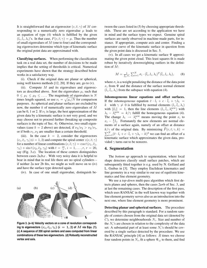
the set Sij of points x ∈ C which fulfill dist(x,Ψij) < δ.For the choice of R we follow [4], p. 104 and let R = 25;for the choice of δ we take the noise level of C into ac-count. If Ψij’s radius is very large, we fit a plane instead ofa sphere and recompute Sij . Sij is the support of the sur-face Ψij (Fig. 4.a). Ψij’s with large support are investigatedmore closely (see next paragraph).

Trimming supports. Some vertices of C close to thesphere/plane Ψij are not contained in the spherical/planarface of the given surface which we want to detect (Fig. 4.a).Their normal elements (lr, lr, λr) do not satisfy (4), where(c, c, γ) is any linear complex belonging to the kinematicsurface Ψij according to Theorem 1 and the discussionin Sec. 3. Thus we choose exact normal line elementsfrom Ψij , compute M and the eigenvectors (ci, ci, γi) fori = 1, . . . , k as in Sec. 3 (k = 3 for a sphere and k = 4 fora plane). A data point is kept in the support Sij only if itsnormal element satisfies∑k

i=1(ci · lr + ci · lr + γiλr)2 < δ2. (9)

See Fig. 4.b for such a trimmed support. We finally markthe support as a surface detected and iterate, until supportsof spheres and planes detected become too small. This con-cludes pass 1 of the algorithm.

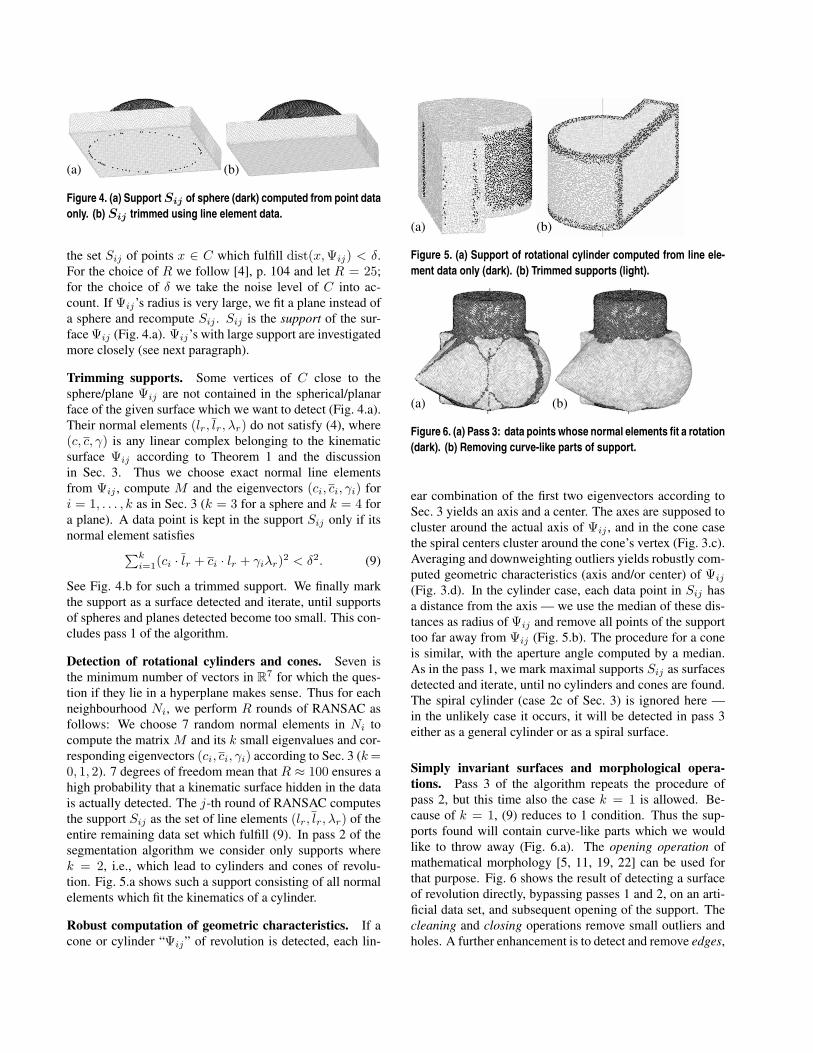
Detection of rotational cylinders and cones. Seven isthe minimum number of vectors in R7 for which the ques-tion if they lie in a hyperplane makes sense. Thus for eachneighbourhood Ni, we perform R rounds of RANSAC asfollows: We choose 7 random normal elements in Ni tocompute the matrix M and its k small eigenvalues and cor-responding eigenvectors (ci, ci, γi) according to Sec. 3 (k =0, 1, 2). 7 degrees of freedom mean that R ≈ 100 ensures ahigh probability that a kinematic surface hidden in the datais actually detected. The j-th round of RANSAC computesthe support Sij as the set of line elements (lr, lr, λr) of theentire remaining data set which fulfill (9). In pass 2 of thesegmentation algorithm we consider only supports wherek = 2, i.e., which lead to cylinders and cones of revolu-tion. Fig. 5.a shows such a support consisting of all normalelements which fit the kinematics of a cylinder.

Robust computation of geometric characteristics. If acone or cylinder “Ψij” of revolution is detected, each lin-

(a) (b)

Figure 5. (a) Support of rotational cylinder computed from line ele-ment data only (dark). (b) Trimmed supports (light).

(a) (b)

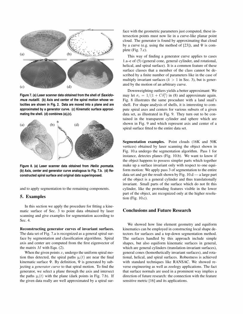
Figure 6. (a) Pass 3: data points whose normal elements fit a rotation(dark). (b) Removing curve-like parts of support.

ear combination of the first two eigenvectors according toSec. 3 yields an axis and a center. The axes are supposed tocluster around the actual axis of Ψij , and in the cone casethe spiral centers cluster around the cone’s vertex (Fig. 3.c).Averaging and downweighting outliers yields robustly com-puted geometric characteristics (axis and/or center) of Ψij

(Fig. 3.d). In the cylinder case, each data point in Sij hasa distance from the axis — we use the median of these dis-tances as radius of Ψij and remove all points of the supporttoo far away from Ψij (Fig. 5.b). The procedure for a coneis similar, with the aperture angle computed by a median.As in the pass 1, we mark maximal supports Sij as surfacesdetected and iterate, until no cylinders and cones are found.The spiral cylinder (case 2c of Sec. 3) is ignored here —in the unlikely case it occurs, it will be detected in pass 3either as a general cylinder or as a spiral surface.

Simply invariant surfaces and morphological opera-tions. Pass 3 of the algorithm repeats the procedure ofpass 2, but this time also the case k = 1 is allowed. Be-cause of k = 1, (9) reduces to 1 condition. Thus the sup-ports found will contain curve-like parts which we wouldlike to throw away (Fig. 6.a). The opening operation ofmathematical morphology [5, 11, 19, 22] can be used forthat purpose. Fig. 6 shows the result of detecting a surfaceof revolution directly, bypassing passes 1 and 2, on an arti-ficial data set, and subsequent opening of the support. Thecleaning and closing operations remove small outliers andholes. A further enhancement is to detect and remove edges,

(a) (b)

(c) (d)

Figure 7. (a) Laser scanner data obtained from the shell of Saxido-mus nutalli. (b) Axis and center of the spiral motion whose ve-locities are shown in Fig. 2. Data are moved into a plane and areapproximated by a generator curve. (c) Kinematic surface approxi-mating the shell. (d) combines (a),(c).

(a) (b) (d)

Figure 8. (a) Laser scanner data obtained from Helix pomata.(b) Axis, center and generator curve analogous to Fig. 7.b. (d) Re-constructed spiral surface and original data superimposed.

and to apply segmentation to the remaining components.

5. Examples

In this section we apply the procedure for fitting a kine-matic surface of Sec. 3 to point data obtained by laserscanning and give examples for segmentation according toSec. 4.

Reconstructing generator curves of invariant surfaces.The data set of Fig. 7.a is recognized as a general spiral sur-face by segmentation and classification algorithms. Spiralaxis and center are computed from the first eigenvector ofthe matrix M with Equ. (2).

When the given points xi undergo the uniform spiral mo-tion thus detected, the spiral paths yi(t) are near the finalkinematic surface Ψ. By definition, Ψ is generated by sub-jecting a generator curve to that spiral motion. To find thegenerator, we select a plane through the axis and intersectthe paths yi(t) with the plane (dark points in Fig. 7.b). Ifthe given data really are well approximated by a spiral sur-

face with the geometric parameters just computed, these in-tersection points must now lie in a curve-like planar pointcloud. The generator is found by approximating that cloudby a curve (e.g. using the method of [23]), and Ψ is com-plete (Fig. 7.c).

This way of finding a generator curve applies to cases1.a–e of (5) (general cone, general cylinder, and rotational,helical, and spiral surface). It is a common feature of thesesurface classes that a member of the class cannot be de-scribed by a finite number of parameters like in the case ofmultiply invariant surfaces (k > 1 in Sec. 3), but is gener-ated by the motion of an arbitrary curve.

Downweighting outliers yields a better approximant: Wemay let σi = 1/(1 + Cδ2

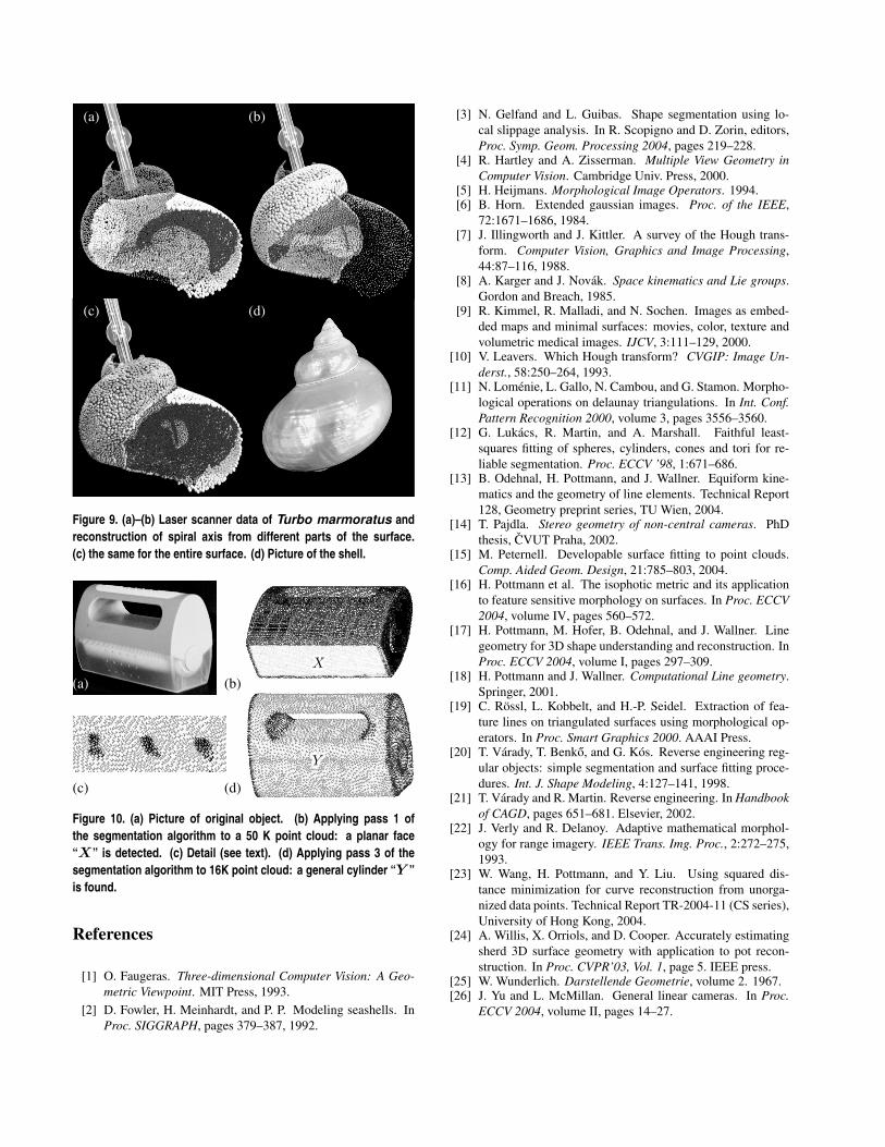
i ) in (8) and approximate again.Fig. 8 illustrates the same procudure with a land snail’sshell. For shape analysis of shells, it is interesting to com-pute spiral axes and centers for various subsets of a givendata set, as illustrated in Fig. 9. They turn out to be con-tained in the transparent cylinder and sphere which areshown in Fig. 9 and which represent axis and center of aspiral surface fitted to the entire data set.

Segmentation examples. Point clouds (16K and 50Kvertices) obtained by laser scanning the object shown inFig. 10.a undergo the segmentation algorithm. Pass 1 forinstance, detectes planes (Fig. 10.b). We want to know ifthe object happens to possess simpler parts which togethermake up a surface invariant only with respect to one equi-form motion: We apply pass 3 of segmentation to the entiredata set and get the result shown by Fig. 10.d — a large partof the object is a general cylinder and thus translationallyinvariant. Small parts of the surface which do not fit thiscylinder, like the protruding features visible in the lowerpart of the object, are recognized only at the higher resolu-tion (Fig. 10.c).

Conclusions and Future Research

We showed how line element geometry and equiformkinematics can be employed in constructing local shape de-tectors for surfaces and a top-down segmentation method.The surfaces handled by this approach include simpleshapes, but also equiform kinematic surfaces in general,which are general cylinders (translation-invariant surfaces),general cones (homothetically invariant surfaces), and rota-tional, helical, and spiral surfaces. Robustness is achievedwith standard techniques like RANSAC. We showed re-verse engineering as well as zoology applications. The factthat surface normals are used in a prominent way implies adirection of future research: the connection with the featuresensitive metric [16] and its applications.

(a) (b)

(c) (d)

Figure 9. (a)–(b) Laser scanner data of Turbo marmoratus andreconstruction of spiral axis from different parts of the surface.(c) the same for the entire surface. (d) Picture of the shell.

XXXXXXXXXXXXXXXXX

(a) (b)

YYYYYYYYYYYYYYYYY

(c) (d)

Figure 10. (a) Picture of original object. (b) Applying pass 1 ofthe segmentation algorithm to a 50 K point cloud: a planar face“X” is detected. (c) Detail (see text). (d) Applying pass 3 of thesegmentation algorithm to 16K point cloud: a general cylinder “Y ”is found.

References

[1] O. Faugeras. Three-dimensional Computer Vision: A Geo-metric Viewpoint. MIT Press, 1993.

[2] D. Fowler, H. Meinhardt, and P. P. Modeling seashells. InProc. SIGGRAPH, pages 379–387, 1992.

[3] N. Gelfand and L. Guibas. Shape segmentation using lo-cal slippage analysis. In R. Scopigno and D. Zorin, editors,Proc. Symp. Geom. Processing 2004, pages 219–228.

[4] R. Hartley and A. Zisserman. Multiple View Geometry inComputer Vision. Cambridge Univ. Press, 2000.

[5] H. Heijmans. Morphological Image Operators. 1994.[6] B. Horn. Extended gaussian images. Proc. of the IEEE,

72:1671–1686, 1984.[7] J. Illingworth and J. Kittler. A survey of the Hough trans-

form. Computer Vision, Graphics and Image Processing,44:87–116, 1988.

[8] A. Karger and J. Novak. Space kinematics and Lie groups.Gordon and Breach, 1985.

[9] R. Kimmel, R. Malladi, and N. Sochen. Images as embed-ded maps and minimal surfaces: movies, color, texture andvolumetric medical images. IJCV, 3:111–129, 2000.

[10] V. Leavers. Which Hough transform? CVGIP: Image Un-derst., 58:250–264, 1993.

[11] N. Lomenie, L. Gallo, N. Cambou, and G. Stamon. Morpho-logical operations on delaunay triangulations. In Int. Conf.Pattern Recognition 2000, volume 3, pages 3556–3560.

[12] G. Lukacs, R. Martin, and A. Marshall. Faithful least-squares fitting of spheres, cylinders, cones and tori for re-liable segmentation. Proc. ECCV ’98, 1:671–686.

[13] B. Odehnal, H. Pottmann, and J. Wallner. Equiform kine-matics and the geometry of line elements. Technical Report128, Geometry preprint series, TU Wien, 2004.

[14] T. Pajdla. Stereo geometry of non-central cameras. PhDthesis, CVUT Praha, 2002.

[15] M. Peternell. Developable surface fitting to point clouds.Comp. Aided Geom. Design, 21:785–803, 2004.

[16] H. Pottmann et al. The isophotic metric and its applicationto feature sensitive morphology on surfaces. In Proc. ECCV2004, volume IV, pages 560–572.

[17] H. Pottmann, M. Hofer, B. Odehnal, and J. Wallner. Linegeometry for 3D shape understanding and reconstruction. InProc. ECCV 2004, volume I, pages 297–309.

[18] H. Pottmann and J. Wallner. Computational Line geometry.Springer, 2001.

[19] C. Rossl, L. Kobbelt, and H.-P. Seidel. Extraction of fea-ture lines on triangulated surfaces using morphological op-erators. In Proc. Smart Graphics 2000. AAAI Press.

[20] T. Varady, T. Benko, and G. Kos. Reverse engineering reg-ular objects: simple segmentation and surface fitting proce-dures. Int. J. Shape Modeling, 4:127–141, 1998.

[21] T. Varady and R. Martin. Reverse engineering. In Handbookof CAGD, pages 651–681. Elsevier, 2002.

[22] J. Verly and R. Delanoy. Adaptive mathematical morphol-ogy for range imagery. IEEE Trans. Img. Proc., 2:272–275,1993.

[23] W. Wang, H. Pottmann, and Y. Liu. Using squared dis-tance minimization for curve reconstruction from unorga-nized data points. Technical Report TR-2004-11 (CS series),University of Hong Kong, 2004.

[24] A. Willis, X. Orriols, and D. Cooper. Accurately estimatingsherd 3D surface geometry with application to pot recon-struction. In Proc. CVPR’03, Vol. 1, page 5. IEEE press.

[25] W. Wunderlich. Darstellende Geometrie, volume 2. 1967.[26] J. Yu and L. McMillan. General linear cameras. In Proc.

ECCV 2004, volume II, pages 14–27.