Byrd 1

3D Motion-Tracking PET Experimental Prototype Final

Report

Brook Byrd

April 28th, 2017

Mentors: Drew Weisenberger, Brian Kross, John McKisson, Jack McKisson, Carl Zorn, Wenze Xi, and Seung Joon Lee

CNU Advisor: David Heddle

Byrd 2

1. Abstract In highly controlled settings, PET brain imaging is currently performed to detect a wide

array of diseases and to assess brain functionality. However, most brain imaging PET systems require the patient to be prone or supine and highly restrained. If the patient was able to be imaged in a natural environment instead of a constricted one, it would open up new frontiers for studying brain physiology and PET tracer biokinetics during normal and specialized activities. Researchers within the Jefferson Lab Detector Group and collaborators have proposed the RoomPET, a clinical system in which a person could be normally functioning while a hidden PET system images the brain with resolution up to clinical standards. Such a system presents a large number of challenges. As a proof of principle, a 3D Motion-Tracking PET prototype was created with necessary gantry mechanics, tracking abilities, and control systems to enable horizontal transitions which keep a target within the PET field of view. Utilizing fiducial markers, a vision system provides positional information for a list-mode image reconstruction. In response to target motion, the motor control system can perform horizontal transitions which allows the target to remain within the PET field of view.

This system allowed the performance of the vision system to be examined in depth. A number of tests were conducted on the vision system’s accuracy and precision in reporting positional values under a variety of gantry movement behaviors. Tests were conducted under stationary and constant velocity conditions.

All positional errors were found to be under 300 micrometers which is well within clinical standards. With internal averaging taking place in the tracking software, raw positional output can be acquired at the rate of 60 frames per second without need for additional averaging. While the average appears to shift over a prolonged data acquisition period, instantaneous positional readings acquired within 10 seconds have a standard deviation of less than 20 micrometers.

The vision system is able to report the position of the detector and the target with the precision of micrometers. Correlations were found between positional error and target velocity. Repeated trials showed that velocity measurements can be recorded with less than a 1% error between the measured velocity and the user-commanded velocity. In conclusion, the vision system's performance results provide strong support that positional accuracy is achievable for successful image reconstruction in both static conditions and under motion.

Byrd 3

2. Acknowledgement I would like to thank the Jefferson Lab Detector and Imaging group who provided the

facilities, insight, and expertise which greatly assisted with the progression of this project. I also would like to thank Mark Smith from the University of Maryland Baltimore for lending equipment and materials. Finally, I would like to thank Dr. David Heddle for his gracious funding and mentorship throughout this project.

3. Introduction The ability to examine assess brain function of subjects within a natural environment

without immobilizing confinements is the principle motivation driving the development of the RoomPET. Understanding brain functionality under a wide array of activities could provide a breakthrough in the realm of neurology. While covering the entire surface area of the room with PET detectors for 100% geometric sensitivity is desirable, it is not practically feasible given the prohibitive cost. Therefore, the concept behind the RoomPET is to adjust the position of a moving PET detectors outside of the room to effectively follow the subject’s head.

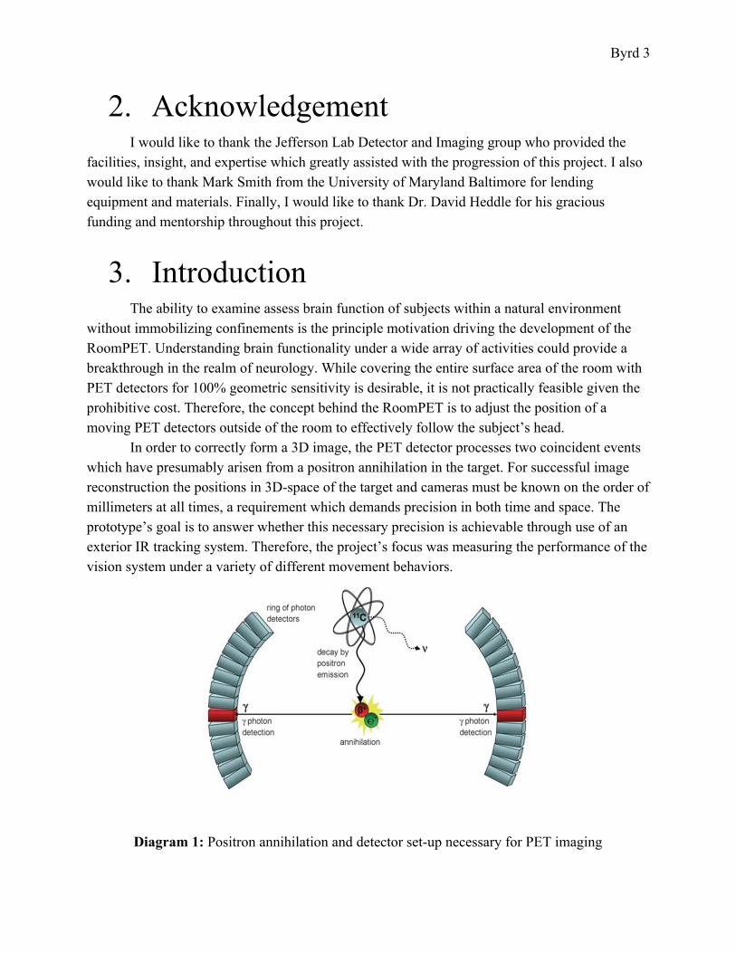
In order to correctly form a 3D image, the PET detector processes two coincident events which have presumably arisen from a positron annihilation in the target. For successful image reconstruction the positions in 3D-space of the target and cameras must be known on the order of millimeters at all times, a requirement which demands precision in both time and space. The prototype’s goal is to answer whether this necessary precision is achievable through use of an exterior IR tracking system. Therefore, the project’s focus was measuring the performance of the vision system under a variety of different movement behaviors.

Diagram 1: Positron annihilation and detector set-up necessary for PET imaging

Byrd 4

The two main hypotheses were: positional error will be dependent on geometric setup, and positional error will increase linearly with velocity. To test these and other performance metrics, a series of experimental runs took place as time-stamped positional data was streamed into a text file for further analysis.

4. Theory

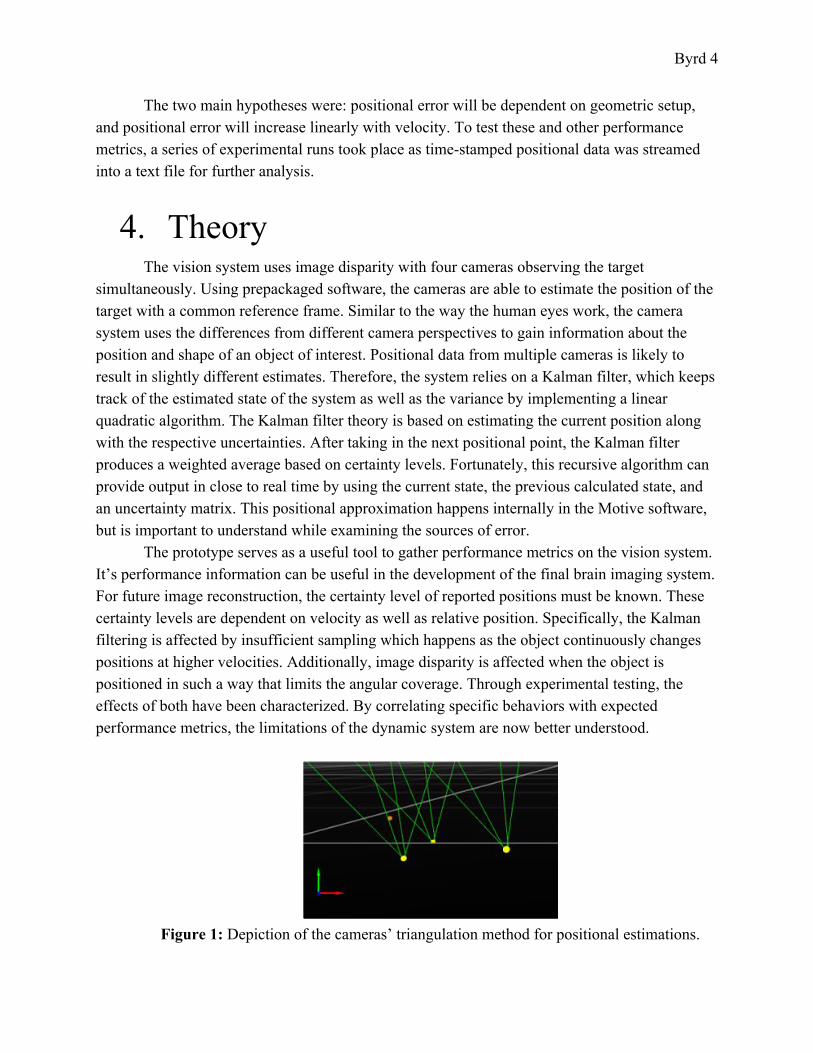
The vision system uses image disparity with four cameras observing the target simultaneously. Using prepackaged software, the cameras are able to estimate the position of the target with a common reference frame. Similar to the way the human eyes work, the camera system uses the differences from different camera perspectives to gain information about the position and shape of an object of interest. Positional data from multiple cameras is likely to result in slightly different estimates. Therefore, the system relies on a Kalman filter, which keeps track of the estimated state of the system as well as the variance by implementing a linear quadratic algorithm. The Kalman filter theory is based on estimating the current position along with the respective uncertainties. After taking in the next positional point, the Kalman filter produces a weighted average based on certainty levels. Fortunately, this recursive algorithm can provide output in close to real time by using the current state, the previous calculated state, and an uncertainty matrix. This positional approximation happens internally in the Motive software, but is important to understand while examining the sources of error.

The prototype serves as a useful tool to gather performance metrics on the vision system. It’s performance information can be useful in the development of the final brain imaging system. For future image reconstruction, the certainty level of reported positions must be known. These certainty levels are dependent on velocity as well as relative position. Specifically, the Kalman filtering is affected by insufficient sampling which happens as the object continuously changes positions at higher velocities. Additionally, image disparity is affected when the object is positioned in such a way that limits the angular coverage. Through experimental testing, the effects of both have been characterized. By correlating specific behaviors with expected performance metrics, the limitations of the dynamic system are now better understood.

Figure 1: Depiction of the cameras’ triangulation method for positional estimations.

Byrd 5

While analyzing the performance metrics, it was valuable to separate and understand the

various sources of the error. A number of different methods was used to categorize each kind of error. As a result, all five kinds of error were successfully identified and characterized through experimentation. The quantification of these errors revealed a number of limitations that will need to be taken into consideration during image reconstruction.

The errors further investigated include: random error, offset error, scale error, mechanical error, and errors associated with specific movement behaviors. Randomly distributed errors are called noise. Random noise was inspected by holding the stage motionless as positional data was continuously collected over a long span of time. While this noise can not be eliminated, it is useful to understand the pre-existing background noise in the system. Spatial-dependent variances in performance can be attributed to scale error within the system. Scale error was inspected by measuring the positional error at uniform increments along the track and comparing performance metrics. Offset error is a function of the measurement method, which in this case will be the vision system. In this system, offset error was examined by comparing the commanded transitions and velocities with the experimentally measured transitions and velocities. Additionally, mechanical error can be identified by periodic inconsistencies that occur consistently within a system. Lastly, errors associated with movement were inspected by moving the stage at constant velocity at three different speeds.

Interestingly, the most significant error surfaced from a ‘settling’ effect found in tracking a stationary point over a prolonged amount of time. As the position shifted by 300 µm over the course of an hour in multiple experimental set-ups, clearly the absolute position in the vision system’s frame of reference shifted over time. This was the most significant error, and points to the important conclusions that the vision system’s reported absolute positions are not reliable. To provide a proper, non-stationary absolute point of reference, an additional fiducial marker will be needed in the final system. With an additional geographic reference, the vision system’s shifting can be accounted for and recorrected. In conclusion, relationships between velocity, space, sample-time, and tracking performance were all able to be identified through this series of experiments.

Byrd 6

5. Methods Before measurement could be made, the vision system was calibrated through a

prepackaged software. After installing the Optitrack interface software on the PC, the cameras automatically named themselves and started recording images which could be seen on the Optitrack interface. With this connection established, the frame rate per second, exposure, threshold, and LED illumination levels were separately adjusted until a clear image was displayed with minimal background infrared light. This was only the beginning of a regimented calibration routine that needed to be followed precisely as stated in the Optitrack user manual.

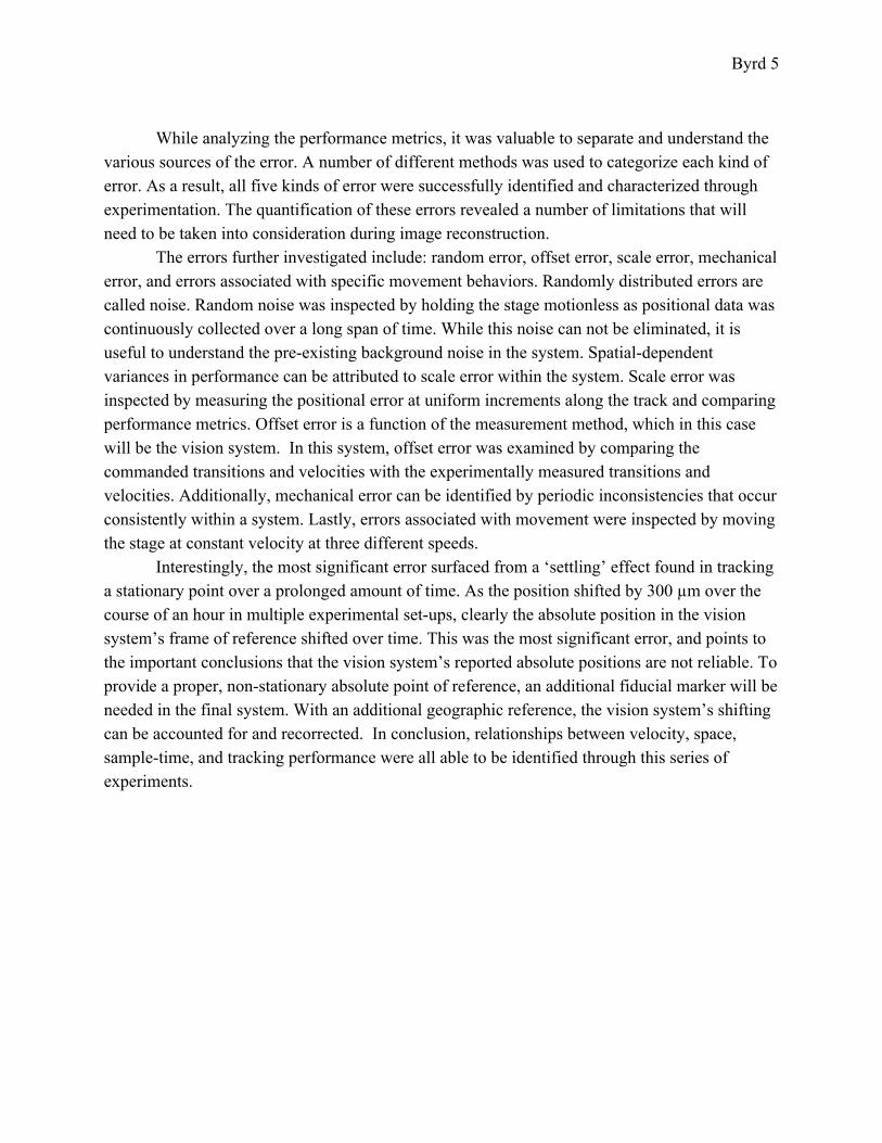
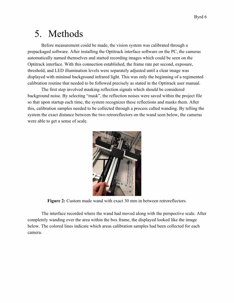
The first step involved masking reflection signals which should be considered background noise. By selecting “mask”, the reflection noises were saved within the project file so that upon startup each time, the system recognizes these reflections and masks them. After this, calibration samples needed to be collected through a process called wanding. By telling the system the exact distance between the two retroreflectors on the wand seen below, the cameras were able to get a sense of scale.

Figure 2: Custom made wand with exact 30 mm in between retroreflectors.

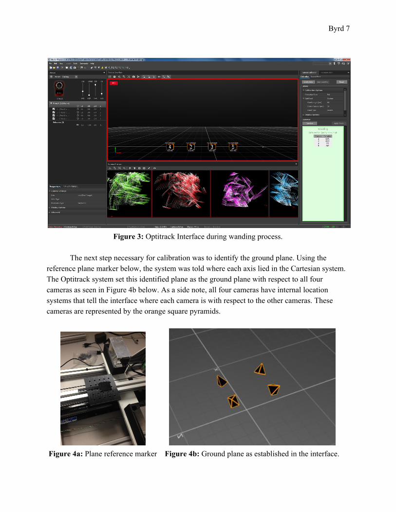
The interface recorded where the wand had moved along with the perspective scale. After

completely wanding over the area within the box frame, the displayed looked like the image below. The colored lines indicate which areas calibration samples had been collected for each camera.

Byrd 7

Figure 3: Optitrack Interface during wanding process.

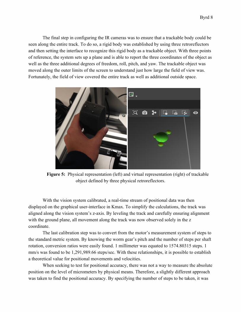
The next step necessary for calibration was to identify the ground plane. Using the

reference plane marker below, the system was told where each axis lied in the Cartesian system. The Optitrack system set this identified plane as the ground plane with respect to all four cameras as seen in Figure 4b below. As a side note, all four cameras have internal location systems that tell the interface where each camera is with respect to the other cameras. These cameras are represented by the orange square pyramids.

Figure 4a: Plane reference marker Figure 4b: Ground plane as established in the interface.

Byrd 8

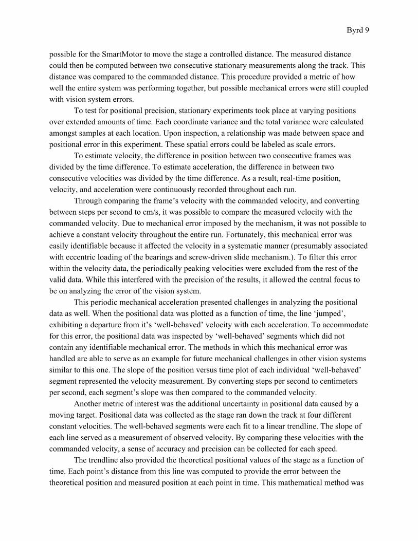
The final step in configuring the IR cameras was to ensure that a trackable body could be

seen along the entire track. To do so, a rigid body was established by using three retroreflectors and then setting the interface to recognize this rigid body as a trackable object. With three points of reference, the system sets up a plane and is able to report the three coordinates of the object as well as the three additional degrees of freedom, roll, pitch, and yaw. The trackable object was moved along the outer limits of the screen to understand just how large the field of view was. Fortunately, the field of view covered the entire track as well as additional outside space.

Figure 5: Physical representation (left) and virtual representation (right) of trackable

object defined by three physical retroreflectors.

With the vision system calibrated, a real-time stream of positional data was then displayed on the graphical user-interface in Kmax. To simplify the calculations, the track was aligned along the vision system’s z-axis. By leveling the track and carefully ensuring alignment with the ground plane, all movement along the track was now observed solely in the z coordinate.

The last calibration step was to convert from the motor’s measurement system of steps to the standard metric system. By knowing the worm gear’s pitch and the number of steps per shaft rotation, conversion ratios were easily found. 1 millimeter was equated to 1574.80315 steps. 1 mm/s was found to be 1,291,989.66 steps/sec. With these relationships, it is possible to establish a theoretical value for positional movements and velocities.

When seeking to test for positional accuracy, there was not a way to measure the absolute position on the level of micrometers by physical means. Therefore, a slightly different approach was taken to find the positional accuracy. By specifying the number of steps to be taken, it was

Byrd 9

possible for the SmartMotor to move the stage a controlled distance. The measured distance could then be computed between two consecutive stationary measurements along the track. This distance was compared to the commanded distance. This procedure provided a metric of how well the entire system was performing together, but possible mechanical errors were still coupled with vision system errors.

To test for positional precision, stationary experiments took place at varying positions over extended amounts of time. Each coordinate variance and the total variance were calculated amongst samples at each location. Upon inspection, a relationship was made between space and positional error in this experiment. These spatial errors could be labeled as scale errors.

To estimate velocity, the difference in position between two consecutive frames was divided by the time difference. To estimate acceleration, the difference in between two consecutive velocities was divided by the time difference. As a result, real-time position, velocity, and acceleration were continuously recorded throughout each run.

Through comparing the frame’s velocity with the commanded velocity, and converting between steps per second to cm/s, it was possible to compare the measured velocity with the commanded velocity. Due to mechanical error imposed by the mechanism, it was not possible to achieve a constant velocity throughout the entire run. Fortunately, this mechanical error was easily identifiable because it affected the velocity in a systematic manner (presumably associated with eccentric loading of the bearings and screw-driven slide mechanism.). To filter this error within the velocity data, the periodically peaking velocities were excluded from the rest of the valid data. While this interfered with the precision of the results, it allowed the central focus to be on analyzing the error of the vision system.

This periodic mechanical acceleration presented challenges in analyzing the positional data as well. When the positional data was plotted as a function of time, the line ‘jumped’, exhibiting a departure from it’s ‘well-behaved’ velocity with each acceleration. To accommodate for this error, the positional data was inspected by ‘well-behaved’ segments which did not contain any identifiable mechanical error. The methods in which this mechanical error was handled are able to serve as an example for future mechanical challenges in other vision systems similar to this one. The slope of the position versus time plot of each individual ‘well-behaved’ segment represented the velocity measurement. By converting steps per second to centimeters per second, each segment’s slope was then compared to the commanded velocity.

Another metric of interest was the additional uncertainty in positional data caused by a moving target. Positional data was collected as the stage ran down the track at four different constant velocities. The well-behaved segments were each fit to a linear trendline. The slope of each line served as a measurement of observed velocity. By comparing these velocities with the commanded velocity, a sense of accuracy and precision can be collected for each speed.

The trendline also provided the theoretical positional values of the stage as a function of time. Each point’s distance from this line was computed to provide the error between the theoretical position and measured position at each point in time. This mathematical method was

Byrd 10

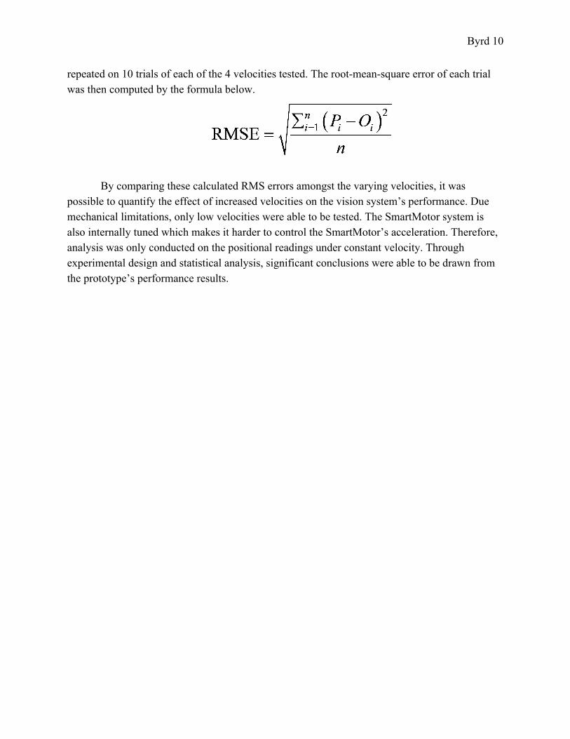
repeated on 10 trials of each of the 4 velocities tested. The root-mean-square error of each trial was then computed by the formula below.

By comparing these calculated RMS errors amongst the varying velocities, it was

possible to quantify the effect of increased velocities on the vision system’s performance. Due mechanical limitations, only low velocities were able to be tested. The SmartMotor system is also internally tuned which makes it harder to control the SmartMotor’s acceleration. Therefore, analysis was only conducted on the positional readings under constant velocity. Through experimental design and statistical analysis, significant conclusions were able to be drawn from the prototype’s performance results.

Byrd 11

6. Data There was no way to measure the absolute location of the stage on the level of

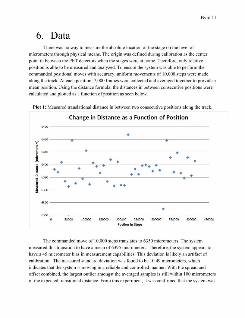
micrometers through physical means. The origin was defined during calibration as the center point in between the PET detectors when the stages were at home. Therefore, only relative position is able to be measured and analyzed. To ensure the system was able to perform the commanded positional moves with accuracy, uniform movements of 10,000 steps were made along the track. At each position, 7,000 frames were collected and averaged together to provide a mean position. Using the distance formula, the distances in between consecutive positions were calculated and plotted as a function of position as seen below.

Plot 1: Measured translational distance in between two consecutive positions along the track.

The commanded move of 10,000 steps translates to 6350 micrometers. The system measured this transition to have a mean of 6395 micrometers. Therefore, the system appears to have a 45 micrometer bias in measurement capabilities. This deviation is likely an artifact of calibration. The measured standard deviation was found to be 10.49 micrometers, which indicates that the system is moving in a reliable and controlled manner. With the spread and offset combined, the largest outlier amongst the averaged samples is still within 100 micrometers of the expected transitional distance. From this experiment, it was confirmed that the system was

Byrd 12

operating in a dependable manner and future statistical analysis on vision system performance could proceed

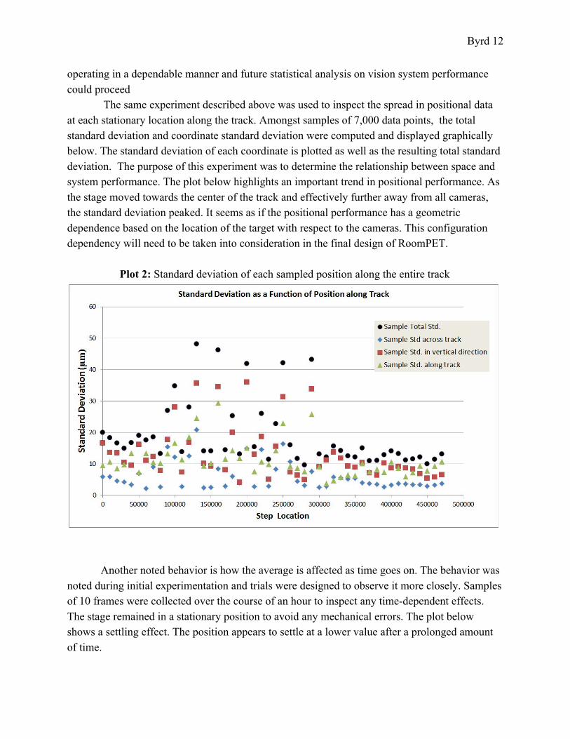
The same experiment described above was used to inspect the spread in positional data at each stationary location along the track. Amongst samples of 7,000 data points, the total standard deviation and coordinate standard deviation were computed and displayed graphically below. The standard deviation of each coordinate is plotted as well as the resulting total standard deviation. The purpose of this experiment was to determine the relationship between space and system performance. The plot below highlights an important trend in positional performance. As the stage moved towards the center of the track and effectively further away from all cameras, the standard deviation peaked. It seems as if the positional performance has a geometric dependence based on the location of the target with respect to the cameras. This configuration dependency will need to be taken into consideration in the final design of RoomPET.

Plot 2: Standard deviation of each sampled position along the entire track

Another noted behavior is how the average is affected as time goes on. The behavior was

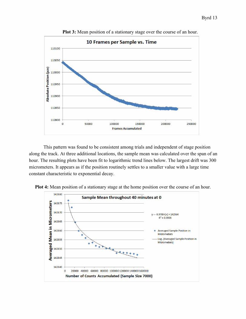
noted during initial experimentation and trials were designed to observe it more closely. Samples of 10 frames were collected over the course of an hour to inspect any time-dependent effects. The stage remained in a stationary position to avoid any mechanical errors. The plot below shows a settling effect. The position appears to settle at a lower value after a prolonged amount of time.

Byrd 13

Plot 3: Mean position of a stationary stage over the course of an hour.

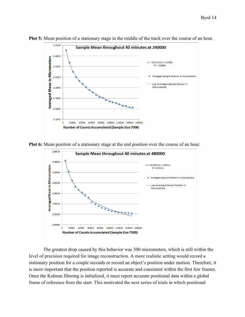
This pattern was found to be consistent among trials and independent of stage position

along the track. At three additional locations, the sample mean was calculated over the span of an hour. The resulting plots have been fit to logarithmic trend lines below. The largest drift was 300 micrometers. It appears as if the position routinely settles to a smaller value with a large time constant characteristic to exponential decay.

Plot 4: Mean position of a stationary stage at the home position over the course of an hour.

Byrd 14

Plot 5: Mean position of a stationary stage in the middle of the track over the course of an hour.

Plot 6: Mean position of a stationary stage at the end position over the course of an hour.

The greatest drop caused by this behavior was 300 micrometers, which is still within the

level of precision required for image reconstruction. A more realistic setting would record a stationary position for a couple seconds or record an object’s position under motion. Therefore, it is more important that the position reported is accurate and consistent within the first few frames. Once the Kalman filtering is initialized, it must report accurate positional data within a global frame of reference from the start. This motivated the next series of trials in which positional

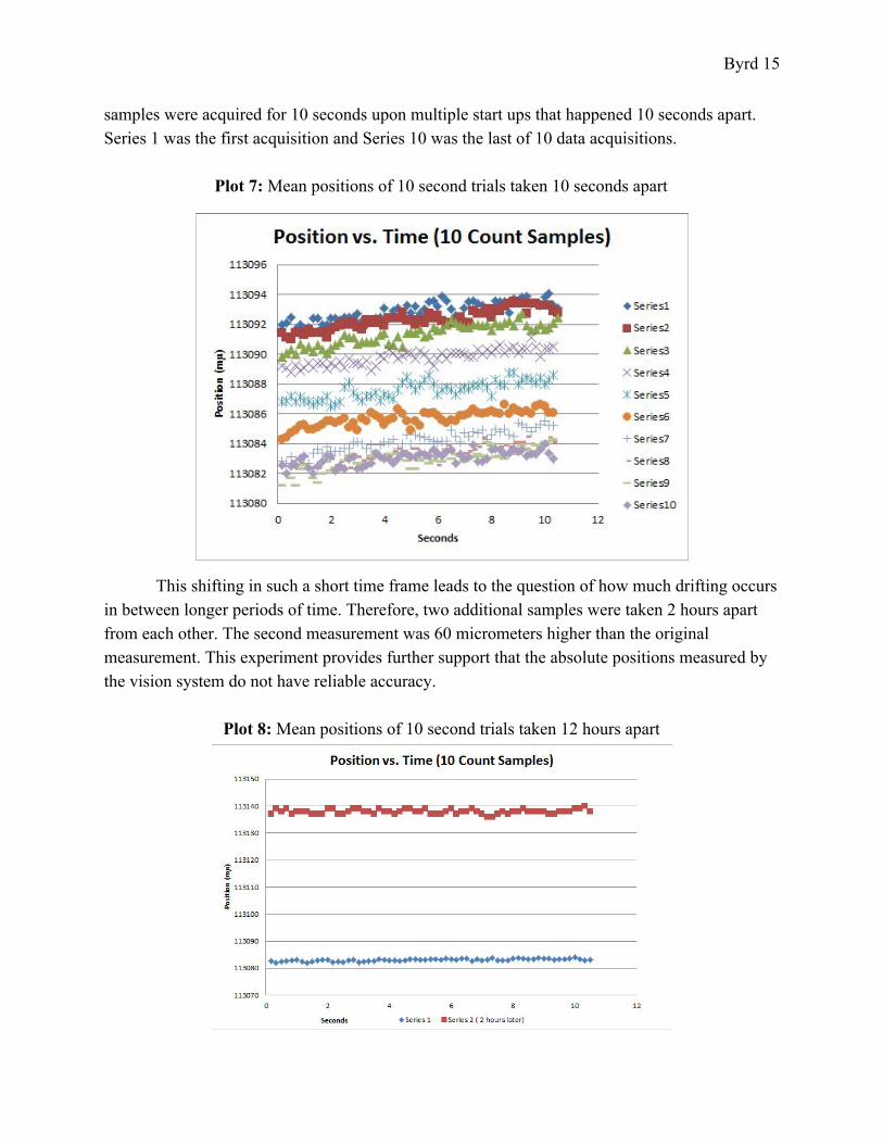
Byrd 15

samples were acquired for 10 seconds upon multiple start ups that happened 10 seconds apart. Series 1 was the first acquisition and Series 10 was the last of 10 data acquisitions.

Plot 7: Mean positions of 10 second trials taken 10 seconds apart

This shifting in such a short time frame leads to the question of how much drifting occurs in between longer periods of time. Therefore, two additional samples were taken 2 hours apart from each other. The second measurement was 60 micrometers higher than the original measurement. This experiment provides further support that the absolute positions measured by the vision system do not have reliable accuracy.

Plot 8: Mean positions of 10 second trials taken 12 hours apart

Byrd 16

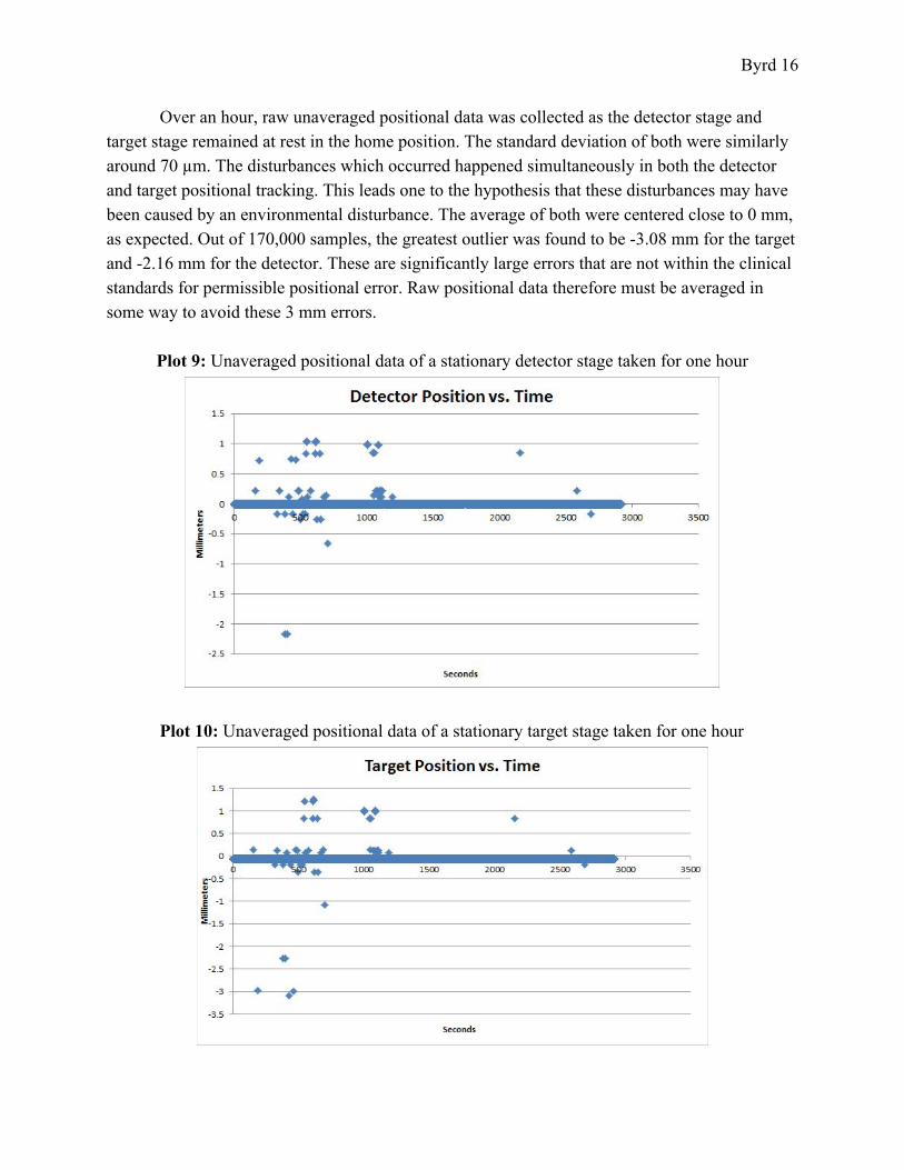
Over an hour, raw unaveraged positional data was collected as the detector stage and target stage remained at rest in the home position. The standard deviation of both were similarly around 70 µm. The disturbances which occurred happened simultaneously in both the detector and target positional tracking. This leads one to the hypothesis that these disturbances may have been caused by an environmental disturbance. The average of both were centered close to 0 mm, as expected. Out of 170,000 samples, the greatest outlier was found to be -3.08 mm for the target and -2.16 mm for the detector. These are significantly large errors that are not within the clinical standards for permissible positional error. Raw positional data therefore must be averaged in some way to avoid these 3 mm errors.

Plot 9: Unaveraged positional data of a stationary detector stage taken for one hour

Plot 10: Unaveraged positional data of a stationary target stage taken for one hour

Byrd 17

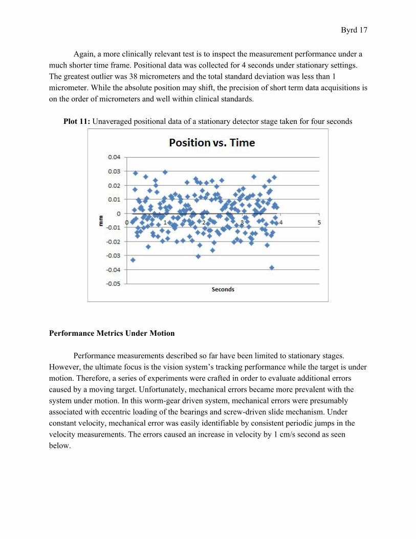
Again, a more clinically relevant test is to inspect the measurement performance under a much shorter time frame. Positional data was collected for 4 seconds under stationary settings. The greatest outlier was 38 micrometers and the total standard deviation was less than 1 micrometer. While the absolute position may shift, the precision of short term data acquisitions is on the order of micrometers and well within clinical standards.

Plot 11: Unaveraged positional data of a stationary detector stage taken for four seconds

Performance Metrics Under Motion

Performance measurements described so far have been limited to stationary stages.

However, the ultimate focus is the vision system’s tracking performance while the target is under motion. Therefore, a series of experiments were crafted in order to evaluate additional errors caused by a moving target. Unfortunately, mechanical errors became more prevalent with the system under motion. In this worm-gear driven system, mechanical errors were presumably associated with eccentric loading of the bearings and screw-driven slide mechanism. Under constant velocity, mechanical error was easily identifiable by consistent periodic jumps in the velocity measurements. The errors caused an increase in velocity by 1 cm/s second as seen below.

Byrd 18

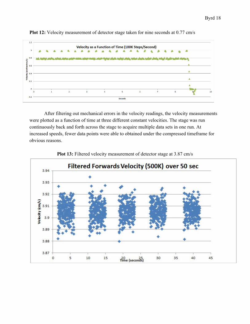
Plot 12: Velocity measurement of detector stage taken for nine seconds at 0.77 cm/s

After filtering out mechanical errors in the velocity readings, the velocity measurements were plotted as a function of time at three different constant velocities. The stage was run continuously back and forth across the stage to acquire multiple data sets in one run. At increased speeds, fewer data points were able to obtained under the compressed timeframe for obvious reasons.

Plot 13: Filtered velocity measurement of detector stage at 3.87 cm/s

Byrd 19

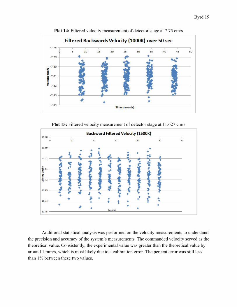
Plot 14: Filtered velocity measurement of detector stage at 7.75 cm/s

Plot 15: Filtered velocity measurement of detector stage at 11.627 cm/s

Additional statistical analysis was performed on the velocity measurements to understand

the precision and accuracy of the system’s measurements. The commanded velocity served as the theoretical value. Consistently, the experimental value was greater than the theoretical value by around 1 mm/s, which is most likely due to a calibration error. The percent error was still less than 1% between these two values.

Byrd 20

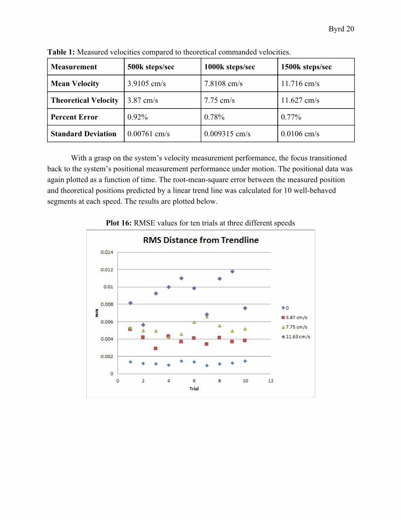
Table 1: Measured velocities compared to theoretical commanded velocities.

Measurement 500k steps/sec 1000k steps/sec 1500k steps/sec

Mean Velocity 3.9105 cm/s 7.8108 cm/s 11.716 cm/s

Theoretical Velocity 3.87 cm/s 7.75 cm/s 11.627 cm/s

Percent Error 0.92% 0.78% 0.77%

Standard Deviation 0.00761 cm/s 0.009315 cm/s 0.0106 cm/s

With a grasp on the system’s velocity measurement performance, the focus transitioned

back to the system’s positional measurement performance under motion. The positional data was again plotted as a function of time. The root-mean-square error between the measured position and theoretical positions predicted by a linear trend line was calculated for 10 well-behaved segments at each speed. The results are plotted below.

Plot 16: RMSE values for ten trials at three different speeds

Byrd 21

7. Discussion and Conclusions The biggest experimental challenge was not having a clearly defined control with which

to compare experimental results with. There was no perfect measuring system. By comparing samples amongst each other, the system’s precision was easily examined. Assessing the vision system’s accuracy required alternative approaches. With no known absolute positions, it was only possible to compare relative positions amongst each other. The SmartMotor’s stepping capability allowed for very controlled transitions and velocities. However, this prototype was encumbered by mechanical errors which affected the consistency of its performance.

By testing for consistency in uniform transitions, it was confirmed that the motor’s stepping system performed well across the entire stage. The standard deviation amongst measured transitions was 10.49 micrometers. The mean measured distance was 45 micrometers larger than the commanded transition. This offset is believed to be caused by calibration. Nonetheless, the measured transitions of the stage as it moved matched the SmartMotor’s commanded movements within 100 micrometers. This experiment verified the assumption that the commanded motor movements could serve as a reliable control.

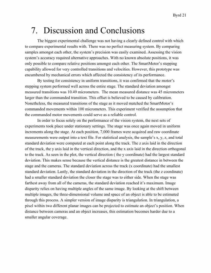
In order to focus solely on the performance of the vision system, the next sets of experiments took place under stationary settings. The stage was once again moved in uniform increments along the stage. At each position, 7,000 frames were acquired and raw coordinate measurements were output into a text file. For statistical analysis, the sample’s x, y, z, and total standard deviation were computed at each point along the track. The z axis laid in the direction of the track, the y axis laid in the vertical direction, and the x axis laid in the direction orthogonal to the track. As seen in the plot, the vertical direction ( the y coordinate) had the largest standard deviation. This makes sense because the vertical distance is the greatest distance in between the stage and the cameras. The standard deviation across the track (x coordinate) had the smallest standard deviation. Lastly, the standard deviation in the direction of the track (the z coordinate) had a smaller standard deviation the closer the stage was to either side. When the stage was farthest away from all of the cameras, the standard deviation reached it’s maximum. Image disparity relies on having multiple angles of the same image. By looking at the shift between multiple images, the three-dimensional volume and space of an object is able to be estimated through this process. A simpler version of image disparity is triangulation. In triangulation, a pixel within two different planar images can be projected to estimate an object’s position. When distance between cameras and an object increases, this estimation becomes harder due to a smaller angular coverage.

Byrd 22

Figure 6: Effects of distance on triangulation positional approximation method

This positional performance dependent on spatial coverage is an important consideration

when increasing the size of this system to an entire room. The more angles covered within the room, the greater positional performance will be. However, the exact relationship between camera positioning and positional performance is not yet quantifiable. The next step in testing for spatial dependence will be to simulate a clinical room. By placing cameras in the corners of a 6’x 6’ room, it will be possible to understand what the implication of this effect are on a large scale.

The next subject of interest was how the system performed over time. To test for this, positional information of a stationary stage was acquired for an hour. 10 frames samples were continuously collected and analyzed. Each sample mean was plotted as a function of time throughout the entire run. A noticeable exponential decay was observed as the positional reading dropped 200 µm. It was as if the positional readings were settling with very large time constant. To further explore this, the same experiment was done at three additional locations and the same logarithmic decay was seen at all three positions.

It is important to note that an hour image acquisition is unreasonable within the clinical setting. Therefore, it does not matter as much that the positional readings are shifting so much over an hour. In a clinical setting, the tracking system must be able to perform equally as well each time the clinician starts tracking a patient. To test for consistency in positional readings upon multiple start-ups, the vision system was run for 10 seconds as 10 count samples were collected. Then the vision system was turned off for 10 seconds, and ran for 10 seconds. By collecting 10 count samples 10 seconds apart, it was possible to see the positional readings shift by 1-2 µm in each run. Since this much shifting happened when the data acquisitions were taken so closely in time, I was interested in seeing how much the reported position would change over a longer period. Therefore, another data acquisition took place 2 hours the first data acquisition. Between the two hours, the reported position of the stationary stage shifted by 60 µm. It is possible that environmental disturbances could have caused these shifts on the level of micrometers. Through extensive testing in an imperfect testing condition, the largest shift in reported position was still under 300 µm.

While the precision remained under 1 µm in each individual sample, the sample’s position drifts over time. Using the vision system alone, an absolute reference point cannot be determined. Therefore, there exists the need for an additional fiducial marker with a known

Byrd 23

geographical locations. Much like how a GPS system works, the vision system can use this reference to correct for possible offsets.

Up until now, the positional data points have been averaged in some way. While these sampled means are useful in identifying position-dependent and time-dependent performance relationships, an inherent lag is caused by averaging frames together. To minimize lag time, positional data must be collected as close to real-time as possible. Therefore, it is of interest whether or not raw positional data points can be used instead of averaged sample means.

To test for this, unaveraged positional data of both the detector stand and the target stage was recorded and analyzed over the course of an hour. As seen in Plot 10, the biggest outlier was 3 mm out of 170,000 points which is too large of an error to exist for proper image reconstruction. The disturbances in the positional readings appeared to occur at the same time for both the detector stage and the target stage. This leads one to think that an environmental disturbance could have caused these momentary fluctuations seen in the plot.

As stated before, performance within a short time scale is much more important than performance over a long time scale in the clinic. The positional data that was taken in 4 seconds has a far greater precision, with the greatest outlier being 38 micrometers and the total standard deviation being less than 1 µm. While the absolute position may shift, the vision system is able to produce precision on the level of micrometers. The outliers seen in the raw data points were typically groupings of one or two misbehaving data points. Therefore, sampling of a couple points may help reduce these outliers without introducing significant lag into the system.

The experimentation transitioned towards making measurement with the detector stage in motion. The stage was moved at a constant velocity across the stage as measures of instantaneous velocity were output to a data file. With these measurements, a clear mechanical error was identified. Every second, a 1 cm/s jump in velocity is seen. This periodic jump is consistent and only appears in experiments with mechanical movements. Therefore, this error has been identified as purely mechanical. To focus more on the vision system error, the mechanical errors need to be filtered out. When inspecting velocity, this is easy to do by taking out all velocity measurements which are drastically higher and occur periodically. When this filtering process was complete, the actual velocity measurement errors could be further inspected. The filtered velocity values for three different speeds can be seen in Plots 13-15. Obviously, at higher speeds there were less data points collected in each run. At each speed, the measured velocity appears to be 0.1 cm/s higher than the commanded velocity. The percent error in between the commanded velocity and the measured velocity was still under 1% at all speeds. As expected, the spread in measured velocities was slightly greater at higher speeds. Nonetheless, all standard deviations in velocity were under 0.1 mm/s.

The matter of most interest within this project is understanding how the vision system’s measurement performance is affected by motion. If the vision system could not perform well with a moving target, then the RoomPET project could not use this vision system in the final system. Fortunately, the results indicate high performance in positional measurements at low

Byrd 24

constant-velocities. Due to the mechanical system constraints, only velocities below 20 cm/s could be inspected.

After fitting the ‘well-behaved’ positional data with linear trendlines and inspecting the RMS error in 10 different trials at three different speeds, the higher velocities have a higher RMS error as expected. At zero velocity, the stage obviously has the lowest RMS error. The RMS error increases with velocity. Overall, the RMS error was under 15 µm in all experimental trials. From this, it can be concluded that velocity has negligible effect on positional measurement performance at low constant velocities.

Since many of the positional estimation computations were done internally in a “black box” software, certain inconsistencies were observed without a clear source of error. Certain errors may have been introduced in the initial calibration or by the dynamics of the internal Kalman filter algorithm. From all experimentation, the most important conclusion is that all errors combined are still under 300 µm. This incredibly precise tracking system has great potential to be used for in the final brain PET system. While the system cannot identify absolute position accurately, an external geographical marker can assist in correcting the drifting positional readings.

The results found confirm the two main hypotheses. First, tracking performance is dependent on spatial positioning with respect to the cameras. Secondly, tracking performance is dependent on the velocity at which the target is moving. An additional discrepancy was found which causes for a shifting effect to occur over long periods of time. The relative distance between items can be very precisely and accurately measured, however determining the absolute position is challenging without a known geographical reference outside of the IR tracking system. Moving forward, all errors found in this study were small enough to not be a concern in the clinical application. The limiting resolution will be dependent on the PET detector, not the tracking system.

While the mechanics of the low-cost prototype inhibit the future implications of these specific results, the prototype still provides a strong proof of principle. It supports the idea that IR vision systems could be used within the realm of dynamic imaging. By providing accuracy on the level of micrometers, this type of system outperforms many current tracking systems. The prototype also provides a platform for the testing and optimization of predictive tracking algorithms.

An important outcome from this set of measurements was to establish techniques, approaches and language of this type of system, so that when another system is built for the brain RoomPET that we understand how to handle similar problems that arise. A protocol for testing such a system as well as the framework for discussing errors has also been established through this project.

Byrd 25

8. Appendices

I. Blueprints of Fabricated Components

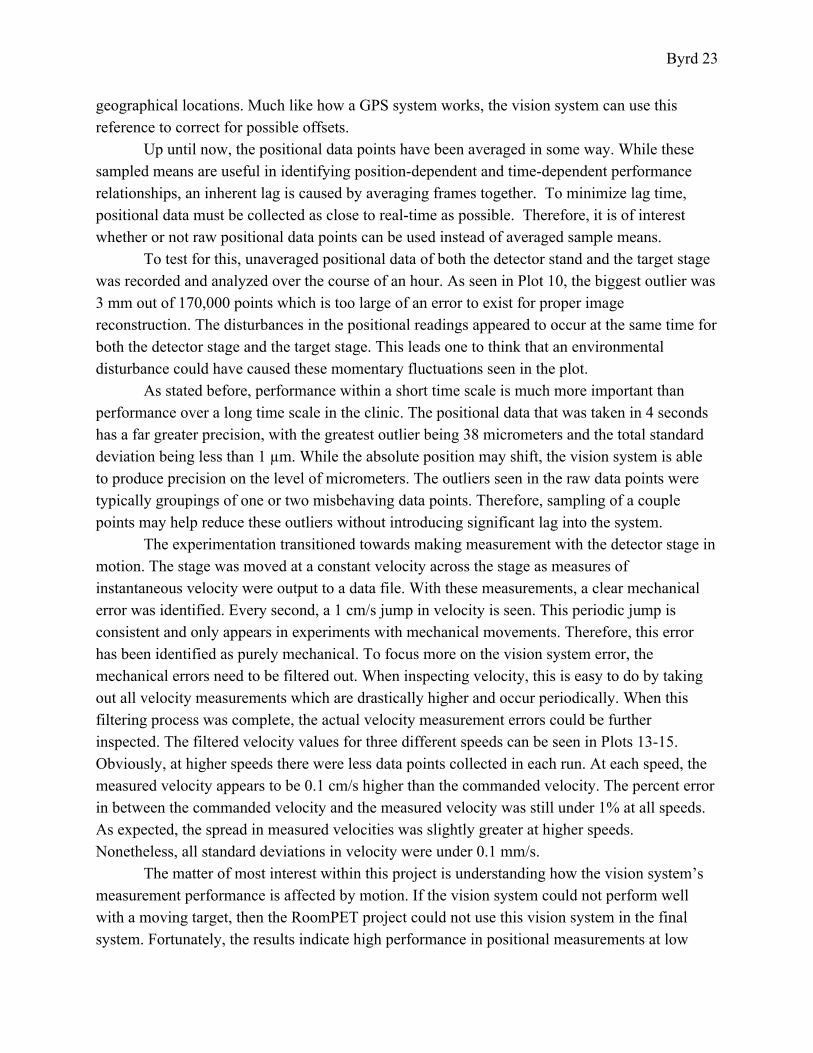
Blueprint 1: Wire clip (Dimensions in mm)

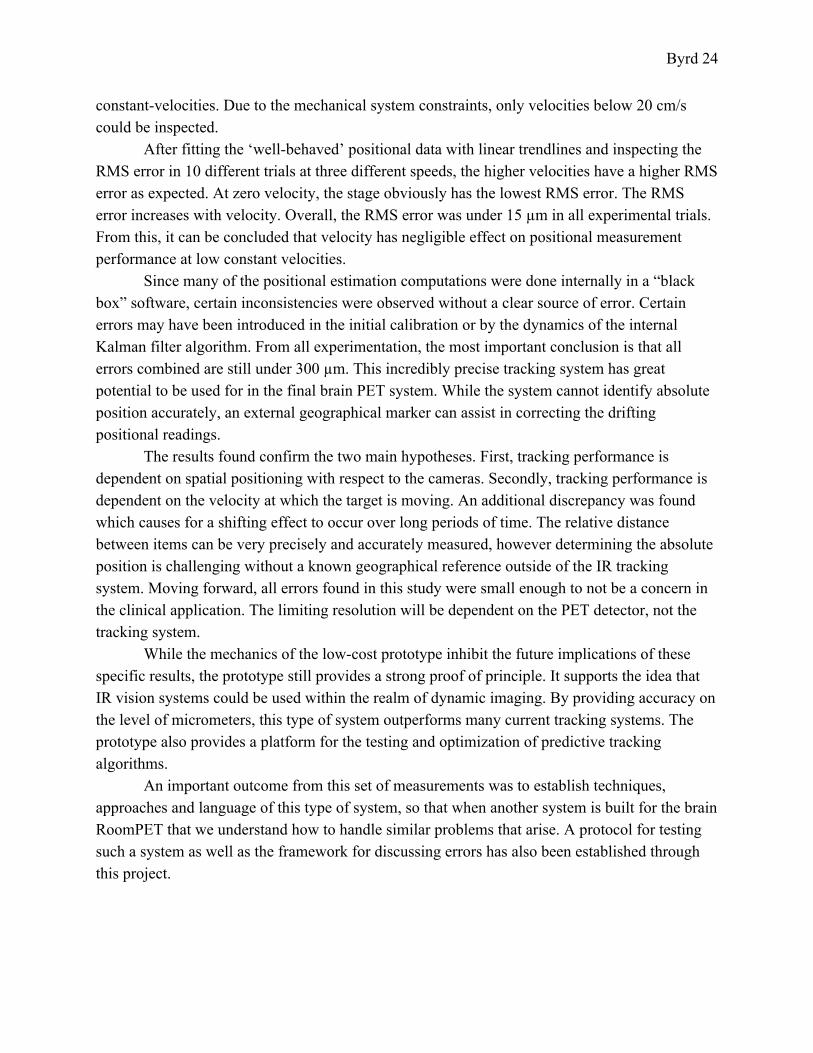
Blueprint 2: IR Camera Bracket (Dimensions in mm)

Byrd 26

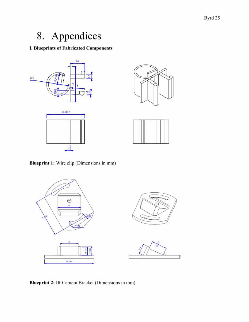
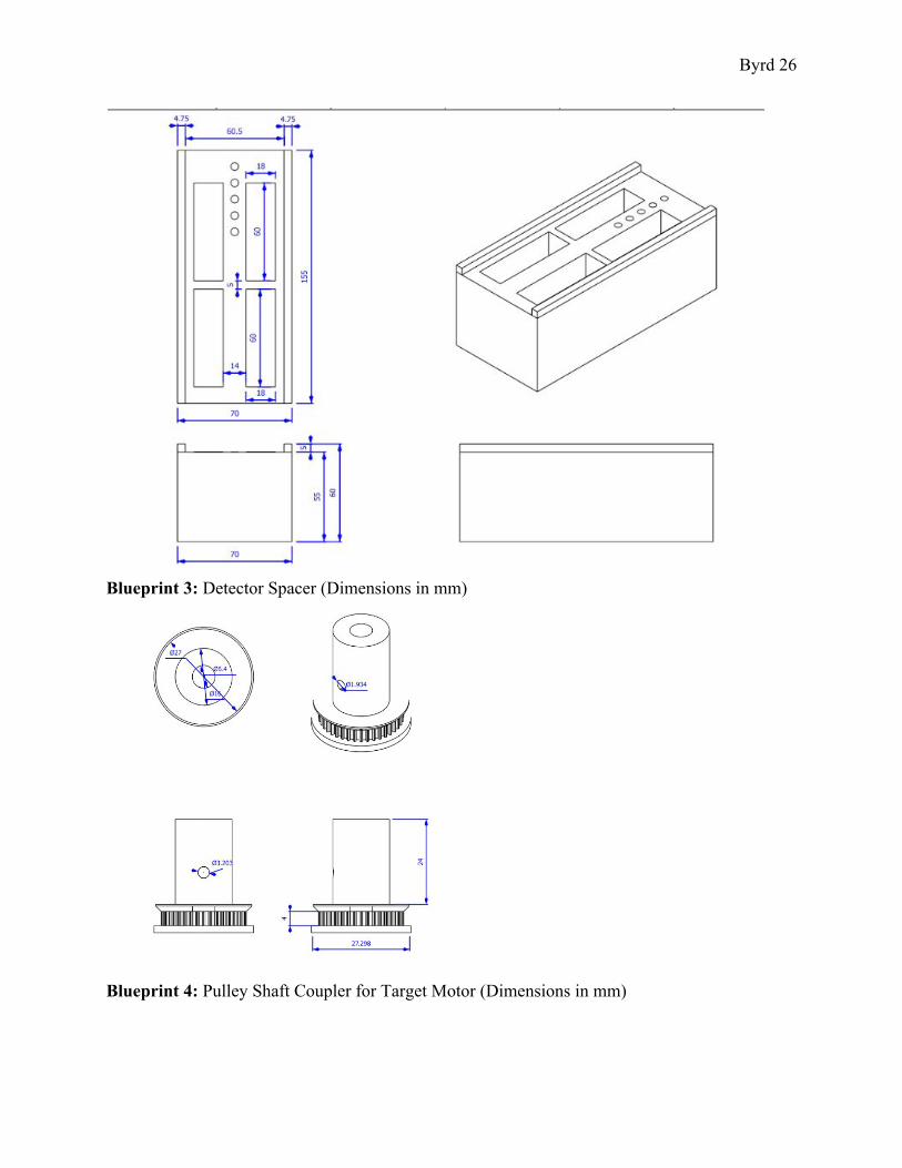
Blueprint 3: Detector Spacer (Dimensions in mm)

Blueprint 4: Pulley Shaft Coupler for Target Motor (Dimensions in mm)

Byrd 27

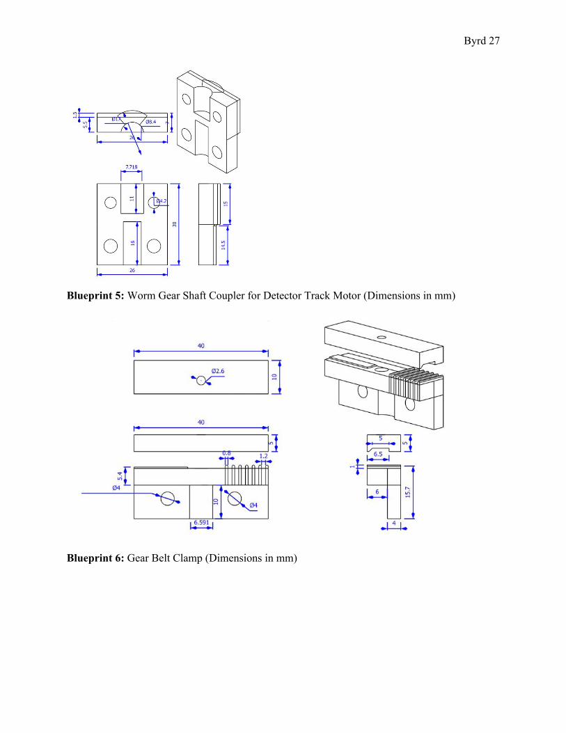
Blueprint 5: Worm Gear Shaft Coupler for Detector Track Motor (Dimensions in mm)

Blueprint 6: Gear Belt Clamp (Dimensions in mm)

Byrd 28

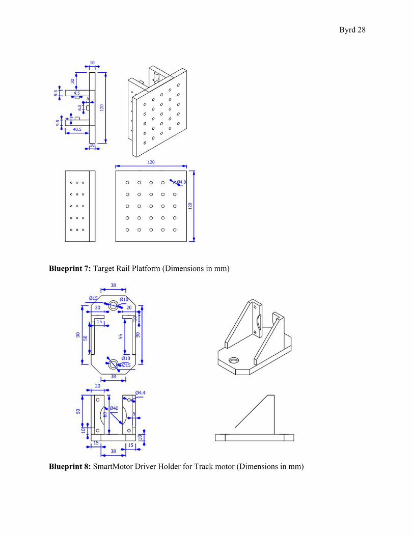
Blueprint 7: Target Rail Platform (Dimensions in mm)

Blueprint 8: SmartMotor Driver Holder for Track motor (Dimensions in mm)

Byrd 29

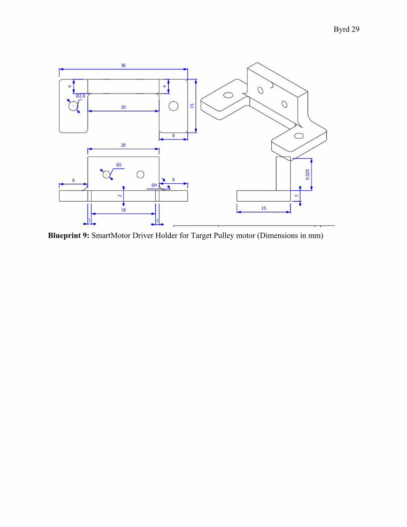
Blueprint 9: SmartMotor Driver Holder for Target Pulley motor (Dimensions in mm)

Byrd 30

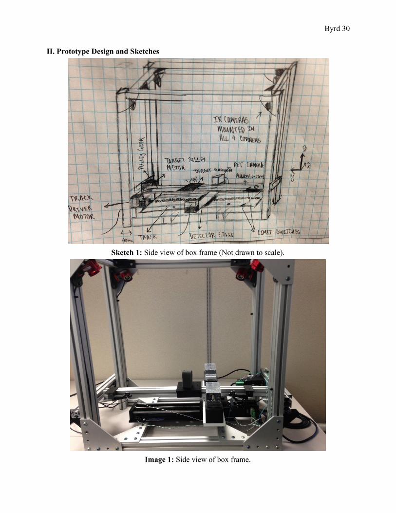
II. Prototype Design and Sketches

Sketch 1: Side view of box frame (Not drawn to scale).

Image 1: Side view of box frame.

Byrd 31

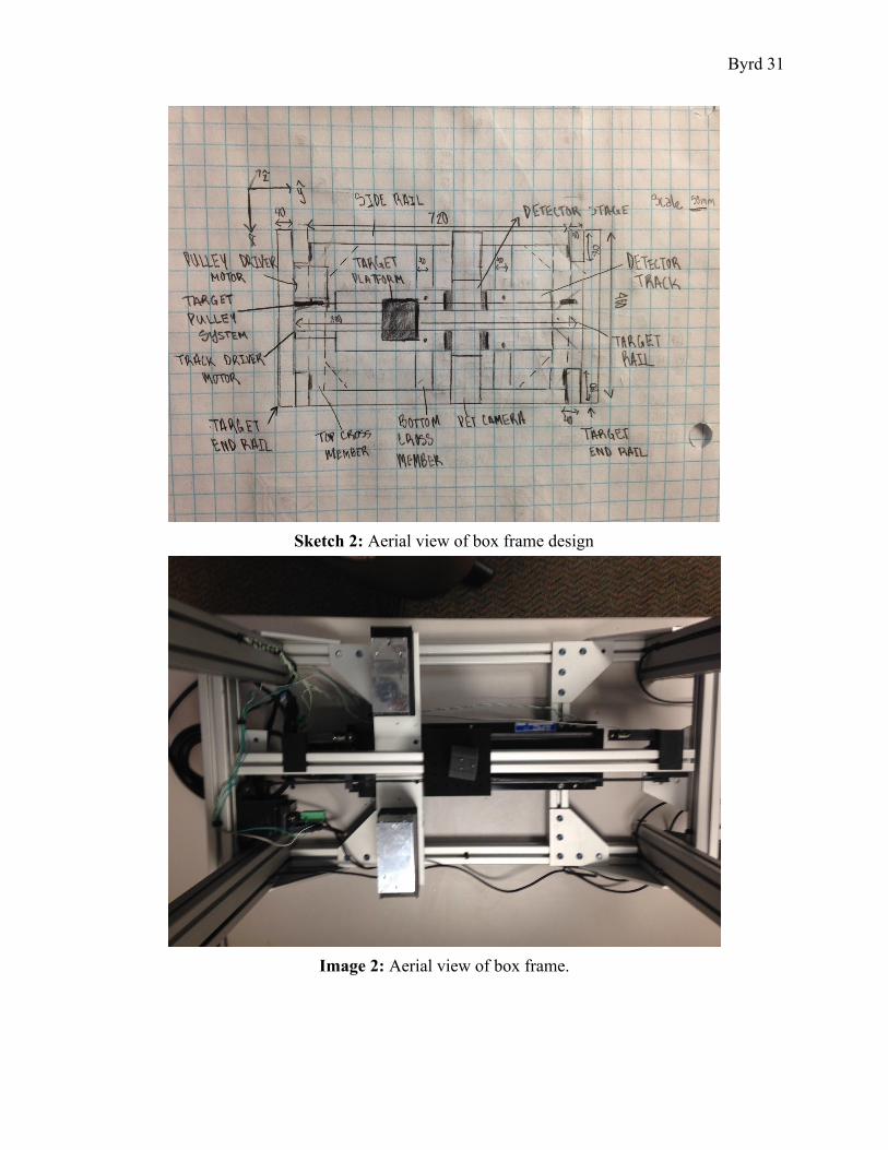
Sketch 2: Aerial view of box frame design

Image 2: Aerial view of box frame.

Byrd 32

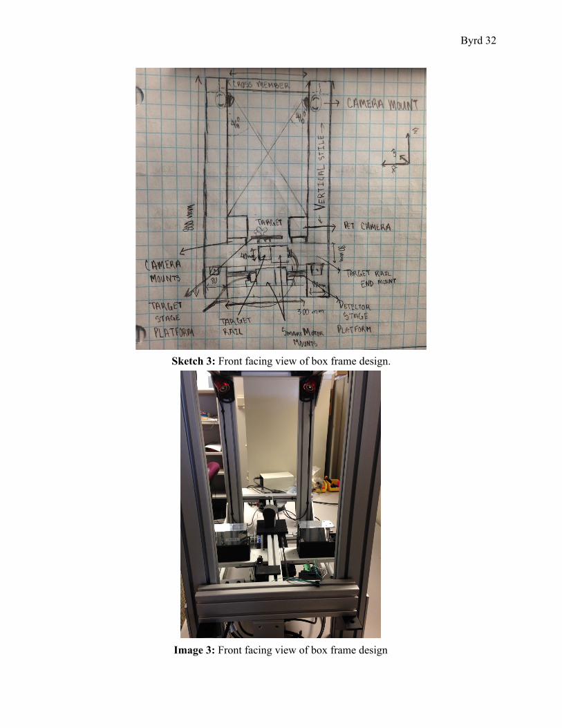
Sketch 3: Front facing view of box frame design.

Image 3: Front facing view of box frame design

Byrd 33

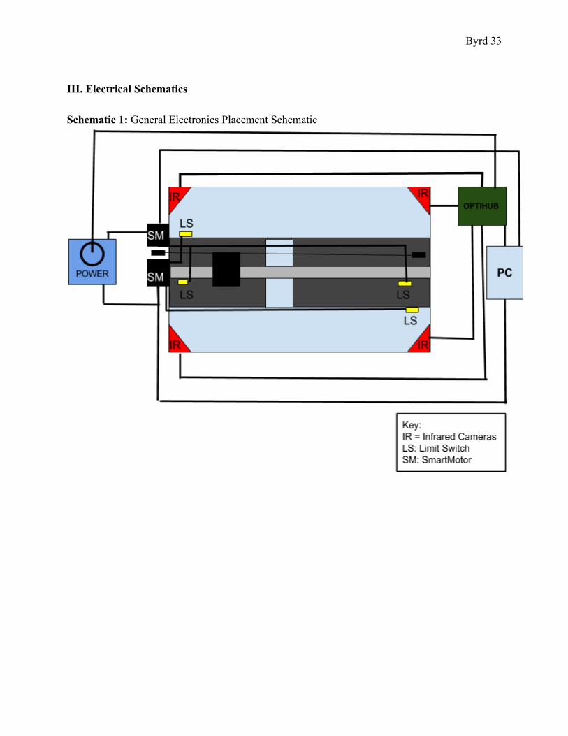
III. Electrical Schematics Schematic 1: General Electronics Placement Schematic

Byrd 34

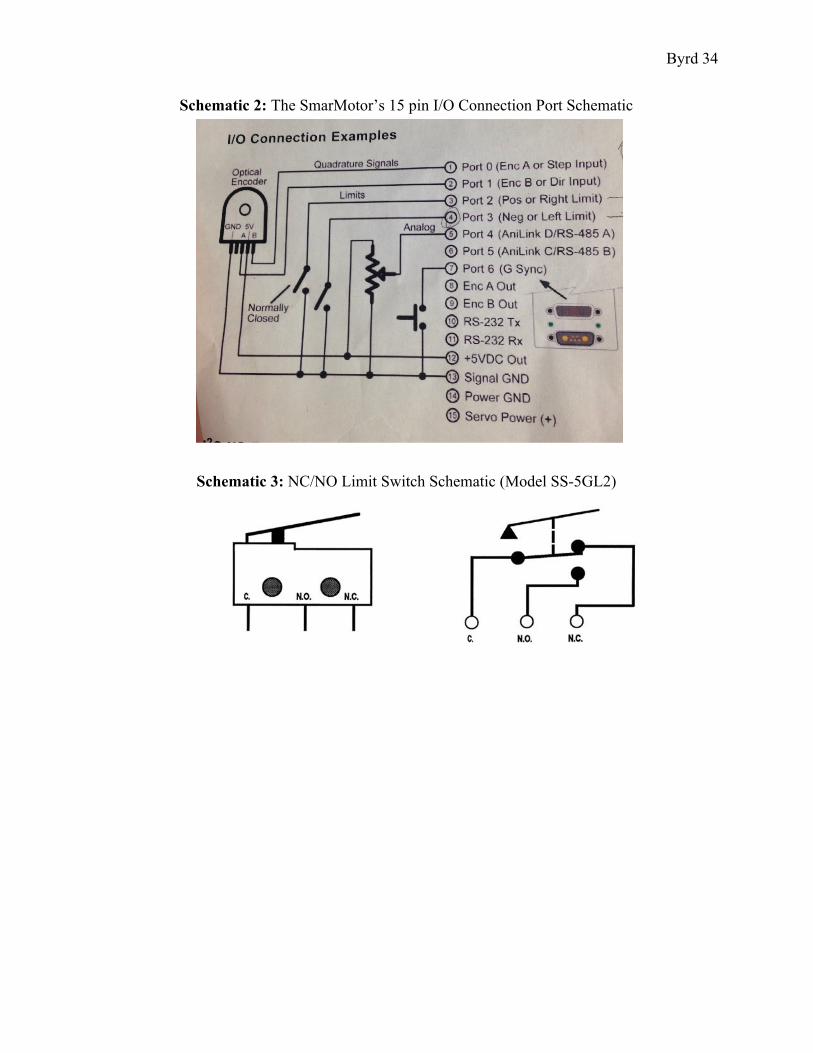
Schematic 2: The SmarMotor’s 15 pin I/O Connection Port Schematic

Schematic 3: NC/NO Limit Switch Schematic (Model SS-5GL2)

Byrd 35

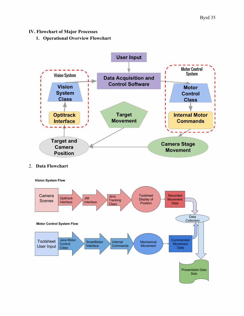
IV. Flowchart of Major Processes 1. Operational Overview Flowchart

2. Data Flowchart

Byrd 36

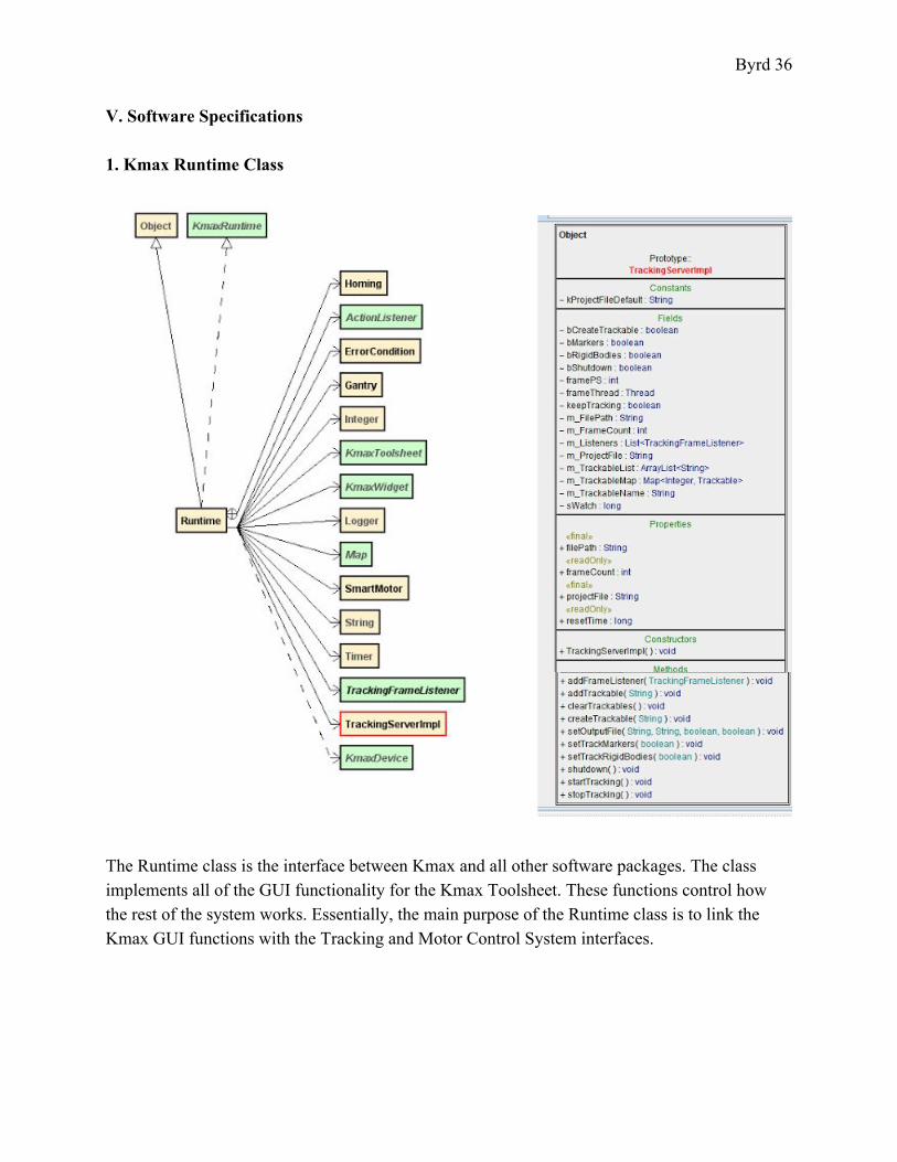
V. Software Specifications 1. Kmax Runtime Class

The Runtime class is the interface between Kmax and all other software packages. The class implements all of the GUI functionality for the Kmax Toolsheet. These functions control how the rest of the system works. Essentially, the main purpose of the Runtime class is to link the Kmax GUI functions with the Tracking and Motor Control System interfaces.

Byrd 37

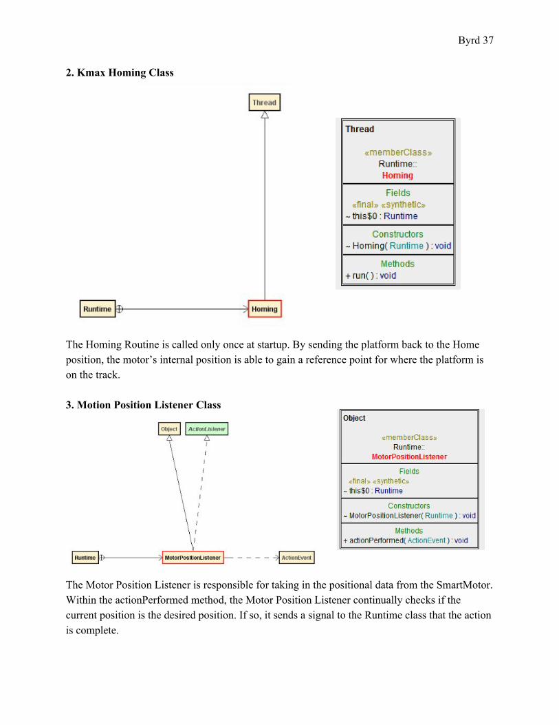
2. Kmax Homing Class

The Homing Routine is called only once at startup. By sending the platform back to the Home position, the motor’s internal position is able to gain a reference point for where the platform is on the track. 3. Motion Position Listener Class

The Motor Position Listener is responsible for taking in the positional data from the SmartMotor. Within the actionPerformed method, the Motor Position Listener continually checks if the current position is the desired position. If so, it sends a signal to the Runtime class that the action is complete.

Byrd 38

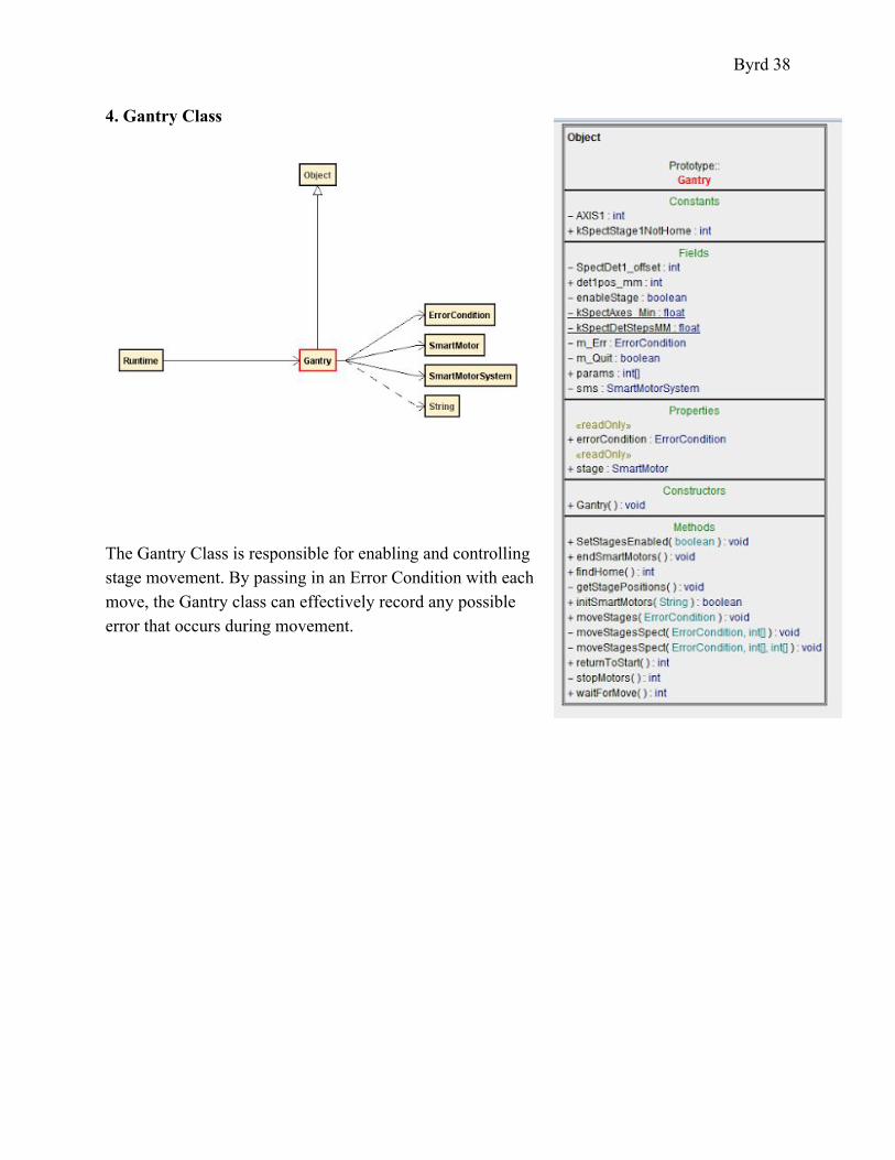
4. Gantry Class

The Gantry Class is responsible for enabling and controlling stage movement. By passing in an Error Condition with each move, the Gantry class can effectively record any possible error that occurs during movement.

Byrd 39

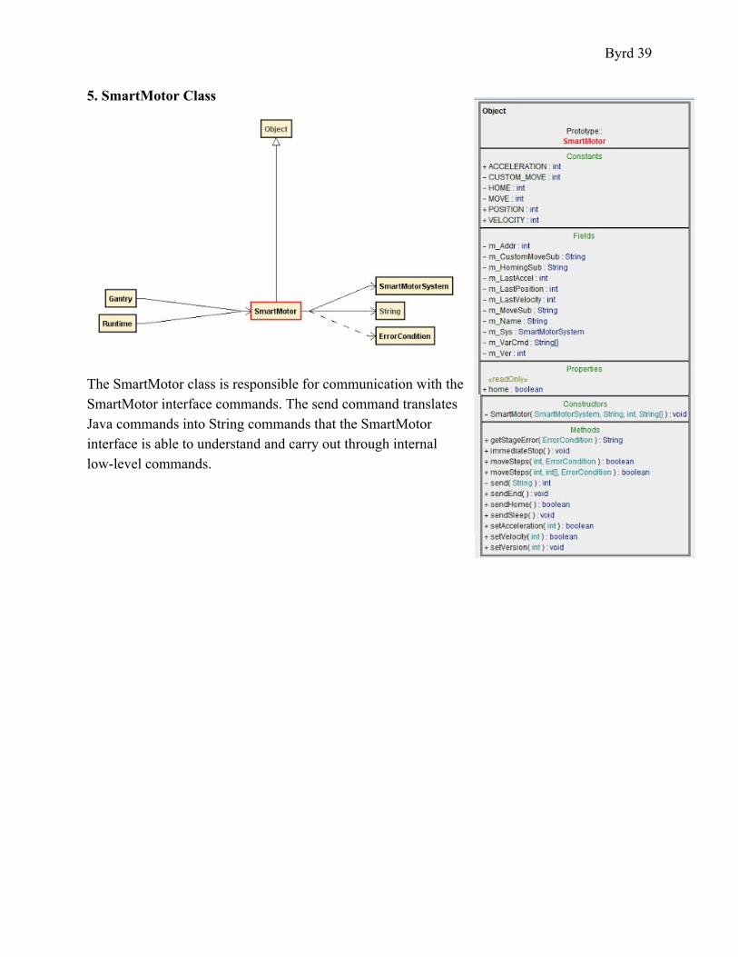
5. SmartMotor Class

The SmartMotor class is responsible for communication with the SmartMotor interface commands. The send command translates Java commands into String commands that the SmartMotor interface is able to understand and carry out through internal low-level commands.

Byrd 40

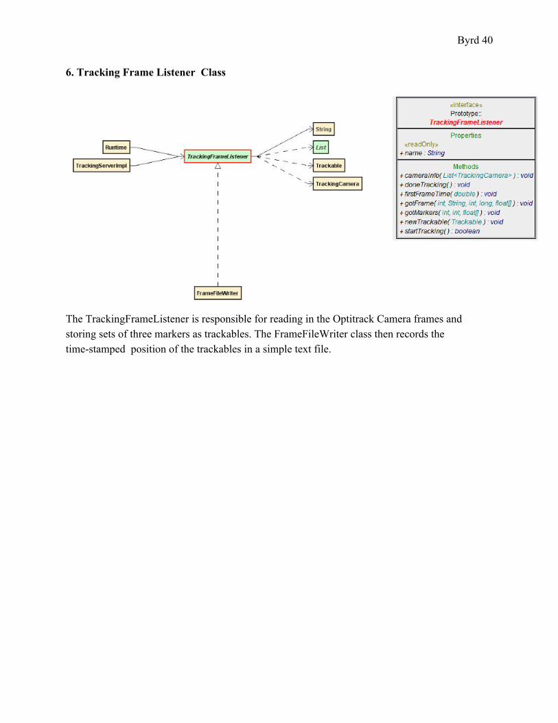
6. Tracking Frame Listener Class

The TrackingFrameListener is responsible for reading in the Optitrack Camera frames and storing sets of three markers as trackables. The FrameFileWriter class then records the time-stamped position of the trackables in a simple text file.

Byrd 41

VI. SmartMotor Control System Command Routines

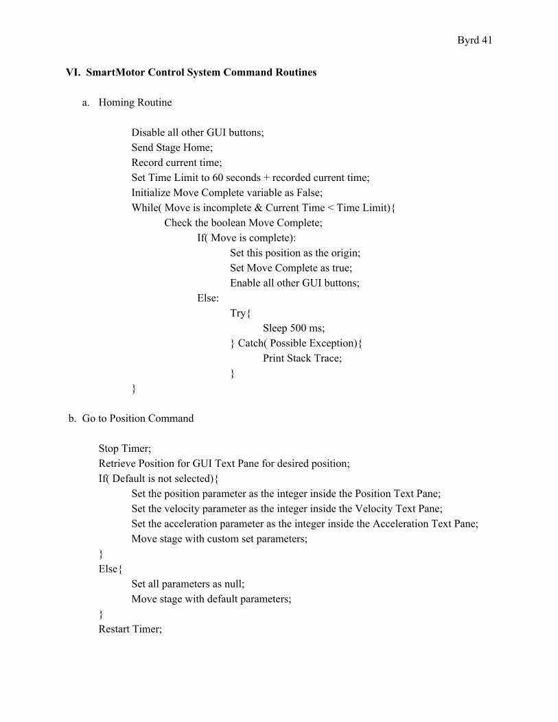
a. Homing Routine Disable all other GUI buttons; Send Stage Home; Record current time; Set Time Limit to 60 seconds + recorded current time; Initialize Move Complete variable as False; While( Move is incomplete & Current Time < Time Limit){

Check the boolean Move Complete; If( Move is complete):

Set this position as the origin; Set Move Complete as true; Enable all other GUI buttons;

Else: Try{

Sleep 500 ms; } Catch( Possible Exception){ Print Stack Trace; }

}

b. Go to Position Command

Stop Timer; Retrieve Position for GUI Text Pane for desired position; If( Default is not selected){

Set the position parameter as the integer inside the Position Text Pane; Set the velocity parameter as the integer inside the Velocity Text Pane; Set the acceleration parameter as the integer inside the Acceleration Text Pane; Move stage with custom set parameters;

} Else{

Set all parameters as null; Move stage with default parameters;

} Restart Timer;

Byrd 42

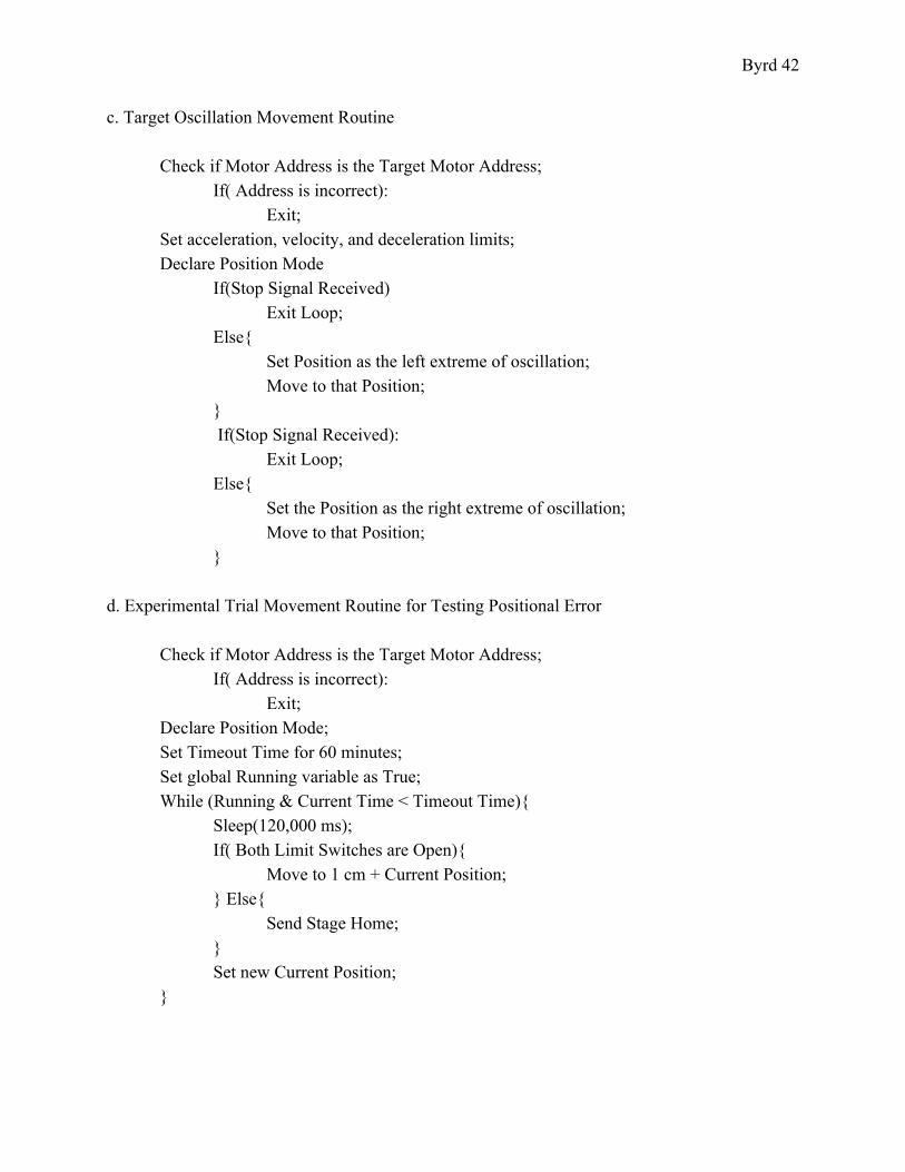
c. Target Oscillation Movement Routine Check if Motor Address is the Target Motor Address;

If( Address is incorrect): Exit;

Set acceleration, velocity, and deceleration limits; Declare Position Mode

If(Stop Signal Received) Exit Loop;

Else{ Set Position as the left extreme of oscillation; Move to that Position;

} If(Stop Signal Received):

Exit Loop; Else{

Set the Position as the right extreme of oscillation; Move to that Position;

} d. Experimental Trial Movement Routine for Testing Positional Error

Check if Motor Address is the Target Motor Address;

If( Address is incorrect): Exit;

Declare Position Mode; Set Timeout Time for 60 minutes; Set global Running variable as True; While (Running & Current Time < Timeout Time){

Sleep(120,000 ms); If( Both Limit Switches are Open){

Move to 1 cm + Current Position; } Else{

Send Stage Home; } Set new Current Position;

}

Byrd 43

e. Experimental Trial Movement Routine for Testing Error at Constant Velocity Check if Motor Address is the Target Motor Address;

If( Address is incorrect): Exit;

Set acceleration, velocity, and deceleration limits; Set Timeout Time for 10 minutes; Set global Running variable as True; While (Running & Current System Time < Timeout Time){

If( Moving is Enabled){ ***//Velocity Mode Runs Motor at Constant Velocity Declare Velocity Mode;

} Else{ Send Stage Home; Sleep(30,000 ms); Enable Moving again;

} }

f. Experimental Trial Movement Routine for Testing Error at Constant Acceleration

Check if Motor Address is the Target Motor Address;

If( Address is incorrect): Exit;

Set acceleration, velocity, and deceleration limits; Set Timeout Time for 10 minutes; Set Running variable as True; While (Running & Current System Time < Timeout Time){

If( Moving is Enabled){ ***// Acceleration Mode Runs Motor at Constant Velocity Declare Acceleration Mode;

} Else{ Send Stage Home; Sleep(30,000 ms); Enable Moving again;

} }

Byrd 44

9. Bibliography

Animatics. (2016). SmartMotorTM Developer’s Guide. Springfield, PA. Moog Inc. McKisson, J (2017) TrackingKinematics [Unpublished code]. Newport News, VA: Thomas aaaaaaJefferson Laboratory. Optitrack. (2016). Motive API. Retrieved from http://wiki.optitrack.com Smith, M. (2016). Specific aims: Natural environment brain imaging with a RoomPET aaaaaaScanner. (Unpublished document). University of Maryland, Baltimore, MD. Sparrow Corporation. (2016). Kmax Manual 10.1. Port Orange, FL: Author.

Weisenberger, A. G., et al. (2008). Awake animal SPECT: Overview and initial results. 2008 aaaaaaIEEE Nuclear Science Symposium Conference Record. Dresden, Germany.