University of Southern Queensland

Faculty of Health, Engineering and Sciences

3D Modelling for surveying projects using Unmanned Arial Vehicles

(UAVs) and Laser Scanning

A dissertation submitted by

Bradley Redding

in fulfilment of the requirements of

ENG4111 and 4112 Research Project

towards the degree of

Bachelor of Spatial Science (Honours) (Surveying)

Submitted October, 2016

i

Table of Contents List of Figures iv

List of Tables iv

Abstract vii

Chapter 1 - Introduction 1

1.1 Project Background 1 1.2 Statement of Problem 1 1.3 Project Justification 2 1.4 Project Aim 2 1.5 Project Objectives 2 1.6 Structure of Dissertation 3

Chapter 2 - Literature Review 4

2.1 Photogrammetry 4 2.1.1 Overview 4 2.2 Applications 4 2.3 Triangulation 5 2.4 Surface Construction & Feature Extraction 5 2.5 Sensors 6 2.6 Processing Software 6 2.6.1 Survey Data Processing 6 2.6.2 Pix4D 6 2.7 Limitations of Photogrammetry 7 2.8 Base to Height Ratio 8 2.9 UAV Accuracy- Past Results Analysis 8 2.9.1 Aerial Survey – Veio Italy 8 2.9.2 Topographic Survey - NSW Australia 9 2.9.3 Summary 10 2.10 Portrait V’s Landscape Accuracy 11 2.11 Time and Cost Analysis 12 2.12 Terrestrial Photogrammetry 13 2.13 Oblique UAV Photogrammetry. 13 2.14 Unmanned Arial Vehicles 13 2.15 Types & Industry standards 14 2.16 Licencing 16 2.17 Scanning (for comparison) 16

Chapter 3 - Method 17

3.1 Introduction 17 3.2 Design Considerations 17 3.2.1 Sensor & Settings 17 3.2.2 Camera Stabilisation (Gimbal) 18 3.2.3 Apparent Image Motion (AIM) 18 3.2.4 Platform 18 3.3 Location 19

ii

3.3.1 Control Network 19 3.3.2 Coordinate System 19 3.4 Field Testing Procedure 20 3.4.1 Overview 20 3.5 20 3.5.1 Traditional Surveying 20 3.6 UAV Photogrammetry 21 3.6.1 Targets 21 3.6.2 Front & Side Overlap 21 3.6.3 Flight Operation & Flight Path 22 3.7 Simulations 22 3.7.1 Flight Time & Portrait v’s Landscape Efficiency Simulation 22 3.8 Process 23 3.8.1 Processing Efficiency Simulation 23 3.9 Terrestrial Photogrammetry 24 3.10 Scanning 24 3.11 Targets 24 3.12 Data Storage 24 3.13 Processing, Comparison & Analysis 24 3.13.1 Data Processing 24 3.13.2 Preliminarily Processing 25 3.13.3 Traditional Surveying and Control Network Processing 25 3.13.4 Photogrammetric Processing (Pix4D) 25 3.13.5 Process Scanning Data 26 3.13.6 Process Terrestrial Photogrammetry 26 3.14 Photogrammetry Processing 27 3.14.1 Scanner Processing 27 3.14.2 Survey, Photogrammetric and Scan Data Comparison Process 27 3.15 Data analysis 29

Chapter 4 - Results 30

4.1 Introduction 30 4.2 Simulation 30 4.3 Accuracy Analysis 30 4.4 Flight Time Analysis 31 4.5 Processing Time analysis 31 4.5.1 Processing Without Control 31 4.5.2 Processing with Control 31 4.6 Results - Airborne Photogrammetry Quality Report Analysis. 32 4.6.1 Coverage Percentage 32 4.6.2 Flat Surfaces 32 4.6.3 Textured Surfaces 32 4.6.4 Point Accuracy Survey Data Comparison 32 4.6.5 Point Accuracy Scanning Data Comparison 32 4.7 Accuracy Analysis from Quality Reports 32 4.7.1 Average Ground Sampling Distance (GSD) 33 4.7.2 Images Captured 33

iii

4.7.3 Images Useable 33 4.7.4 Calibrated Images 33 4.7.5 Area Covered by Flight (Hectares) 34 4.7.6 Number of Images Per Hectare 34 4.7.7 Number of Points Per Hectare 34 4.7.8 Matched Points 34 4.7.9 Geo-referencing Error 34 4.7.10 Image Overlap 35 4.7.11 Control Network 36 4.1 Surface Comparison 37 4.2 Area 1 & 4 Driveway as well as Driveway and Grass 39 4.3 Areas 2 and 5 40 4.4 Area 3 Short Grass 41 4.5 Surfaces Summary 41 4.6 Results Ground Based Photogrammetry 42

Chapter 5 - Discussion 43

5.1 Introduction 43 5.1.1 Area 1 & 4 –Discussion 43 5.1.2 Areas 2 and 5 Discussion 43 5.1.3 Area 3 –Discussion 43 5.1.4 Surfaces Summary Discussion 44 5.1.5 Shadows 44 45 5.2 Model Completeness & Visual discussion 46 5.3 Case 1: Building N/S 46 5.4 Case 2 : NE Building 47 5.5 Case 3- Building NE/SSW (diagonal to run lines) 48 5.6 Case 4 – Overgrown and Dense Foliage Area 49 5.7 Case 5 – Ground surface Coverage in Dense Trees 50 5.8 Model Completeness & visual discussion conclusion 51 5.8.1 Summary Table 51 5.8.2 Why does Portrait Capture Some Areas Otherwise Missed by

Landscape? 51 5.8.3 Camera Orientation Practicality 53

Chapter 6 Conclusion 54

6.1.1 Findings 54 6.1.2 Testing Limitations 54 6.2 Further Research 55 6.2.1 Research 1 55 6.2.2 Research 2 55 6.2.3 Research 3 55

Bibliography 57

Appendix A 59

Appendix B 60

iv

List of Figures

Figure 2.1 - Processing Software Accuracy ................................................................................. 7 Figure 2.2 - Landscape ............................................................................................................... 11 Figure 2.3 - Landscape ............................................................................................................... 11 Figure 2.4 - Triangulation (Stojakovie) ....................................................................................... 13 Figure 3.1 - Gimbal & Camera ................................................................................................... 18 Figure 3.2 - Workflow ................................................................................................................. 20 Figure 3.3 - Clear Image ............................................................................................................. 25 Figure 3.4 - Image Blur .............................................................................................................. 25 Figure 4.1 - Landscape Photo Coverage .................................................................................... 35 Figure 4.2 - Portrait Photo Coverage .......................................................................................... 35 Figure 4.3 - Control Network ...................................................................................................... 36 Figure 4.4 - Portrait Control Summary ....................................................................................... 36 Figure 4.5 - Landscape Control Summary ................................................................................. 36 Figure 4.6 - Control Error ......................................................................................................... 37 Figure 4.7 - Area Overview ......................................................................................................... 38 Figure 4.8 - Area 1 Statistics ....................................................................................................... 39 Figure 4.9 - Area 2 Statistics ....................................................................................................... 39 Figure 4.10 - Area 5 Statistics ..................................................................................................... 40 Figure 4.11 - Area 2 Statistics ................................................................................................... 40 Figure 4.12 - Area 3 Statistics ................................................................................................... 41 Figure 4.13 - Combined Area Statistics ...................................................................................... 41 Figure 5.1 - Shadows ................................................................................................................... 45 Figure 5.2 - Shadow Error .......................................................................................................... 45 Figure 5.3 - Building Comparison N/S ....................................................................................... 46 Figure 5.4 - Building Comparison N/E ....................................................................................... 47 Figure 5.5 - Building Comparison (diagonal) ............................................................................. 48 Figure 5.6 - Comparison (dense & overgrown) .......................................................................... 49 Figure 5.7 - Tree Coverage......................................................................................................... 50 Figure 5.8 - Landscape Coverage ............................................................................................... 52 Figure 5.9 - Portrait Coverage ..................................................................................................... 52

List of Tables

Table 2.1 - Survey Statistics .......................................................................................................... 8 Table 2.2 - Survey Statistics .......................................................................................................... 9 Table 2.3 - Survey Statistics .......................................................................................................... 9 Table 2.4 - Portrait & Landscape Comparison ............................................................................ 11 Table 2.5 - Cost Comparison ....................................................................................................... 12 Table - 2.6 The Unmanned Arial vehicles types and specifications ........................................... 15 Table 3.1 - Camera Setting .......................................................................................................... 17 Table 4.1 Vertical Error, Portrait V’s Landscape ........................................................................ 30 Table 4.2 - Quality Report Summary ......................................................................................... 33 Table 4.3 - Comparison Areas Summary .................................................................................... 38 Table 5.1 - Comparison Summary ............................................................................................. 51

v

University of Southern Queensland

Faculty of Health, Engineering and Sciences

ENG4111 & ENG4112 Research Project

Limitations of Use

The Council of the University of Southern Queensland, its Faculty of Health, Engineering and

Sciences, and the staff of the University of Southern Queensland, do not accept any responsibility

for the truth, accuracy or completeness of material contained within or associated with this

dissertation.

Persons using all or any part of this material do so at their own risk, and not at the risk of the

Council of the University of Southern Queensland, its Faculty of Health, Engineering and

Sciences or the staff of the University of Southern Queensland.

This dissertation reports an educational exercise and has no purpose or validity beyond this

exercise. The sole purpose of the course pair entitles “Research Project” is to contribute to the

overall education within the student’s chosen degree program. This document, the associated

hardware, software, drawings, and any other material set out in the associated appendices should

not be used for any other purpose: if they are so used, it is entirely at the risk of the user.

vi

Certification

I certify that the ideas, designs and experimental work, results, analyses and conclusions set

out in this dissertation are entirely my own effort, except where otherwise indicated and

acknowledged.

I further certify that the work is original and has not been previously submitted for assessment

in any other course or institution, except where specifically stated.

Bradley Redding

Student Number: 0061031838

vii

Abstract

3D models that have been created from photogrammetry have some evident limitations. To create

better, more complete 3D models, it is necessary to understand and reduce these limitations. The

project aims to look at the effect of camera orientation and its effect on the overall accuracy of

the project. Furthermore, it is proposed to reduce the inevitable gaps in the model by the use of

terrestrial photogrammetry. The primary comparison of the model will be between the data

captured from photogrammetry techniques and that of traditional style of surveying methods such

as total station and terrestrial scanning.

The research was conducted in late 2015 and was processed using the latest software versions as

of mid-2016.

The research is supported by UAS Pacific, the aim is to ultimately provide the industry with a

better understanding of the data and aims to improve the overall quality of 3D modelling with the

use of new exciting technologies and techniques that are available to the public today.

1

Chapter 1 - Introduction

1.1 Project Background Unmanned Arial Systems, also known as drones or UAV’s (unmanned aerial vehicles) are

becoming main stream tool for surveyors, particularly in 3D modelling and point cloud

generation for calculating volumes and creating realistic models by photogrammetry or

scanning. Often the word drone is related to the military, this is because much of the

activities relating to drones has been in the military, however this is changing. It is

important to recognise that this project is solely based on civilian drones, however some of

the applications may apply to the military. In regard to civilian UAV’s a variety of research

has been carried out in the past with off the shelf platforms comparing comparatively low

resolution data to existing methods of surveying. These platforms have their place in large

topographic surveys, mines and the likes. However, when it comes to many engineering

projects a much more detailed model is required hence the basis of this project. As a

surveyor, accuracy, precision and the overall reliability of the data is paramount. Another

key element is the product delivered to the client must be complete, even small amounts of

missing data may require a large amount of work, hence incurred cost. Using a high

resolution DSLR paired with a high quality lens aboard a UAV flying at altitudes of less

than 120m yields a low GSD (Ground Sample Distance) with limited distortions. This

ultimately allows the creation of more detailed and spatially correct models, even so the

data may have gaps due to obstacles. This has raised the question, can UAS be used for

higher accuracy projects such as road and rail, which rely on high accuracy and precision

data. As far as camera orientation is concerned there is only limited research of both portrait

and landscape photogrammetry meaning that there is an opportunity to better understand

the effect of orientation on the precision accuracy and completeness of a photogrammetric

model. Secondly the use of terrestrial (land based) photogrammetry to enhance a model

has only limited research, this part of the project will help better understand the feasibility

of combining both methods to ultimately create a more desirable model.

1.2 Statement of Problem The idea of photogrammetry has been around since the 1400’s when Leonardo Devinci

developed the idea of perspective and geometry, it wasn’t until 1990 when computers saw

digital soft copy photogrammetry, (widely used today) come of age. As far as UAV’s are

concerned they were first seen in 1916 were mainly used by the military. By 1980 sensors

were being integrated into these platforms, technology remained expensive, it wasn’t until

2

the 2000’s civilian drones became more popular. Only in very recent times with the

development of lithium based batteries and brushless motors have we seen a myriad of

small, highly capable civilian drones in many shapes and forms for a variety of

applications. (Colomina 2014)

1.3 Project Justification It is important that we better understand both the effects of different camera orientations as

well as their limitations and possible uses for different situations. However, this also

enables us to gain a better understanding of high resolution photogrammetry which will

allow surveyors the ability to better choose the right tool for the right job. It’s important to

understand that as far as surveying is concerned, UAV photogrammetry is another tool in

a myriad of tools at the disposal of a conventional surveyor. Without significant benefit the

tool may not be purchased due to its cost and additional expertise required. Furthermore,

this project has the potential to allow surveyors to have the understanding and ability to

undertake additional terrestrial photogrammetry to better meet client needs, ultimately

making their product more competitive than others.

1.4 Project Aim The aim of the project is to investigate the effect of camera orientation on photogrammetry

results, as well as the ability to enhance a model with the use of terrestrial based images

combined with UAV imagery.

1.5 Project Objectives To determine the effect of portrait and landscape camera orientations on the overall

accuracy of the resulting 3D model in term effecting the design of UAS, as well as accuracy

the investigation of operational efficiencies such as flight times and processing times will

be analysed.

To investigate the use of terrestrial photogrammetry alongside low altitude airborne

photogrammetry in aim of producing a much more complete 3D model with a lesser effort/

input then that of traditional surveying methods.

The creation of 3D models in terms of their accuracy is highly dependent on the type of

features being surveyed. This project is looking at the effect of accuracy in two main areas,

firstly that of an engineering application. That being surveying the likes of a train station

or that of a similar nature. It must include hard surfaces, buildings and the likes. The second

3

area of focus is subdivision/earthworks based, where volume calculation is the main goal.

The site should include a natural surface for the comparison as well as necessary trees and

obstacles to provide a source of testing for terrestrial photogrammetry.

Furthermore, it is expected that the results will heavily depend on the process and

techniques used to not only capture the data, but to process and analyse it. This is where

past experience and knowledge combined with expertise from both industry and academic

staff will be utilised to their full extent.

1.6 Structure of Dissertation The structure of the dissertation is of high importance. Having information in an easy to

follow order has been priority. The Dissertation has been arranged in chapters with 4 main

sections. Chapter 1, Introduction, Chapter 2, Literature review, Chapter 3 Method, Chapter

4 Results, Chapter 5 Discussion, Chapter 6 Conclusion. Each of these has a myriad of sub

headings which help guide the reader.

4

Chapter 2 - Literature Review

2.1 Photogrammetry 2.1.1 Overview

Photogrammetry is a technique of representing and measuring 3D

objects using data stored on 2D photographs, which are the base for

rectification. At least two projections are necessary to obtain

information about three space coordinates, that is, from two

photographs of the same object its true size can be determined and

3D model constructed.

(Stojaković 2008)

Today photogrammetry is more accessible than ever. With advanced software the digital

images are combined using methods and basic principles created over 100 years ago. This

enables the creation of a 3D model allowing virtual worlds to be created.

2.2 Applications A myriad of applications are possible however the 5 applications below are common in the

industry, it is likely as technology advances that these applications may change as the ever

increasing accuracy as well as cost effectiveness.

3D Reconstruction: UAV’s are a valuable data source, unlike satellites can be

used/deployed when required. They provide higher resolution images however

may not be effective for extremely large areas.

Environmental surveying: Low cost consecutive flights allow areas to be mapped

on a regular basis. This enables the identification of the effects on time as the same

mission can be flown repetitively to identify negative and positive outcomes. Also

can be used for post disaster response.

Traffic Monitoring: May be difficult for approval in Australia due to the strict

regulations by CASA however tasks such as surveillance, incidents as well as

accident response can be undertaken.

Forestry & Agriculture: Allows producers to make well informed decisions during

the growing process. It also can be used to identify possible damage (due to natural

disasters) furthermore is may allow for the identification of species plus volume

calculation.

5

Archaeology & cultural heritage: Vital documentation of sites can be obtained

which allows for the preservation of archaeological sites in a virtual world allowing

for identification of damage and or erosion due to natural weathering.

2.3 Triangulation The basis of many surveying practices are highly applicable to photogrammetry. Today

aerial triangulation process is almost independent of human interaction.(Schenk 1996)

In photogrammetry triangulation takes place between images. Triangles with a more

uniform shape are stronger, hence produce much better results. In order for triangles to be

uniform the plane of the photograph should be similar to the plane of the object /item of

which is being captured. Hence the reduced ability for aerial photogrammetry to accurately

capture the walls of buildings, which planes are generally at right angles to the sensor.

2.4 Surface Construction & Feature Extraction The methodology behind how images and meta data form a 3D model. Once data set has

been captured and orientated the following steps are undertaken.

Surface Measurement

Feature Extraction

With the use of known camera location and $200 camera calibration details, a scene can be

digitally reconstructed using automated dense image capturing techniques or interactive

methods for manmade features. The automated processes are not perfect, however they

allow a DSM to be produced which should accurately represent the surface of the land or

mass of where the data has been collected. Much of the data must be simplified and

interpolated to be practical for survey use, it may also be textured for a photo realistic

visualisation. It’s important to use point density’s accurate for best identifying features of

3d models, meaning that the algorithm and settings must be tuned to reduce the number of

points required of flat areas while maintaining enough points to show sharp and crisp edges

on ridged objects.(F. Remondino a 2011)

6

2.5 Sensors Almost any digital camera can be used for capture of data, however without the right

camera and lens combination for the given task the results will vary greatly. The camera

and lenses combination is of high importance when it comes to obtaining high quality

results. Today many of the cameras feature a CCD or COMOS sensor, however both have

their inherent strengths and weaknesses.(DALSA 2016)

2.6 Processing Software Today much of the software is more user friendly than ever. This is mainly due to the

increase in computer performance allowing a much better interface to be displayed as well

as much more logical and intuitive menus.

A myriad of software is available however there are limitations due to cost. The software

pack proposed for the use for the project are as follows.

2.6.1 Survey Data Processing

Liscad 11.1 SSE is a fully featured software pack which allows for the processing of a

variety of data formats. The software enables users to perform a number of calculations

and checks as well as input and output various data types. Listec also offers student

licensing making it a cost effective solution.

2.6.2 Pix4D

Popular imaging software which allows processing and editing of

images it enables a variety of inputs and a comparison of Pix-4D to

3DM analysist was made. The following conclusions can be drawn.

Processing times: 3DM took 4 hours compared to that of Pix-4D which

only took 2 hours, that’s a time saving of approximately 50%.

Friendliness: Pix-4D is much more simple and intuitive then 3DM.

Comparison of processing software data to that of conventional methods.

7

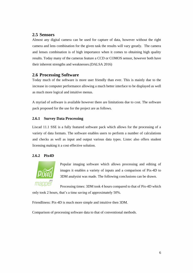
Figure 2.1 - Processing Software Accuracy

Figure 2.1 above demonstrated the similarity of both Pix4D and 3DM software

outputs(Marin Govorčin & Đapo 2014).

In conclusion Pix4D is the most efficient software for processing aerial photogrammetry

thanks to its highly developed user interface as well as efficient processing algorithms.

Pix4D has a variety of features, which include a variety of camera lens, corrections ground

point editing functions as well as many automatic systems from point cloud densification

to automatic brightness and colour correction. It has the capability of importing and

exporting over 20 data types making it a versatile tool in the surveying industry.

2.7 Limitations of Photogrammetry One of the major limitations of photogrammetry, it is limited to line of site. In terms what

the lens can see is the data that will be picked up. Hence why gaps in the data are commonly

formed. Secondly photogrammetry is limited to daytime as the requirement for

photographs with the optimal brightness is required. Also shadows and irregular shapes

can make photogrammetric readings difficult or impossible as it is a passive sensor, this in

comparison to lidar which is an active sensor. It both sends and then receives a signal.

8

2.8 Base to Height Ratio Base to height ratio greatly effects the overall quality and accuracy of a project. A study in

2000 using non digital methods found that a base to height ratio that is optimal for the

creation of a DEM is between 0.5-0.9. The question today is with current methods, is this

range still optimal and how does surveying in landscape v’s portrait effect this ratio in term

effecting the overall result of the project.

2.9 UAV Accuracy- Past Results Analysis A summary of three prior accuracy research papers are summarised below they have sole

focus of accuracy and do not relate both portrait and landscape.

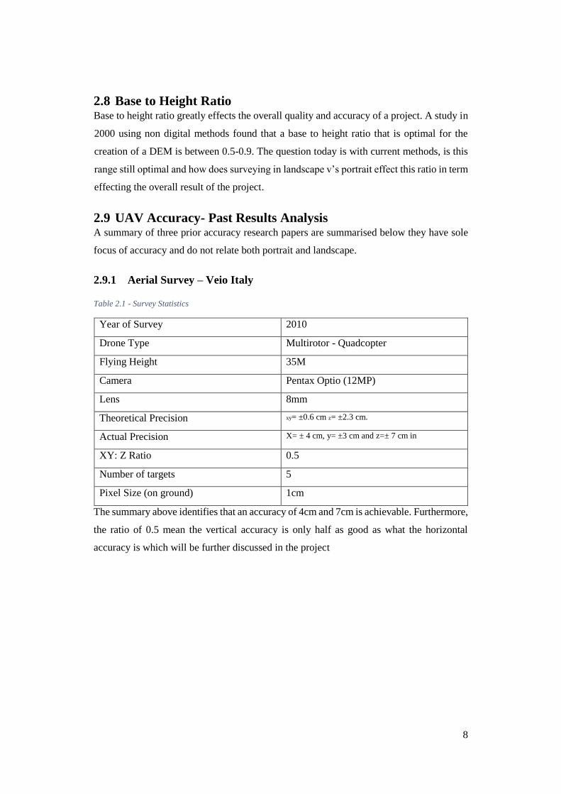
2.9.1 Aerial Survey – Veio Italy

Table 2.1 - Survey Statistics

Year of Survey 2010

Drone Type Multirotor - Quadcopter

Flying Height 35M

Camera

L

Pentax Optio (12MP)

Lens 8mm

Theoretical Precision xy= ±0.6 cm z= ±2.3 cm.

Actual Precision X= ± 4 cm, y= ±3 cm and z=± 7 cm in

XY: Z Ratio 0.5

Number of targets 5

Pixel Size (on ground) 1cm

The summary above identifies that an accuracy of 4cm and 7cm is achievable. Furthermore,

the ratio of 0.5 mean the vertical accuracy is only half as good as what the horizontal

accuracy is which will be further discussed in the project

9

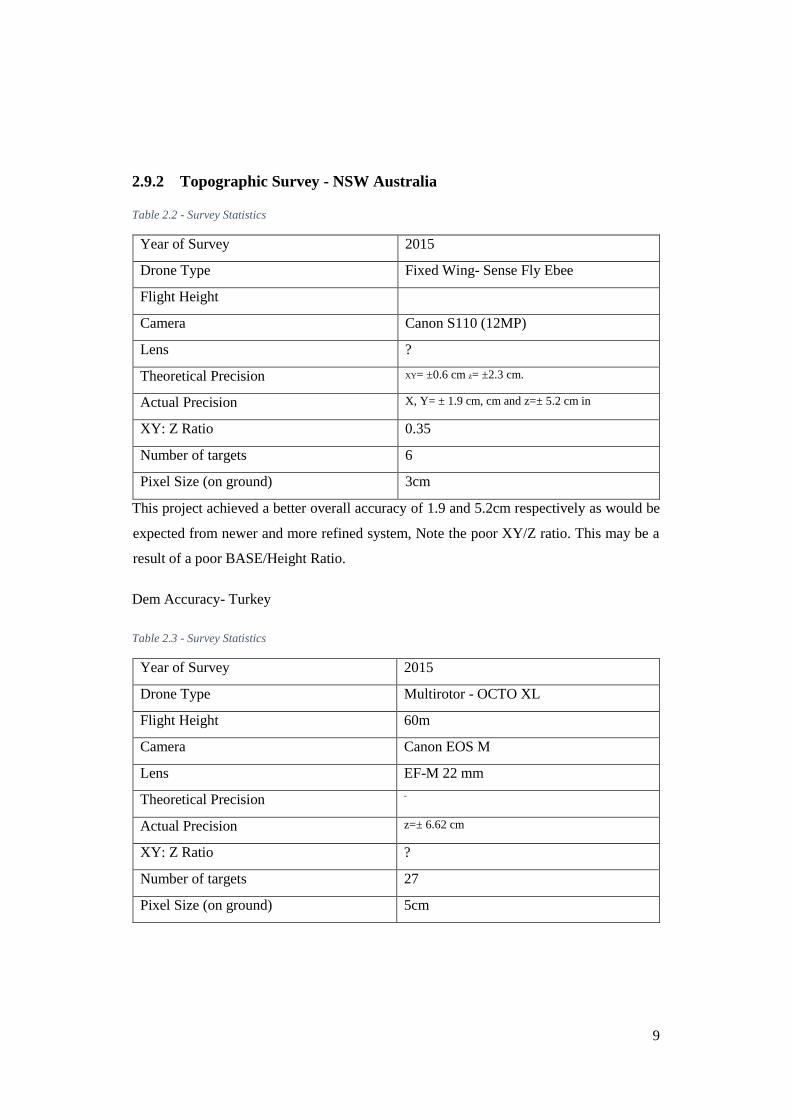
2.9.2 Topographic Survey - NSW Australia

Table 2.2 - Survey Statistics

Year of Survey

2015

Drone Type Fixed Wing- Sense Fly Ebee

Flight Height

Camera

L

Canon S110 (12MP)

Lens ?

Theoretical Precision XY= ±0.6 cm z= ±2.3 cm.

Actual Precision X, Y= ± 1.9 cm, cm and z=± 5.2 cm in

XY: Z Ratio 0.35

Number of targets 6

Pixel Size (on ground) 3cm

This project achieved a better overall accuracy of 1.9 and 5.2cm respectively as would be

expected from newer and more refined system, Note the poor XY/Z ratio. This may be a

result of a poor BASE/Height Ratio.

Dem Accuracy- Turkey

Table 2.3 - Survey Statistics

Year of Survey 2015

Drone Type Multirotor - OCTO XL

Flight Height 60m

Camera

L

Canon EOS M

Lens EF-M 22 mm

Theoretical Precision -

Actual Precision z=± 6.62 cm

XY: Z Ratio ?

Number of targets 27

Pixel Size (on ground) 5cm

10

This project utilised the highest camera specifications of all the 3 tests, however it was

flown at 60 metres (almost double the height) of the first study, however managed to

achieve a better vertical accuracy. This is likely due to the camera and lenses combination.

2.9.3 Summary

Looking at the average Z accuracy for all projects they are all similar with an average of

6.3cm in vertical accuracy. This figure will be important part of comparing and contrasting

data and results obtained in this project.

11

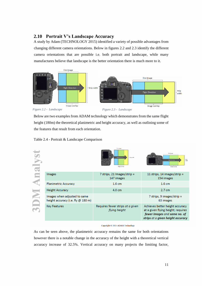
2.10 Portrait V’s Landscape Accuracy A study by Adam (TECHNOLOGY 2015) identified a variety of possible advantages from

changing different camera orientations. Below in figures 2.2 and 2.3 identify the different

camera orientations that are possible i.e. both portrait and landscape, while many

manufactures believe that landscape is the better orientation there is much more to it.

Below are two examples from ADAM technology which demonstrates from the same flight

height (180m) the theoretical planimetric and height accuracy, as well as outlining some of

the features that result from each orientation.

Table 2.4 - Portrait & Landscape Comparison

As can be seen above, the planimetric accuracy remains the same for both orientations

however there is a notable change in the accuracy of the height with a theoretical vertical

accuracy increase of 32.5%. Vertical accuracy on many projects the limiting factor,

Figure 2.2 - Landscape Figure 2.3 - Landscape

12

therefore it is highly important for further testing to be undertaken in order to identify the

real world results from the different orientations. Not only does the height accuracy

increase but there is also a reduced number of images required for a given flying height.

It important to remember that this information is from a company and not an independent

source. Also there is no direct comparison or mention of the actual results gained, these

statistics are based on calculations alone.

Some of the possible issues with portrait photogrammetry that have been discussed include;

Most platforms are not designed for portrait orientation therefore without a special

platform it may not be possible.

Overlap and sidelap must be carefully taken into consideration to ensure that

software is capable of processing the images.

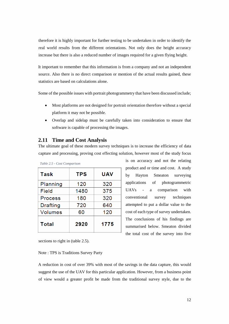
2.11 Time and Cost Analysis The ultimate goal of these modern survey techniques is to increase the efficiency of data

capture and processing, proving cost effecting solution, however most of the study focus

is on accuracy and not the relating

product and or time and cost. A study

by Hayton Smeaton surveying

applications of photogrammetric

UAVs - a comparison with

conventional survey techniques

attempted to put a dollar value to the

cost of each type of survey undertaken.

The conclusions of his findings are

summarised below. Smeaton divided

the total cost of the survey into five

sections to right in (table 2.5).

Note : TPS is Traditions Survey Party

A reduction in cost of over 39% with most of the savings in the data capture, this would

suggest the use of the UAV for this particular application. However, from a business point

of view would a greater profit be made from the traditional survey style, due to the

Table 2.5 - Cost Comparison

13

increased cost or are you likely to become non-competitive in the market particularly as

the price of drones fall while capability is enhanced.

This project did not include specific details regarding processing times as well as flight

time of UAV.

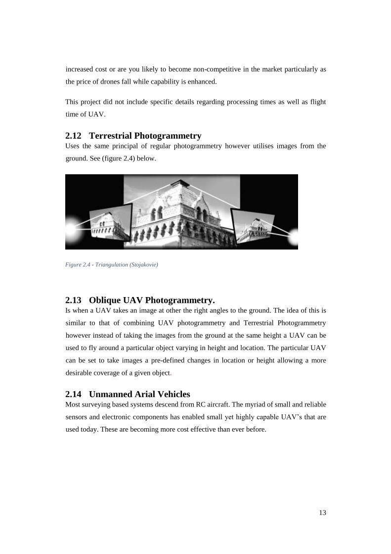
2.12 Terrestrial Photogrammetry Uses the same principal of regular photogrammetry however utilises images from the

ground. See (figure 2.4) below.

Figure 2.4 - Triangulation (Stojakovie)

2.13 Oblique UAV Photogrammetry. Is when a UAV takes an image at other the right angles to the ground. The idea of this is

similar to that of combining UAV photogrammetry and Terrestrial Photogrammetry

however instead of taking the images from the ground at the same height a UAV can be

used to fly around a particular object varying in height and location. The particular UAV

can be set to take images a pre-defined changes in location or height allowing a more

desirable coverage of a given object.

2.14 Unmanned Arial Vehicles Most surveying based systems descend from RC aircraft. The myriad of small and reliable

sensors and electronic components has enabled small yet highly capable UAV’s that are

used today. These are becoming more cost effective than ever before.

14

2.15 Types & Industry standards It is important to understand the 3 main types of UAV’s all of which require a different

type training through the CASA licensing system within Australia, for more on licensing

see section 2.3.2, The Platform types are as follows.

2.15.1.1 Fixed Wing This is the conventional plane style or delta wing type like the Ebee below.

2.15.1.2 Multirotor The most common type of UAV on the market today. The DJI phantom series is leading

the way as far as sub 2kg drones is concerned for personal use. Also compared to more

traditional fixed wing drones, multirotor UAV's have the ability to take off and land is

small spaces making them a far better solution for urban areas which are generally limited

in space.

2.15.1.3 Helicopter (rotary wing) Usually used for larger applications such as aerial spraying or high speed video recording.

System are usually very expensive.

Four systems currently used in the industry. (next page)

15

Table - 2.6 The Unmanned Arial vehicles types and specifications

Platform Ebee Trimble UX5HP Trimble ZX5 UAS Pacific CBV-

HL

Platform Type Fixed Wing Fixed Wing Multirotor Multirotor

Sensor Type and

Specifications

Photogrammetric

WX (18.2 MP)

Photogrammetric

Sony a7R 36MP

Photogrammetric

Olympus 16mp

Photogrammetric

Sony Nex-5 15MP

Sensor

Orientation

Landscape Landscape Landscape Portrait & Landscape

Flight Time 40 minutes 40 minutes 20 minutes 15 minutes

GSD 3cm 1cm 1cm 1cm

(Sensefly 2015)What accuracy and precision have other projects been able to achieve?

Industry standard Ebee RTK undertook a review to identify accuracy achieved by the

product. The following results were concluded from the assessment: The accuracy was

within 1-3 times the GSD, hence the EBEE can achieve 3cm horizontal accuracy and 5cm

vertical accuracy.

A paper by(M. Yakar 2013) conducted an experiment using 18MP cannon camera enabled

with accuracy on the 32 checkpoints ranging between 0.81cm and 8.55cm with an average

of 6.62cm.

It is evident from the research that many companies are reluctant to put actual accuracy

specifications on the systems and tend to only display this GSD of which the device is

capable. The real issue with this is that the accuracy based on the EBee GSD can vary

significantly from 1-3 times the GSD. Meaning that displaying the GSD isn’t a great

16

representation of accuracy. Not specifying accuracy helps remove the responsibility from

the company as the GSD doesn’t directly affect the accuracy instead only gives a guide to

the overall accuracy.

2.16 Licencing Within Australia to fly a drone over 2kg a licence is required for the correct type of platform

of which you are operating. However, this does not allow you to operate the aircraft.

Persons must fly under an OC (operators Certificate) again from CASA (Civil Aviation

Safety Authority) for more information and details please visit the CASA Website.

2.17 Scanning (for comparison) Scanning not dissimilar to photogrammetry however uses an active sensor. With the correct

procedure allows for the rapid capture of highly accurate spatial data for a variety of

applications from engineering to mining. Today many scanners allow for targetless from

different station setups however a paper by (Cox 2015) demonstrated issues with targetless

recognition and strongly recommended the use of targets as the use of targetless recognition

introduces unavoidable errors and misalignments to occur during the processing phase.

17

Chapter 3 - Method

3.1 Introduction This chapter identifies the proposed procedures to undertake the project in a timely and

orderly fashion. Procedures to reduce errors and reduce cost have been implemented

however due to the nature of the project the method is likely to vary, as unavoidable

obstacles are likely to occur.

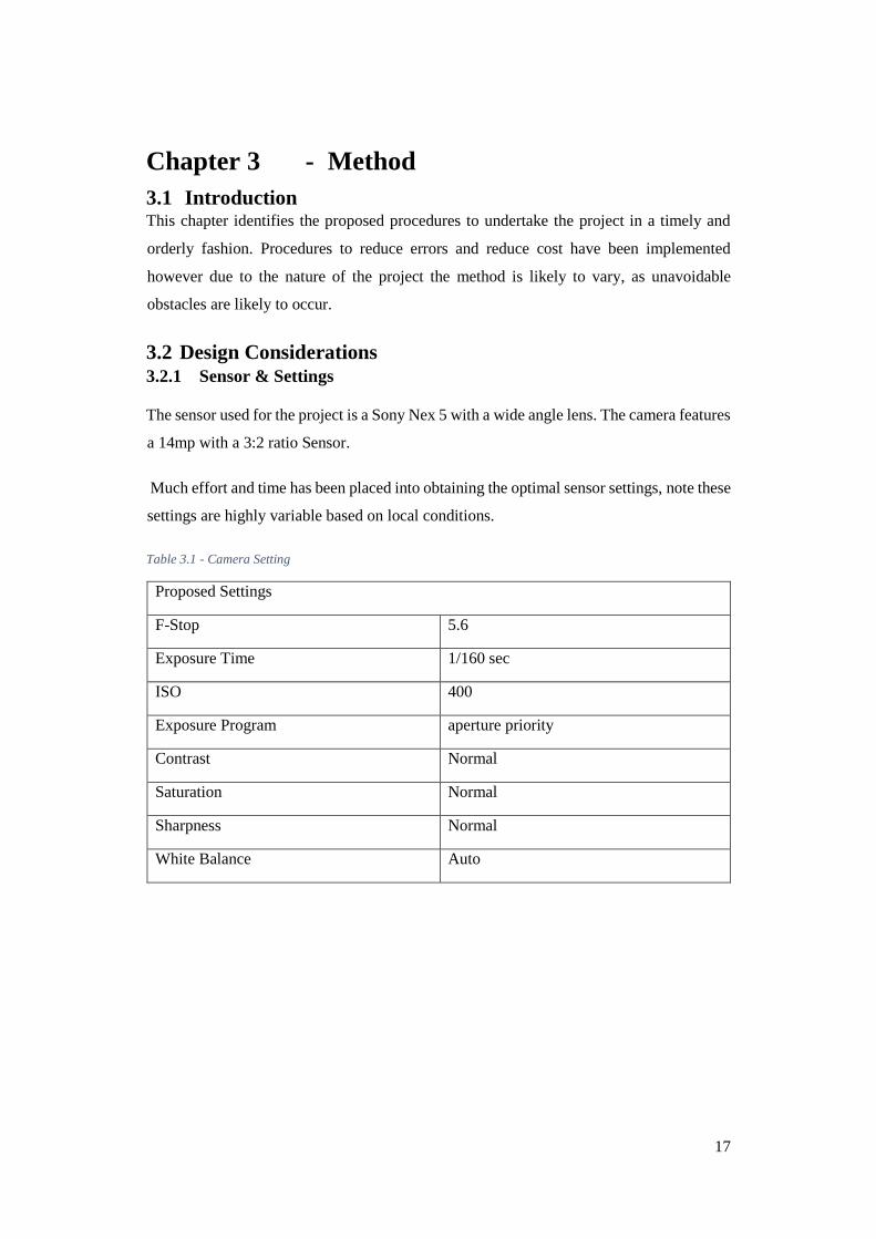
3.2 Design Considerations 3.2.1 Sensor & Settings

The sensor used for the project is a Sony Nex 5 with a wide angle lens. The camera features

a 14mp with a 3:2 ratio Sensor.

Much effort and time has been placed into obtaining the optimal sensor settings, note these

settings are highly variable based on local conditions.

Table 3.1 - Camera Setting

Proposed Settings

F-Stop 5.6

Exposure Time 1/160 sec

ISO 400

Exposure Program aperture priority

Contrast Normal

Saturation Normal

Sharpness Normal

White Balance Auto

18

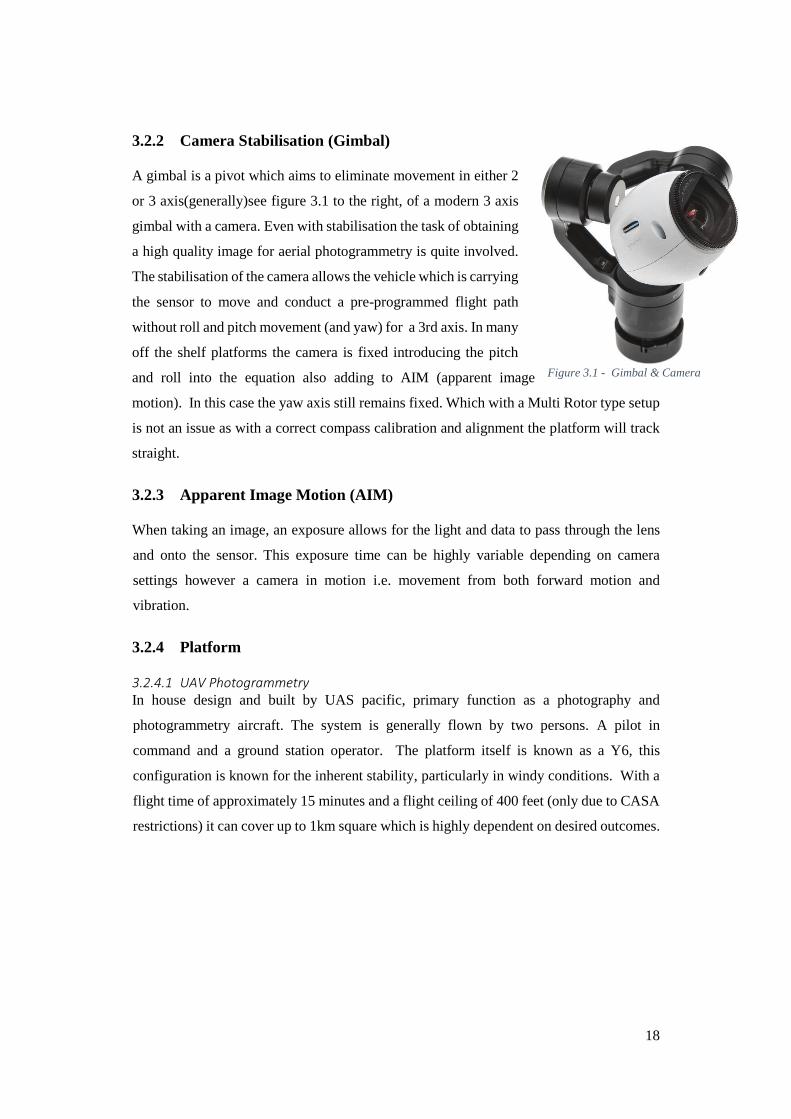
3.2.2 Camera Stabilisation (Gimbal)

A gimbal is a pivot which aims to eliminate movement in either 2

or 3 axis(generally)see figure 3.1 to the right, of a modern 3 axis

gimbal with a camera. Even with stabilisation the task of obtaining

a high quality image for aerial photogrammetry is quite involved.

The stabilisation of the camera allows the vehicle which is carrying

the sensor to move and conduct a pre-programmed flight path

without roll and pitch movement (and yaw) for a 3rd axis. In many

off the shelf platforms the camera is fixed introducing the pitch

and roll into the equation also adding to AIM (apparent image

motion). In this case the yaw axis still remains fixed. Which with a Multi Rotor type setup

is not an issue as with a correct compass calibration and alignment the platform will track

straight.

3.2.3 Apparent Image Motion (AIM)

When taking an image, an exposure allows for the light and data to pass through the lens

and onto the sensor. This exposure time can be highly variable depending on camera

settings however a camera in motion i.e. movement from both forward motion and

vibration.

3.2.4 Platform

3.2.4.1 UAV Photogrammetry In house design and built by UAS pacific, primary function as a photography and

photogrammetry aircraft. The system is generally flown by two persons. A pilot in

command and a ground station operator. The platform itself is known as a Y6, this

configuration is known for the inherent stability, particularly in windy conditions. With a

flight time of approximately 15 minutes and a flight ceiling of 400 feet (only due to CASA

restrictions) it can cover up to 1km square which is highly dependent on desired outcomes.

Figure 3.1 - Gimbal & Camera

19

3.3 Location The project focuses on accuracy particularly looking at more engineering type application

where a very high accuracy is required so to obtain the best possible best possible

comparison, the location must have the following attributes.

Areas of flat uniform land for easy comparison of surfaces.

Solid structures i.e. Buildings

Areas in the shadow of structures not seen by the photogrammetric eye in order for

terrestrial photogrammetry testing.

An area that is safe and has no restrictions in terms of the CASA regulations.

3.3.1 Control Network

Designed to optimise photogrammetry quality. To a certain point, the more control points

on a given task the higher the overall accuracy. Control must be equally spaced throughout

project. All points should be situated in a location with optimal view of the sky in hope of

points being identifiable in more images, in term increasing accuracy. The control point

accuracy will directly affect overall accuracy of the project.

3.3.2 Coordinate System

Due to the nature of the project it must only be physically correct within itself, this means

there is no requirement for a specific coordinate system to be used, instead a local

coordinate system is to be used. All photogrammetric data will be scaled and distorted

based on the data captured by the total station.

20

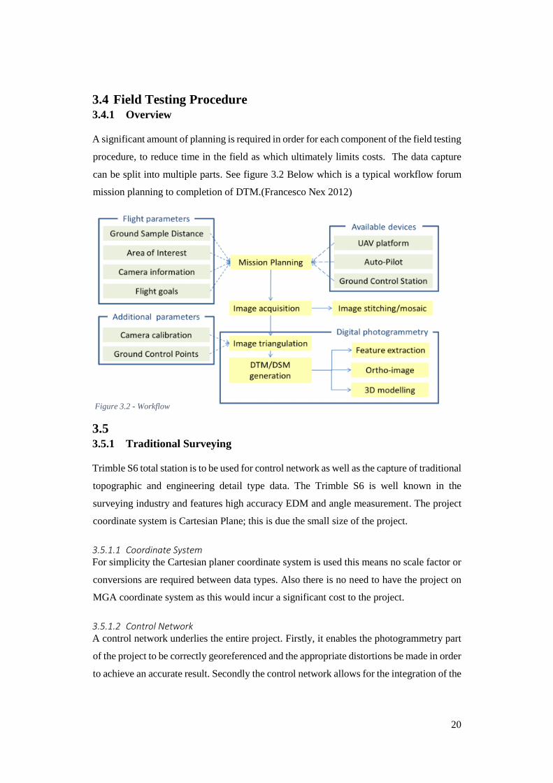
3.4 Field Testing Procedure 3.4.1 Overview

A significant amount of planning is required in order for each component of the field testing

procedure, to reduce time in the field as which ultimately limits costs. The data capture

can be split into multiple parts. See figure 3.2 Below which is a typical workflow forum

mission planning to completion of DTM.(Francesco Nex 2012)

3.5 3.5.1 Traditional Surveying

Trimble S6 total station is to be used for control network as well as the capture of traditional

topographic and engineering detail type data. The Trimble S6 is well known in the

surveying industry and features high accuracy EDM and angle measurement. The project

coordinate system is Cartesian Plane; this is due the small size of the project.

3.5.1.1 Coordinate System For simplicity the Cartesian planer coordinate system is used this means no scale factor or

conversions are required between data types. Also there is no need to have the project on

MGA coordinate system as this would incur a significant cost to the project.

3.5.1.2 Control Network A control network underlies the entire project. Firstly, it enables the photogrammetry part

of the project to be correctly georeferenced and the appropriate distortions be made in order

to achieve an accurate result. Secondly the control network allows for the integration of the

Figure 3.2 - Workflow

21

various types of data which is to be used for comparison to the photogrammetric data. This

means that the scanning data as well as the manually collected total station data can be

compared. Below is the process and quality assurance undertaken during surveying the

control network.

1. Identify suitable locations for the control network, this includes keeping control

points as evenly spaced as possible. Also care must be taken to ensure best line of

sight from the air to the ground in areas may be difficult due to vegetation.

2. Once points are identified. Using total a station take all precautions to setup

instrument and targets correctly. The network should be as ridged as possible

radiations within a control network must be avoided, each station should also have

an independent observation which may include shots from different locations.

3. Once back in the office data should be checked and processed.

3.5.1.3 Topographic data capture Known in the industry as a detail survey. In this case only small number of critical points

such as edge of road, roofs and spot heights are to be captured for data comparison.

3.5.1.4 Checks Standard surveying procedures include a variety of checks that reduce potential errors made

in the field. They include checking of backsight as well as confirming pole height and

offsets.

3.6 UAV Photogrammetry 3.6.1 Targets

A variety of targets are used in the industry however the most common are crosses and

circular type targets. Some of the circular type targets allow for further calibration within

specific software.

3.6.2 Front & Side Overlap

In order to obtain comparable results and after discussion with industry specialist, it was

decided to fly at a height of 50m with overlaps for both portrait and landscape at: Overlap

(80%) and side lap 60%. With the fixed values a true comparison between both data sets

can be made. The DJI flight planning software enables for these values to be keyed in. As

well as forwards speed (at 2m/s) Given the specified location the software calculates the

appropriate number of photographs as well as the locations of which they should be taken.

22

3.6.3 Flight Operation & Flight Path

With the on-board DJI software and ground station an area of interest for capture is

selected. The software only allows for square flight paths to be made. Furthermore, the

software allows you to define the side and forward overlap as well as flight height. Other

specifications such as sensor as well as lens specifications are also required to complete a

mission. After defining flight details the automatically generated flight path is uploaded to

the UAV. The mission can begin. Note: Prior to take off the UAV operator must have

completed the myriad of checks and appropriate paper work in order for a safe and legal

flight.

3.7 Simulations 3.7.1 Flight Time & Portrait v’s Landscape Efficiency Simulation

In order to better understand the feasibility of portrait photography. A simulations were run

to determine the time differences expected from that of both portrait and landscape as well

as comparing the number of images required to capture the given area required for survey.

Simulations are the only economical method of comparing multiple flight paths.

Simulations also reduce the risk of flying the mission.

The ground station enables a view all calculated flight details the following are of interest.

Flight Time

Number of Images

Flight Distance (total)

Shooting Distance between photographs.

3.7.1.1 Control Simulation reduces the control required as it eliminates the effect a person may

have on the outcome. i.e. Some pilots may take longer to fly a mission than other

pilots.

The simulations allow all other factors to remain fixed and the most accurate flight

time to be produced.

23

3.8 Process 1. Determine an appropriate size of survey and note its extents to apply to both

situations. Flight area of 200m*500m was selected for the simulation which is one

Hectare.

2. Based on industry knowledge apply approximate values for UAV and camera

specifications within simulations.

3. Identify the number of simulations to be made for a suitable analysis to be made.

Each flight height must have two camera orientations therefore 8 simulations are

to be made.

4. Identify the best comparison methods such as time V’s accuracy or number of

images for a given area V’s for a given accuracy.

5. Analyse results and form conclusion.

3.8.1 Processing Efficiency Simulation

The principal behind this is to identify on a per point basis if there is a benefit from

processing software on a point to time basis when processing portrait and landscape

photogrammetry. Meta data is recorded when processing is undertaking the following

information is to be collected.

Total photographs processed

Number of points created

Total processing time (for initial & rigorous)

The following steps are used and the following control measures were applied.

3.8.1.1 Control Computer specifications identical as well as temperature and weather.

No external interactions from user whilst processing in under way.

3.8.1.2 Process 1. Upload imaged and set processing going for both portrait and landscape

respectively.

2. Using the meta data as specified above.

3. Take times from flight plan used when undertaking mission.

4. Analyse using a comparison of time taken per given number of points for both the

flight time and processing time.

24

3.9 Terrestrial Photogrammetry The whole basis of using this technique is that it must be simple and efficient. It is evident

that terrestrial photogrammetry can be complete however the question is what result can

be obtained requiring a limited amount of resources and prior knowledge. So at a distance

of 5-10 metres from the chosen building taking an image every 3-4 metres with the camera

pointing directly at the target. In hope of using this additional data alongside other UAV

data collected to enhance the finished result. As far as control is concerned the idea is to

use already rectified and processed data from the air as control to tie the terrestrial

photographs. Also it is worth noting that the coordinates and orientation of the image is not

recorded in this process which may affect the outcome.

3.10 Scanning Scanning is to be used as a base for comparison, scanning with targets can provide sub

centimetre accuracy and will be a great comparison to photogrammetric data. The scanner

available for use is fairly widely used for engineering applications within Australia, the

unit is compact and is intuitive to use. As scanning is timely a small portion of this site

with the best features for comparison will be selected.

3.11 Targets To reduce errors, targets provided with the instrument are to be used. Each station is

proposed to have a minimum of 3 targets visible from station to station. The scanner is to

be set on a mid-accuracy which reduces time without compromising the quality required

for a comparison.

3.12 Data Storage To eliminate the chance of data loss, once data is captured it will be removed from mobile

device and stored on both PC and portable hard drive. Data must be easily accessible for

processing.

3.13 Processing, Comparison & Analysis 3.13.1 Data Processing

Due to the nature of the project, there is a high reliance on the use of computers and

software. A variety of software is to be used for the project and has been discussed further

in section 2.2.

It is proposed that the data processing will be completed as follows.

25

3.13.2 Preliminarily Processing

Complete initial processing of photogrammetry data to check for gaps and holes in data for

both surveying scanning and photogrammetric data. Complete further data collection if

required.

3.13.3 Traditional Surveying and Control Network Processing

Process and check control network, output in a form compatible for photogrammetry

processing. Check field work for holes. Have it prepared in Autodesk ready for data

integration.

3.13.4 Photogrammetric Processing (Pix4D)

Ultimately utilise data from section 3.12.2 and apply distortions and corrections to data.

On completion export to AutoCAD for direct comparison. However, the process is much

lengthier and can be complete using these steps below.

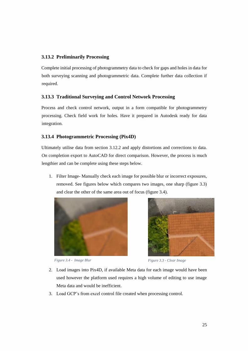
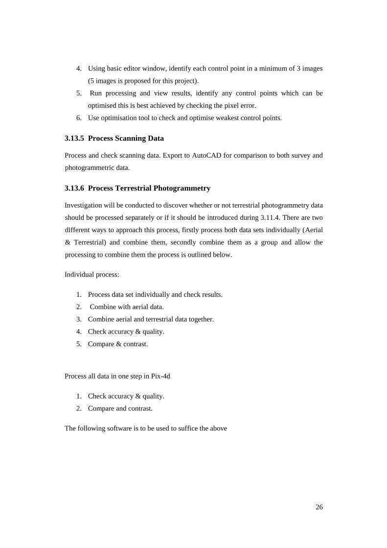
1. Filter Image- Manually check each image for possible blur or incorrect exposures,

removed. See figures below which compares two images, one sharp (figure 3.3)

and clear the other of the same area out of focus (figure 3.4).

2. Load images into Pix4D, if available Meta data for each image would have been

used however the platform used requires a high volume of editing to use image

Meta data and would be inefficient.

3. Load GCP’s from excel control file created when processing control.

Figure 3.4 - Image Blur Figure 3.3 - Clear Image

26

4. Using basic editor window, identify each control point in a minimum of 3 images

(5 images is proposed for this project).

5. Run processing and view results, identify any control points which can be

optimised this is best achieved by checking the pixel error.

6. Use optimisation tool to check and optimise weakest control points.

3.13.5 Process Scanning Data

Process and check scanning data. Export to AutoCAD for comparison to both survey and

photogrammetric data.

3.13.6 Process Terrestrial Photogrammetry

Investigation will be conducted to discover whether or not terrestrial photogrammetry data

should be processed separately or if it should be introduced during 3.11.4. There are two

different ways to approach this process, firstly process both data sets individually (Aerial

& Terrestrial) and combine them, secondly combine them as a group and allow the

processing to combine them the process is outlined below.

Individual process:

1. Process data set individually and check results.

2. Combine with aerial data.

3. Combine aerial and terrestrial data together.

4. Check accuracy & quality.

5. Compare & contrast.

Process all data in one step in Pix-4d

1. Check accuracy & quality.

2. Compare and contrast.

The following software is to be used to suffice the above

27

3.14 Photogrammetry Processing The software used for processing photogrammetry data is Pix4D. It is common in the

Survey/ UAV industry thanks to its simple yet powerful functions.

3.14.1 Scanner Processing

The scanner software is to be supplied by USQ is Faro scene. It allows the point cloud data

processed colourised from here it allows for exporting to an external software package.

Furthermore, to combine and align the data a program called mapteck i-sight studio was

used.

The laser scan data was captured using a Faro Focus 3D Laser Scanner. The data was

captured using a high resolution setting that resulted in each scan potentially capturing

approximately 176 million points.

Spherical targets were placed in the field of view for each scan. Several of these targets

were common in adjacent scans and allowed the scans to be registered, relate to each other.

This registration process was completed in the Faro Scene processing software. Each scan

was then exported in a file format compatible with the Maptek I-Site Studio program.

These exported scan files were then imported into the Maptek I-Site Studio program. The

scan data was then positioned and orientated to data captured during a total station pick-up

of the survey area. This total station pick-up was in the same relative datum as the targets

used in the UAV survey. A shed ridge line was used for this purpose, while the roof line in

the house was used to confirm the positioning of the scans. Once this process was

completed, the scan data was then re-exported through both the Maptek I-Site Studio and

Faro Scene programs in a file format that was compatible with the Liscad SEE program for

further analysis against the total station pick-up and the UAV dataset.

3.14.2 Survey, Photogrammetric and Scan Data Comparison Process

The core component of the project is the comparison on the data sets, identifying a process

which enables and un-bias analysis of the data is of utmost importance. Looking at

comparisons in the past in Smeaton and Sensefly, the comparison of only a small number

of points <100 is made the points may be randomly selected however it may not include

the entire picture missing areas which have a significant difference in terms of the overall

results. For a more thorough comparison MapteK Isight studio allows for a comparison

28

from surface to surface meaning that the entire areas chosen can be analysed comparing

hundreds of thousands of points in total allowing for a realistic comparison. A direct

comparison of scanning data to photogrammetric data was made to identify the strengths

and weaknesses of photogrammetric data. Both UAV data sets will also be compared to

further understand the limitations and accuracy of the data. Furthermore, the traditional

surveying data is primarily used as a check as well as to align and confirm the scanning

data which is to be used for the majority of the comparisons. To best analyse the data

different types of surfaces have been compared they include

Hard surfaces- (driveway) hard surface (roof).

Natural surfaces (mown grass) (high texture).

Generally, the hard surfaces are monotone type colours and have a limited amount

of texture.

Process:

Taking the data from section 3.11.4(photogrammetric data) and 3.11.5 (scanning data) the

following steps where undertaken to complete the comparison.

1) Import - all data into Maptek meaning that the scanning data, photogrammetric data as

well as the surveying data can be viewed simultaneously. Confirm scanning data

accuracy to that of the survey, shift where necessary.

2) Preparing the surfaces- A polygon was created to filter the data this mean that any data

outside the extents of the polygon will not be used in the comparison. The filter was

used to filter surfaces for comparison.

3) Tin surface and check for spiked & abnormalities which are common in scanning and

photogrammetric data.

4) Use De-Spike tools and other tool to remove noise from scanning or photogrammetric

data as required.

5) Using colour by distance from surface, select the scanning data as a base (as this is

assumed to be most correct) then select the first portrait or landscape surface as a

comparison.

6) A scale is calculated automatically and a colour grade however this can be modified as

necessary.

29

7) Before outputting select output text file, this will be used for the data analysis stage as

it includes the vertical difference in height between nearest points, hence will allow for

an in-depth analysis of an entire surface.

8) Apply the settings and view results- print screen output as required.

3.15 Data analysis Data analysis requires the use of excel and other visual as well as looking at data obtained

when processing initial photogrammetric data. The mathematical data analysis technique

discussed below was used to analyse the data.

Mean distance from the comparison surface to the model. This can be used for initial

analysis. Where individual points can be selected can compared to each other.

Process:

1. Load text file into Excel.

2. Using statistical tool bar highlight data for analysis and output statistical overview.

3. Undertake the analysis on all data sets.

4. Create appropriate charts & graphs.

30

Chapter 4 - Results

4.1 Introduction In order to form a better understanding of the project this chapter has been divided into two

main sections which consist of the results and the subsequent discussion section. This

chapter highlights the errors found in the models as well as the outcome of combining

terrestrial based photogrammetry with aerial photogrammetry.

4.2 Simulation The simulation allows an alternate view of the potential outcomes of different outcomes. It

allows the comparison of photogrammetry and different flying heights in both portrait and

landscape with minimal cost.

4.3 Accuracy Analysis Aim of this is to determine the effect of different heights on portrait v’s landscape

photogrammetry.

Firstly, the analysis identified that the planimetric accuracy remains unchanged however

there is a difference in the vertical accuracy (z axis) demonstrated below.

Table 4.1 Vertical Error, Portrait V’s Landscape

(Figure 4.1) Above shows a direct comparison between that of portrait and landscape

accuracy at a given height. Note all other variables remain fixed. An average improvement

0

0.02

0.04

0.06

0.08

120 100 80 60

Erro

r (Z

) m

etre

s

Vertical Error Portrait V's Landscape

Portrait Landscape

31

of accuracy of 33.5% is achieved when flying a mission in portrait v’s landscape based on

the above calculations. These results will be compared to actual accuracy obtained from

the field testing.

4.4 Flight Time Analysis The main question posed, is the flight time between portrait and landscape photography

significant. Also looking at the efficiency on a per point basis. The comparison determines

the number of points obtained for each second of flight. Therefore, determining the amount

of data captured for a given amount of time.

Using data obtained from processing the following can be concluded.

Total number of points collected for landscape and portrait are 26453581 and 43119418

respectively. Taking the amount of time for each flight and dividing it by the number of

seconds in each flight gives us a number of points per minute calculation. The results are

41870 V’s 45340 points a second resulting in an increase of 7.6% efficiency on a point to

time basis. Note this does not relate to the calculated increase in accuracy of each point in

the Z axis which based on the calculation exceeds 30%. This poses the question is why is

there an increase in efficiency which will be covered later in the discussion section.

4.5 Processing Time analysis 4.5.1 Processing Without Control

For initial checks and testing of data. Similar to that of section 4.4 were a number of points

per second is calculated, except this time looking at the processing time instead of the flight

time. Again the number of points obtained were the same as section 4.4 however the

processing times are significantly larger than that of the flight time of landscape and portrait

being 142 and 272 minutes respectively this gives us a per second result of 186292.8 and

158527.3 meaning that the software process the data 14% slower for portrait then that of

landscape. Again this has no relation to the actual point accuracy obtained for each point

however it identifies the point density.

4.5.2 Processing with Control

For a finished product, this relates the 3D model to the survey data. Following from section

4.5.1 the number of point as well as the related time have been recorded. Processing time

32

with control is much faster, this is probably due to many of the images already being

aligned in the ground control point adding feature.

4.6 Results - Airborne Photogrammetry Quality Report Analysis. This section covers primary project goal identifying actual accuracy’s and quality of both

portrait and landscape models.

4.6.1 Coverage Percentage

The more complete a model 3D model is in surveying in general the better the result. This

sections compares the actual point density and the coverage area obtained from each flight

of the flights undertaken.

4.6.2 Flat Surfaces

Identified as areas such as driveway and short grass.

4.6.3 Textured Surfaces

Identified as long grass, trees and roof which have an irregular formation.

4.6.4 Point Accuracy Survey Data Comparison

Compares the effect of portrait and landscape photogrammetry to that of traditional

surveying data. This comparison used the data captured from the initial survey to compare

to the photogrammetric data.

4.6.5 Point Accuracy Scanning Data Comparison

Compares the effect of portrait and landscape photogrammetry to scanning data. A total of

6 stations were used in order to capture enough data for an appropriate comparison. The

scans were uploaded into faro before being combined in Maptek eyesight studio then later

aligned to the survey data. During the pickup phase the control for the UAV was not in

place hence a number of hard services were used to align the scanning data to the survey

data. This will allow for an overall comparison between the UAV and scanning data.

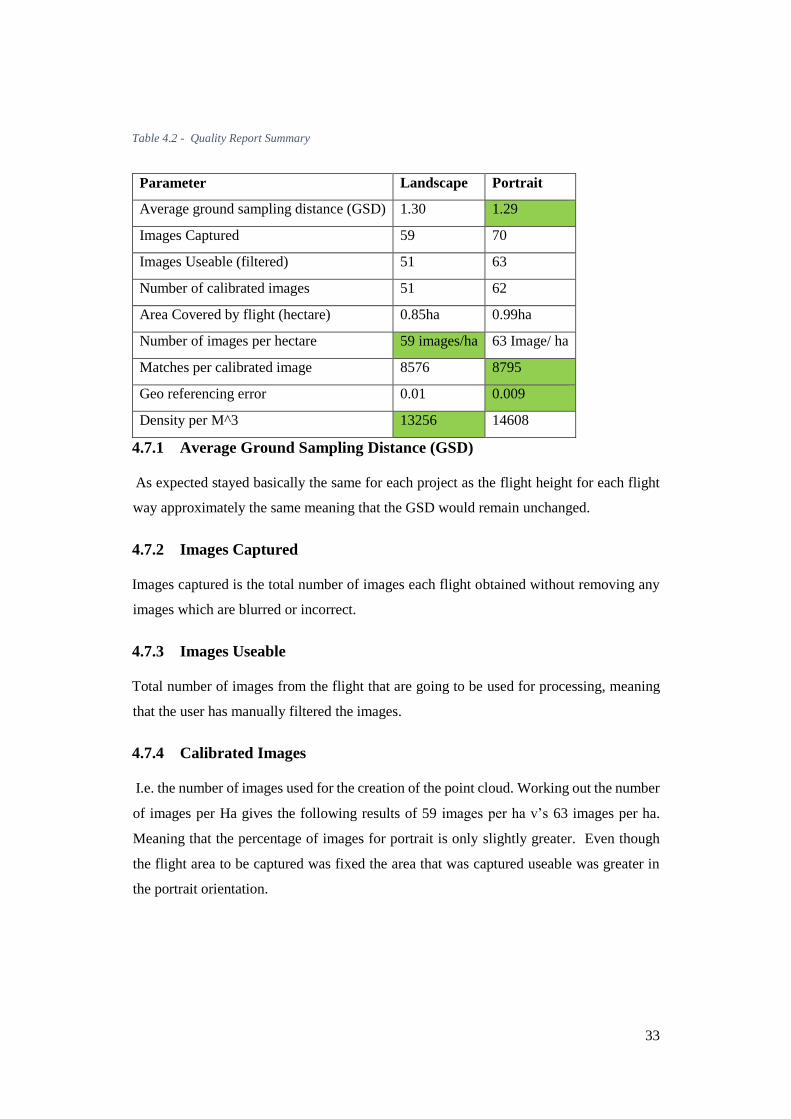
4.7 Accuracy Analysis from Quality Reports Where results can be quantified the green indicates the favourable statistic between portrait

and landscape.

33

Table 4.2 - Quality Report Summary

4.7.1 Average Ground Sampling Distance (GSD)

As expected stayed basically the same for each project as the flight height for each flight

way approximately the same meaning that the GSD would remain unchanged.

4.7.2 Images Captured

Images captured is the total number of images each flight obtained without removing any

images which are blurred or incorrect.

4.7.3 Images Useable

Total number of images from the flight that are going to be used for processing, meaning

that the user has manually filtered the images.

4.7.4 Calibrated Images

I.e. the number of images used for the creation of the point cloud. Working out the number

of images per Ha gives the following results of 59 images per ha v’s 63 images per ha.

Meaning that the percentage of images for portrait is only slightly greater. Even though

the flight area to be captured was fixed the area that was captured useable was greater in

the portrait orientation.

Parameter Landscape Portrait

Average ground sampling distance (GSD) 1.30 1.29

Images Captured 59 70

Images Useable (filtered) 51 63

Number of calibrated images 51 62

Area Covered by flight (hectare) 0.85ha 0.99ha

Number of images per hectare 59 images/ha 63 Image/ ha

Matches per calibrated image 8576 8795

Geo referencing error 0.01 0.009

Density per M^3 13256 14608

34

4.7.5 Area Covered by Flight (Hectares)

The total area of which was captured in flight based on processing. In this case the portrait

had an area 16% greater than that of landscape which is a substantial difference.

4.7.6 Number of Images Per Hectare

Calculated using the number of images used for processing and the resulting area from the

model. Portrait captures a slightly higher number of images then that of landscape meaning

an increase of 6% in the number of images required per ha verses that of landscape.

4.7.7 Number of Points Per Hectare

Takes the number of points total in the model and divide by the resultant area to give a

resulting number of points per hectare. This particular model 21853790 and 30008042 for

portrait and landscape respectively. This difference in substantial with a 27 percent increase

of points from landscape to portrait. Note this does not take into account the number

accuracy of each point gained meaning that an even larger benefit may be obtained if the

point both the number and accuracy of points increase for portrait orientation.

4.7.8 Matched Points

The number of matched point in each image will affect the quality of the calibrated images,

those areas with higher number of matching points are likely to have higher strength and

quality. In the processing above there is 3% increase in the number of matches form

landscape to that of portrait meaning that the portrait should have slightly greater strength

in terms of quality.

4.7.9 Geo-referencing Error

Is the error due to the perceived difference in location in height from different images? The

z axis on the landscape images has influenced the overall accuracy of the project with an

error or 9mm and 10mm for both portrait and landscape. In term meaning that there is little

to no difference in the fit to the control.

35

4.7.10 Image Overlap

Areas of green are likely to be of higher strength and quality. The number of overlapping

images for each flight is critical to the overall outcome, the footprint from the landscape is

more broad this is due to the greater distance between flight paths compared to that of

portrait. Meaning a higher percentage of the model may not be useable compared to the of

the portrait model again placing favour to the portrait model. Note on projects that are much

wider and require more flight paths the effect of this will be significantly reduced.

Figure 4.1 - Landscape Photo Coverage Figure 4.2 - Portrait Photo Coverage

36

4.7.11 Control Network

4.7.11.1 Network Overview Below in (figure 4.3) the layout of the control network is displayed, in this situation the

network had to be varied due to the nature of the site which has dense tree coverage in

areas.

When processing photogrammetry data the relevant software produces residuals that tell us

the potential accuracy based on the control the results are summarised below in figures 4.4

and

4

GCP X(m) Y(m) Z(m)

1 0.002 0.007 0.002

2 0.001 0.009 0.009

3 0.006 0.009 0.001

4 0.003 0.004 0.006

5 0.007 0.004 0.016

6 0.005 0.001 0.031

Mean 0.004 0.006 0.011

Standard Error 0.001 0.001 0.005

Standard Deviaiton 0.002 0.003 0.011

CI 95% 0.002 0.003 0.012

Mean Error XYZ 0.0069

Portrait

GCP X Y Z

1 0.007 0.004 0.021

2 0.007 0.002 0.021

3 0.010 0.004 0.027

4 0.005 0.004 0.002

5 0.008 0.008 0.003

6 0.004 0.006 0.001

Mean 0.007 0.005 0.013

Standard Error 0.001 0.001 0.005

Standard Deviaiton 0.002 0.002 0.012

CI 95% 0.002 0.002 0.012

Mean Error XYZ 0.008

Landscape

Figure 4.3 - Control Network

Figure 4.5 - Landscape Control Summary Figure 4.4 - Portrait Control Summary

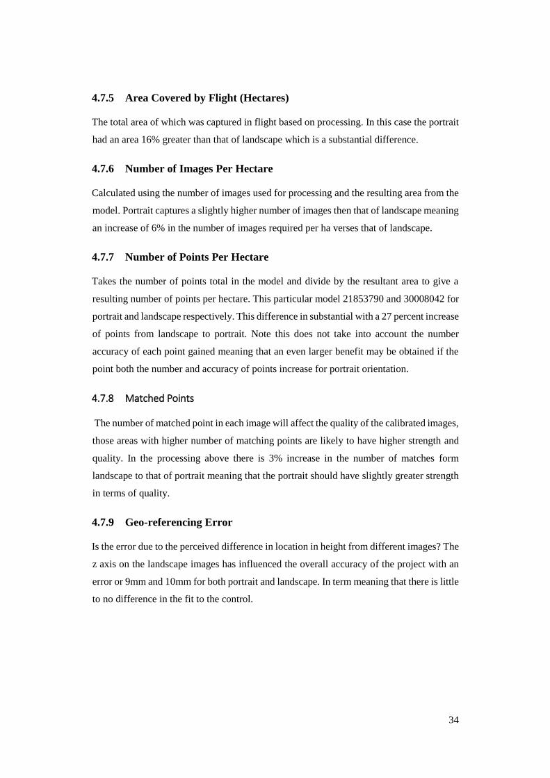
37

Firstly, from the literature (vertical) z accuracy is said to be approximately between 1-3

times the horizontal accuracy. The calculated base t height ratio is for portrait and landscape

is 1.71 and 1.44 respectively. A the slightly higher XY to Z accuracy ratio for portrait, also

saw slightly better results for both the X, and Z axis. From figure 2.1 the maximum for both

of the results is 31mm (for the z axis) furthermore there is no obvious trend in relation to

the accuracy of the control points this suggest there are no significant errors in the control

as no outliers were determined in either of the processes.

4.1 Surface Comparison The following analysis covers different surface types and their related results. The site is

split then numbered. As can been seen in Figure 4.7 and table 4.3.

Each graph has 3 different comparisons being portrait compared with the scanning data,

landscape compared with the scanning data and portrait compared with landscape

photogrammetry. Each comparison area identifies the mean, median, mode and standard

deviation.

0.000

0.002

0.004

0.006

0.008

0.010

0.012

0.014

X(m) Y(m) Z(m)

Mean Error

ERR

OR

(M)

Control Mean ErrorPortrait Landscape

Figure 4.6 - Control Error

38

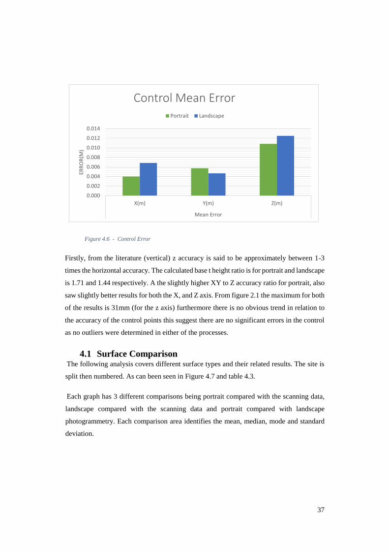
Table 4.3 - Comparison Areas Summary

Area Surface

Type/Texture

Area M^2

(Approximatly)

Points

(approximately)

1 Asphalt 60 60,0000

2 Corrugated Iron 60 60,0000

3 Grass 110 110000

4 Grass & Asphalt 80 80,0000

5 Corrugated Iron 60 60,0000

Figure 4.7 - Area Overview

39

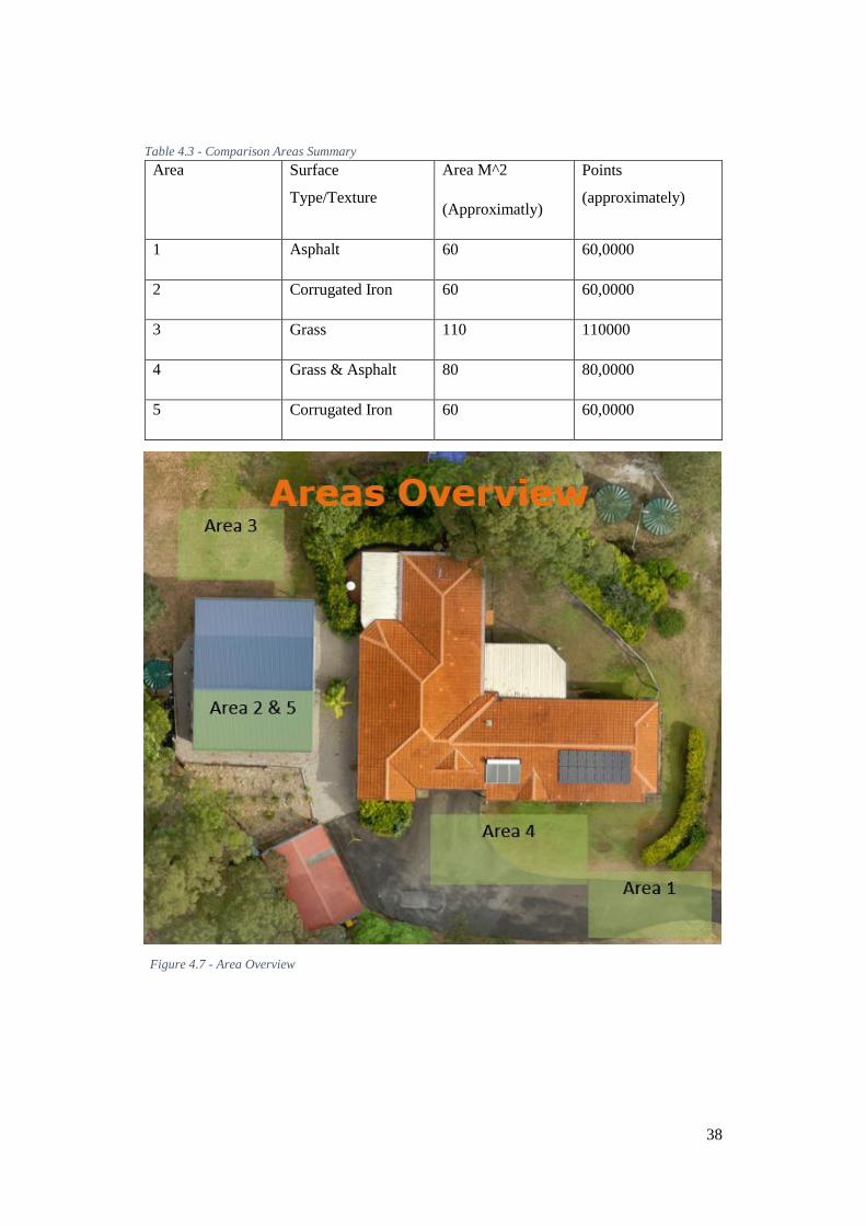
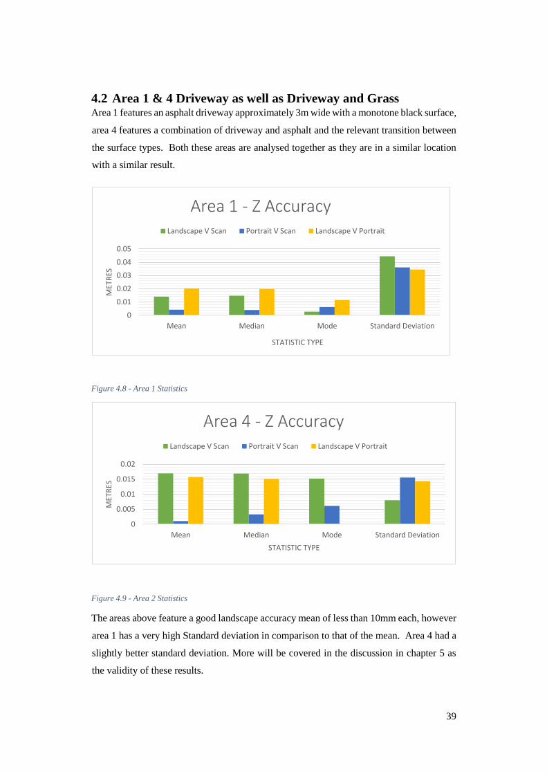
4.2 Area 1 & 4 Driveway as well as Driveway and Grass Area 1 features an asphalt driveway approximately 3m wide with a monotone black surface,

area 4 features a combination of driveway and asphalt and the relevant transition between

the surface types. Both these areas are analysed together as they are in a similar location

with a similar result.

Figure 4.8 - Area 1 Statistics

Figure 4.9 - Area 2 Statistics

The areas above feature a good landscape accuracy mean of less than 10mm each, however

area 1 has a very high Standard deviation in comparison to that of the mean. Area 4 had a

slightly better standard deviation. More will be covered in the discussion in chapter 5 as

the validity of these results.

0

0.005

0.01

0.015

0.02

Mean Median Mode Standard Deviation

MET

RES

STATISTIC TYPE

Area 4 - Z AccuracyLandscape V Scan Portrait V Scan Landscape V Portrait

0

0.01

0.02

0.03

0.04

0.05

Mean Median Mode Standard Deviation

MET

RES

STATISTIC TYPE

Area 1 - Z AccuracyLandscape V Scan Portrait V Scan Landscape V Portrait

40

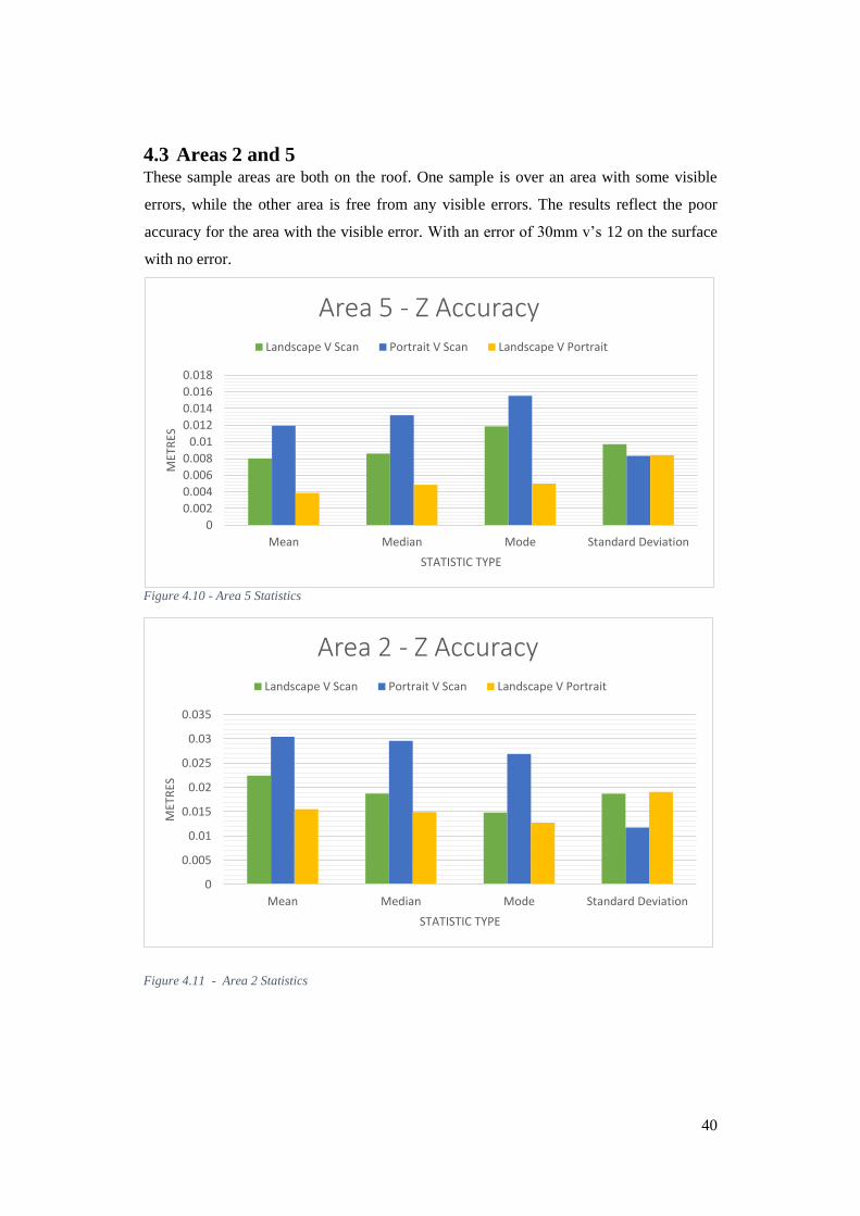
4.3 Areas 2 and 5 These sample areas are both on the roof. One sample is over an area with some visible

errors, while the other area is free from any visible errors. The results reflect the poor

accuracy for the area with the visible error. With an error of 30mm v’s 12 on the surface

with no error.

Figure 4.10 - Area 5 Statistics

Figure 4.11 - Area 2 Statistics

0

0.005

0.01

0.015

0.02

0.025

0.03

0.035

Mean Median Mode Standard Deviation

MET

RES

STATISTIC TYPE

Area 2 - Z AccuracyLandscape V Scan Portrait V Scan Landscape V Portrait

0

0.002

0.004

0.006

0.008

0.01

0.012

0.014

0.016

0.018

Mean Median Mode Standard Deviation

MET

RES

STATISTIC TYPE

Area 5 - Z AccuracyLandscape V Scan Portrait V Scan Landscape V Portrait

41

4.4 Area 3 Short Grass This area has a high texture. The ground itself sloping however makes a good comparison

for natural surface type areas. In this area the standard devation is one of the lowest of all

the areas even though it has one of the highest means.

Figure 4.12 - Area 3 Statistics

4.5 Surfaces Summary In summary the mean of all the results can be seen below. The mean over the entire surface

was similar for both portrait and landscape.

Figure 4.13 - Combined Area Statistics

0

0.01

0.02

0.03

0.04

0.05

Mean Median Mode Standard Deviation

MET

RES

STATISTIC TYPE

Area 3 - Z AccuracyLandscape V Scan Portrait V Scan Landscape V Portrait

0

0.005

0.01

0.015

0.02

0.025

Mean Median Mode Standard Deviation

MET

RES

STATISTIC TYPE

All Areas - Z Accuracy

Landscape V Scan Portrait V Scan Landscape V Portrait

42

4.6 Results Ground Based Photogrammetry The attempt to try and easily combine terrestrial photogrammetry with aerial

photogrammetry has not been successful in this particular case. There are several reasons

I believe it was not a success. Firstly, trying to combine a large of number of images without

any geolocation spread over a site was not going to work unless the software identified

where each image was from. The biggest issues with this was that the images could not

relate to other images as they were taken at right angles and did not include enough of the

same data in order to match the aerial and terrestrial images.

The first attempt at combining the images as described in method one resulted with none

of the terrestrial images being used for the model. This was a surprise as PIX4D is definitely

capable however the capture method must not have been desirable in terms of overlap.

Using method two the images where processed individual as an entire group with only a

very small portion of images being recognised. A final attempt was made to combine the

images as induvial sets for each object. However, this still had only very limited success.

The question in why didn’t it work and how could we get it to work.

Potential Issues

Image overlap

Geo location

Control

This raises the question is it likely that the requirements for planning, the use of control as

well as the processing time a practical option for surveyors.

It also raises the question would units such as the V10 be a cost effective solution to

reducing the number of gaps from airborne photogrammetric data.

43

Chapter 5 - Discussion

5.1 Introduction This section covers further information regarding portrait and landscape photogrammetry.

Looking at the number of landscape orientated platforms.

5.1.1 Area 1 & 4 –Discussion

Saw the lowest mean distance from surface to surface however, achieved a poor standard

deviation exceeding 40mm the cause of this error is shadows which is covered in section

5.1.5. the area not effected by shadows have a significantly better standard deviation. When

landscape the surface is compared to the portrait surface the errors mean is less than 5mm.

5.1.2 Areas 2 and 5 Discussion

Area two has visible errors in the model however both portrait and landscape both achieved

accuracy of less than 30mm. The surface 5 which does not include the error is still

noticeably worse accuracy then that of area 1 and 4. This raises the question why is the

accuracy worse and how can we improve the accuracy on the building. In the case of this

unless the GSD is small enough to capture the actual undulations in the corrugation a false

flat surface is represented (which is the case here) whereas the scanner itself picks up actual

points, meaning that the scanning surface may have an approximate flat surface with

undulations. Hence causing a higher mean distance from surface to surface compared to

the road. Also effecting the results is the change in height as well as not using any control

on the building itself. The use of targets or locating some of the corners in the model and

using this to process would greatly increase the accuracy. (Sauerbier).

5.1.3 Area 3 –Discussion

The grass in this area is much thinner than that of area 1, even though the grass is short it

long enough to affect the results. Portrait was higher as suspected from photogrammetry.

However, the landscape surface was lower than that of the scan. It’s worth note that the

land is on a slight slope. However, I don’t think this would have significant effect on the

project.

44

5.1.4 Surfaces Summary Discussion

Looking at all the results as a whole, the overall accuracy in terms of z is surprisingly good

with both portrait and landscape being less than 16mm with portrait slightly better than that

of landscape.

5.1.5 Shadows

As mentioned in the results, area 1 whilst overall had a great mean surface, however in

relation to the range and standard deviation the results were poor meaning that many of the

results were outside of 30mm some exceeding 100mm. A paper by M. Sauerbie in 2005

suggest the largest errors occur on steep surfaces with a low texture not a flat surface (like

a road). After analysing the images and some research on the internet the most likely of the

error is shadow. The accuracy standard deviation of the surface with the shadows (area 1)

was approximately 40mm compared to area 4 which should have had a similar result was

less than half of that of area 1 (15mm), meaning that the quality of the data is highly

compromised when shadows are present. Trees are present on many country and a suburban

roads meaning caution should be taken in order to prevent errors. See figures 5.1 & 5.7,

firstly an overview of the shadows (Arial image) secondly a view of the model which has

a visual error on the area where the shadow is. To reduce these errors effort should be made

to pick flight times with minimal shadows and or overcast conditions which greatly reduce

the shadows.

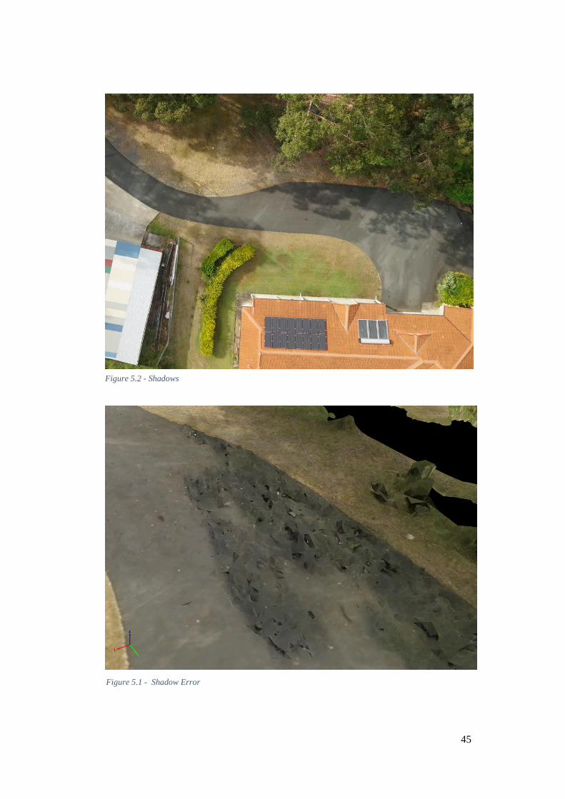
45

Figure 5.1 - Shadow Error

Figure 5.2 - Shadows

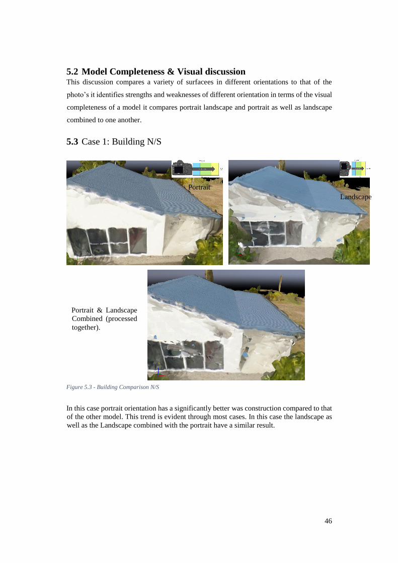
46

5.2 Model Completeness & Visual discussion This discussion compares a variety of surfacees in different orientations to that of the

photo’s it identifies strengths and weaknesses of different orientation in terms of the visual

completeness of a model it compares portrait landscape and portrait as well as landscape

combined to one another.

5.3 Case 1: Building N/S

In this case portrait orientation has a significantly better was construction compared to that

of the other model. This trend is evident through most cases. In this case the landscape as

well as the Landscape combined with the portrait have a similar result.

Figure 5.3 - Building Comparison N/S

Portrait

Landscape

Portrait & Landscape

Combined (processed

together).

47

5.4 Case 2 : NE Building

This case clearly shows the difference between portrait and landscape. The building itself

has a far better appearance and structure then that of the landscape. The portrait and

landscape model has an appearance quality between that of portrait and landscape. This

case again demonstrates a better clarity and formation on the image/model for the portrait

model (top left) however this is less significant in this particular model. Note that the

portrait and landscape combined model appears to be in-between the quality of that of the

portrait and landscape models.

Figure 5.4 - Building Comparison N/E

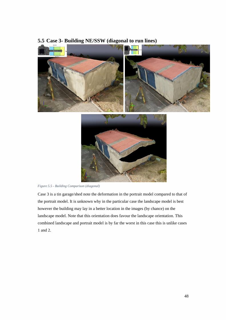
48

5.5 Case 3- Building NE/SSW (diagonal to run lines)

Case 3 is a tin garage/shed note the deformation in the portrait model compared to that of

the portrait model. It is unknown why in the particular case the landscape model is best

however the building may lay in a better location in the images (by chance) on the

landscape model. Note that this orientation does favour the landscape orientation. This

combined landscape and portrait model is by far the worst in this case this is unlike cases

1 and 2.

Figure 5.5 - Building Comparison (diagonal)

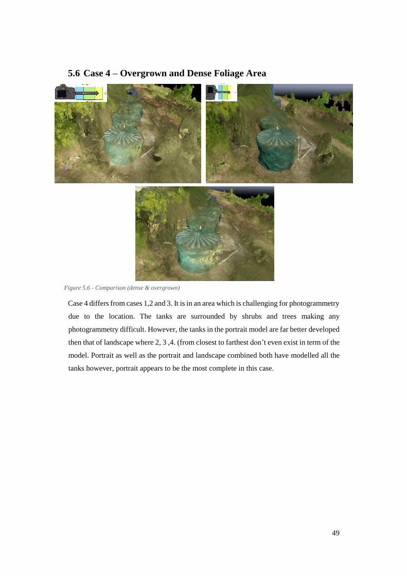
49

5.6 Case 4 – Overgrown and Dense Foliage Area

Case 4 differs from cases 1,2 and 3. It is in an area which is challenging for photogrammetry

due to the location. The tanks are surrounded by shrubs and trees making any

photogrammetry difficult. However, the tanks in the portrait model are far better developed

then that of landscape where 2, 3 ,4. (from closest to farthest don’t even exist in term of the

model. Portrait as well as the portrait and landscape combined both have modelled all the

tanks however, portrait appears to be the most complete in this case.

Figure 5.6 - Comparison (dense & overgrown)

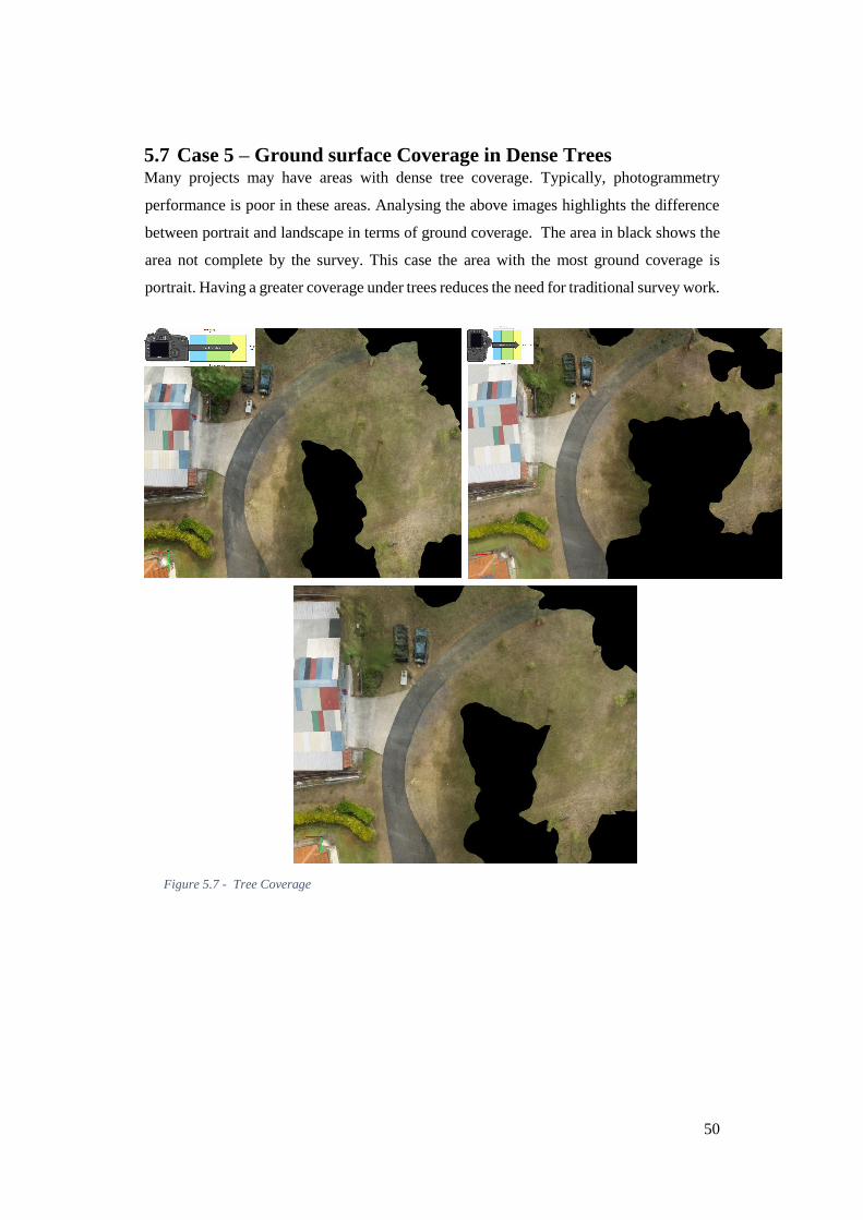
50

5.7 Case 5 – Ground surface Coverage in Dense Trees Many projects may have areas with dense tree coverage. Typically, photogrammetry

performance is poor in these areas. Analysing the above images highlights the difference

between portrait and landscape in terms of ground coverage. The area in black shows the

area not complete by the survey. This case the area with the most ground coverage is

portrait. Having a greater coverage under trees reduces the need for traditional survey work.

Figure 5.7 - Tree Coverage

51

5.8 Model Completeness & visual discussion conclusion From analysing a series of cases comparing the 3 models in the 5 cases it can be concluded

that portrait has definite advantage being better in 4 out of the 5 comparisons. Furthermore,

the following statements have been derived.

Portrait camera orientation produces better modelling (visually) of building and

structures.

Structures close two or near obstacles are generally better formed in portrait

photogrammetry.

Greater coverage of ground, in areas under trees is achieved by portrait

photogrammetry.

5.8.1 Summary Table

Table 5.1 - Comparison Summary

5.8.2 Why does Portrait Capture Some Areas Otherwise Missed by

Landscape?

Below figures 5.8 and 5.9 show the difference between the photo station layout for portrait

(at top) and landscape down the bottom. Overall the spacing for the images is better for

portrait hence allowing for a greater number of points as well as capturing data in more

marginal areas.

Orientation Portrait Landscape Portrait &

Landscape

Case 1 -Building Best Poor Better

Case 2 - Building Best Poor Better

Case 3 - Building Better Best Poor

Case 4 – Structure

Difficult location

Best Poor Better

Case 5 – Ground coverage

(under Trees)

Best Poor Better

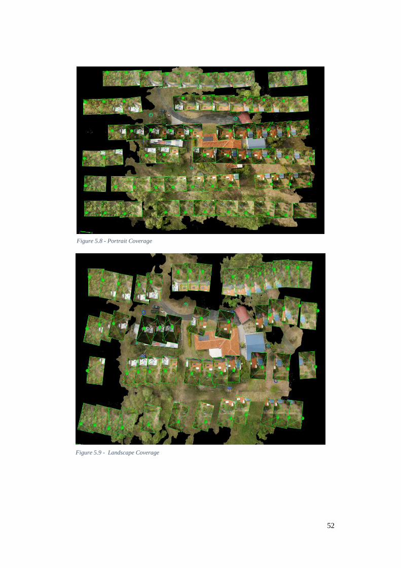
52

Figure 5.8 - Portrait Coverage

Figure 5.9 - Landscape Coverage

53

5.8.3 Camera Orientation Practicality

Why do some manufactures (particularly multirotor) not have the ability to change the

camera orientation? First let’s look at multirotor platforms.

5.8.3.1 Multirotor Physical Limitations - Many of the low end systems (phantom) have a fixed camera

direction meaning that the orientation cannot be changed (without advanced technical

knowledge). Many larger systems also have only a two axis gimbal, meaning that the

gimbal would physically have to be turned 90 degrees in order to achieve portrait

orientation. The best option for this application (change between portrait and landscape)

is the use of a 3 axis gimbal that can be programmed to face in both orientations with

options for both built into the software. Then depending on the job an orientation can be

selected.

Centre of Gravity - The cameras are hung from a gimbal (which must be balanced)

assuming no changes in the balance and location of the gimbal the COG will not be

changed.

Software - In terms of flight planning many of the main stream planners do not allow the

change of parameters which would allow for changing camera orientation.

5.8.3.2 Fixed Wing Physical Limitations - Many of the fixed wing platforms on the market are highly compact

and therefore are not designed to allow for different camera orientations. Fixed wings

generally have internally mounted cameras and do not have a gimbal, meaning that the

camera is moved along with the airframe which in turbulent conditions may have a

detrimental effect on the results.

Centre of Gravity - Due to the nature of the shelf platforms they often only have a small

envelope of which the COG must be within. Particularly with flying wings. Therefore,

platforms engineered for cameras in a certain orientation must remain in that orientation to

make sure the COG remains within manufacturer specification.

Software - Most off the shelf systems software does not include flight planning for cameras

in alternate orientations.

54

Chapter 6 - Conclusion

6.1.1 Findings

The height accuracy of portrait v’s landscape photogrammetry was not found to be

significant. Furthermore, an increase in number of images and runs (potentially) for the

same area coverage does not make portrait photogrammetry economical. The accuracy

difference may not have been significant however, structures in areas with dense trees had

a noticeable advantage. In some cases, structures that were not formed with landscape were

completely formed with portrait, furthermore portrait allows a larger area under the canopy

to be mapped in comparison to that of landscape. Furthermore, this project highlights the

effect of environmental conditions on the overall results of the project. In particular, the

effect of shadows (which appears to be heightened on low texture surfaces) such as a road.

It is recommended that flights where heights are critical that they are flown at times with

the lowest shadow footprint (around midday) or even better in light overcast conditions

which act as a filter and greatly reduce if not eliminate shadows.

6.1.2 Testing Limitations

Financial constraints

Due to the nature of the project and having to use UAV’s, the amount of testing was limited

to only one site and two different flights and flight parameters. This ultimately means that

there is the potential for more comparisons of data sets with varying base to height ratios

as well as side lap. Furthermore, only a single software package was used for the

processing. Results may vary significantly with the use of other processing software.

Unknown errors

Only errors that were known about were analysed. The potential for other errors that have

not been covered may have affected the outcome.

55

6.2 Further Research The following areas have the potential for further works, they include.

(Research 1) Terrestrial & Airborne photogrammetry combination

(Research 2) Airborne oblique photogrammetry with normal airborne

photogrammetry.

(Research 3) Multi Sensor combination.

6.2.1 Research 1

This area has the potential to reduce the so called gaps in the data, taking what I have learnt

from my project as well as other relevant projects completed this year (2016) the

combination of data sets may allow for a greatly reduced amount of field work required by

surveyors. Pix-4D is becoming increasingly advanced and allows the user to process

project both individually and separately.

6.2.2 Research 2

Similar to that of Research 1 however uses a UAV to capture the oblique images. The idea

again reducing the gaps in the data. This raises the question can normal aerial

photogrammetry be processed, from here the areas in the capture that are missed which are

still required. Could they automatically be included in a flight path which identifies

possible safe flight paths (missing obstacles mapped) to then semi- automatically capture

the data required to fill in the gaps.

6.2.3 Research 3

An area relatively untouched, it looks at the combination of sensor types. For instance, the

use of photogrammetry alongside scanning. The idea being that the weaknesses in the

different sensor types are eliminated. Take the area of focus in my project (country housing

lot) where there are a variety of structure types as well as vegetation coverage. The aim

being to capture not only the trees but the natural surface below. As well as more accurate

information on the fixed surface. Then with use of a lidar type system to capture the areas

in shadow from trees and in shadow. Then combine this with photogrammetry data. Some

of the main factors which are likely to influence the cost is the significant cost of utilising

these sensors, furthermore finding a platform (UAV) which is capable of carrying both the

56

sensors. Other challenges may include the processing and combining of data. As smaller

sensors are developed its more likely to become feasible!

57

Bibliography

Colomina, l 2014, 'ISPRS Journal for photogrammetry & remote sensing ', Unmanned

aerial systems for photogrammetry and remote sensing: A review, pp. 79-97,

<http://www.sciencedirect.com/science/article/pii/S0924271614000501>

Cox, R 2015, 'Real-world comparisons between target-based

and targetless point-cloud registration in FARO

Scene, Trimble RealWorks and Autodesk Recap', University of Southern Queensland.

DALSA, T 2016, CCD vs. CMOS, https://www.teledynedalsa.com/imaging/knowledge-

center/appnotes/ccd-vs-cmos/>

F. Remondino a, LBbFNa, M. Scaioni b , D. Sarazzi c 2011, International Archives of the

Photogrammetry, Remote Sensing and Spatial Information Sciences, Vol. XXXVIII-1/C22

UAV-g 2011, Conference on Unmanned Aerial Vehicle in Geomatics, Zurich, Switzerland

viewed 18/08/2016, <http://www.geometh.ethz.ch/uav_g/proceedings/remondino>

Francesco Nex, FR 2012, 'UAV for 3D mapping applications', viewed 2016,

<http://3dom.fbk.eu/sites/3dom.fbk.eu/files/pdf/Nex_Remondino_AG2013_pre-

print.pdf>

M. Yakar, MU, A.S. Toprak, N.Polat 2013, '3D MODELING OF HISTORICAL DOGER

CARAVANSARIES BY DIGITAL

PHOTOGRAMMETRY', in Proceedings of XXIV International CIPA Symposium,

Strasbourg, France, http://www.int-arch-photogramm-remote-sens-spatial-inf-sci.net/XL-

5-W2/695/2013/isprsarchives-XL-5-W2-695-2013.pdf>.

Marin Govorčin, migeg, Prof. Dr. Boško Pribičević, Assist. Prof. & Đapo, DA 2014,

'COMPARISON AND ANALYSIS OF SOFTWARE SOLUTIONS FOR

CREATION OF A DIGITAL TERRAIN MODEL USING UNMANNED AERIAL

VEHICLES',

<https://www.researchgate.net/profile/Marin_Govorcin/publication/263548181_COMPA

RISON_AND_ANALYSIS_OF_SOFTWARE_SOLUTIONS_FOR_CREATION_OF_A

_DIGITAL_TERRAIN_MODEL_USING_UNMANNED_AERIAL_VEHICLES>

58

Sauerbier, M 'ACCURACY OF AUTOMATED AEROTRIANGULATION AN', viewed

5/62016, <http://e-collection.library.ethz.ch/eserv/eth:28023/eth-28023-01.pdf>

Schenk, T 1996, 'Digital Aerial Triangulation', Ohio State University.

Sensefly 2015, 'Ebee RTK Assessment', p. 7, viewed 27/10/2015,

<https://www.sensefly.com/fileadmin/user_upload/sensefly/documents/eBee-RTK-

Accuracy-Assessment.pdf>

Stojaković, V 2008, 'TERRESTRIAL PHOTOGRAMMETRY AND APPLICATION TO

MODELING ARCHITECTURAL OBJECTS '.

TECHNOLOGY, A 2015, 'Processing UAV Projects', viewed 20/10/15,

<http://www.adamtech.com.au>

59

Appendix A

Project Specification

For: Bradley Redding

Title: 3D modelling for surveying projects using Unmanned Arial

Vehicles (UAVs) and Laser scanning.

Major: Surveying

Supervisors: Zahra Gharineiat

Enrolment: ENG4111 – EXT S1, 2016

ENG4112 – ONC S2, 2016

Project Aim: Determine the effect of portrait & landscape photogrammetry on

overall accuracy of the resulting model as well as investigate the use of terrestrial

photogrammetry alongside airborne photogrammetry in order to create a more complete

3D model hence a better product.

Programme: Issue B, 4th march 2016

1. Identify/ research appropriate specifications for data capture.

2. Create a plan to capture data as well as identify instruments required.

3. Process data using appropriate software.

4. Analyse and compare models and identify if changes need to be made to the

model in order to improve the overall results.

5. Capture more data as required to enhanced the model.

6. Make recommendations as to the use of portrait v’s landscape photogrammetry.

As well as the use of terrestrial photogrammetry and if it is an effective method

of capture for industry.

If time permits:

7. Present findings and results to a conference and obtain feedback from the public.

Quality Report

60

Appendix B

Generated with Pro version 2.2.22

Important: Click on the different icons for:

Help to analyze the results in the Quality Report

Additional information about the sections

Click here for additional tips to analyze the Quality Report

Summary

Project project test #5 landscape 2.2

Processed 2016-08-17 06:12:56

Camera Model Name(s) NEX-5N_E18-55mmF3.5-

5.6OSS_19.0_4912x3264 (RGB)

Average Ground Sampling

Distance (GSD)

1.3 cm / 0.51 in

Area Covered 0.014 km2 / 1.3983 ha / 0.0054 sq. mi. / 3.4571

acres

Time for Initial Processing

(without report)

08m:05s

Quality Check

Images median of 51723 keypoints per image

Dataset 51 out of 51 images calibrated (100%), all images enabled

Camera

Optimization

2.5% relative difference between initial and optimized internal

camera parameters

Matching median of 7047.43 matches per calibrated image

Georeferencing yes, 6 GCPs (6 3D), mean RMS error = 0.009 m

Preview

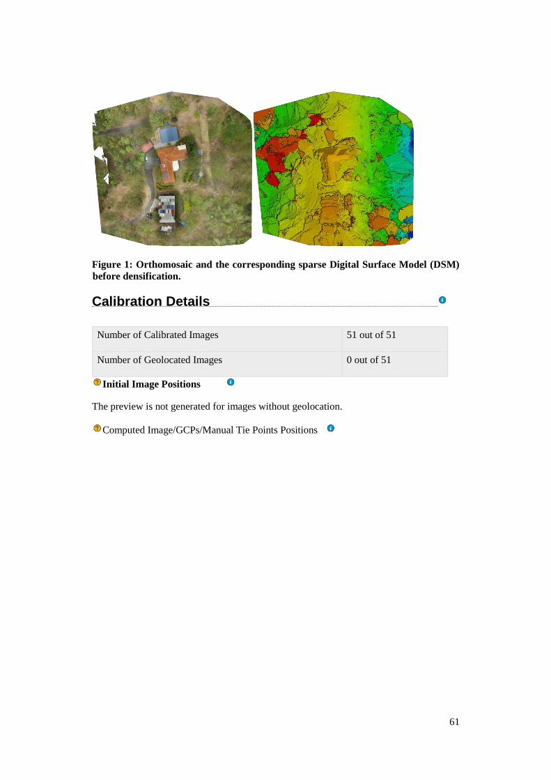
61

Figure 1: Orthomosaic and the corresponding sparse Digital Surface Model (DSM)

before densification.

Number of Calibrated Images 51 out of 51

Number of Geolocated Images 0 out of 51

Initial Image Positions

The preview is not generated for images without geolocation.

Computed Image/GCPs/Manual Tie Points Positions

Calibration Details

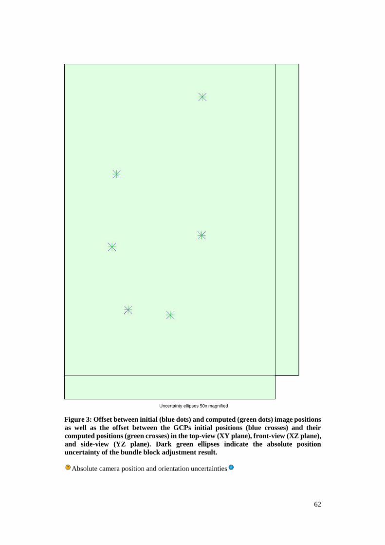
62

Figure 3: Offset between initial (blue dots) and computed (green dots) image positions

as well as the offset between the GCPs initial positions (blue crosses) and their

computed positions (green crosses) in the top-view (XY plane), front-view (XZ plane),

and side-view (YZ plane). Dark green ellipses indicate the absolute position

uncertainty of the bundle block adjustment result.

Absolute camera position and orientation uncertainties

Uncertainty ellipses 50x magnified

63

X

[m]

Y

[m]

Z [m] Omega [degree] Phi [degree] Kappa [degree]

Mean 0.039 0.041 0.129 0.045 0.043 0.011

Sigma 0.006 0.013 0.005 0.014 0.008 0.004

Overlap

Figure 4: Number of overlapping images computed for each pixel of the orthomosaic.

Red and yellow areas indicate low overlap for which poor results may be generated.

Green areas indicate an overlap of over 5 images for every pixel. Good quality results

will be generated as long as the number of keypoint matches is also sufficient for these

areas (see Figure 5 for keypoint matches).

Number of 2D Keypoint Observations for Bundle Block Adjustment 384125

Number of 3D Points for Bundle Block Adjustment 148373

Mean Reprojection Error [pixels] 0.159

Number of overlapping images: 1 2 3 4 5+

Bundle Block Adjustment Details

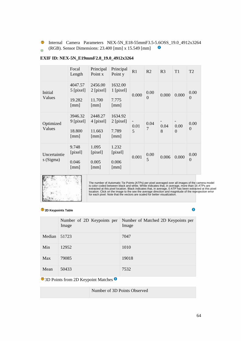
64

Internal Camera Parameters NEX-5N_E18-55mmF3.5-5.6OSS_19.0_4912x3264

(RGB). Sensor Dimensions: 23.400 [mm] x 15.549 [mm]

EXIF ID: NEX-5N_E19mmF2.8_19.0_4912x3264

Focal

Length

Principal

Point x

Principal

Point y R1 R2 R3 T1 T2

Initial

Values

4047.57

5 [pixel]

19.282

[mm]

2456.00

2 [pixel]

11.700

[mm]

1632.00

1 [pixel]

7.775

[mm]

0.000 0.00

0 0.000 0.000

0.00

0

Optimized

Values

3946.32

9 [pixel]

18.800

[mm]

2448.27

4 [pixel]

11.663

[mm]

1634.92

2 [pixel]

7.789

[mm]

-

0.01

5

0.04

7

-

0.04

8

-

0.00

0

0.00

0

Uncertaintie

s (Sigma)

9.748

[pixel]

0.046

[mm]

1.095

[pixel]

0.005

[mm]

1.232

[pixel]

0.006

[mm]

0.001 0.00

5 0.006 0.000

0.00

0

Number of 2D Keypoints per

Image

Number of Matched 2D Keypoints per

Image

Median 51723 7047

Min 12952 1010

Max 79085 19018

Mean 50433 7532

3D Points from 2D Keypoint Matches

Number of 3D Points Observed

The number of Automatic Tie Points (ATPs) per pixel averaged over all images of the camera model is color coded between black and white. White indicates that, in average, more than 16 ATPs are extracted at this pixel location. Black indicates that, in average, 0 ATP has been extracted at this pixel location. Click on the image to the see the average direction and magnitude of the reprojection error for each pixel. Note that the vectors are scaled for better visualization.

2 D Keypoints Table

65

In 2 Images 105890

In 3 Images 23419

In 4 Images 8715

In 5 Images 4286

In 6 Images 2346

In 7 Images 1324

In 8 Images 901

In 9 Images 590

In 10 Images 452

In 11 Images 190

In 12 Images 138

In 13 Images 59

In 14 Images 47

In 15 Images 11

In 16 Images 5

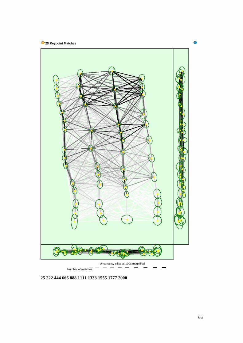
66

25 222 444 666 888 1111 1333 1555 1777 2000

2 D Keypoint Matches

Uncertainty ellipses 100x magnified

Number of matches

67

Figure 5: Computed image positions with links between matched images. The

darkness of the links indicates the number of matched 2D keypoints between the

images. Bright links indicate weak links and require manual tie points or more

images. Dark green ellipses indicate the relative camera position uncertainty of the

bundle block adjustment result.

Relative camera position and orientation uncertainties

Hardware

CPU: Intel(R) Core(TM) i7-3632QM CPU @ 2.20GHz

RAM: 8GB

GPU: Intel(R) HD Graphics 4000 (Driver: 10.18.10.4276)

Operating System Windows 10 Home, 64-bit

Coordinate Systems

Ground Control Point (GCP) Coordinate System Arbitrary (m)

Output Coordinate System Arbitrary (m)

Processing Options

Detected Template No Template Available

Keypoints Image Scale Full, Image Scale: 1

Advanced: Matching Image Pairs Aerial Grid or Corridor

Advanced: Matching Strategy Use Geometrically Verified Matching: no

Advanced: Keypoint Extraction Targeted Number of Keypoints: Automatic

X

[m]

Y

[m]

Z [m] Omega [degree] Phi [degree] Kappa [degree]

Mean 0.018 0.025 0.016 0.064 0.045 0.014

Sigma 0.005 0.006 0.007 0.028 0.018 0.003

Initial Processing Details

System Information

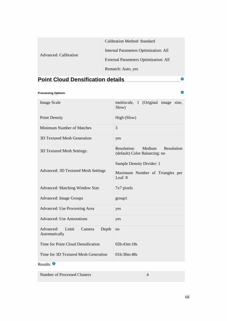
68

Advanced: Calibration

Calibration Method: Standard

Internal Parameters Optimization: All

External Parameters Optimization: All

Rematch: Auto, yes

Image Scale multiscale, 1 (Original image size,

Slow)

Point Density High (Slow)

Minimum Number of Matches 3

3D Textured Mesh Generation yes

3D Textured Mesh Settings: Resolution: Medium Resolution

(default) Color Balancing: no

Advanced: 3D Textured Mesh Settings

Sample Density Divider: 1

Maximum Number of Triangles per

Leaf: 8

Advanced: Matching Window Size 7x7 pixels

Advanced: Image Groups group1

Advanced: Use Processing Area yes

Advanced: Use Annotations yes

Advanced: Limit Camera Depth

Automatically

no

Time for Point Cloud Densification 02h:43m:18s

Time for 3D Textured Mesh Generation 01h:30m:48s

Results

Number of Processed Clusters 4

Point Cloud Densification details

Processing Options

69

Number of Generated Tiles 4

Number of 3D Densified Points 71018183

Average Density (per m3) 9902.38

DSM and Orthomosaic Resolution 1 x GSD (1.31 [cm/pixel])

DSM Filters Noise Filtering: yes

Surface Smoothing: yes, Type: Sharp

Grid DSM Generated: yes, Spacing [cm]: 1

Time for DSM Generation 51m:44s

DSM, Orthomosaic and Index Details

Processing Options

70

Generated with Pro version 2.2.25

Important: Click on the different icons for:

Help to analyze the results in the Quality Report

Additional information about the sections

Click here for additional tips to analyze the Quality Report

Summary

Project project test #16 portrait

Processed 2016-10-10 06:19:37

Camera Model Name(s) NEX-5N_E18-55mmF3.5-

5.6OSS_19.0_4912x3264 (RGB)

Average Ground Sampling

Distance (GSD)

1.3 cm / 0.51 in

Area Covered 0.0125 km2 / 1.2513 ha / 0.0048 sq. mi. / 3.0937

acres

Quality Check

Images median of 54778 keypoints per image

Dataset 62 out of 63 images calibrated (98%), all images enabled

Camera

Optimization

3.15% relative difference between initial and optimized

internal camera parameters

Matching median of 7642.55 matches per calibrated image

Georeferencing yes, 6 GCPs (6 3D), mean RMS error = 0.009 m

Quality Report

Preview

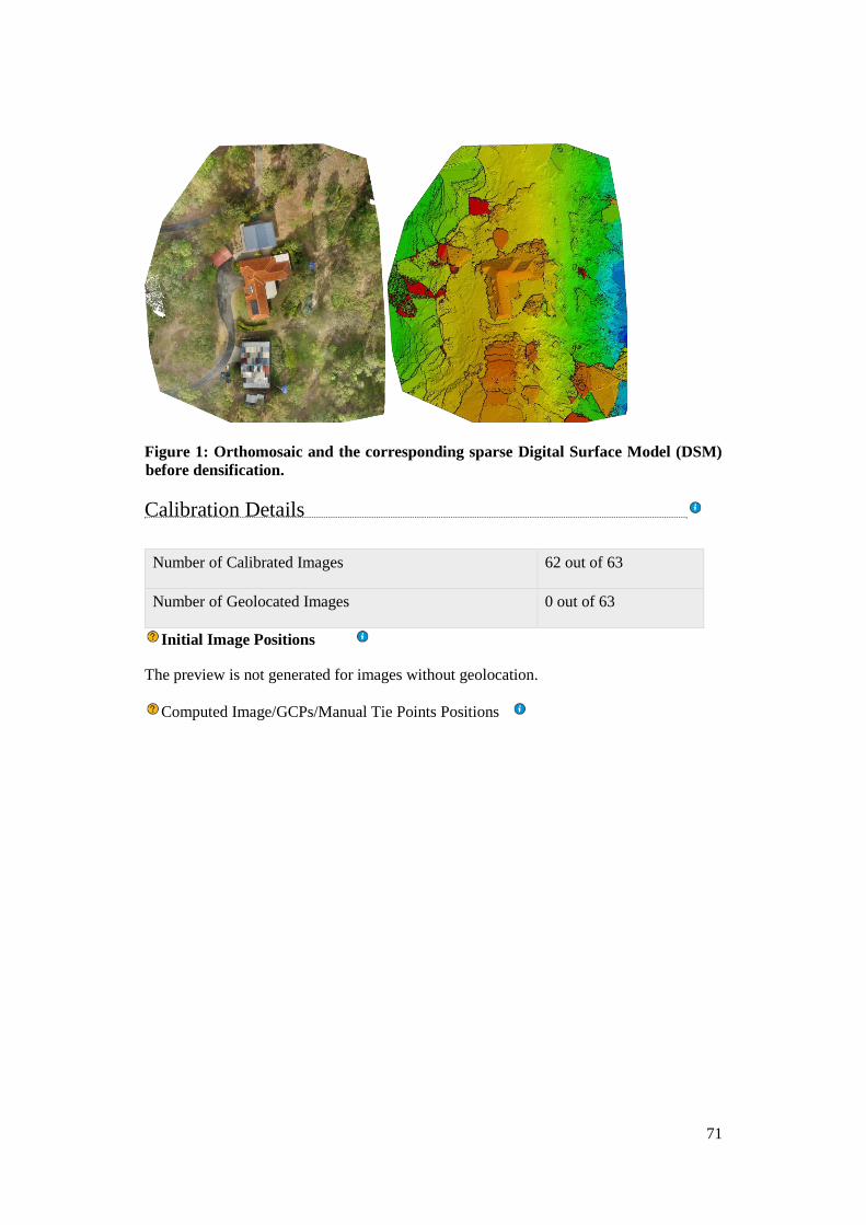
71

Figure 1: Orthomosaic and the corresponding sparse Digital Surface Model (DSM)

before densification.

Number of Calibrated Images 62 out of 63

Number of Geolocated Images 0 out of 63

Initial Image Positions

The preview is not generated for images without geolocation.

Computed Image/GCPs/Manual Tie Points Positions

Calibration Details

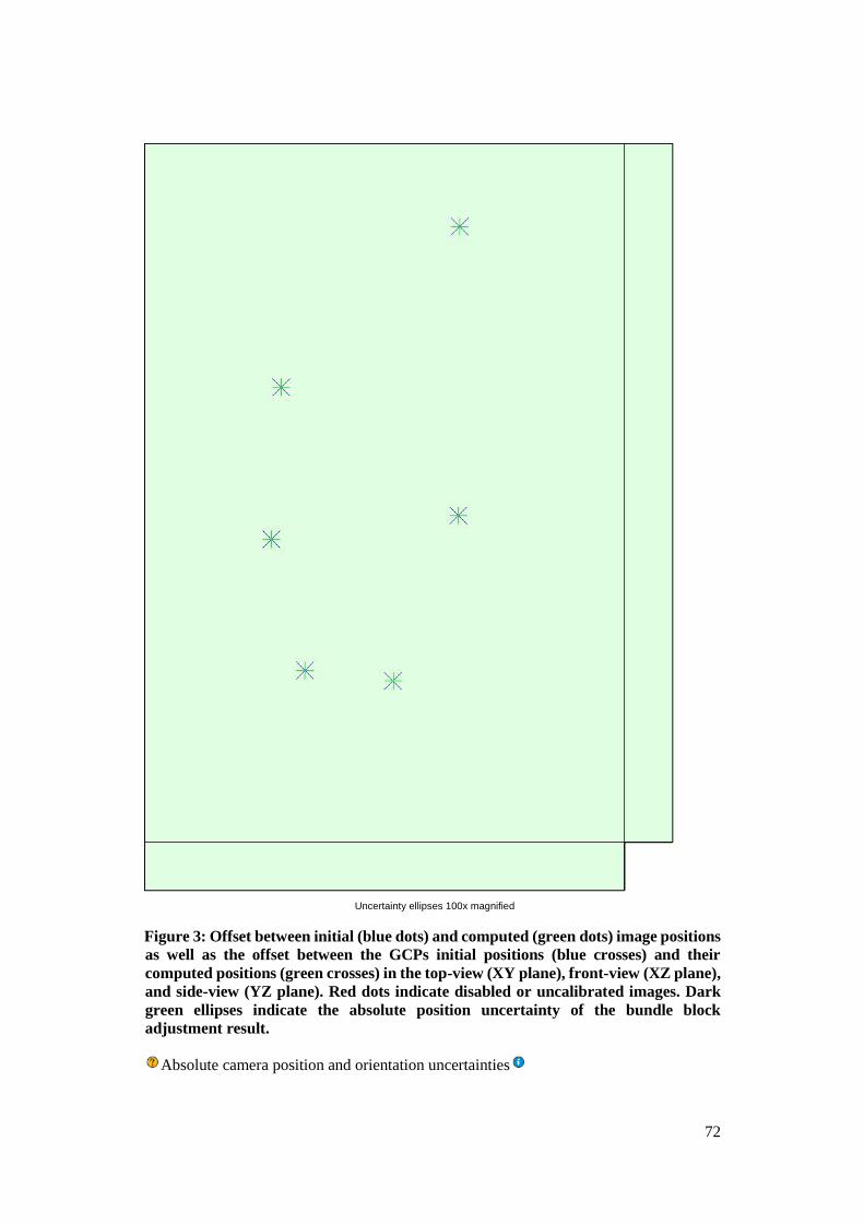
72

Figure 3: Offset between initial (blue dots) and computed (green dots) image positions

as well as the offset between the GCPs initial positions (blue crosses) and their

computed positions (green crosses) in the top-view (XY plane), front-view (XZ plane),

and side-view (YZ plane). Red dots indicate disabled or uncalibrated images. Dark

green ellipses indicate the absolute position uncertainty of the bundle block

adjustment result.

Absolute camera position and orientation uncertainties

Uncertainty ellipses 100x magnified

73

X

[m]

Y

[m]

Z [m] Omega [degree] Phi [degree] Kappa [degree]

Mean 0.030 0.030 0.129 0.034 0.031 0.009

Sigma 0.006 0.011 0.005 0.011 0.006 0.003

Overlap

Figure 4: Number of overlapping images computed for each pixel of the orthomosaic.

Red and yellow areas indicate low overlap for which poor results may be generated.

Green areas indicate an overlap of over 5 images for every pixel. Good quality results

will be generated as long as the number of keypoint matches is also sufficient for these

areas (see Figure 5 for keypoint matches).

Number of 2D Keypoint Observations for Bundle Block Adjustment 520091

Number of 3D Points for Bundle Block Adjustment 190586

Mean Reprojection Error [pixels] 0.163

Number of overlapping images: 1 2 3 4 5+

Bundle Block Adjustment Details

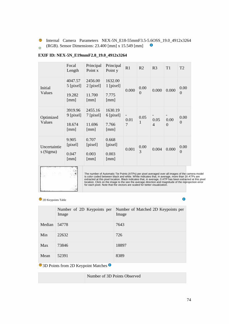
74

Internal Camera Parameters NEX-5N_E18-55mmF3.5-5.6OSS_19.0_4912x3264

(RGB). Sensor Dimensions: 23.400 [mm] x 15.549 [mm]

EXIF ID: NEX-5N_E19mmF2.8_19.0_4912x3264

Focal

Length

Principal

Point x

Principal

Point y R1 R2 R3 T1 T2

Initial

Values

4047.57

5 [pixel]

19.282

[mm]

2456.00

2 [pixel]

11.700

[mm]

1632.00

1 [pixel]

7.775

[mm]

0.000 0.00

0 0.000 0.000

0.00

0

Optimized

Values

3919.96

9 [pixel]

18.674

[mm]

2455.16

7 [pixel]

11.696

[mm]

1630.19

6 [pixel]

7.766

[mm]

-

0.01

7

0.05

1

-

0.05

4

-

0.00

0

0.00

0

Uncertaintie

s (Sigma)

9.905

[pixel]

0.047

[mm]

0.707

[pixel]

0.003

[mm]

0.668

[pixel]

0.003

[mm]

0.001 0.00

3 0.004 0.000

0.00

0

Number of 2D Keypoints per

Image

Number of Matched 2D Keypoints per

Image

Median 54778 7643

Min 22632 726

Max 73846 18897

Mean 52391 8389

3D Points from 2D Keypoint Matches

Number of 3D Points Observed

The number of Automatic Tie Points (ATPs) per pixel averaged over all images of the camera model is color coded between black and white. White indicates that, in average, more than 16 ATPs are extracted at this pixel location. Black indicates that, in average, 0 ATP has been extracted at this pixel location. Click on the image to the see the average direction and magnitude of the reprojection error for each pixel. Note that the vectors are scaled for better visualization.

2 D Keypoints Table

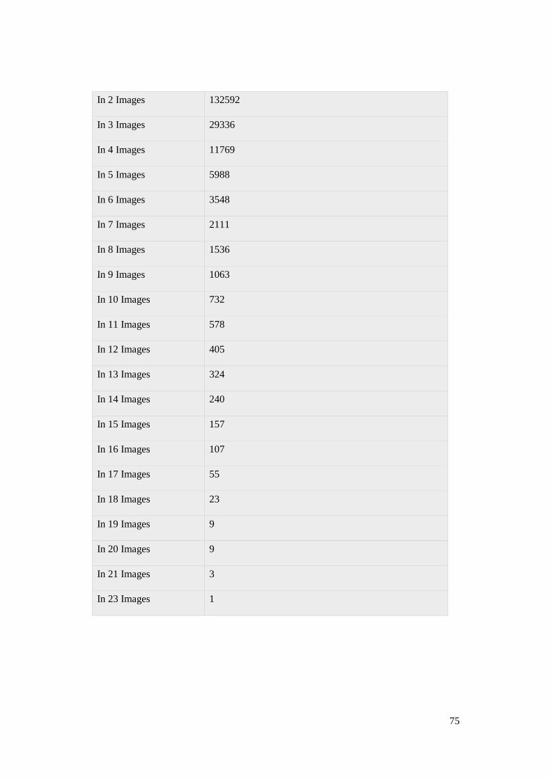
75

In 2 Images 132592

In 3 Images 29336

In 4 Images 11769

In 5 Images 5988

In 6 Images 3548

In 7 Images 2111

In 8 Images 1536

In 9 Images 1063

In 10 Images 732

In 11 Images 578

In 12 Images 405

In 13 Images 324

In 14 Images 240

In 15 Images 157

In 16 Images 107

In 17 Images 55

In 18 Images 23

In 19 Images 9

In 20 Images 9

In 21 Images 3

In 23 Images 1

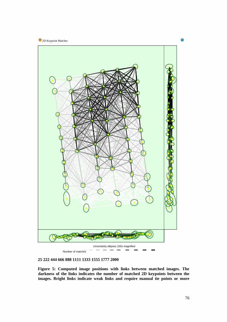
76

25 222 444 666 888 1111 1333 1555 1777 2000

Figure 5: Computed image positions with links between matched images. The

darkness of the links indicates the number of matched 2D keypoints between the

images. Bright links indicate weak links and require manual tie points or more

2 D Keypoint Matches

Uncertainty ellipses 100x magnified

Number of matches

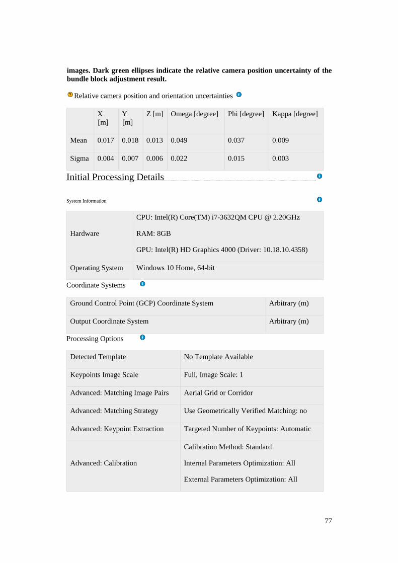
77

images. Dark green ellipses indicate the relative camera position uncertainty of the

bundle block adjustment result.

Relative camera position and orientation uncertainties

X

[m]

Y

[m]

Z [m] Omega [degree] Phi [degree] Kappa [degree]

Mean 0.017 0.018 0.013 0.049 0.037 0.009

Sigma 0.004 0.007 0.006 0.022 0.015 0.003

Hardware

CPU: Intel(R) Core(TM) i7-3632QM CPU @ 2.20GHz

RAM: 8GB

GPU: Intel(R) HD Graphics 4000 (Driver: 10.18.10.4358)

Operating System Windows 10 Home, 64-bit

Coordinate Systems

Ground Control Point (GCP) Coordinate System Arbitrary (m)

Output Coordinate System Arbitrary (m)

Processing Options

Detected Template No Template Available

Keypoints Image Scale Full, Image Scale: 1

Advanced: Matching Image Pairs Aerial Grid or Corridor

Advanced: Matching Strategy Use Geometrically Verified Matching: no

Advanced: Keypoint Extraction Targeted Number of Keypoints: Automatic

Advanced: Calibration

Calibration Method: Standard

Internal Parameters Optimization: All

External Parameters Optimization: All

Initial Processing Details

System Information

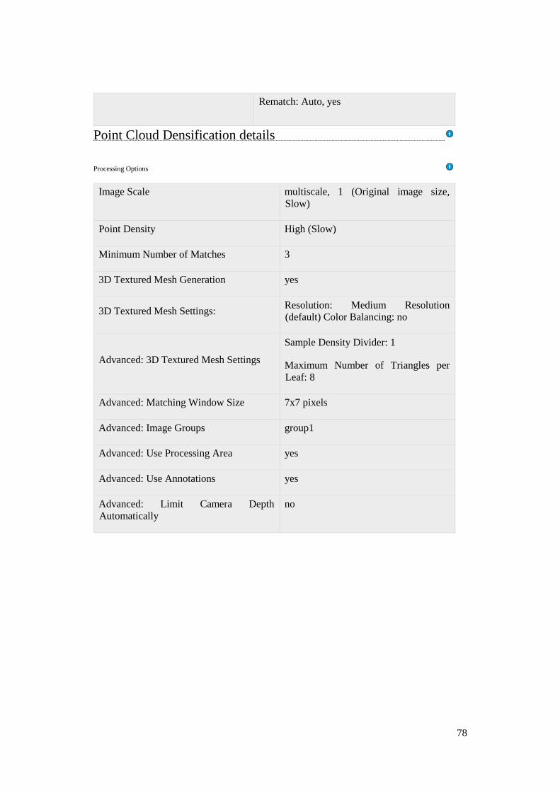
78

Rematch: Auto, yes

Image Scale multiscale, 1 (Original image size,

Slow)

Point Density High (Slow)

Minimum Number of Matches 3

3D Textured Mesh Generation yes

3D Textured Mesh Settings: Resolution: Medium Resolution

(default) Color Balancing: no

Advanced: 3D Textured Mesh Settings

Sample Density Divider: 1

Maximum Number of Triangles per

Leaf: 8

Advanced: Matching Window Size 7x7 pixels

Advanced: Image Groups group1

Advanced: Use Processing Area yes

Advanced: Use Annotations yes

Advanced: Limit Camera Depth

Automatically

no

Point Cloud Densification details

Processing Options