P O S I V A O Y

FIN-27160 OLKILUOTO, F INLAND

Tel +358-2-8372 31

Fax +358-2-8372 3709

Jorma Pa lménT i i na Va i t t i nenHenry Ahokas

Jorma NummelaEero He ikk inen

November 2004

Work ing Repor t 2004 -53

3D Model of Salinityof Bedrock Groundwater

at Olkiluoto

November 2004

Working Reports contain information on work in progress

or pending completion.

The conclusions and viewpoints presented in the report

are those of author(s) and do not necessarily

coincide with those of Posiva.

Jorma Pa lmén

T i i na Va i t t i nen

Henry Ahokas

Jorma Nummela

Eero He ikk inen

JP-F in tac t Oy

Work ing Report 2004 -53

3D Model of Salinityof Bedrock Groundwater

at Olkiluoto

Palmén J., Vaittinen T., Ahokas H., Nummela J., & Heikkinen E. 2004. 3D-model of

salinity of bedrock groundwater at Olkiluoto. Posiva Oy. Working report 2004-53. 92 p.

ABSTRACT

Posiva carries out investigations and preparations for spent nuclear fuel disposal

into Finnish bedrock at Olkiluoto. The salinity of groundwater in the bedrock, its

distribution and quantity are important factors in planning the facilities for final disposal

of the spent nuclear fuel, and in assessing the functionality and safety of the facilities.

Belonging to site investigations, JP-Fintact carried out compilation of 3-D volume

model of total dissolved salinity (TDS, g/l) distribution of Olkiluoto site. The model

covers the central part of Olkiluoto island bedrock volume. The model update replaces

the previous works. Current model is more simplified presentation of observations than

previously, containing essentially enhanced amount and coverage of TDS data.

The model is based on the hydrochemical TDS observations and the hydrology

groundwater electrical conductivity data of flow logging converted to TDS.

Observations confirm the concept of layered, diffuse behavior of increasing salinity

according to depth. Model has been presented with four salinity classes (<1 g/l, 1-10 g/l,

10-30 g/l and >30 g/l), and two boundary surfaces have been shown between the

volumes occupied by these classes. The boundaries are subhorizontal. The local

distribution is heterogeneous, and its description will benefit of new data when

available.

The indirect geophysical electrical borehole logging and electromagnetic

frequency sounding observation data offers dense data coverage, also outside of other

borehole observations and the volume covered by boreholes. The usage was based on

the ratio of groundwater electrical conductivity and TDS, and on the dependencies

between bedrock electrical conductivity, porosity and groundwater electrical

conductivity. The geophysical data values have variability compared to the model.

The gathered TDS observations have been compiled into TDS boundaries and

layers into Posiva’s ROCK-CAD system. Graphical presentations of the model have

been compiled. The model has then been referred to the original geochemical and

hydrological data, and to the site fracture zone model. Fracture zones seem to have some

control of the local salinity distribution.

The report describes the data and their use, and the compilation of model and the

results. The model can now be used for later assessment, comparisons and visualization.

Keywords: Groundwater salinity, 3D-model, ROCK-CAD.

Palmén J., Vaittinen T., Ahokas H., Nummela J., & Heikkinen E. 2003. Olkiluodon

tutkimusalueen pohjavesien suolaisuuden tilavuusmalli. Posiva Oy, Työraportti 2004-53.

92s.

TIIVISTELMÄ

Posiva huolehtii korkea-aktiivisen käytetyn ydinpolttoaineen loppusijoituksen

tutkimus- ja valmistelutehtävistä Olkiluodossa. Kallioperässä sijaitsevan pohjaveden

suolaisuus, sijainti ja määrä ovat oleellisia tekijöitä suunniteltaessa ja rakennettaessa

käytetyn ydinpolttoaineen loppusijoitustiloja sekä arvioitaessa niiden toimivuutta ja

turvallisuutta.

Tutkimuksiin liittyen on JP-Fintact Oy:ssä laadittu Olkiluodon tutkimusaineiston

pohjalta kalliopohjavesien kokonaissuolapitoisuuden (TDS, g/l) vaihtelun kolmiulottei-

nen tilavuusmalli. Malli kattaa Olkiluodon saaren keskiosan kalliotilavuuden ja korvaa

aikaisemmat esitykset, sisältäen oleellisesti lisääntyneen määrän ja kattavampaa TDS-

dataa kuin aiemmin.

Mallin lähtöaineistona on käytetty pohjavesikemian suolaisuushavaintoja, ja

virtausmittausten veden sähkönjohtavuuden laskennallisia suolaisuushavaintoja. Havain-

not vahvistavat käsitystä kerrosmaisesta, vaihettuvin rajapinnoin syvyyden suhteen

kasvavasta suolaisuudesta. Mallissa on esitetty neljä suolaisuuden luokkaa (<1 g/l, 1-10

g/l, 10-30 g/l ja >30 g/l), ja kaksi niiden välistä rajapintaa. Rajapinnat on esitetty

tasomaisina ja ne ovat melko vaaka-asentoisia. Paikallisesti suolaisuusjakauma on

heterogeeninen, ja sen ominaisuuksista saadaan lisätietoa uusien tutkimusten tuloksista.

Epäsuora geofysiikan sähköisten reikämittausten ja sähkömagneettisten

taajuusluotausten havaintopisteaineisto on tiheä ja laajentaa tuloksia reikähavaintojen

sekä reikien kattaman tilavuuden ulkopuolelle. Aineiston käyttö perustuu pohjaveden

ominaisvastuksen ja kokonaissuolapitoisuuden, sekä kallion ominaisvastuksen,

huokoisuuden ja veden ominaisvastuksen välisiin riippuvuuksiin. Geofysiikan tulokset

osoittavat vaihtelua koottuun malliin nähden.

Kerätyt suolaisuusviitteet on koottu TDS-vaihtelun rajapinnoiksi ja tilavuusmallin

osiksi Posiva Oy:n ROCK-CAD -järjestelmään, jossa mallista on myös laadittu graafiset

esitykset. Mallia on myös verrattu geohydrologiseen ja pohjavesikemialliseen

lähtöaineistoon sekä tutkimusalueen rako- ja rikkonaisuusyksiköihin. Rikkonaisuus-

vyöhykkeillä näyttäisi olevan jonkin verran vaikutusta suolaisuuden jakaumaan.

Raportissa on kuvattu lähtöaineistot ja niiden käyttö sekä mallin luonti, kuvaus ja

arviointi. Malli on käytettävissä myöhempiin arviointeihin, vertailuihin ja havainnol-

listukseen.

Avainsanat: Pohjaveden suolaisuus, tilavuusmalli, ROCK-CAD.

1

TABLE OF CONTENTS

ABSTRACT

TIIVISTELMÄ

TABLE OF CONTENTS ..................................................................................... 1

1 INTRODUCTION .......................................................................................... 3

2 PREVIOUS STUDIES................................................................................... 5

3 RELATIONS AND EQUATIONS .................................................................. 7

4 HYDROCHEMICAL DATA ........................................................................... 9

4.1 Groundwater sampling .................................................................................................................9

4.2 Sampling in multipackered boreholes .........................................................................................9

4.3 Double packer system for open boreholes.................................................................................10

4.4 Pressurized groundwater samples with the PAVE sampler ....................................................12

4.5 Processing and control of the data quality ................................................................................14

5 DIFFERENCE FLOW METER DATA ......................................................... 21

5.1 Description of the difference flow meter ...................................................................................21

5.2 Description of the in situ EC measurement ..............................................................................21

5.3 Quality control of in situ EC-measurements.............................................................................23

5.4 Reference data .............................................................................................................................24

5.5 Processing of the data .................................................................................................................24

5.6 Comparison of in situ data to hydrochemical data ..................................................................27

2

6 GEOPHYSICAL DATA............................................................................... 29

6.1 Long normal resistivity logging data .........................................................................................31

6.1.1 Reference data .....................................................................................................................366.1.2 Processing of the data .........................................................................................................36

6.2 GEOPHYSICAL ELECTROMAGNETIC GEFINEX 400S DATA ......................................39

6.2.1 The GEFINEX 400S method...............................................................................................396.2.2 The data ...............................................................................................................................426.2.3 Quality control of the Gefinex 400S data ............................................................................436.2.4 Reference data .....................................................................................................................446.2.5 Processing of the data .........................................................................................................44

7 3D SALINITY MODEL ................................................................................ 47

7.1 Boundary surfaces.......................................................................................................................49

7.1.1 Modelling method................................................................................................................497.1.2 Boundary surface, TDS 1 g/l ...............................................................................................527.1.3 Boundary surface, TDS 10 g/l .............................................................................................52

7.2 Salinity distribution of major structures...................................................................................57

7.3 Volumetric salinity model...........................................................................................................61

8 DISCUSSION.............................................................................................. 65

9 REFERENCES ........................................................................................... 69

APPENDICES................................................................................................... 77

1. Difference Flow meter data source reports..........................................................................................79

2. Geophysical long normal resistivity logging data reports ...................................................................80

3. Geophysical long normal and borehole fluid conductivity results with in situ EC values, from boreholes KR1, KR2, KR4, KR7, KR9, KR11, KR12 and KR19. ..............................................................81

4. Geophysical long normal EC values visualized along with model boundaries ...................................89

5. Geophysical GEFINEX 400S EC values visualized along with model boundaries.............................92

3

1 INTRODUCTION

Posiva carries out investigations and preparations for spent nuclear fuel disposal into

Finnish bedrock at Olkiluoto. Construction of ONKALO underground disposal facilities

will commence in summer 2004.

The distribution and quantity of saline groundwater are important factors in planning the

facilities for final disposal of the spent nuclear fuel, and in assessing the functionality

and safety of the facilities. Existing investigation data will be visualized within the site

volume for planning and design purposes, and to allow follow-up of changes in

properties during construction.

The task of this work was to gather up, verify and display all possible spatial data

available of salinity at the time of preparing the work. The task was to create model and

visualize the distribution of groundwater salinity in the Olkiluoto bedrock volume. The

work consisted of gathering up the groundwater geochemical, hydrological and

geophysical information of groundwater salinity measurements (TDS, total dissolved

solids) and geophysical indications (electrical conductivity) of groundwater salinity

spatial distribution into a volumetric model.

The groundwater geochemical data (Helenius 1998, Karttunen et al. 1999, 2000,

Snellman 1991, Snellman et al. 1995, Karttunen & Mäntynen 2001, Paaso & Mäntynen

2002, Rantanen et al. 2002, Tuominen 1995, Palmén & Hellä 2003) from KR1-KR14

was assigned with geometrical location and assessed with quality control (Chapter 4,

Jorma Palmén).

The hydrological detailed difference flow data of electrical conductivity (EC) from the

KR1-KR23 boreholes (Rouhiainen 1999, Pöllänen & Rouhiainen 2000, 2001a,b,

2002a,b) was compared to the hydrogeochemical data, and converted to TDS values

(Chapter 5, Henry Ahokas and Jorma Palmén).

The geophysical long normal electrical logging data (e.g. Julkunen et al. 2000b, see

Table 1 for other references) was converted to TDS values as well. A largest scale of

data set, geophysical electromagnetic frequency sounding interpretations (Jokinen et al.

1995; Heikkinen et al. 2004a), were gathered up and the bedrock resistivities were

converted to TDS values (Chapter 6, Eero Heikkinen and Jorma Palmén).

The obtained TDS data, with their coordinates, were imported to CAD modeling system

(ROCK-CAD), and visualized with their quality and certainty level properties. Then the

observations were merged to simplified geometrical objects by means of interpolating

4

TDS boundary surfaces for four different salinity classes from fresh waters to brine. The

results were visualized in form of maps, vertical cross sections with boreholes and with

structural model, together with the observed data. (Chapter 7, Tiina Vaittinen and Jorma

Nummela).

Commentary of the salinity distribution was prepared into Chapter 8 (Ahokas, Vaittinen,

Palmén, Heikkinen). It has to be noted that the work will consider the bedrock contain

similar salinity properties as the samples, which are taken from fracture zones where

water has been freely available for sampling.

Mr Jorma Palmén gathered up and analysed all the borehole data, and wrote the report.

The model and visualizations was created by, and interpretations performed by Mrs.

Tiina Vaittinen. The work was designed by Mr. Eero Heikkinen. Mr Henry Ahokas was

responsible for hydrological data review. The design of CAD routines for model

construction was created by Mr. Jorma Nummela. Electromagnetic sounding data was

provided and reviewed by Mr Turo Ahokas, Posiva.

5

2 PREVIOUS STUDIES

The groundwater geochemical sampling has been performed in the boreholes since early

1990’s. Parallel to the analyses, the groundwater types and their distributions have been

described at several stages and modelled with transport and evolution models (Pitkänen

et al. 1992, 1993, 1994, 1996, 1999, Lampén 1993, Lampén & Snellman 1993,

Ruotsalainen & Snellman 1996, Löfman 1999, Luukkonen et al. 2003). Other

investigations on the water species are e.g. (Blomqvist 1999, Blomqvist et al 1992, Blyth

et al. 1998, Frape & Fritz 1987, Casgoyne et al. 1996, Laaksoharju 1999, Nordstrom

1989, Savoye et al. 1998). Supporting data sets from hydrological and geophysical

methods have been obtained and analysed in several phases.

The geophysical electrical and electromagnetic sounding interpretations have been

assessed for bedrock groundwater salinity during the actual processing (Paananen et al.

1991, Jokinen et al. 1995). The results were also converted to represent the groundwater

salinity and created to volumetric objects in 1996 (Heikkinen et al. 1996), based on the

level of knowledge in that time. It was recognized, though, that part of the electrical

conductivity observations were related rather to pyrite and graphite horizons in host rock

than any saline water interfaces or bodies. Both geochemical and geophysical data sets

were rather limited in that time.

With more detailed geochemical and hydrological EC data available from KR1-KR11,

the data was visualized and its quality assessed, and compared to the fracture data in

2000 (Ruotsalainen et al. 2000). The results were also compared to the salinity model of

1996. There were differences observed in the data to the previous model. The chemical

composition of the water species, and their relation to EC and TDS, have been modeled

with synthetic samples (Mäntynen 2000), and the mathematical relationship between EC

and TDS has been deduced (Heikkonen et al. 2002). Both these works have been utilized

in this approach.

The amount of data has increased significantly with boreholes KR12-KR23, and added

with new EM soundings (Ahokas 2003) and their interpretations (Heikkinen et al.

2004a). Also the spatial distribution and evolution of the water types have been analysed

more recently (Luukkonen et al. 2003). This work concentrates to visualize the

observations into a model, which allows presentation of cross sections, without taking

into account the actual water species, their relationships or distributions. The

classification is based on the work presented in Davis (1964).

The visualisation and model compilation has a significant simplification inherent. Most

of the data is obtained from groundwater taken from fractures and fracture zones. It is

6

assumed that the water in the host rock (pores, fractures) not penetrated with a borehole

or a major fracture zone, would contain similar groundwater as that observed in the

sampling and investigations. There are some indications that this assumption may not

uniquely be valid in certain conditions and locations. It also seems out, that the

investigations have already interfered with the volume properties. Flow may have

introduced waters of different salinities than originally have existed in the bedrock

volume studied.

Other similar works have been recently reported from permafrost investigations of Lupin

mine (Paananen & Ruskeeniemi 2003), groundwater salinitization mapping from

airborne electromagnetic investigations from Texas (Paine & Collins 2003), and similar

approach of Hästholmen electromagnetic frequency sounding interpretations (Paananen

et al. 1998); where the electrical conductivity of bedrock is mainly due to fracturing and

saline groundwater.

7

3 RELATIONS AND EQUATIONS

In this study, all EC(in situ) measurements have used the same correlation procedure for

converting EC results to 25°C and to TDS (Heikkonen et al. 2002). Other correlation

functions have been applied over time, e.g. the SFS standard correlation, and Olkiluoto-

specific correlation (1) between measured EC(chem) (mS/m) values and the TDS (g/l)

values from the hydrochemical studies (Ruotsalainen et al. 2000).

TDS = 8.358•10-8 • (EC(chem))2 + 5.9927•10-3 • (EC(chem)) (1)

In the hydrochemical studies the TDS values of the water samples were calculated using

the analysed concentrations of all cations, anions, total iron and silica. The chemical

names and formulae of the ions (all in g/l) are listed in order of their respective

concentrations in (2) (e.g. Hounslow 1995):

TDS = HCO3 + CO3 + CO2(free) + SiO2 + Fetot + Al + Na + K + Ca + Mg + Mn + Rb + Sr

+ Li + Ba + Cs + B + S2- + SO4 + PO4 + NH4+ + NO2 + NO3 + Cl + F + Br + I

[g/l] (2)

There is a general correlation of EC (mS/m) and salinity as TDS (g/l) induced by NaCl

(e.g. Hounslow 1995):

TDS(NaCl) = 6.5•10-3 • EC [g/l] (3)

The electrical conductivity of the rock mass is related to water content, the conductivity

of water, and the pore space. The total porosity nt of a fractured medium (Poikonen

1983b, Brace et al.1965) can be expressed as

nt = nf + np (4)

Where nf is fracture porosity and np is pore porosity. Most of the electrical current flows

through the interstial fluid. Thus the electrical conductivity can be decomposed into

three components:

- conduction along fractures

- conduction through pores and

- surface conduction (thin water films on surfaces; due to excess of ions at solid-liquid

interfaces)

8

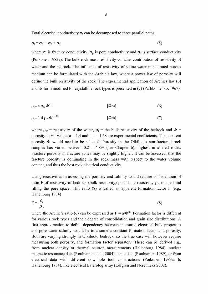
Total electrical conductivity σt can be decomposed to three parallel paths,

σt = σf + σp + σs (5)

where σf is fracture conductivity, σp is pore conductivity and σs is surface conductivity

(Poikonen 1983a). The bulk rock mass resistivity contains contribution of resistivity of

water and the bedrock. The influence of resistivity of saline water in saturated porous

medium can be formulated with the Archie’s law, where a power law of porosity will

define the bulk resistivity of the rock. The experimental application of Archies law (6)

and its form modified for crystalline rock types is presented in (7) (Parhkomenko, 1967).

ρt = a ρwΦm [Ωm] (6)

ρt = 1.4 ρwΦ-1.58 [Ωm] (7)

where ρw = resistivity of the water, ρt = the bulk resistivity of the bedrock and Φ =

porosity in %. Values a = 1.4 and m = –1.58 are experimental coefficients. The apparent

porosity Φ would need to be selected. Porosity in the Olkiluoto non-fractured rock

samples has varied between 0.2 – 6.8% (see Chapter 6), highest in altered rocks.

Fracture porosity in fracture zones may be slightly higher. It can be assessed, that the

fracture porosity is dominating in the rock mass with respect to the water volume

content, and thus the host rock electrical conductivity.

Using resistivities in assessing the porosity and salinity would require consideration of

ratio F of resistivity of bedrock (bulk resistivity) ρt and the resistivity ρw of the fluid

filling the pore space. This ratio (8) is called an apparent formation factor F (e.g.,

Hallenburg 1984)

F = w

t

ρρ

(8)

where the Archie’s ratio (6) can be expressed as F = a/Φm. Formation factor is different

for various rock types and their degree of consolidation and grain size distributions. A

first approximation to define dependency between measured electrical bulk properties

and pore water salinity would be to assume a constant formation factor and porosity.

Both are varying strongly in Olkiluoto bedrock, so the true case will however require

measuring both porosity, and formation factor separately. These can be derived e.g.,

from nuclear density or thermal neutron measurements (Hallenburg 1984), nuclear

magnetic resonance data (Rouhiainen et al. 2004), sonic data (Rouhiainen 1989), or from

electrical data with different downhole tool constructions (Poikonen 1983a, b,

Hallenburg 1984), like electrical Laterolog array (Löfgren and Neretnieks 2002).

9

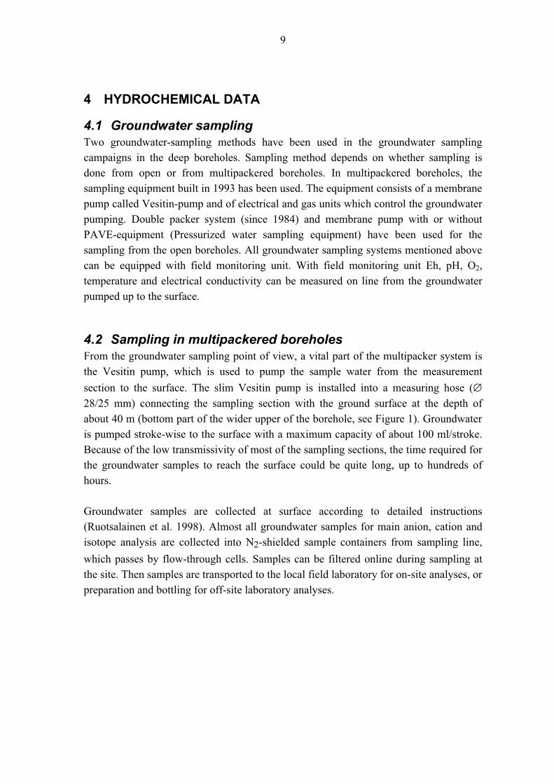
4 HYDROCHEMICAL DATA

4.1 Groundwater sampling

Two groundwater-sampling methods have been used in the groundwater sampling

campaigns in the deep boreholes. Sampling method depends on whether sampling is

done from open or from multipackered boreholes. In multipackered boreholes, the

sampling equipment built in 1993 has been used. The equipment consists of a membrane

pump called Vesitin-pump and of electrical and gas units which control the groundwater

pumping. Double packer system (since 1984) and membrane pump with or without

PAVE-equipment (Pressurized water sampling equipment) have been used for the

sampling from the open boreholes. All groundwater sampling systems mentioned above

can be equipped with field monitoring unit. With field monitoring unit Eh, pH, O2,

temperature and electrical conductivity can be measured on line from the groundwater

pumped up to the surface.

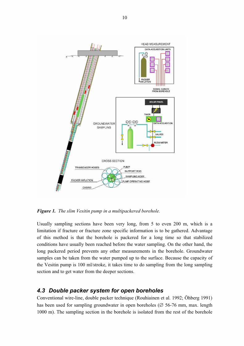
4.2 Sampling in multipackered boreholes

From the groundwater sampling point of view, a vital part of the multipacker system is

the Vesitin pump, which is used to pump the sample water from the measurement

section to the surface. The slim Vesitin pump is installed into a measuring hose (∅28/25 mm) connecting the sampling section with the ground surface at the depth of

about 40 m (bottom part of the wider upper of the borehole, see Figure 1). Groundwater

is pumped stroke-wise to the surface with a maximum capacity of about 100 ml/stroke.

Because of the low transmissivity of most of the sampling sections, the time required for

the groundwater samples to reach the surface could be quite long, up to hundreds of

hours.

Groundwater samples are collected at surface according to detailed instructions

(Ruotsalainen et al. 1998). Almost all groundwater samples for main anion, cation and

isotope analysis are collected into N2-shielded sample containers from sampling line,

which passes by flow-through cells. Samples can be filtered online during sampling at

the site. Then samples are transported to the local field laboratory for on-site analyses, or

preparation and bottling for off-site laboratory analyses.

10

Figure 1. The slim Vesitin pump in a multipackered borehole.

Usually sampling sections have been very long, from 5 to even 200 m, which is a

limitation if fracture or fracture zone specific information is to be gathered. Advantage

of this method is that the borehole is packered for a long time so that stabilized

conditions have usually been reached before the water sampling. On the other hand, the

long packered period prevents any other measurements in the borehole. Groundwater

samples can be taken from the water pumped up to the surface. Because the capacity of

the Vesitin pump is 100 ml/stroke, it takes time to do sampling from the long sampling

section and to get water from the deeper sections.

4.3 Double packer system for open boreholes

Conventional wire-line, double packer technique (Rouhiainen et al. 1992; Öhberg 1991)

has been used for sampling groundwater in open boreholes (∅ 56-76 mm, max. length

1000 m). The sampling section in the borehole is isolated from the rest of the borehole

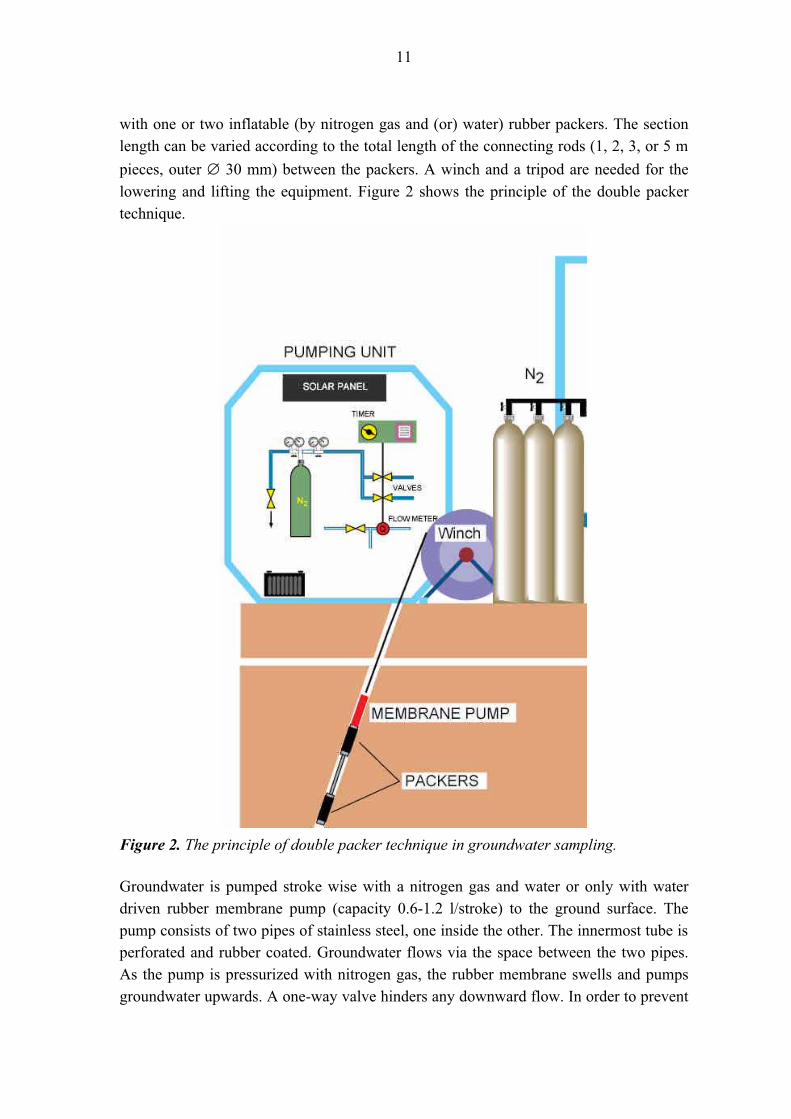
11

with one or two inflatable (by nitrogen gas and (or) water) rubber packers. The section

length can be varied according to the total length of the connecting rods (1, 2, 3, or 5 m

pieces, outer ∅ 30 mm) between the packers. A winch and a tripod are needed for the

lowering and lifting the equipment. Figure 2 shows the principle of the double packer

technique.

Figure 2. The principle of double packer technique in groundwater sampling.

Groundwater is pumped stroke wise with a nitrogen gas and water or only with water

driven rubber membrane pump (capacity 0.6-1.2 l/stroke) to the ground surface. The

pump consists of two pipes of stainless steel, one inside the other. The innermost tube is

perforated and rubber coated. Groundwater flows via the space between the two pipes.

As the pump is pressurized with nitrogen gas, the rubber membrane swells and pumps

groundwater upwards. A one-way valve hinders any downward flow. In order to prevent

12

direct contact of nitrogen gas and the rubber membrane, the inner pipe and the pressure

hose have been filled with water to a desired depth, which depends on the sampling

depth, on the level of the groundwater and on the working pressure of pumping. Usually

only 5-10 m of the hose is left empty for N2 gas. In the filling of the membrane pump

pressure is reduced and water flows from the fractures to the sampling section. The

magnitude of the suction pressure corresponds to the difference in water levels between

the groundwater table and the pressure hose. The maximum permitted suction pressure is

10 bars. The membrane pump is operated with solenoid valves, a timer, time relays and

a pulse counter on the ground level. The length of the filling time depends on the

permeability of the rock and the length and diameter of the hose system used. The length

of the draining time depends on the length and diameter of the hoses. Both the filling

and the draining take typically some minutes for each.

Before 1997, the double packer system was used to do groundwater sampling from open

boreholes. After year 1997 the PAVE-sampling equipment has been introduced and it

has replaced almost totally the double packer method.

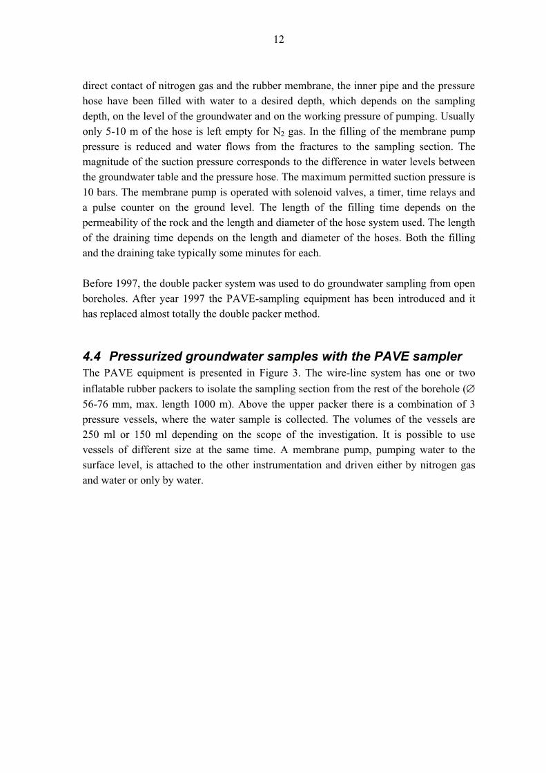
4.4 Pressurized groundwater samples with the PAVE sampler

The PAVE equipment is presented in Figure 3. The wire-line system has one or two

inflatable rubber packers to isolate the sampling section from the rest of the borehole (∅56-76 mm, max. length 1000 m). Above the upper packer there is a combination of 3

pressure vessels, where the water sample is collected. The volumes of the vessels are

250 ml or 150 ml depending on the scope of the investigation. It is possible to use

vessels of different size at the same time. A membrane pump, pumping water to the

surface level, is attached to the other instrumentation and driven either by nitrogen gas

and water or only by water.

13

Figure 3. The PAVE-equipment.

During the pumping period, groundwater is by-passing the pressure vessels. In this way,

microbial bio-films, drilling debris and other fine material will not accumulate on the

inner walls of the pressure vessels. Representativity of the groundwater is followed by

on-line measurements of pH, conductivity, Eh and dissolved oxygen. When the

parameters are stabilized and the water in the sampling section and in the hose has

changed at least three times, the sample for sodium fluorescine analysis can be taken. If

14

the concentration of the sodium fluorescine is less than 2 %, the sampling for field and

laboratory analyses is started. The sodium fluorescine level shows the amount drilling

water left in the sample.

As a final step of the sampling, the pressure vessels are filled with the groundwater

sample. Increase of hydraulic pressure in the pressure hose for the packers opens the

valve, which allows water flow through pressure vessels. As a result the argon or

nitrogen gas in the pressure compartment is compressed, the piston moves downwards,

and groundwater in situ-pressure fills to the sample compartment. Groundwater is

pumped through the pressure vessels for several hours in order get good quality samples.

Releasing the pressure in the pressure hose closes the valve and the PAVE equipment

together with the pressurized water samples is lifted to the surface level by using a

winch. The pressure vessels are shut and taken off from PAVE unit and sent to the

analysing laboratories.

Representativity of the data as been assessed in detail in Ruotsalainen et al. (2000). Most

influence to the results may have mixing of different bodies of groundwaters via

fractures, which can decrease or increase the EC values, depending on the salinities of

the in-mixed groundwaters. Other component is remaining drilling fluids which decrease

the EC values. These are analysed on basis of sodium fluorescine content. Apart of

mixing of waters, technical problems in the sampling equipment, e.g. leaking packers

can have some contribution by decreasing or increasing the EC values, depending on the

salinities of the in-mixed groundwaters. Finally, for hydrochemical investigations, the

uncertainties in analytical results, e.g. due to the heavy salt matrix of the groundwater

sample, may decreases or increase the salinity, if the contents of some of the main ions

(usually Ca) are uncertain. Features mentioned above may cause single difference

locations of the general trend, and from parallel other data.

4.5 Processing and control of the data quality

Groundwater samples from various depths from boreholes KR1-KR14 have been

collected and analyzed, and the results have been reported in OIVA-file (Palmén &

Hellä 2003). The extent of the analysis programme has varied between the samples.

When multiple analyses have been available, the most representative analysis has been

chosen to the model.

Water samples have been taken from the open boreholes and from double or

multipackered boreholes. In addition to the field measurements and analysis, the

laboratory tests have included determination of the Physico-chemical parameters, anions

and cations, isotopes, dissolved gases and particle fraction analysis.

15

In OIVA-file the results of the sampling and analyses have been summarized during the

over ten years of characterisation. It has been revised from the OL-PARVI file, which

was maintained by Fortum Power and Heat Oy until year 2000. All data from the earlier

PARVI-file is included in the present OIVA-file. All new results since the beginning of

the year 2001 have been archived to the OIVA-file.

The OIVA-file does not contain all groundwater chemistry measuring results measured

at Olkiluoto. Results of some samples have been removed from the files due to weak

representativity of the sampling. The OIVA-file is maintained, and the quality of the

results is controlled by Ms. Mia Mäntynen in Posiva Oy.

The quality control of the TDS analyses in OIVA-file is based on the charge balance

value CB:

CB = [Cations (mEq/l) – Anions (mEq/l)] / [Cations (mEq/l) + Anions (mEq/l)] * 100

(9)

Charge balance values < -5% and > 5% indicate uncertainty in chemical analysis. CB-

values were used to exclude uncertain TDS-values when multiple samples or analyses

were available from same location.

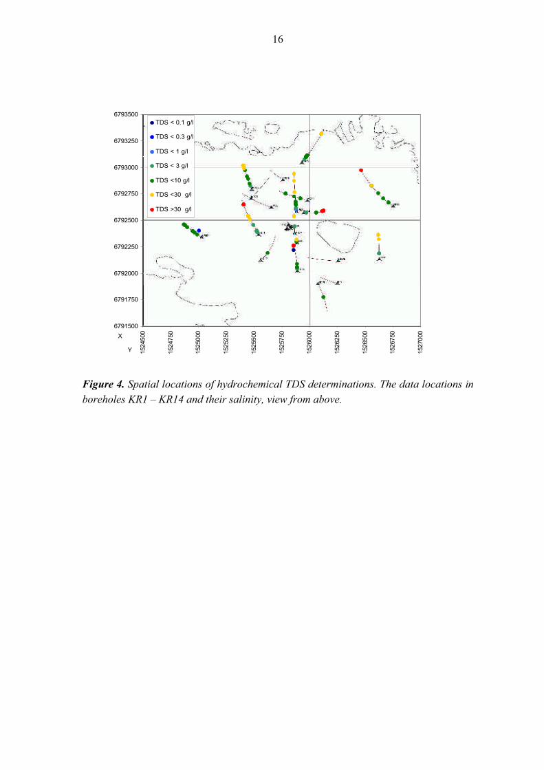
A total of 96 analyzed TDS-values from boreholes KR1-KR14 were used as a base of

the 3D groundwater salinity model. The measured electrical conductivities from 48

samples were recursively adjusted back to in situ temperatures using the flowmeter

temperatures. The location and salinity class of the data has been displayed in Figures 4

– 7.

16

6791500

6791750

6792000

6792250

6792500

6792750

6793000

6793250

6793500

1524500

1524750

1525000

1525250

1525500

1525750

1526000

1526250

1526500

1526750

1527000

Y

X

TDS < 0.1 g/l

TDS < 0.3 g/l

TDS < 1 g/l

TDS < 3 g/l

TDS <10 g/l

TDS <30 g/l

TDS >30 g/l

Figure 4. Spatial locations of hydrochemical TDS determinations. The data locations in

boreholes KR1 – KR14 and their salinity, view from above.

17

-980

-880

-780

-680

-580

-480

-380

-280

-180

-80

20

6791645

6791895

6792145

6792395

6792645

6792895

6793145

Y

Z

TDS < 0.1 g/l

TDS < 0.3 g/l

TDS < 1 g/l

TDS < 3 g/l

TDS <10 g/l

TDS <30 g/l

TDS >30 g/l

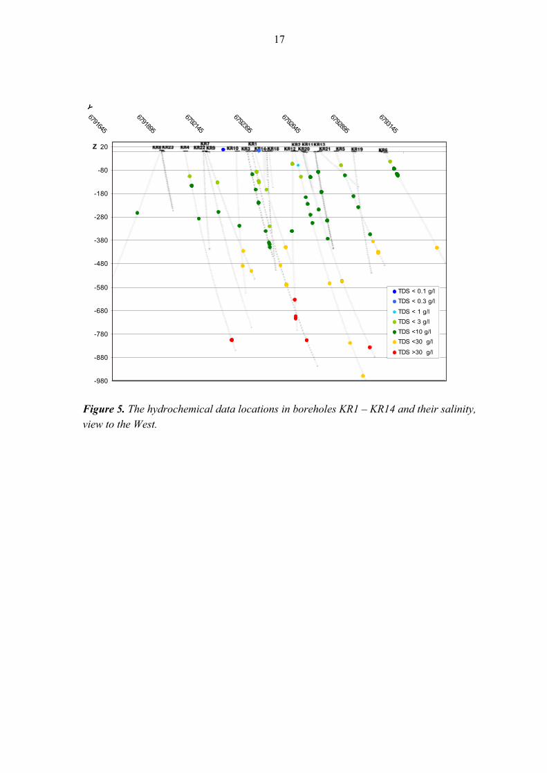
Figure 5. The hydrochemical data locations in boreholes KR1 – KR14 and their salinity,

view to the West.

18

-1000

-900

-800

-700

-600

-500

-400

-300

-200

-100

0

1524000

1524250

1524500

1524750

1525000

1525250

1525500

1525750

1526000

1526250

1526500

1526750

1527000

1527250

1527500

1527750

1528000

X

Z

TDS < 0.1 g/l

TDS < 0.3 g/l

TDS < 1 g/l

TDS < 3 g/l

TDS <10 g/l

TDS <30 g/l

TDS >30 g/l

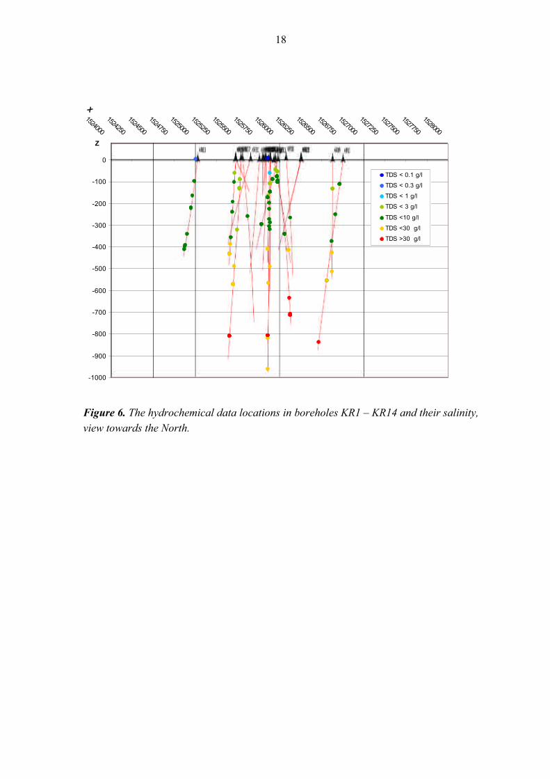
Figure 6. The hydrochemical data locations in boreholes KR1 – KR14 and their salinity,

view towards the North.

19

0

10

20

30

40

50

60

70

80

90

100

-1100-900-700-500-300-100

Vertical Depth, m

TD

S,

g/l

Hydrochemical TDS g/l

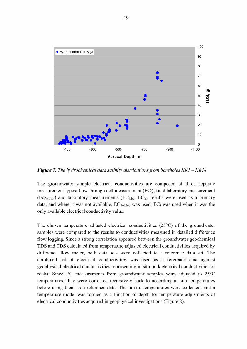
Figure 7. The hydrochemical data salinity distributions from boreholes KR1 – KR14.

The groundwater sample electrical conductivities are composed of three separate

measurement types: flow-through cell measurement (ECf), field laboratory measurement

(Ecfieldlab) and laboratory measurements (EClab). EClab results were used as a primary

data, and where it was not available, ECfieldlab was used. ECf was used when it was the

only available electrical conductivity value.

The chosen temperature adjusted electrical conductivities (25°C) of the groundwater

samples were compared to the results to conductivities measured in detailed difference

flow logging. Since a strong correlation appeared between the groundwater geochemical

TDS and TDS calculated from temperature adjusted electrical conductivities acquired by

difference flow meter, both data sets were collected to a reference data set. The

combined set of electrical conductivities was used as a reference data against

geophysical electrical conductivities representing in situ bulk electrical conductivities of

rocks. Since EC measurements from groundwater samples were adjusted to 25°Ctemperatures, they were corrected recursively back to according in situ temperatures

before using them as a reference data. The in situ temperatures were collected, and a

temperature model was formed as a function of depth for temperature adjustments of

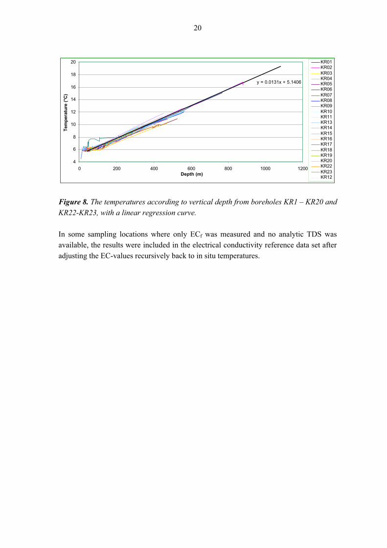
electrical conductivities acquired in geophysical investigations (Figure 8).

20

y = 0.0131x + 5.1406

4

6

8

10

12

14

16

18

20

0 200 400 600 800 1000 1200

Depth (m)

Tem

per

atu

re (

°C)

KR01KR02

KR03KR04KR05KR06

KR07KR08KR09

KR10KR11KR13KR14

KR15KR16KR17

KR18KR19KR20KR22

KR23KR12

Figure 8. The temperatures according to vertical depth from boreholes KR1 – KR20 and

KR22-KR23, with a linear regression curve.

In some sampling locations where only ECf was measured and no analytic TDS was

available, the results were included in the electrical conductivity reference data set after

adjusting the EC-values recursively back to in situ temperatures.

21

5 DIFFERENCE FLOW METER DATA

5.1 Description of the difference flow meter

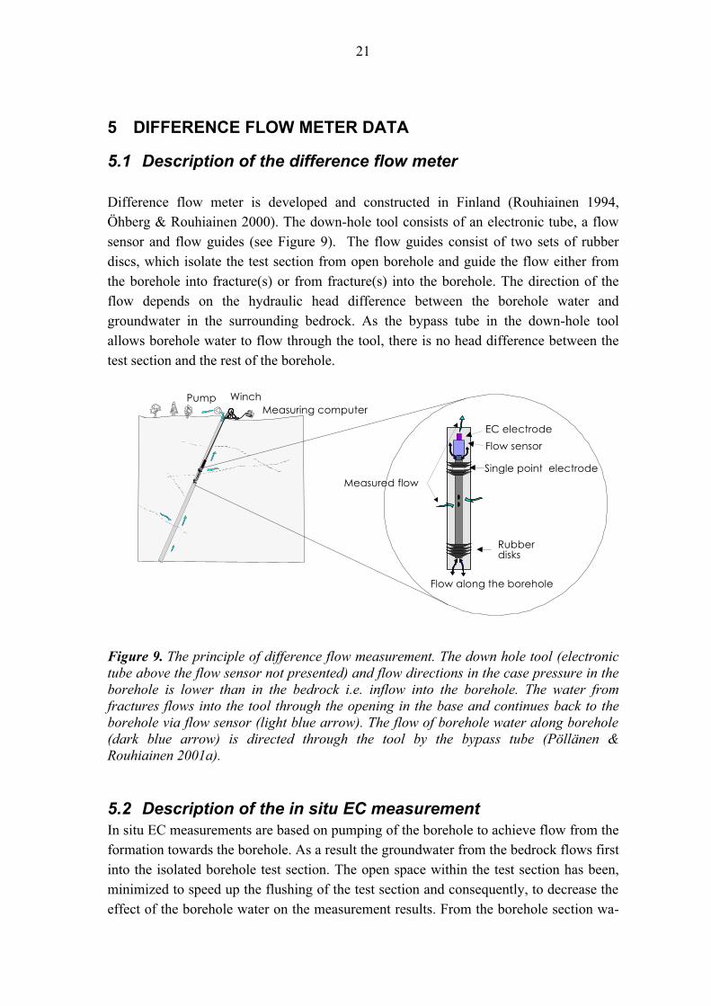
Difference flow meter is developed and constructed in Finland (Rouhiainen 1994,

Öhberg & Rouhiainen 2000). The down-hole tool consists of an electronic tube, a flow

sensor and flow guides (see Figure 9). The flow guides consist of two sets of rubber

discs, which isolate the test section from open borehole and guide the flow either from

the borehole into fracture(s) or from fracture(s) into the borehole. The direction of the

flow depends on the hydraulic head difference between the borehole water and

groundwater in the surrounding bedrock. As the bypass tube in the down-hole tool

allows borehole water to flow through the tool, there is no head difference between the

test section and the rest of the borehole.

WinchPumpMeasuring computer

Flow along the borehole

Rubberdisks

Flow sensor

Single point electrode

EC electrode

Measured flow

Figure 9. The principle of difference flow measurement. The down hole tool (electronic

tube above the flow sensor not presented) and flow directions in the case pressure in the

borehole is lower than in the bedrock i.e. inflow into the borehole. The water from

fractures flows into the tool through the opening in the base and continues back to the

borehole via flow sensor (light blue arrow). The flow of borehole water along borehole

(dark blue arrow) is directed through the tool by the bypass tube (Pöllänen &

Rouhiainen 2001a).

5.2 Description of the in situ EC measurement

In situ EC measurements are based on pumping of the borehole to achieve flow from the

formation towards the borehole. As a result the groundwater from the bedrock flows first

into the isolated borehole test section. The open space within the test section has been,

minimized to speed up the flushing of the test section and consequently, to decrease the

effect of the borehole water on the measurement results. From the borehole section wa-

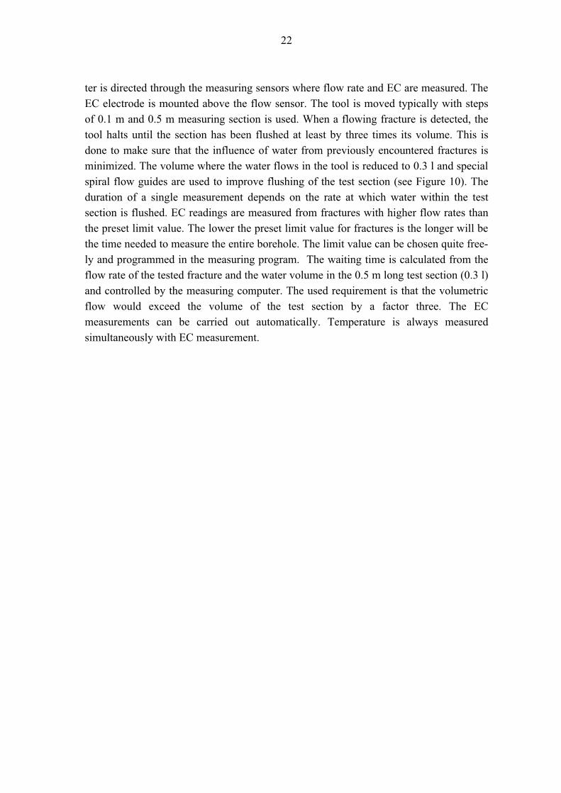
22

ter is directed through the measuring sensors where flow rate and EC are measured. The

EC electrode is mounted above the flow sensor. The tool is moved typically with steps

of 0.1 m and 0.5 m measuring section is used. When a flowing fracture is detected, the

tool halts until the section has been flushed at least by three times its volume. This is

done to make sure that the influence of water from previously encountered fractures is

minimized. The volume where the water flows in the tool is reduced to 0.3 l and special

spiral flow guides are used to improve flushing of the test section (see Figure 10). The

duration of a single measurement depends on the rate at which water within the test

section is flushed. EC readings are measured from fractures with higher flow rates than

the preset limit value. The lower the preset limit value for fractures is the longer will be

the time needed to measure the entire borehole. The limit value can be chosen quite free-

ly and programmed in the measuring program. The waiting time is calculated from the

flow rate of the tested fracture and the water volume in the 0.5 m long test section (0.3 l)

and controlled by the measuring computer. The used requirement is that the volumetric

flow would exceed the volume of the test section by a factor three. The EC

measurements can be carried out automatically. Temperature is always measured

simultaneously with EC measurement.

23

Figure 10. The detailed flow logging probe with the EC-electrode (TDS-electrode) and

the spiral (left).

5.3 Quality control of in situ EC-measurements

Two type of uncertainty has been found in measured results of in situ EC by difference

flow meter:

1. Flow guides are leaking in highly fractured sections enabling borehole water to

flow through the flow and EC sensors i.e. the EC-result does not necessarily

represent water from fractures at depth in question.

2. In situ EC has not been stabilized during the measurement i.e. there is an

increasing or decreasing trend at the end of the measurement.

24

Quality control for the first issue has not been done due to the difficulty to detect and

analyze the effect of possible leakage of flow guides, although time curves of in situ EC

values were analyzed visually and strong trend was found at eight depths in different

boreholes. Seven of trends were towards increasing salinity. In addition, the very high

single value (EC=17) at depth of 880 m (borehole length) in KR2 was assumed to be

caused by technical problem in the tool. On the other hand, some indications on very

high EC and density at the bottom part of borehole KR2 has been found and detailed

investigation are planned to find out the origin of such results.

There are factors in the measured EC values, which may influence to the representativity

of the results (Ruotsalainen et al. 2000). Amount of dissolved gases in the groundwater

may decrease the EC values as long as there are gas bubbles are present in the

groundwater. Remaining drilling fluids can decrease the EC values. For in situ EC

measurement these are not analysed. Other factors with influence can be technical

problems in the flowmeter, e.g. leaking flowguides, which can decrease or increase the

EC values, depending on the salinities of the in-mixed groundwaters, or prevent the

sampling from a fracture. Also the open hole effects (flow along the borehole) may

influence by decreasing or increasing the EC values, especially in locations where flow

from open borehole has been into the bedrock. And finally the pumping during the EC

measurement increases the EC values, because of up flow of saline water in open

borehole. The details mentioned above may occur as deviations from general trends, or

differences in parallel data from same locations. On the other hand, differences may well

indicate also variation in natural conditions.

5.4 Reference data

The temperature adjusted electrical conductivities measured from groundwater samples

were used as a reference data for conductivities measured in detailed difference flow

logging. Since a strong correlation between the Groundwater geochemical conductivities

and difference flow meter conductivities appeared, the data sets were combined to form

a reference data set for geophysical resistivity data.

5.5 Processing of the data

The last measurement of each EC-series of detailed difference flow logging

measurement series was collected from boreholes KR1-KR20, KR22 and KR23.

Acquired values were adjusted to represent apparent TDS (using conductivity in 25°C

temperature) according to formulas and procedures described in Posiva Working report

2002-10 (Heikkonen et al. 2002). Old results where standard water conductivity

25

calculation procedure (SFS 1994) had been applied, were also corrected (Heikkinen et

al. 1996, Ruotsalainen et al. 2000).

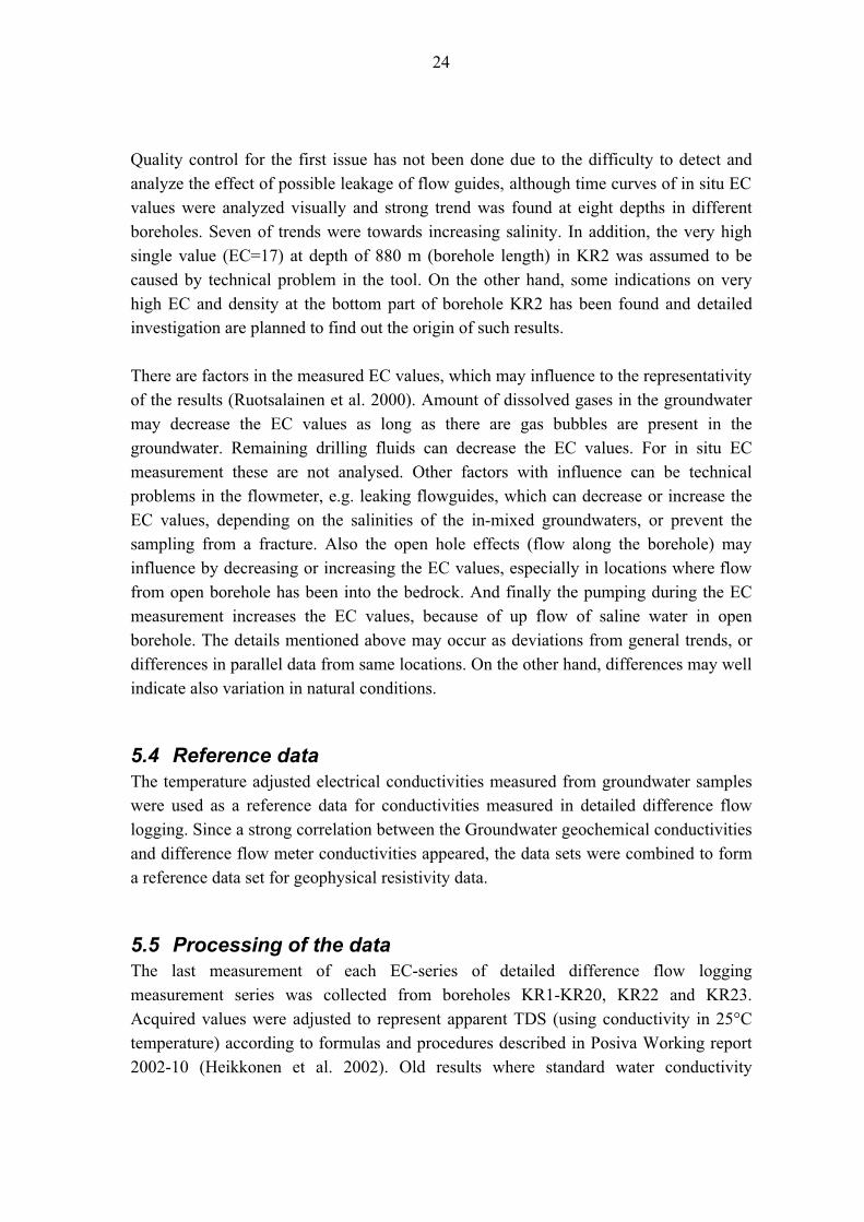
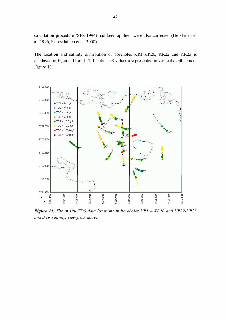
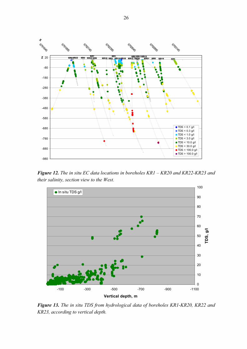
The location and salinity distribution of boreholes KR1-KR20, KR22 and KR23 is

displayed in Figures 11 and 12. In situ TDS values are presented in vertical depth axis in

Figure 13.

6791500

6791750

6792000

6792250

6792500

6792750

6793000

6793250

6793500

1524500

1524750

1525000

1525250

1525500

1525750

1526000

1526250

1526500

1526750

1527000

Y

X

TDS < 0.1 g/l

TDS < 0.3 g/l

TDS < 1.0 g/l

TDS < 3.0 g/l

TDS < 10.0 g/l

TDS < 30.0 g/l

TDS < 100.0 g/l

TDS > 100.0 g/l

Figure 11. The in situ TDS data locations in boreholes KR1 – KR20 and KR22-KR23

and their salinity, view from above.

26

-980

-880

-780

-680

-580

-480

-380

-280

-180

-80

20

6791645

6791895

6792145

6792395

6792645

6792895

6793145

X

Z

TDS < 0.1 g/l

TDS < 0.3 g/l

TDS < 1.0 g/l

TDS < 3.0 g/l

TDS < 10.0 g/l

TDS < 30.0 g/l

TDS < 100.0 g/l

TDS > 100.0 g/l

Figure 12. The in situ EC data locations in boreholes KR1 – KR20 and KR22-KR23 and

their salinity, section view to the West.

0

10

20

30

40

50

60

70

80

90

100

-1100-900-700-500-300-100

Vertical depth, m

TD

S,

g/l

In situ TDS g/l

Figure 13. The in situ TDS from hydrological data of boreholes KR1-KR20, KR22 and

KR23, according to vertical depth.

27

5.6 Comparison of in situ data to hydrochemical data

Hydrochemical TDS values according to depth were presented in Figure 7 (Chapter

4.5,), and in situ TDS in Figure 13. Figure 14 displays both of the data for comparison.

Hydrochemical data is shown as single TDS value over a packer interval (at least 2 m,

often tens of meters for mid point of each interval). The TDS computed from in situ EC

data is assigned to a single fracture thus representing a confined depth value in

centimeter accuracy. Often there are several in situ TDS values for each hydrochemical

sample value location.

This becomes simply from a fact that there are several flowing fractures at the specific

depth level. Quite naturally, there have also occurred differences between the

observations with different methods. Sometimes in a section the individual fractures

display an increasing trend according to depth. In some other cases there are differences

in the results obtained different times. These differences have been discussed and

displayed for boreholes KR1 – KR11 in report (Ruotsalainen et al. 2000), and were not

reproduced for this report. Assessment did not cover extended parts of KR6, KR7 and

KR8, nor boreholes KR12 – KR14, or later re-investigations in these boreholes.

Possible reasons for differences can be considered being:

1) Fractures at the sections have natural differences in TDS, e.g., change in

salinity level or dilution of salinity in fracture zones containing open

fractures; more closed fractures may contain more saline water etc.

2) The hydrochemical investigation is averaging the TDS obtained from all

fractures; typically also the water is obtained from the best flowing

fractures at the section; while in situ EC can distinguish between several

fractures

3) Open borehole flow has intruded fresh water into some of the fractures;

situation has not yet stabilized for in situ EC measurement

4) Pumping during hydrological measurement (in situ EC) has brought in

more saline water from deeper parts of borehole, the bedrock along the

fractures but also along open borehole which may disturb measured

results

5) Pumping during hydrochemical sampling has brought in less saline water

from upper part of the borehole especially along open borehole above the

upper packer

Both in situ EC and hydrochemical TDS definitions suffer from difficulties to obtain

water from deeper parts of the bedrock. Fractures are more scarce and closed, pumping

more difficult.

Possible variations in the measurement techniques and applications will influence to the

representativity of the method. Most probable is, that the method specific differences are

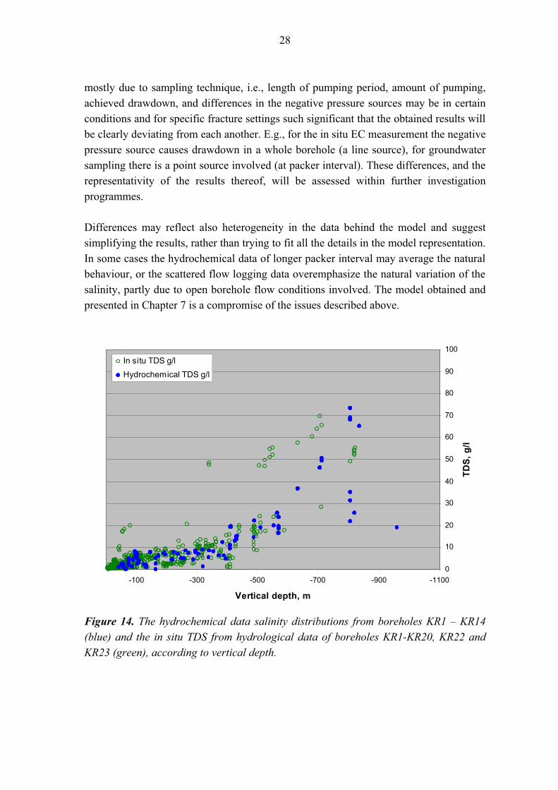
28

mostly due to sampling technique, i.e., length of pumping period, amount of pumping,

achieved drawdown, and differences in the negative pressure sources may be in certain

conditions and for specific fracture settings such significant that the obtained results will

be clearly deviating from each another. E.g., for the in situ EC measurement the negative

pressure source causes drawdown in a whole borehole (a line source), for groundwater

sampling there is a point source involved (at packer interval). These differences, and the

representativity of the results thereof, will be assessed within further investigation

programmes.

Differences may reflect also heterogeneity in the data behind the model and suggest

simplifying the results, rather than trying to fit all the details in the model representation.

In some cases the hydrochemical data of longer packer interval may average the natural

behaviour, or the scattered flow logging data overemphasize the natural variation of the

salinity, partly due to open borehole flow conditions involved. The model obtained and

presented in Chapter 7 is a compromise of the issues described above.

0

10

20

30

40

50

60

70

80

90

100

-1100-900-700-500-300-100

Vertical depth, m

TD

S,

g/l

In situ TDS g/l

Hydrochemical TDS g/l

Figure 14. The hydrochemical data salinity distributions from boreholes KR1 – KR14

(blue) and the in situ TDS from hydrological data of boreholes KR1-KR20, KR22 and

KR23 (green), according to vertical depth.

29

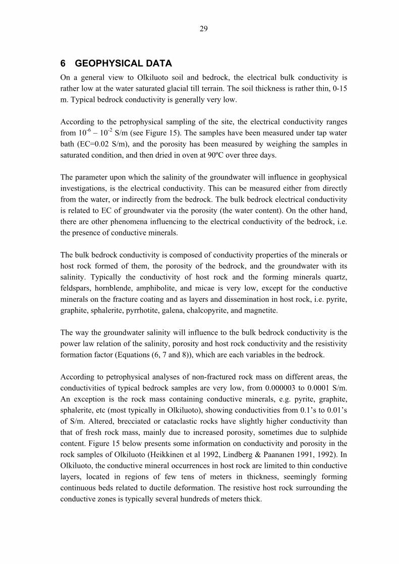
6 GEOPHYSICAL DATA

On a general view to Olkiluoto soil and bedrock, the electrical bulk conductivity is

rather low at the water saturated glacial till terrain. The soil thickness is rather thin, 0-15

m. Typical bedrock conductivity is generally very low.

According to the petrophysical sampling of the site, the electrical conductivity ranges

from 10-6 – 10-2 S/m (see Figure 15). The samples have been measured under tap water

bath (EC=0.02 S/m), and the porosity has been measured by weighing the samples in

saturated condition, and then dried in oven at 90ºC over three days.

The parameter upon which the salinity of the groundwater will influence in geophysical

investigations, is the electrical conductivity. This can be measured either from directly

from the water, or indirectly from the bedrock. The bulk bedrock electrical conductivity

is related to EC of groundwater via the porosity (the water content). On the other hand,

there are other phenomena influencing to the electrical conductivity of the bedrock, i.e.

the presence of conductive minerals.

The bulk bedrock conductivity is composed of conductivity properties of the minerals or

host rock formed of them, the porosity of the bedrock, and the groundwater with its

salinity. Typically the conductivity of host rock and the forming minerals quartz,

feldspars, hornblende, amphibolite, and micae is very low, except for the conductive

minerals on the fracture coating and as layers and dissemination in host rock, i.e. pyrite,

graphite, sphalerite, pyrrhotite, galena, chalcopyrite, and magnetite.

The way the groundwater salinity will influence to the bulk bedrock conductivity is the

power law relation of the salinity, porosity and host rock conductivity and the resistivity

formation factor (Equations (6, 7 and 8)), which are each variables in the bedrock.

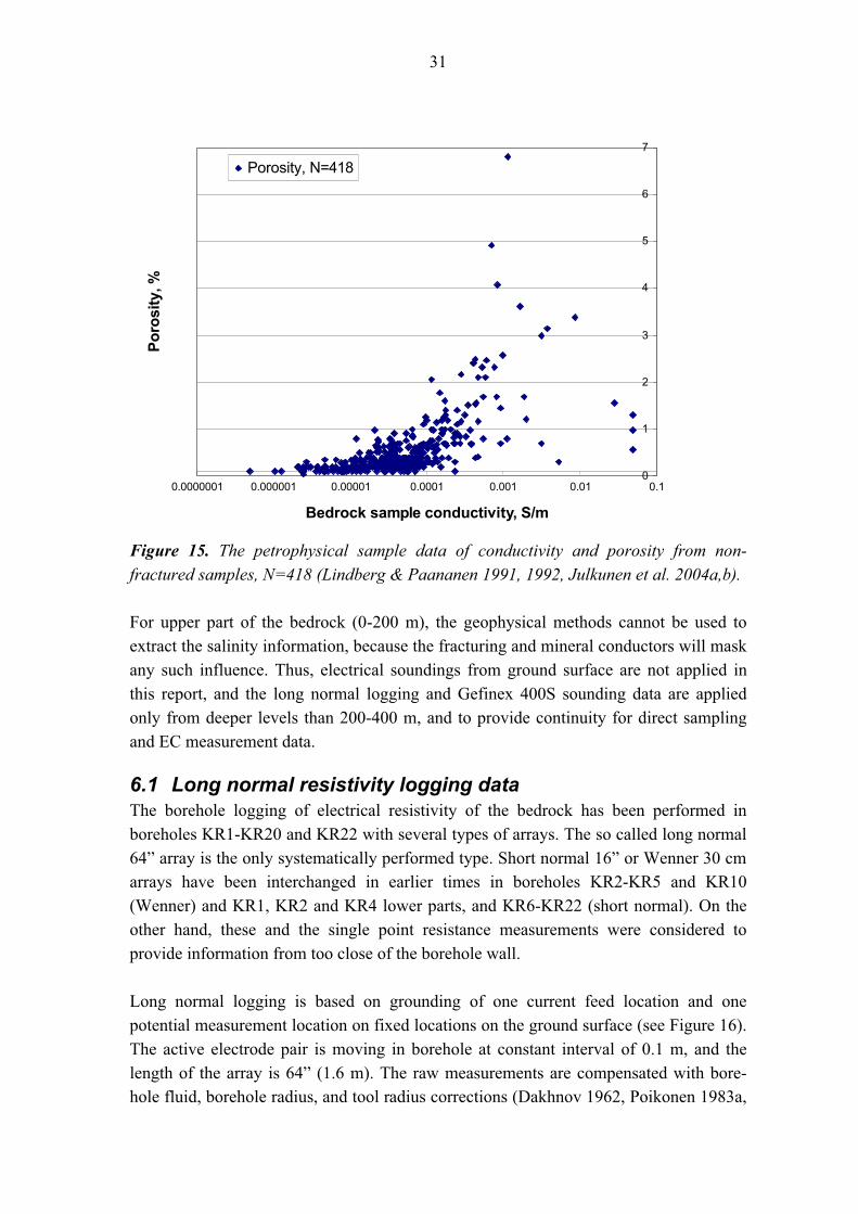
According to petrophysical analyses of non-fractured rock mass on different areas, the

conductivities of typical bedrock samples are very low, from 0.000003 to 0.0001 S/m.

An exception is the rock mass containing conductive minerals, e.g. pyrite, graphite,

sphalerite, etc (most typically in Olkiluoto), showing conductivities from 0.1’s to 0.01’s

of S/m. Altered, brecciated or cataclastic rocks have slightly higher conductivity than

that of fresh rock mass, mainly due to increased porosity, sometimes due to sulphide

content. Figure 15 below presents some information on conductivity and porosity in the

rock samples of Olkiluoto (Heikkinen et al 1992, Lindberg & Paananen 1991, 1992). In

Olkiluoto, the conductive mineral occurrences in host rock are limited to thin conductive

layers, located in regions of few tens of meters in thickness, seemingly forming

continuous beds related to ductile deformation. The resistive host rock surrounding the

conductive zones is typically several hundreds of meters thick.

30

Conductivity of groundwater in Olkiluoto has ranged from 0.01 S/m for fresh surface

waters, to 1-10 S/m for deep seated fluids below 400-500 m depth. The porosity is low,

in fresh host rock mostly less than 0.5%, ranging 0.2 – 6.8% in non fractured

(microfractured) rock containing no conductive minerals. Up to 4% porosity the

dependency of resistivity and porosity is nearly linear. Porosity is in narrow fracture

zones locally exceeding 5%, on basis of apparent porosities calculated from acoustic

logging (Okko et al. 1990). Fracture frequency ranges in sparsely fractured rock mass

from 1-3 pcs/m. The definition of fracture zone implies the frequency would exceed 10

pcs/m at limited volumes (7-8% of borehole length) (Vaittinen et al. 2003).

The bulk conductivity (measured as its inverse, resistivity) of the bedrock mass has been

investigated with geophysical logging, using short 16” and long 64” normal, and in some

boreholes 30 cm Wenner arrays, in scale of few tens of metres to some metres. Apparent

conductivity ranges in sparsely fractured, weakly conductive rock at 0.0001 – 0.00002

S/m. In fracture zones the apparent conductivities are 0.2 – 0.0005 S/m, and even higher

when conductive minerals are coating the fracture surfaces. The conductive regions

display conductivities of 2 – 0.05 S/m at narrow limited zones (Heikkinen et al. 1992,

Okko et al. 1990; references listed in Table 1).

The soil types are commonly clacial till, saturated with water and covered typically with

some peat. The fine fraction (silt and clay layered in sea bottom) will increase the

conductivity of the soil. Bedrock is outcropping in several locations. Typical non-

saturated conductivity of the soil ranges from 0.001 – 0.0005 S/m. For peat the

conductivity is 0.02 – 0.5 S/m. Water saturated layer of the till can display conductivities

from 0.01 to 0.002 S/m. The uppermost 100-150 m of the bedrock displays higher

frequency of fractures, and thus also higher conductivity in bedrock (0.001 – 0.0001 S/m

when there’s no presence of mineral conductors). The uppermost few metres of bedrock

under the soil may be strongly weathered in several places.

The characteristic increased fracturing at the surface part, thus the higher water content,

will increase the electrical conductivity. Although in the upper part of the bedrock the

presence and infiltration of marine brackish water may occur, it cannot be distinguished

on basis of geophysical investigations. Character of the in situ bedrock conductivity

distribution, along with the open borehole and fracture in situ groundwater EC values

from same depth ranges, are displayed in Appendix 3 (boreholes KR1, KR2, KR4, KR7,

KR9, KR11, KR12, KR19). In these boreholes the trend visible from 400-500 m level

downwards was assessed to represent increasing salinity in the bedrock. These values

were used to assess the bedrock groundwater salinity. Data is shown in Figures 19-21,

and the process to obtain TDS data in Chapter 6.1.

31

0

1

2

3

4

5

6

7

0.0000001 0.000001 0.00001 0.0001 0.001 0.01 0.1

Bedrock sample conductivity, S/m

Po

rosi

ty, %

Porosity, N=418

Figure 15. The petrophysical sample data of conductivity and porosity from non-

fractured samples, N=418 (Lindberg & Paananen 1991, 1992, Julkunen et al. 2004a,b).

For upper part of the bedrock (0-200 m), the geophysical methods cannot be used to

extract the salinity information, because the fracturing and mineral conductors will mask

any such influence. Thus, electrical soundings from ground surface are not applied in

this report, and the long normal logging and Gefinex 400S sounding data are applied

only from deeper levels than 200-400 m, and to provide continuity for direct sampling

and EC measurement data.

6.1 Long normal resistivity logging data

The borehole logging of electrical resistivity of the bedrock has been performed in

boreholes KR1-KR20 and KR22 with several types of arrays. The so called long normal

64” array is the only systematically performed type. Short normal 16” or Wenner 30 cm

arrays have been interchanged in earlier times in boreholes KR2-KR5 and KR10

(Wenner) and KR1, KR2 and KR4 lower parts, and KR6-KR22 (short normal). On the

other hand, these and the single point resistance measurements were considered to

provide information from too close of the borehole wall.

Long normal logging is based on grounding of one current feed location and one

potential measurement location on fixed locations on the ground surface (see Figure 16).

The active electrode pair is moving in borehole at constant interval of 0.1 m, and the

length of the array is 64” (1.6 m). The raw measurements are compensated with bore-

hole fluid, borehole radius, and tool radius corrections (Dakhnov 1962, Poikonen 1983a,

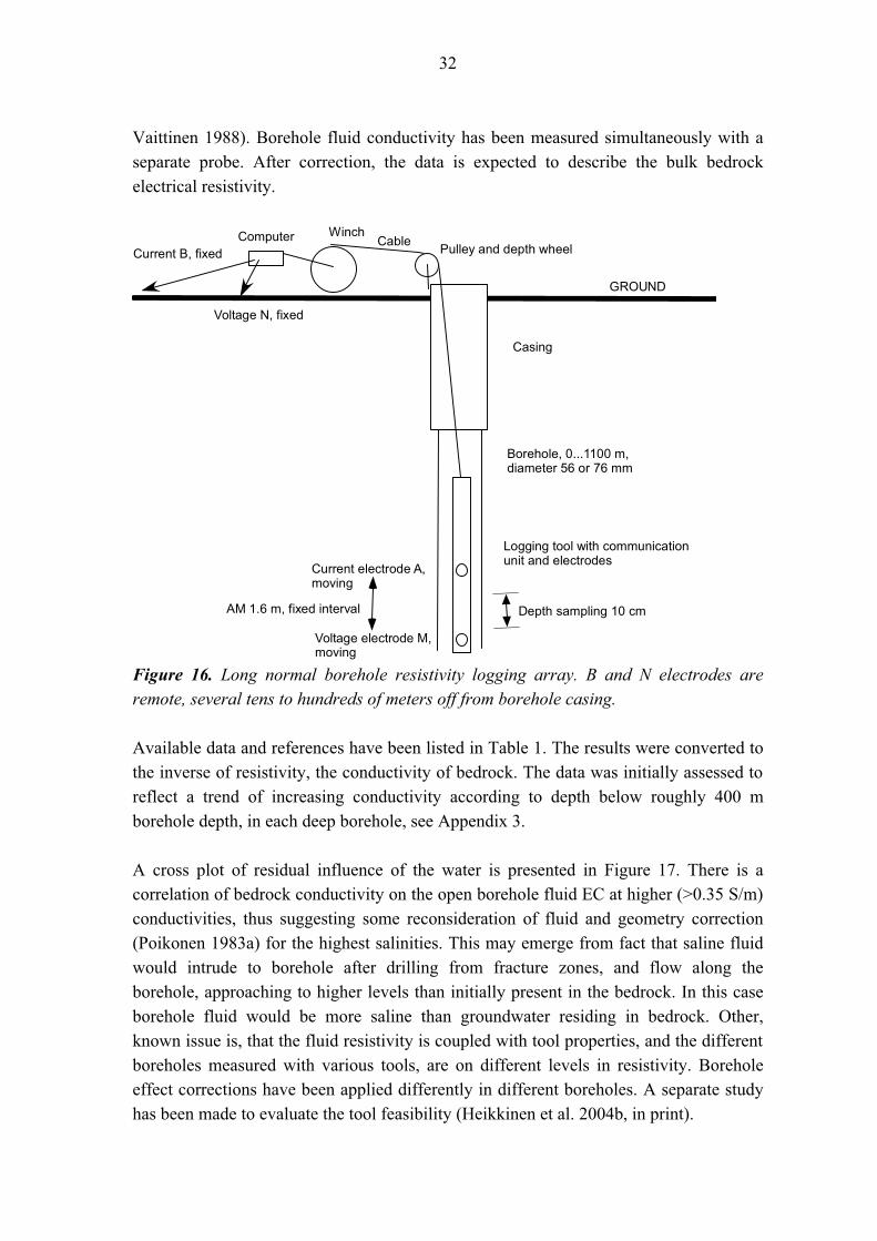
32

Vaittinen 1988). Borehole fluid conductivity has been measured simultaneously with a

separate probe. After correction, the data is expected to describe the bulk bedrock

electrical resistivity.

Borehole, 0...1100 m,diameter 56 or 76 mm

CableComputer Winch

Pulley and depth wheel

Casing

Logging tool with communicationunit and electrodes

Current electrode A,moving

Voltage electrode M,moving

AM 1.6 m, fixed interval Depth sampling 10 cm

GROUND

Current B, fixed

Voltage N, fixed

Figure 16. Long normal borehole resistivity logging array. B and N electrodes are

remote, several tens to hundreds of meters off from borehole casing.

Available data and references have been listed in Table 1. The results were converted to

the inverse of resistivity, the conductivity of bedrock. The data was initially assessed to

reflect a trend of increasing conductivity according to depth below roughly 400 m

borehole depth, in each deep borehole, see Appendix 3.

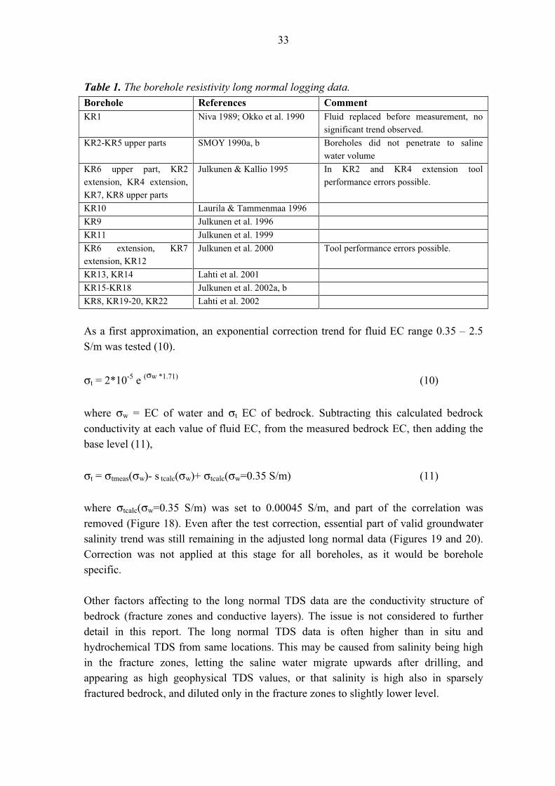
A cross plot of residual influence of the water is presented in Figure 17. There is a

correlation of bedrock conductivity on the open borehole fluid EC at higher (>0.35 S/m)

conductivities, thus suggesting some reconsideration of fluid and geometry correction

(Poikonen 1983a) for the highest salinities. This may emerge from fact that saline fluid

would intrude to borehole after drilling from fracture zones, and flow along the

borehole, approaching to higher levels than initially present in the bedrock. In this case

borehole fluid would be more saline than groundwater residing in bedrock. Other,

known issue is, that the fluid resistivity is coupled with tool properties, and the different

boreholes measured with various tools, are on different levels in resistivity. Borehole

effect corrections have been applied differently in different boreholes. A separate study

has been made to evaluate the tool feasibility (Heikkinen et al. 2004b, in print).

33

Table 1. The borehole resistivity long normal logging data.

Borehole References Comment

KR1 Niva 1989; Okko et al. 1990 Fluid replaced before measurement, no

significant trend observed.

KR2-KR5 upper parts SMOY 1990a, b Boreholes did not penetrate to saline

water volume

KR6 upper part, KR2

extension, KR4 extension,

KR7, KR8 upper parts

Julkunen & Kallio 1995 In KR2 and KR4 extension tool

performance errors possible.

KR10 Laurila & Tammenmaa 1996

KR9 Julkunen et al. 1996

KR11 Julkunen et al. 1999

KR6 extension, KR7

extension, KR12

Julkunen et al. 2000 Tool performance errors possible.

KR13, KR14 Lahti et al. 2001

KR15-KR18 Julkunen et al. 2002a, b

KR8, KR19-20, KR22 Lahti et al. 2002

As a first approximation, an exponential correction trend for fluid EC range 0.35 – 2.5

S/m was tested (10).

σt = 2*10-5 e (σw *1.71) (10)

where σw = EC of water and σt EC of bedrock. Subtracting this calculated bedrock

conductivity at each value of fluid EC, from the measured bedrock EC, then adding the

base level (11),

σt = σtmeas(σw)- s tcalc(σw)+ σtcalc(σw=0.35 S/m) (11)

where σtcalc(σw=0.35 S/m) was set to 0.00045 S/m, and part of the correlation was

removed (Figure 18). Even after the test correction, essential part of valid groundwater

salinity trend was still remaining in the adjusted long normal data (Figures 19 and 20).

Correction was not applied at this stage for all boreholes, as it would be borehole

specific.

Other factors affecting to the long normal TDS data are the conductivity structure of

bedrock (fracture zones and conductive layers). The issue is not considered to further

detail in this report. The long normal TDS data is often higher than in situ and

hydrochemical TDS from same locations. This may be caused from salinity being high

in the fracture zones, letting the saline water migrate upwards after drilling, and

appearing as high geophysical TDS values, or that salinity is high also in sparsely

fractured bedrock, and diluted only in the fracture zones to slightly lower level.

34

0.00001

0.0001

0.001

0.01

0.1

1

0.01 0.1 1 10

Fluid conductivity, S/m

Bed

rock

co

nd

uct

ivit

y, S

/m

LN Cond

Figure 17. Groundwater conductivity and bedrock apparent conductivity, KR19.

y = 2E-05e1.7107x

0.00001

0.0001

0.001

0.01

0.1

1

0.1 1 10

EC (borehole fluid), S/m

EC

(lo

ng

no

rmal

), S

/m

LN Cond High

LN

LN FIT

CORRECTED

Expon. (LN)

Figure 18. Fitted function between groundwater and bedrock EC. The high EC(long

normal) values are from conductive mineral containing layers, and from fracture zones.

35

0.000001

0.00001

0.0001

0.001

0.01

0.1

1

0 100 200 300 400 500 600

Depth, m

Bed

rock

EC

, S/m

0.001

0.01

0.1

1

10

100

1000

Bo

reh

ole

flu

id E

C, S

/m

LN Conductivity LNConductivity_adj Fluid conductivity S/m

Figure 19. Adjusted bedrock EC and groundwater EC. Adjustment fits well the lowest

conductivities (sparsely fractured, non conductive rock) but will leave the fracture zones

untouched. The adjustment does not fit well at low conductivity fluid conditions (<0.35

S/m), where the Poikonen’s (1983a) and Dakhnov’s (1962) formula is known to be valid

for the applied tools.

36

0.00001

0.0001

0.001

0.01

0.1

1

0.01 0.1 1 10

EC (borehole water), S/m

EC

(lo

ng

no

rmal

ad

just

ed),

S/m

LNCond_adj

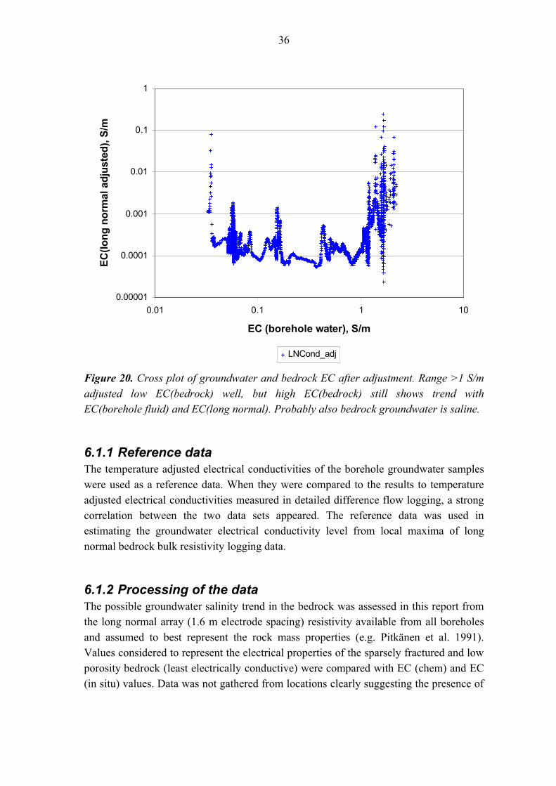
Figure 20. Cross plot of groundwater and bedrock EC after adjustment. Range >1 S/m

adjusted low EC(bedrock) well, but high EC(bedrock) still shows trend with

EC(borehole fluid) and EC(long normal). Probably also bedrock groundwater is saline.

6.1.1 Reference data

The temperature adjusted electrical conductivities of the borehole groundwater samples

were used as a reference data. When they were compared to the results to temperature

adjusted electrical conductivities measured in detailed difference flow logging, a strong

correlation between the two data sets appeared. The reference data was used in

estimating the groundwater electrical conductivity level from local maxima of long

normal bedrock bulk resistivity logging data.

6.1.2 Processing of the data

The possible groundwater salinity trend in the bedrock was assessed in this report from

the long normal array (1.6 m electrode spacing) resistivity available from all boreholes

and assumed to best represent the rock mass properties (e.g. Pitkänen et al. 1991).

Values considered to represent the electrical properties of the sparsely fractured and low

porosity bedrock (least electrically conductive) were compared with EC (chem) and EC

(in situ) values. Data was not gathered from locations clearly suggesting the presence of

37

graphite or sulphides, or from strongly fractured sections, where resistivity variation is

caused by other factors than groundwater salinity.

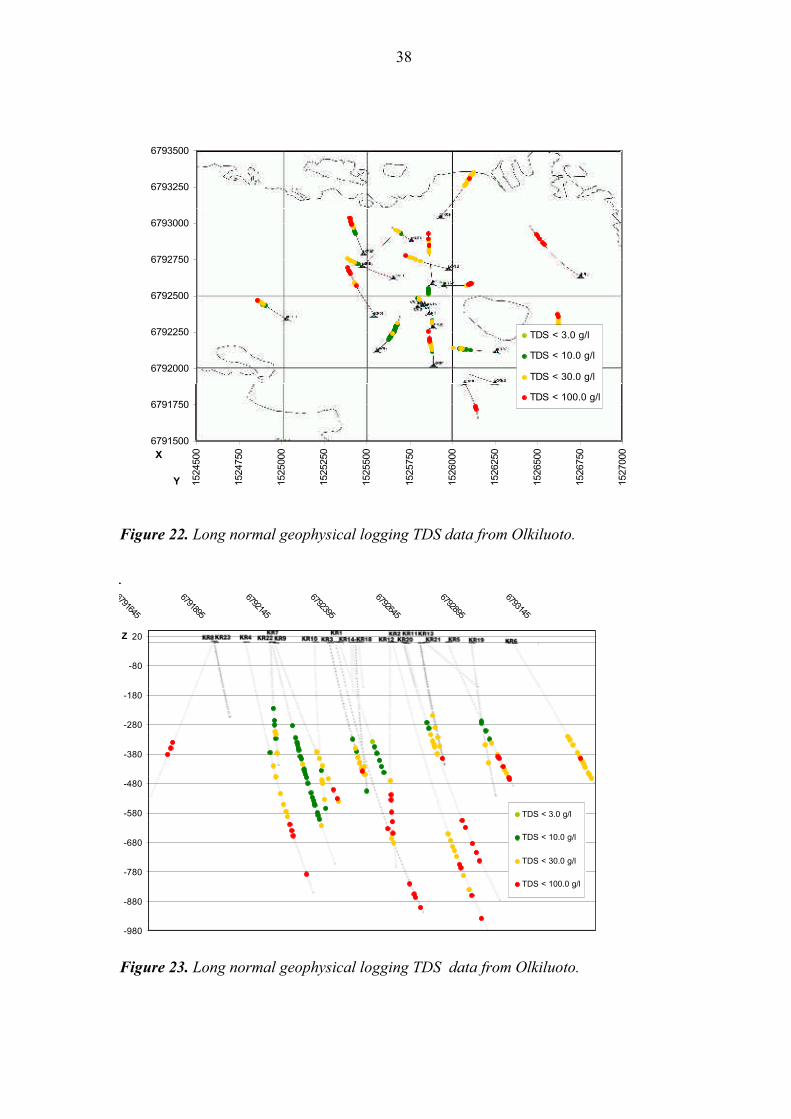
The results have been displayed in Figures 21 – 23. The results have been shown also in

Appendix 4 in a spatial view, showing also the model layer boundaries defined from

hydrochemical TDS and in situ EC data. The general coincidence of downwards

increasing salinity is realistic. When comparing the long normal logging derived TDS

data to the model, it can be observed that the logging data would exaggerate TDS, and

suggest the boundary of highest salinity to be at upper level in bedrock. Also the data

from upper layers would display slightly too a high salinity. This is probably both due to

inadequate compensation for open borehole saline water in preceding processing, the

tool and borehole specific differences in long normal measurements, and due to

difficulty in defining an accurate EC to TDS conversion ratio for bedrock electrical

conductivity. More precise way to correlate these issues would be to define the porosity

and formation factor of the bedrock, perhaps together with density or NMR, or acoustic

measurements, and then to use the Long Normal resistivity or other applicable downhole

tool (e.g. Laterolog) to define the true bulk resistivity and that way the pore water

salinity.

0

10

20

30

40

50

60

70

80

-1100-900-700-500-300-100

Vertical depth, m

TD

S, g

/l

Long normal TDS (calc.)

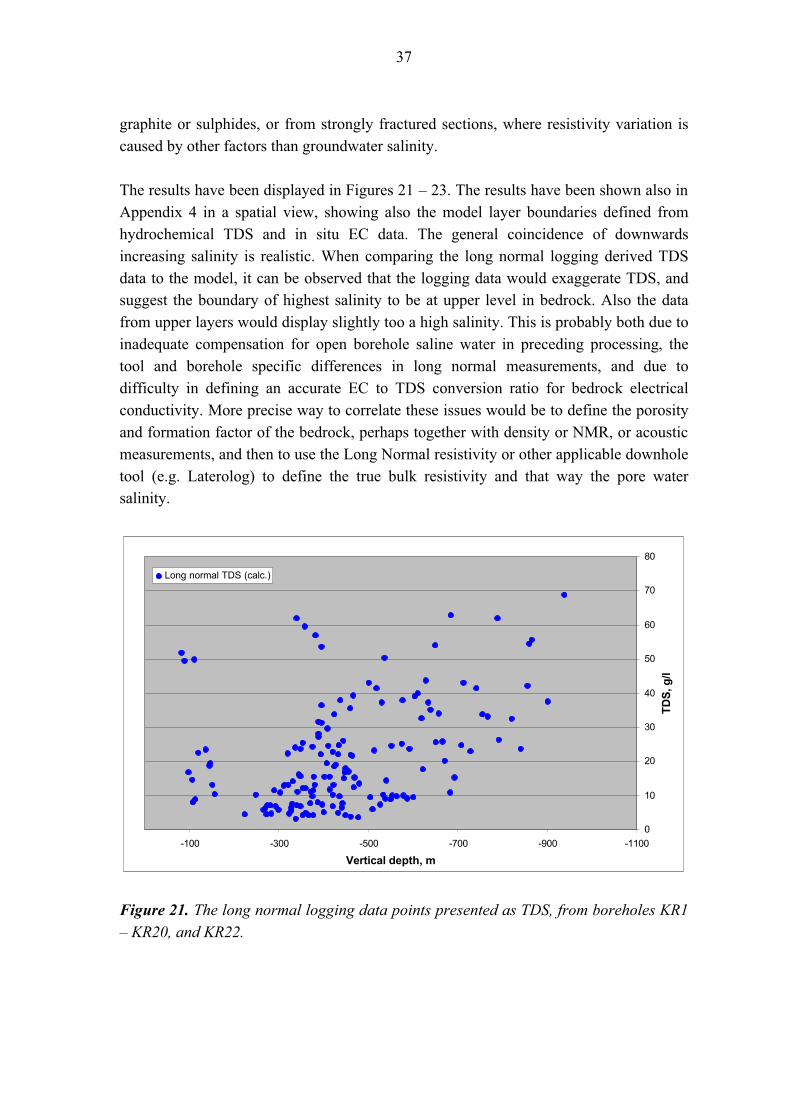
Figure 21. The long normal logging data points presented as TDS, from boreholes KR1

– KR20, and KR22.

38

6791500

6791750

6792000

6792250

6792500

6792750

6793000

6793250

6793500

1524500

1524750

1525000

1525250

1525500

1525750

1526000

1526250

1526500

1526750

1527000

Y

X

TDS < 3.0 g/l

TDS < 10.0 g/l

TDS < 30.0 g/l

TDS < 100.0 g/l

Figure 22. Long normal geophysical logging TDS data from Olkiluoto.

-980

-880

-780

-680

-580

-480

-380

-280

-180

-80

20

6791645

6791895

6792145

6792395

6792645

6792895

6793145

X

Z

TDS < 3.0 g/l

TDS < 10.0 g/l

TDS < 30.0 g/l

TDS < 100.0 g/l

Figure 23. Long normal geophysical logging TDS data from Olkiluoto.

39

6.2 GEOPHYSICAL ELECTROMAGNETIC GEFINEX 400S DATA

The frequency domain electromagnetic Gefinex 400 S sounding method has been

applied several times at Olkiluoto site, mainly for mapping of the saline groundwater.

Soundings were conducted during years 1990 and 1994 (Paananen et al. 1991, Jokinen

& Jokinen 1994) and in 2002 (Ahokas 2003).

6.2.1 The GEFINEX 400S method

The Gefinex 400S (Sampo) is a wide-band electromagnetic sounding system designed

by Outokumpu Group. The method is used for determining inductively the electrical

resistivity of the subsurface at different depths. The method is based on vertical

magnetic dipole field at wide frequency range, introduced with a electrical current loop,

and measurement of magnetic field vertical Hz and horizontal Hx and Hy components

(real and imaginary parts) and their relative phase angles. A total of 81 discrete

frequencies can be measured between 2.3 Hz and 19840 Hz (20 frequencies per decade).

The basic measurable, ratio Hx/Hz, is recorded for each frequency.

The transmitter consists of an electronic unit, a power control unit, transmitter cables

(either a 20 m diameter circular loop or a 50 m x 50 m square loop) and re-chargeable

batteries. The receiver consists of an electronics unit and an antenna (three coils

measuring the vertical and two horizontal components of the EM field). The

configuration of the Gefinex 400S equipment is presented in Figure 24.

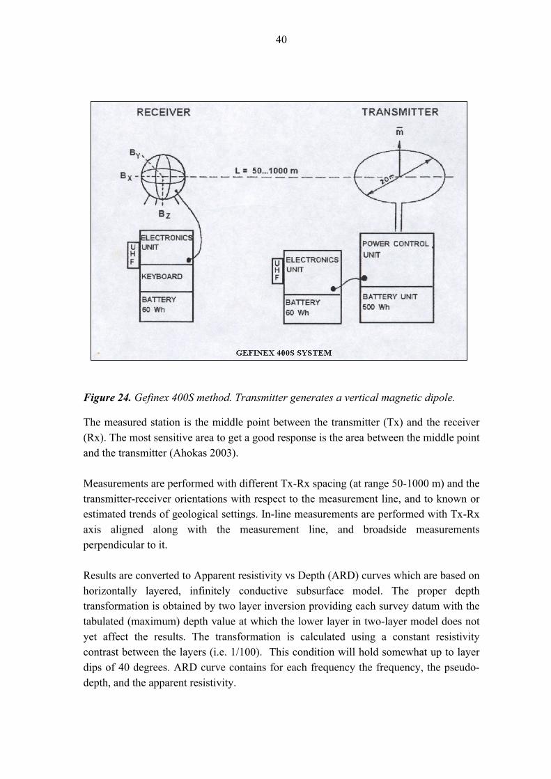
40

Figure 24. Gefinex 400S method. Transmitter generates a vertical magnetic dipole.

The measured station is the middle point between the transmitter (Tx) and the receiver

(Rx). The most sensitive area to get a good response is the area between the middle point

and the transmitter (Ahokas 2003).

Measurements are performed with different Tx-Rx spacing (at range 50-1000 m) and the

transmitter-receiver orientations with respect to the measurement line, and to known or

estimated trends of geological settings. In-line measurements are performed with Tx-Rx

axis aligned along with the measurement line, and broadside measurements

perpendicular to it.

Results are converted to Apparent resistivity vs Depth (ARD) curves which are based on

horizontally layered, infinitely conductive subsurface model. The proper depth

transformation is obtained by two layer inversion providing each survey datum with the

tabulated (maximum) depth value at which the lower layer in two-layer model does not

yet affect the results. The transformation is calculated using a constant resistivity

contrast between the layers (i.e. 1/100). This condition will hold somewhat up to layer

dips of 40 degrees. ARD curve contains for each frequency the frequency, the pseudo-

depth, and the apparent resistivity.

41

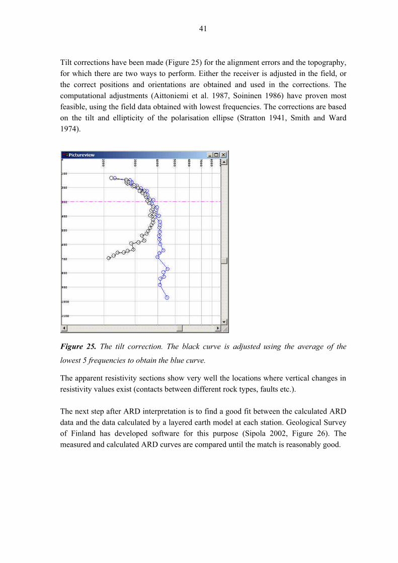
Tilt corrections have been made (Figure 25) for the alignment errors and the topography,

for which there are two ways to perform. Either the receiver is adjusted in the field, or

the correct positions and orientations are obtained and used in the corrections. The

computational adjustments (Aittoniemi et al. 1987, Soininen 1986) have proven most

feasible, using the field data obtained with lowest frequencies. The corrections are based

on the tilt and ellipticity of the polarisation ellipse (Stratton 1941, Smith and Ward

1974).

Figure 25. The tilt correction. The black curve is adjusted using the average of the

lowest 5 frequencies to obtain the blue curve.

The apparent resistivity sections show very well the locations where vertical changes in

resistivity values exist (contacts between different rock types, faults etc.).

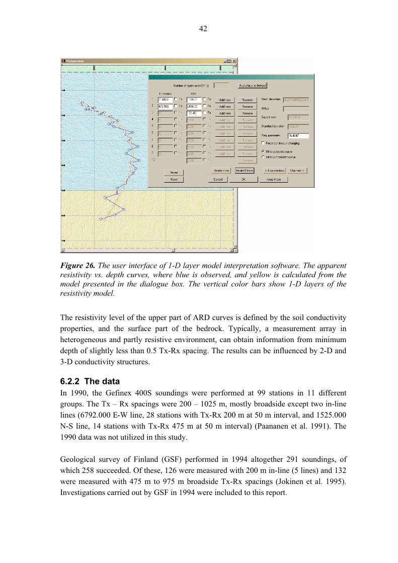
The next step after ARD interpretation is to find a good fit between the calculated ARD

data and the data calculated by a layered earth model at each station. Geological Survey

of Finland has developed software for this purpose (Sipola 2002, Figure 26). The

measured and calculated ARD curves are compared until the match is reasonably good.

42

Figure 26. The user interface of 1-D layer model interpretation software. The apparent

resistivity vs. depth curves, where blue is observed, and yellow is calculated from the

model presented in the dialogue box. The vertical color bars show 1-D layers of the

resistivity model.

The resistivity level of the upper part of ARD curves is defined by the soil conductivity

properties, and the surface part of the bedrock. Typically, a measurement array in

heterogeneous and partly resistive environment, can obtain information from minimum

depth of slightly less than 0.5 Tx-Rx spacing. The results can be influenced by 2-D and

3-D conductivity structures.

6.2.2 The dataIn 1990, the Gefinex 400S soundings were performed at 99 stations in 11 different

groups. The Tx – Rx spacings were 200 – 1025 m, mostly broadside except two in-line

lines (6792.000 E-W line, 28 stations with Tx-Rx 200 m at 50 m interval, and 1525.000

N-S line, 14 stations with Tx-Rx 475 m at 50 m interval) (Paananen et al. 1991). The

1990 data was not utilized in this study.

Geological survey of Finland (GSF) performed in 1994 altogether 291 soundings, of

which 258 succeeded. Of these, 126 were measured with 200 m in-line (5 lines) and 132

were measured with 475 m to 975 m broadside Tx-Rx spacings (Jokinen et al. 1995).

Investigations carried out by GSF in 1994 were included to this report.

43

Suomen Malmi Oy conducted supplementary electromagnetic frequency soundings with

Gefinex 400S equipment for Posiva Oy for studying the subsurface resistivity structures

at Olkiluoto site during autumn 2002 (Ahokas 2003). The surveys were carried out both

with in-line and broadside configurations with coil separations of 200m, 500 m and 800

m. The soundings were conducted at one line where totally 197 stations were measured;

73 stations by a coil separation of 200 m using broadside coil configuration, 71 stations

by a coil separation of 200 m using in-line configurations, 33 stations by a coil

separation of 500 m using broadside configuration and 10 stations by a coil separation of

800 m using broadside configuration.

The results are presented as tilt corrected apparent resistivity versus depth (ARD)

profiles, ARD profiles for different coil configurations, ellipticity profiles, tilt profiles as

well as ARD profiles from raw data and without tilt correction.

Original task was to apply the 1-D model resistivities and layer boundaries and

thicknesses in a straightforward manner in a similar way as in 1996 modelling. With

more dense measurements and reference data, detailedness of layer models was not

adequate for salinity interpretation. Models consist of representing thin higher

conductivity pyrite and graphite layers. The resistive, thicker layers between them

contain influence of the saline water, but are assigned with a single resistivity value.

More detailed layer model would be useful (Turo Ahokas, personal communication

27.10.2003). It has to be borne in mind that these results imply electrical equivalence

(the conductance of a layer can be given, not the thickness or conductivity separately

without using geometrical constrains).

It was decided to survey the ARD curves to extract general information on the apparent

conductivity variation. The ARD results altogether were plotted on the Excel, and their

location assessed. Any curves representing a trend of increasing salinity were adopted to

further analysis. Others, either too noisy or displaying potential 3-D effects, were

rejected. There was observed that the resistivity level in general is higher in the east part

of the site, and lower in the west part of the site. Probably this is due to the conductivity

heterogeneities in the upper part of bedrock.

Separate interpretation reports for bedrock conductive regions have been presented in

(Jokinen et al. 1995) and (Heikkinen et al. 2004a).

6.2.3 Quality control of the Gefinex 400S data

The quality control of the Gefinex 400S data sets was based on evaluations of ARD-

curves by Mr. Jokinen (Jokinen & Jokinen 1994), Mr. Turo Ahokas (Ahokas 2003).

Further exclusions of incoherent ARD-curves and outliers were performed by Mr. Jorma

Palmén.

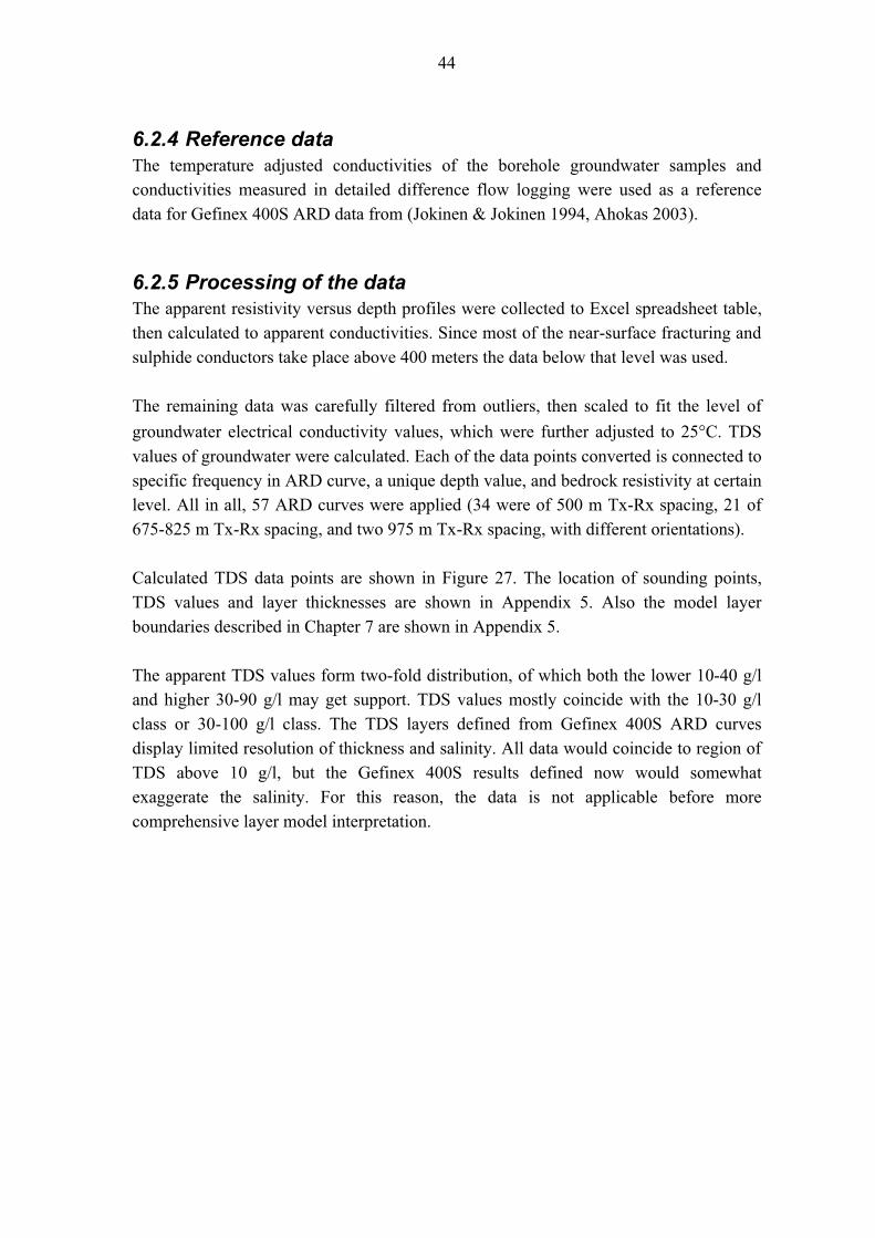
44

6.2.4 Reference data

The temperature adjusted conductivities of the borehole groundwater samples and

conductivities measured in detailed difference flow logging were used as a reference

data for Gefinex 400S ARD data from (Jokinen & Jokinen 1994, Ahokas 2003).

6.2.5 Processing of the data

The apparent resistivity versus depth profiles were collected to Excel spreadsheet table,

then calculated to apparent conductivities. Since most of the near-surface fracturing and

sulphide conductors take place above 400 meters the data below that level was used.

The remaining data was carefully filtered from outliers, then scaled to fit the level of

groundwater electrical conductivity values, which were further adjusted to 25°C. TDS

values of groundwater were calculated. Each of the data points converted is connected to

specific frequency in ARD curve, a unique depth value, and bedrock resistivity at certain

level. All in all, 57 ARD curves were applied (34 were of 500 m Tx-Rx spacing, 21 of

675-825 m Tx-Rx spacing, and two 975 m Tx-Rx spacing, with different orientations).

Calculated TDS data points are shown in Figure 27. The location of sounding points,

TDS values and layer thicknesses are shown in Appendix 5. Also the model layer

boundaries described in Chapter 7 are shown in Appendix 5.

The apparent TDS values form two-fold distribution, of which both the lower 10-40 g/l

and higher 30-90 g/l may get support. TDS values mostly coincide with the 10-30 g/l

class or 30-100 g/l class. The TDS layers defined from Gefinex 400S ARD curves

display limited resolution of thickness and salinity. All data would coincide to region of

TDS above 10 g/l, but the Gefinex 400S results defined now would somewhat

exaggerate the salinity. For this reason, the data is not applicable before more

comprehensive layer model interpretation.

45

0

20

40

60

80

100

120

140

-1100-900-700-500-300-100

Vertical depth, m

TD

S, g

/l

500 m coil separation1994

800 m coil separation 1994

975 m coil separation1994

500 m coil separation 2002

800 m coil separation 2002

Figure 27. The Gefinex 400S TDS data from Olkiluoto. The locations of data have been

presented in Appendix 5.

Using the TDS assessment based on geophysical data implied some features which may

need to taken into account. The resistivity of bedrock will depend both on porosity and

groundwater salinity, some assumptions on porosity in host rock and fractures need to be

made. In a large volume, a fairly uniform distribution of porosity has been assumed. The

presence of electrically conductive minerals has been taken into account with rejecting

data displaying a too high EC. Logging data has the same limitations on open borehole

flow conditions as the in situ EC has; and the borehole fluid salinity influence was

necessary to compensate from the results. For TDS calculation from the bedrock EC, the

properly selected reference points were essential. These points are quite few available.

Finally, the electromagnetic layer interpretations now concentrated to produce an

overview of the site, would get significant use of new interpretations with a consistent

geometrical model, higher number of layers, electrically conductive horizons clearly

separated from salinity responses, frequency dependency of EC encountered, and

electrical conductance equivalence of layer thickness and conductivity product taken

into account. In this work these points were treated in tentative manner. The details

listed above are the most probable reasons for the differences between hydrochemical

and in situ TDS compared to geophysical data.

46

47

7 3D SALINITY MODEL

To visualize the observed variation of salinity content of the groundwater a three-

dimensional salinity model description was compiled. The model covers the planned

repository volume, where deep boreholes are located. The limiting coordinates are

6791500 - 6793500 Northing and 1524500 - 1527000 Easting to a depth of -1000 m.

The earlier version of volumetric model of fluid salinity variation is described in

Heikkinen et al. (1996). At that time there was not enough hydrochemical data to create

a conceptual model of TDS salinity. For that reason, geophysical data was used as a

primary data for modelling. The model was rather complicated indicating very

heterogeneous conditions of salinity variation. After that first model, the number of

boreholes and groundwater investigations has increased significantly enabling the use of

direct observations. Although heterogeneity is still visible, a layered occurrence of

increasing salinity can be approximated. The model is compiled using simple layers and

focus has been to visualize the observations in 3D presentations.

Four different kinds of investigation data were available for model compilation: TDS

values calculated from the analytical results of the hydrochemical studies, TDS values

calculated from the in situ EC data of difference flow measurements, TDS values

calculated from the long normal resistivity logging data, and TDS values calculated from

the electromagnetic soundings. In case of long normal logging data the measured

resistivity results were disturbed due to salinity of open borehole water.

The determined TDS salinities based on hydrochemical data and in situ EC data are

presented in Figure 28 and Figure 29 respectively. For the detailed study, the salinity

values are classified to eight categories. In the modelling a rougher approach is used.

The salinity values are modelled with following boundary values: TDS less than 1 g/l

representing fresh water, TDS between 1 and 10 g/l representing brackish water, and

saline waters TDS above 10 g/l. The determined boundary surfaces follow above-

mentioned limit values forming three volumes.

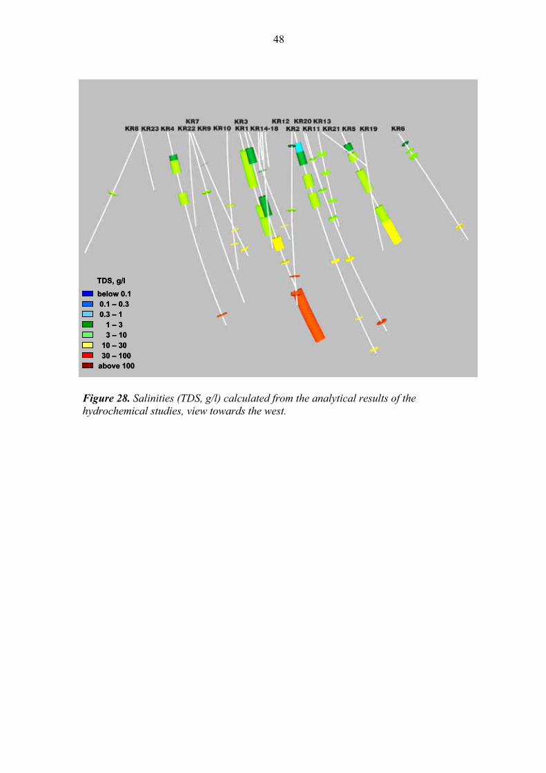
48

TDS, g/l

below 0.10.1 – 0.30.3 – 1

1 – 33 – 10

10 – 3030 – 100

above 100

TDS, g/l

below 0.10.1 – 0.30.3 – 1

1 – 33 – 10

10 – 3030 – 100

above 100

TDS, g/l

below 0.10.1 – 0.30.3 – 1

1 – 33 – 10

10 – 3030 – 100

above 100

Figure 28. Salinities (TDS, g/l) calculated from the analytical results of the

hydrochemical studies, view towards the west.

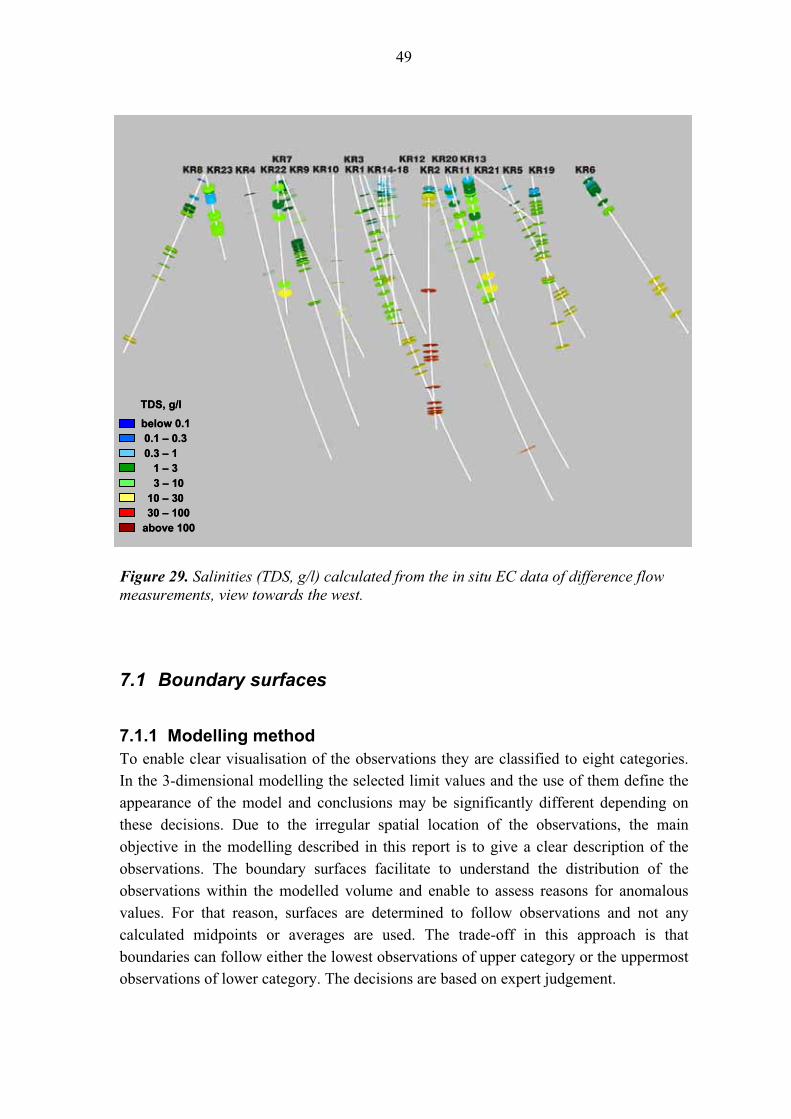
49

TDS, g/l

below 0.10.1 – 0.30.3 – 1

1 – 33 – 10

10 – 3030 – 100

above 100

TDS, g/l

below 0.10.1 – 0.30.3 – 1

1 – 33 – 10

10 – 3030 – 100

above 100

TDS, g/l

below 0.10.1 – 0.30.3 – 1

1 – 33 – 10

10 – 3030 – 100

above 100

Figure 29. Salinities (TDS, g/l) calculated from the in situ EC data of difference flow

measurements, view towards the west.

7.1 Boundary surfaces

7.1.1 Modelling methodTo enable clear visualisation of the observations they are classified to eight categories.

In the 3-dimensional modelling the selected limit values and the use of them define the

appearance of the model and conclusions may be significantly different depending on

these decisions. Due to the irregular spatial location of the observations, the main

objective in the modelling described in this report is to give a clear description of the

observations. The boundary surfaces facilitate to understand the distribution of the

observations within the modelled volume and enable to assess reasons for anomalous

values. For that reason, surfaces are determined to follow observations and not any

calculated midpoints or averages are used. The trade-off in this approach is that

boundaries can follow either the lowest observations of upper category or the uppermost

observations of lower category. The decisions are based on expert judgement.

50

The boundary surfaces are created using following method: selected observations points

are picked up, a surface is modelled based on triangulation of the observation points, the

average orientation of the surface is calculated, and finally the surface is extrapolated to

the limiting coordinates using the average orientation. The triangulation of the surfaces

is presented in Figure 30.

In the description of the boundary surfaces, the hydrochemical data and the in situ EC

data are shown separated to modelling categories. Created boundary surfaces are also

visualized.

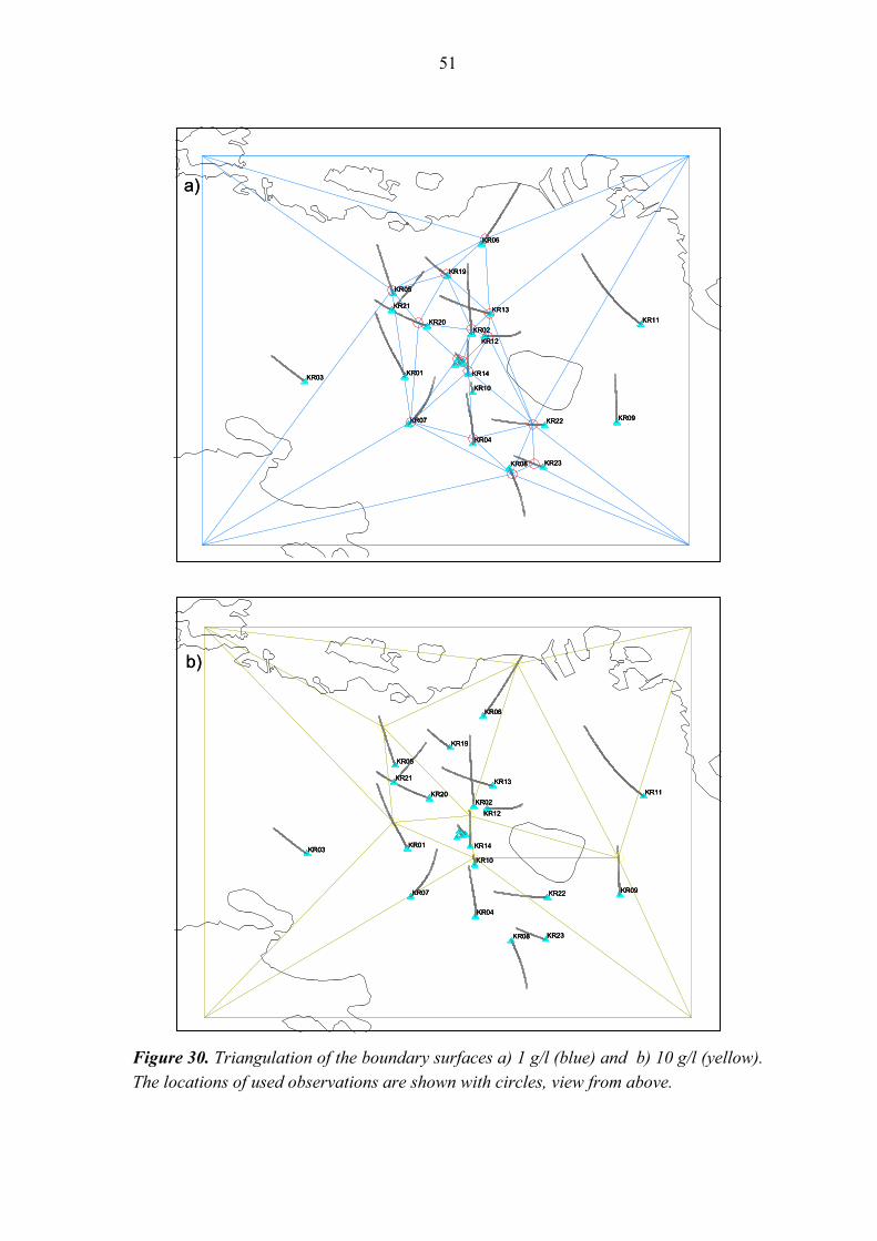
51

a)

b)

a)

b)

Figure 30. Triangulation of the boundary surfaces a) 1 g/l (blue) and b) 10 g/l (yellow).

The locations of used observations are shown with circles, view from above.

52

7.1.2 Boundary surface, TDS 1 g/lThe determination of the upper boundary surface is based on the in situ EC observations.

This surface follows the lowest observations of TDS values below 1 g/l (see Figure 31b),

except in two boreholes. Salinity value 0.84 g/l is determined at the borehole length

152.7 m in borehole KR1. In borehole KR6 at the borehole lengths 127.95 m, 128.35 m,

and 135.55 m, salinity values 0.94 - 0.95 g/l are determined. The boundary surface is

determined using TDS values from 15 boreholes, visualized in Figure 30a.

Although TDS values below 1 g/l form rather continuous horizontal layer, the in situ

TDS values belonging to category 1 - 3 g/l are commonly measured above the boundary

surface of 1 g/l. Altogether in nine boreholes observations are mixed, see Figure 32b.

Two of the hydrochemical samples are partly located above the upper surface. The

sample, taken in borehole KR2, belong to this category and the other one taken in

borehole KR4 belong to the category 1 - 3 g/l, see Figure 31a.

The orientation of the boundary surface is sub-horizontal (146º/2º). The depth values of

the observations used for the surface range from -5 m in borehole KR13 to -103 m in

borehole KR4 (Figure 31b).

7.1.3 Boundary surface, TDS 10 g/lThe lower boundary surface is determined on the basis of the hydrochemical

observations following the uppermost observations of the values above 10 g/l. The

salinity values are classified to categories 1 - 3 g/l and 3 - 10 g/l, but the Figure 32a and

Figure 32b show that these categories do not occur as sequential layered formation.

Using this boundary surface also the in situ EC TDS values 1 - 10 g/l are mostly located

above the surface (Figure 32a and Figure 32b). Only in borehole KR1, values of the

category 1 - 10 g/l are observed below the boundary surface, see Figure 32b. At the

borehole lengths of 525.97 m and 537.89 m values 8.6 g/l and 9.2 g/l are obtained.

Several fractures are located in this region, each with slightly different in situ EC,

mainly increasing according to the depth. This may indicate either dilution of fracture

water with borehole water, or natural transition of salinity level in a local fracture zone.

The boundary surface 10 g/l is determined based on six observations (Figure 30b) of

hydrochemical data. It can be seen in Figure 33b that in situ EC data TDS values 10 - 30

g/l are more scattered covering the depth section -250 - -550 m, while the hydrochemical

observations are all located below -400 m.

During the in situ EC measurement of borehole KR12 (Figure 34b), pumping of the

borehole has raised the saline groundwater from a fracture at borehole length 744.8 m

53

along the borehole and possibly in the bedrock too (up-coning) (Pöllänen & Rouhiainen

2001) and the results between -350 - -600 m are uncertain.

The orientation of the boundary surface is sub-horizontal (191º/3º). The depth values of

the observations used for the surface range from -386 m in borehole KR5 to -487 m in

borehole KR10 (Figure 33a).

So far, the highest TDS value of the Olkiluoto site is based on in situ EC measurements,

105.5 g/l, and it has been obtained from borehole KR2 at the depth of 880.24 - 880.74

m. However, there are also five other in situ EC measurements between the depths

878.88 - 880.24 m, which TDS salinities range from 52.22 to 55.48 g/l. TDS salinities of

borehole KR2 vary also in hydrochemical studies. At the depth sections, 876.0 - 881.0 m

and 1030.0 - 1038 m TDS values of 25.7 g/l and 19.1 g/l are measured, but when the

open borehole was measured with tube sampling tool (Ruotsalainen et al. 2000,

Ruotsalainen & Alhonmäki-Aalonen 1996), approximately 75 g/l was observed from the

bottom section 1000 - 1050 m. Presently, hydrochemical studies are continued in

borehole KR2 and indications of high TDS values are obtained.

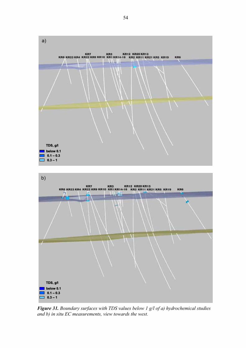
54

TDS, g/l

below 0.10.1 – 0.30.3 – 1

TDS, g/l

below 0.10.1 – 0.30.3 – 1

a)

b)

TDS, g/l

below 0.10.1 – 0.30.3 – 1

TDS, g/l

below 0.10.1 – 0.30.3 – 1

TDS, g/l

below 0.10.1 – 0.30.3 – 1

TDS, g/l

below 0.10.1 – 0.30.3 – 1

TDS, g/l

below 0.10.1 – 0.30.3 – 1

TDS, g/l

below 0.10.1 – 0.30.3 – 1

a)

b)

Figure 31. Boundary surfaces with TDS values below 1 g/l of a) hydrochemical studies

and b) in situ EC measurements, view towards the west.

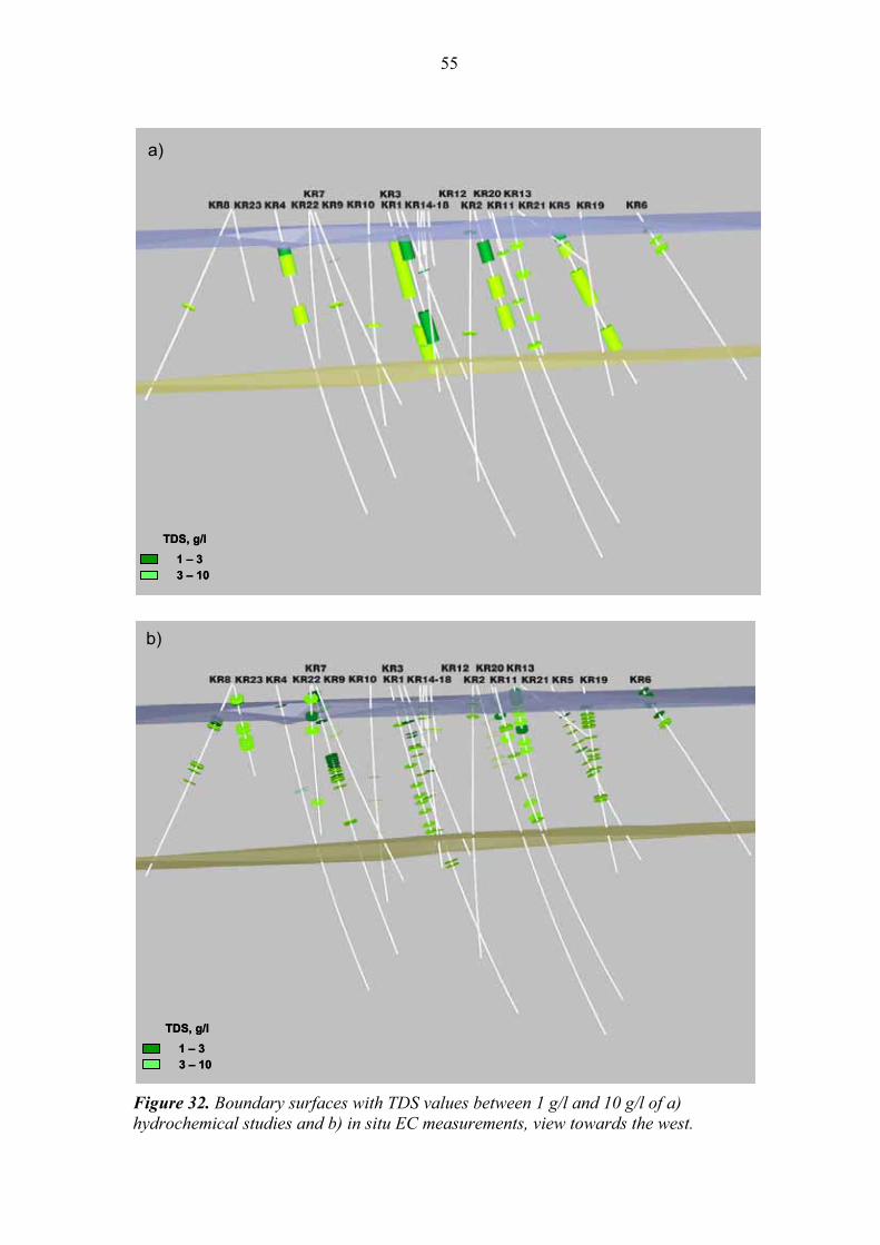
55

TDS, g/l

1 – 33 – 10

TDS, g/l

1 – 33 – 10

a)

b)

TDS, g/l

1 – 33 – 10

TDS, g/l

1 – 33 – 10

TDS, g/l

1 – 33 – 10

TDS, g/l

1 – 33 – 10

TDS, g/l

1 – 33 – 10

TDS, g/l

1 – 33 – 10

a)

b)

Figure 32. Boundary surfaces with TDS values between 1 g/l and 10 g/l of a)

hydrochemical studies and b) in situ EC measurements, view towards the west.

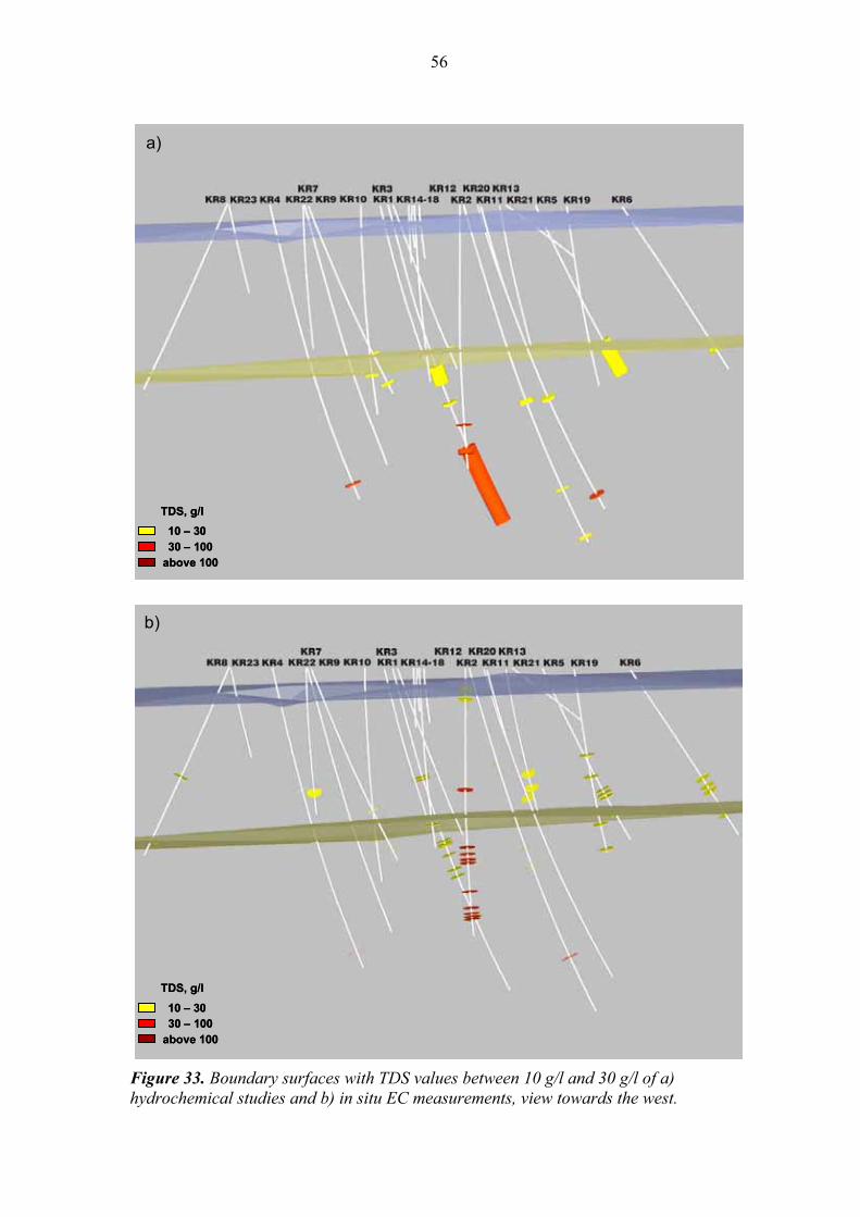
56

TDS, g/l

10 – 3030 – 100

above 100

TDS, g/l

10 – 3030 – 100

above 100

a)

b)

TDS, g/l

10 – 3030 – 100

above 100

TDS, g/l

10 – 3030 – 100

above 100

TDS, g/l

10 – 3030 – 100

above 100

TDS, g/l

10 – 3030 – 100

above 100

TDS, g/l

10 – 3030 – 100

above 100

a)

b)

Figure 33. Boundary surfaces with TDS values between 10 g/l and 30 g/l of a)

hydrochemical studies and b) in situ EC measurements, view towards the west.

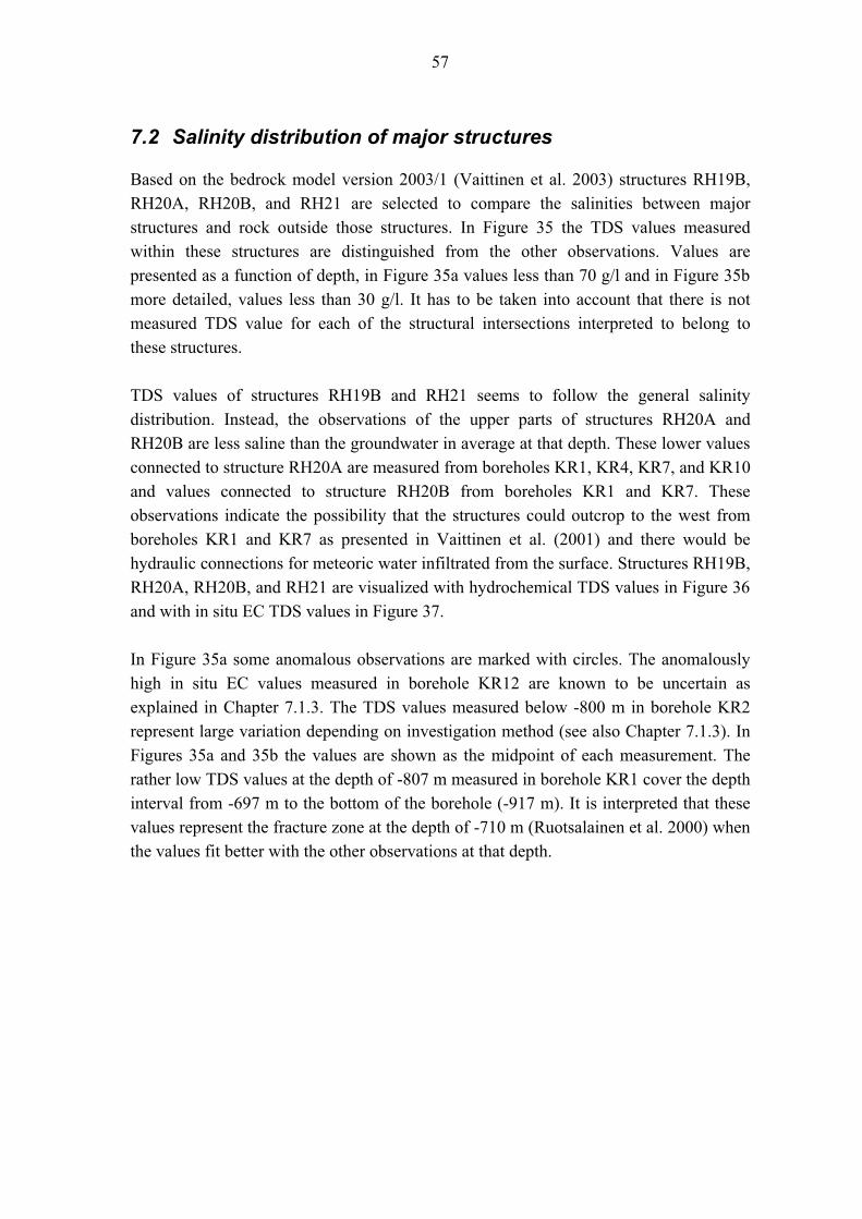
57

7.2 Salinity distribution of major structures

Based on the bedrock model version 2003/1 (Vaittinen et al. 2003) structures RH19B,

RH20A, RH20B, and RH21 are selected to compare the salinities between major

structures and rock outside those structures. In Figure 35 the TDS values measured

within these structures are distinguished from the other observations. Values are

presented as a function of depth, in Figure 35a values less than 70 g/l and in Figure 35b

more detailed, values less than 30 g/l. It has to be taken into account that there is not

measured TDS value for each of the structural intersections interpreted to belong to

these structures.

TDS values of structures RH19B and RH21 seems to follow the general salinity

distribution. Instead, the observations of the upper parts of structures RH20A and

RH20B are less saline than the groundwater in average at that depth. These lower values

connected to structure RH20A are measured from boreholes KR1, KR4, KR7, and KR10

and values connected to structure RH20B from boreholes KR1 and KR7. These

observations indicate the possibility that the structures could outcrop to the west from

boreholes KR1 and KR7 as presented in Vaittinen et al. (2001) and there would be

hydraulic connections for meteoric water infiltrated from the surface. Structures RH19B,

RH20A, RH20B, and RH21 are visualized with hydrochemical TDS values in Figure 36

and with in situ EC TDS values in Figure 37.

In Figure 35a some anomalous observations are marked with circles. The anomalously

high in situ EC values measured in borehole KR12 are known to be uncertain as

explained in Chapter 7.1.3. The TDS values measured below -800 m in borehole KR2

represent large variation depending on investigation method (see also Chapter 7.1.3). In

Figures 35a and 35b the values are shown as the midpoint of each measurement. The

rather low TDS values at the depth of -807 m measured in borehole KR1 cover the depth

interval from -697 m to the bottom of the borehole (-917 m). It is interpreted that these

values represent the fracture zone at the depth of -710 m (Ruotsalainen et al. 2000) when

the values fit better with the other observations at that depth.

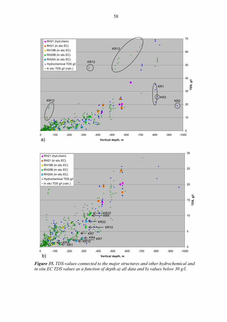
58

0

5

10

15

20

25

30

-1000-900-800-700-600-500-400-300-200-1000

Vertical depth, m

TD

S,

g/l

RH21 (hyd.chem)

RH21 (in situ EC)

RH19B (in situ EC)

RH20B (in situ EC)

RH20A (in situ EC)

Hydrochemical TDS g/l

In situ TDS g/l (calc.)

0

10

20

30

40

50

60

70

-1000-900-800-700-600-500-400-300-200-1000

Vertical depth, m

TD

S,

g/l

RH21 (hyd.chem)

RH21 (in situ EC)

RH19B (in situ EC)

RH20B (in situ EC)

RH20A (in situ EC)

Hydrochemical TDS g/l

In situ TDS g/l (calc.)

KR12

KR12

KR12 KR2KR2

KR1

KR4

KR22

KR10

KR7

KR1 KR10

KR4

KR1

KR22

KR7

a)

b)

0

5

10

15

20

25

30

-1000-900-800-700-600-500-400-300-200-1000

Vertical depth, m

TD

S,

g/l

RH21 (hyd.chem)

RH21 (in situ EC)

RH19B (in situ EC)

RH20B (in situ EC)

RH20A (in situ EC)

Hydrochemical TDS g/l

In situ TDS g/l (calc.)

0

10

20

30

40

50

60

70

-1000-900-800-700-600-500-400-300-200-1000

Vertical depth, m

TD

S,

g/l

RH21 (hyd.chem)

RH21 (in situ EC)

RH19B (in situ EC)

RH20B (in situ EC)

RH20A (in situ EC)

Hydrochemical TDS g/l

In situ TDS g/l (calc.)

KR12

KR12

KR12 KR2KR2

KR1

KR4

KR22

KR10

KR7

KR1 KR10

KR4

KR1

KR22

KR7

a)

b)

Figure 35. TDS-values connected to the major structures and other hydrochemical and

in situ EC TDS values as a function of depth a) all data and b) values below 30 g/l.

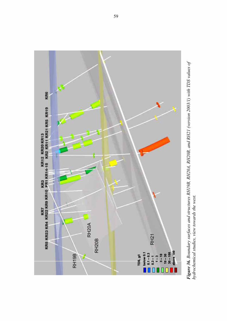
59

TD

S,

g/l

be

low

0.1

0.1

–0

.30

.3–

11

–3

3–

1010

–30

30–

100

abo

ve 1

00

RH

19B

RH

20

A

RH

20

B

RH

21

TD

S,

g/l

be

low

0.1

0.1

–0

.30

.3–

11

–3

3–

1010

–30

30–

100

abo

ve 1

00

TD

S,

g/l

be

low

0.1

0.1

–0

.30

.3–

11

–3

3–

1010

–30

30–

100

abo

ve 1

00

RH

19B

RH

20

A

RH

20

B

RH

21

Fig

ure

36

. B

oundary

surf

ace

s and s

truct

ure

s R

H19B

, R

H20A

, R

H20B

, and R

H21 (

vers

ion 2

003/1

) w

ith T

DS v

alu

es o

f

hyd

roch

emic

al

stu

die

s, v

iew

to

wa

rds

the

wes

t.

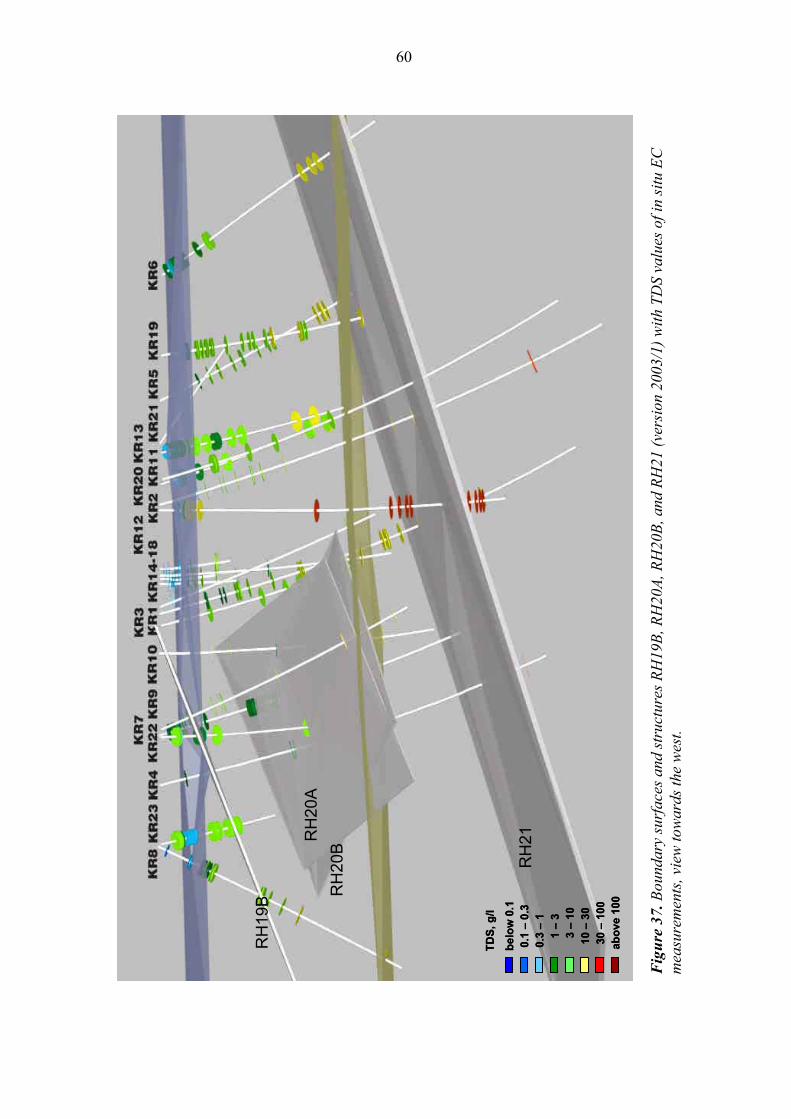
60

RH

19B

RH

20A

RH

20

B

RH

21

TD

S,

g/l

be

low

0.1

0.1

–0

.30

.3–

11

–3

3–

10

10

–3

030

–10

0ab

ove

100

RH

19B

RH

20A

RH

20

B

RH

21

TD

S,

g/l

be

low

0.1

0.1

–0

.30

.3–

11

–3

3–

10

10

–3

030

–10

0ab

ove

100

TD

S,

g/l

be

low

0.1

0.1

–0

.30

.3–

11

–3

3–

10

10

–3

030

–10

0ab

ove

100

Fig

ure

37

. B

oundary

surf

ace

s and s

truct

ure

s R

H19B

, R

H20A

, R

H20B

, and R

H21 (

vers

ion 2

003/1

) w

ith T

DS v

alu

es o

f in

sit

u E

C

mea

sure

men

ts,

view

tow

ard

s th

e w

est.

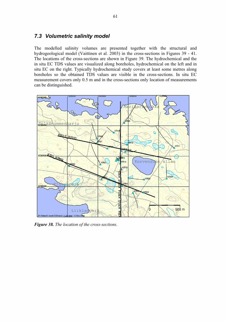
61

7.3 Volumetric salinity model

The modelled salinity volumes are presented together with the structural andhydrogeological model (Vaittinen et al. 2003) in the cross-sections in Figures 39 - 41.The locations of the cross-sections are shown in Figure 39. The hydrochemical and thein situ EC TDS values are visualized along boreholes, hydrochemical on the left and insitu EC on the right. Typically hydrochemical study covers at least some metres alongboreholes so the obtained TDS values are visible in the cross-sections. In situ ECmeasurement covers only 0.5 m and in the cross-sections only location of measurements can be distinguished.

Figure 38. The location of the cross-sections.

62

Fig

ure

39

. T

he

cross

-sec

tion o

f th

e vo

lum

etri

c m

odel

conta

inin

g t

he

sali

nit

y m

odel

, th

e st

ruct

ura

l m

odel

and t

he

hyd

rogeo

logic

al

model

(ve

rsio

n 2

003/1

).

63

Fig

ure

40

. T

he

cross

-sec

tion o

f th

e vo

lum

etri

c m

odel

conta

inin

g t

he

sali

nit

y m

odel

, th

e st

ruct

ura

l m

odel

and t

he

hyd

rogeo

logic

al

model

(ve

rsio

n 2

003/1

).

64

Fig

ure

41

. T

he

cross

-sec

tion o

f th

e vo

lum

etri

c m

odel

conta

inin

g t

he

sali

nit

y m

odel

, th

e st

ruct

ura

l m

odel

and t

he

hyd

rogeo

logic

al

model

(ve

rsio

n 2

003/1

).

65

8 DISCUSSION

This report presents the work conducted to create an updated groundwater TDS salinity

distribution of the Olkiluoto Island. The model has been compiled from hydrochemical

TDS analyses, and from TDS values computed of EC measurements of hydrological

flow logging data. There are plenty of real observations now available. However the

observation data is not continuous in boreholes or over site volume, and is unevenly

distributed.

The model has been presented as two simplified boundary surfaces, and three

subvolumes of increasing salinity according to depth, i.e., TDS<1 g/l, TDS: 1-10 g/l, and

TDS>10 g/l. All observation data support this general trend. The volumes are not of

uniform salinity, but display increase with depth until the next boundary surface is met.

The boundary surfaces described here are in fact diffuse boundaries rather than sharp

surfaces.

The downwards increasing salinity has been reasoned from evolution of the groundwater

species, c.f. (Luukkonen et al. 2003), were the longest residence time fluids with long

period of interaction with host rock have been mixed with more recent water species

during the time. These recent water types are variable of origin, including ancient phases

of Baltic Sea (Litorina Sea among the others), glacial melt waters, the current Baltic Sea

brackish water, and finally the most recent meteoric water infiltration.

There will exist geological reasons for occurrence of the saline groundwaters, e.g., the

hydrothermal processes during ductile deformation or later events; the occurrence of

pyrite and graphite minerals in host rock, etc. Heterogeneities may emerge from recent

interaction and dilution with fresh waters in fracture zones. The distribution has been

presented here as if the bedrock pore water would have same properties with the water

obtained from the fractures with sampling.

The conceptual model is a simplification, which takes smoothed approach compared to

previous more complex shaped model (Heikkinen et al. 1996). The selection for the

form of bounding surfaces will now enhance the planarity of the observations.

Deductions on the coincidence of structure positions and orientations with respect to this

presentation would require more data in future. The deviations of single observations

from the general trend may bring in some indications on the influence of the fracture

structures.

The observations have been emphasized in this work. The boundaries of the classes have

been fit according to maximum or minimum values of the salinity belonging to each

66

class. Purpose has been to enable viewing of the observations in vertical cross sections

and maps, along with bedrock model structures, rock types and borehole data. On the

boundary surfaces, the apparent positions of them according to their fit to the data would

suggest very horizontal orientation. General trend of the dip direction is pointing

towards southerly direction (southwest….southeast).

The data for assessing any influence of the fracture structures or topography is

inadequate. There are no direct indications from the model of such features, except the

single deviating values at RH20B alternative location in KR1 (152 m) and KR06_6R in

KR6 (124 m). Such deviations are scattered within the larger volume of other class,

without forming any clear undulations on the boundary, or established sub-volumes of

other class within the major volume. Neither any deduction alike can be made according

to the data yet.

The geophysical data has been in previous work the basis for modeling. Still in this

phase of the work, it was expected to gain supplement for the exact analysis data and

locations from the geophysical logging along the boreholes and electromagnetic

sounding results between the boreholes and outside the area covered by boreholes.

However, the use of geophysical results seems to require complementary processing of

the data to remove other features influencing on the measurement. These features may

be for logging data tool effects coupled with an influence of saline water in open

borehole (which needs to be corrected for), or drilling water effects, and open borehole

flows. Further to this, it would be required to define the strongly varying porosity and

formation factor in the bedrock, and use these together with bulk resistivity to define the

bedrock pore water salinity. During 3-D visualization and modeling it became evident

that the electrically conductive horizons dominate the EM response, which thus cannot

be directly used without more comprehensive EM modeling. Thus the geophysical data

has been applied in a tentative manner in this report.

Most reliable results can be obtained with both hydrochemical sampling and flow

logging, when the data is representative of the specific depth interval (the fracture zone

where water has been obtained). This condition holds when:

- point like pumping source involved in sampling has not caused intrusion through

fractures from outside of pumping section

- line source pumping in flow logging has not raised saline water upwards in

borehole, nor that water intruded into fractures.

These possibilities have been considered in cases where the data deviated from general

trends. Other limitations of methods have been discussed in Ruotsalainen et al. (2000).

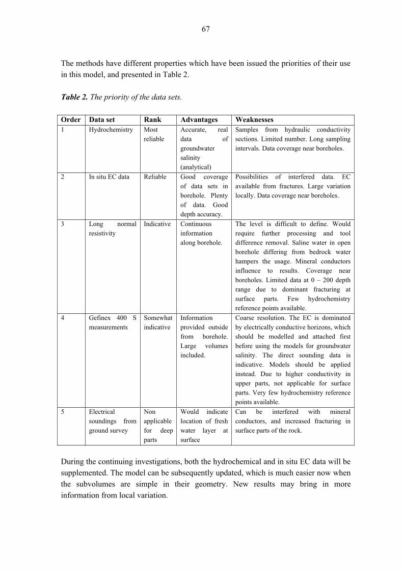
67

The methods have different properties which have been issued the priorities of their use

in this model, and presented in Table 2.

Table 2. The priority of the data sets.

Order Data set Rank Advantages Weaknesses

1 Hydrochemistry Most

reliable

Accurate, real

data of

groundwater

salinity

(analytical)

Samples from hydraulic conductivity

sections. Limited number. Long sampling

intervals. Data coverage near boreholes.

2 In situ EC data Reliable Good coverage

of data sets in

borehole. Plenty

of data. Good

depth accuracy.

Possibilities of interfered data. EC

available from fractures. Large variation

locally. Data coverage near boreholes.

3 Long normal

resistivity

Indicative Continuous

information

along borehole.

The level is difficult to define. Would

require further processing and tool

difference removal. Saline water in open

borehole differing from bedrock water

hampers the usage. Mineral conductors

influence to results. Coverage near

boreholes. Limited data at 0 – 200 depth

range due to dominant fracturing at

surface parts. Few hydrochemistry

reference points available.

4 Gefinex 400 S

measurements

Somewhat

indicative

Information

provided outside

from borehole.

Large volumes

included.

Coarse resolution. The EC is dominated

by electrically conductive horizons, which

should be modelled and attached first

before using the models for groundwater

salinity. The direct sounding data is

indicative. Models should be applied

instead. Due to higher conductivity in

upper parts, not applicable for surface

parts. Very few hydrochemistry reference

points available.

5 Electrical

soundings from

ground survey

Non

applicable

for deep

parts

Would indicate

location of fresh

water layer at

surface

Can be interfered with mineral

conductors, and increased fracturing in

surface parts of the rock.

During the continuing investigations, both the hydrochemical and in situ EC data will be

supplemented. The model can be subsequently updated, which is much easier now when

the subvolumes are simple in their geometry. New results may bring in more

information from local variation.

68

For representativity reasons described above, and also due to lack of data from TDS

transition zones or diffusion margins, it would be valuable to supplement the data set. A

supplement like this would be specifically valuable from deeper parts of the bedrock

volume, and from the sparsely fractured bedrock. To add coverage of the highest

salinities, now mainly observed in deep boreholes KR1, KR2, KR4, KR7, KR11 and

KR12, would require to extent some of new boreholes to deeper level so that the upper

surface of the class >30 g/l would be presented in the model.

The data is available from area covered by deep boreholes. In case the properties of the

layers need to be reviewed further on, new data would be required. This can be provided

firstly by drilling and sampling/logging on a similar way as until now. Applying the

geophysical EM sounding data would help to some extent, while keeping in mind there

are some requirements for the usage.

Applying the geophysical information from boreholes, would require some further

processing of long normal logging data. Other opportunity is to design a new array or a

combination or several arrays to be applied in boreholes or in crosshole manner to obtain

formation factor and porosity together with salinity, which would better describe the

electrical conductivity of the groundwater residing in host rock. These would be also

applicable for monitoring of any changes in the salinity distribution.

Applying the already existing Gefinex 400S data, all the sounding stations would require

firstly modeling to a detailed, optimized layer model with borehole tie data, and then

usage of the layer thicknesses and EC data for TDS modeling.

The modeling would be essential for monitoring effort, e.g. for selection of the possible

locations for monitoring (best locations). Modeling would be a prejudice for obtaining

salinity estimate outside of area covered by boreholes. Monitoring can apply this model,

follow-up of changes in hydrochemical data and in situ EC data behind this model, and

when properly designed and modeled beforehand, also geophysical borehole data and

electromagnetic sounding models.

Supplementary coverage of data will be gathered during continuing investigations.

These are obtained from boreholes in the central area and surrounding it, as well as from

tunnels when these are constructed. The model data has now been organized and

described so that any further supplement is feasible.

The model presented in this work is descriptive visualization of bedrock groundwater

salinity distribution, and the data density involved. The data and the model can be used

as basis for dynamic flow modeling and simulations of change in salinity to be used in

testing and verifications of monitoring.

69

9 REFERENCES

Ahokas, T. 2003. Electromagnetic frequency soundings (Gefinex 400S) in Olkiluoto2002. Eurajoki, Posiva. Posiva Working report 2003-24, 89 p.

Aittoniemi, K., Rajala, J. and Sarvas, J. 1987. Interactive Inversion Algorithm andApparent Resistivity Versus Depth (ARD) plot in Multifrequency Depth Soundings.Acta Polytechnica Scandinavica, Applied Physics Series No. 157, Helsinki 1987, 34 pp.

Blomqvist, R. (1999). Hydrogeochemistry of deep groundwaters in the central part ofthe Fennoscandian Shield. Espoo, Finland: Geological Survey of Finland, Nuclear Waste Disposal Research. 41 p. Report YST-101.

Blomqvist, R., Nissinen, P., Frape, S. (1992) Dating of fracture minerals from Olkiluoto in Eurajoki (in Finnish with an English abstract). Helsinki, Finland: Teollisuuden Voima Oy. 188 p. Site Investigations, Work Report 92-27.

Blyth, A., Frape, S., Blomqvist, R., Nissinen, P. & McNutt, R. (1998) An isotopic andfluid inclusion study of fracture calcite from borehole OL-KR1 at the Olkiluoto site,Finland. Helsinki, Finland: Posiva Oy. 56 p. Report POSIVA-98-04.

Brace, W.F., Orange, A. & Madden, T. 1965. The effect of pressure on the electricalresistivity of water-saturated crystalline rocks. J. Geophys. Res. 70, 22, pp. 5669 – 5678.

Dakhnov, V. N. 1962. Geophysical well logging. Originally published in Moscow 1959. Translated by Keller, V. 1962. In Quarterly of the Colorado School of Mines, Vol. 57,no. 2.

Davis, S.N. (1964) The chemistry of saline waters. In: Krieger, R.A. - Discussion.Groundwater, vol 2(1), 51.

Frape, S.K. & Fritz, P. (1987). Geochemical trends from groundwaters from theCanadian Shield. In: Fritz, P. & Frape, S.K. (eds.) Saline waters and gases in crystalline rocks. Geol. Assoc. Canada Spec. Paper 33, p. 19-38.

Gascoyne, M., Ross, J.D., Watson, R.L. (1996). Highly saline pore fluids in the rockmatrix of a granitic batholith on the Canadian Shield. Paper presented at the 30th

International Geological Congress, Beijing, China, August 1996.

Hallenburg, J.K. 1984. Geophysical logging for mineral and engineering applications.Tulsa, Penwell, 254 p.

Heikkinen, E., Ahokas, T. & Saksa, P. 2004a. Interpretation of Olkiluoto electromagnetic Gefinex 400S soundings and pole-pole electrical soundings. Eurajoki,Posiva Ltd. Posiva Working report 2004-16, 180 p.

Heikkinen, E., Hellä, P., Saksa, P., Palmén, J. and Vaittinen, T. 2004b. Unification of electrical resistivity logging data. Eurajoki, Posiva Ltd. Posiva Working report 2004-xx.129 p. (in print).

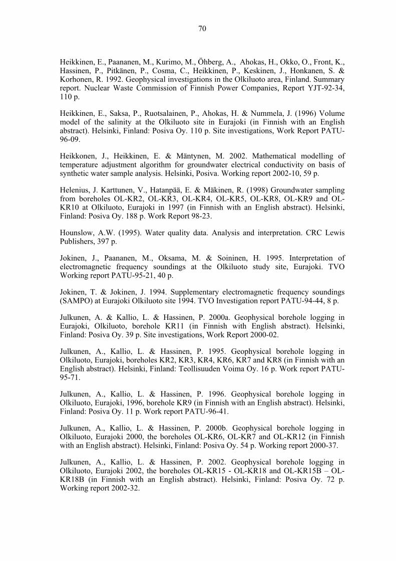
70

Heikkinen, E., Paananen, M., Kurimo, M., Öhberg, A., Ahokas, H., Okko, O., Front, K., Hassinen, P., Pitkänen, P., Cosma, C., Heikkinen, P., Keskinen, J., Honkanen, S. &Korhonen, R. 1992. Geophysical investigations in the Olkiluoto area, Finland. Summary report. Nuclear Waste Commission of Finnish Power Companies, Report YJT-92-34,110 p.

Heikkinen, E., Saksa, P., Ruotsalainen, P., Ahokas, H. & Nummela, J. (1996) Volumemodel of the salinity at the Olkiluoto site in Eurajoki (in Finnish with an Englishabstract). Helsinki, Finland: Posiva Oy. 110 p. Site investigations, Work Report PATU-96-09.

Heikkonen, J., Heikkinen, E. & Mäntynen, M. 2002. Mathematical modelling oftemperature adjustment algorithm for groundwater electrical conductivity on basis ofsynthetic water sample analysis. Helsinki, Posiva. Working report 2002-10, 59 p.

Helenius, J. Karttunen, V., Hatanpää, E. & Mäkinen, R. (1998) Groundwater samplingfrom boreholes OL-KR2, OL-KR3, OL-KR4, OL-KR5, OL-KR8, OL-KR9 and OL-KR10 at Olkiluoto, Eurajoki in 1997 (in Finnish with an English abstract). Helsinki,Finland: Posiva Oy. 188 p. Work Report 98-23.

Hounslow, A.W. (1995). Water quality data. Analysis and interpretation. CRC LewisPublishers, 397 p.

Jokinen, J., Paananen, M., Oksama, M. & Soininen, H. 1995. Interpretation ofelectromagnetic frequency soundings at the Olkiluoto study site, Eurajoki. TVOWorking report PATU-95-21, 40 p.

Jokinen, T. & Jokinen, J. 1994. Supplementary electromagnetic frequency soundings(SAMPO) at Eurajoki Olkiluoto site 1994. TVO Investigation report PATU-94-44, 8 p.

Julkunen, A. & Kallio, L. & Hassinen, P. 2000a. Geophysical borehole logging inEurajoki, Olkiluoto, borehole KR11 (in Finnish with English abstract). Helsinki,Finland: Posiva Oy. 39 p. Site investigations, Work Report 2000-02.

Julkunen, A., Kallio, L. & Hassinen, P. 1995. Geophysical borehole logging inOlkiluoto, Eurajoki, boreholes KR2, KR3, KR4, KR6, KR7 and KR8 (in Finnish with an English abstract). Helsinki, Finland: Teollisuuden Voima Oy. 16 p. Work report PATU-95-71.

Julkunen, A., Kallio, L. & Hassinen, P. 1996. Geophysical borehole logging inOlkiluoto, Eurajoki, 1996, borehole KR9 (in Finnish with an English abstract). Helsinki,Finland: Posiva Oy. 11 p. Work report PATU-96-41.

Julkunen, A., Kallio, L. & Hassinen, P. 2000b. Geophysical borehole logging inOlkiluoto, Eurajoki 2000, the boreholes OL-KR6, OL-KR7 and OL-KR12 (in Finnishwith an English abstract). Helsinki, Finland: Posiva Oy. 54 p. Working report 2000-37.

Julkunen, A., Kallio, L. & Hassinen, P. 2002. Geophysical borehole logging inOlkiluoto, Eurajoki 2002, the boreholes OL-KR15 - OL-KR18 and OL-KR15B – OL-KR18B (in Finnish with an English abstract). Helsinki, Finland: Posiva Oy. 72 p.Working report 2002-32.

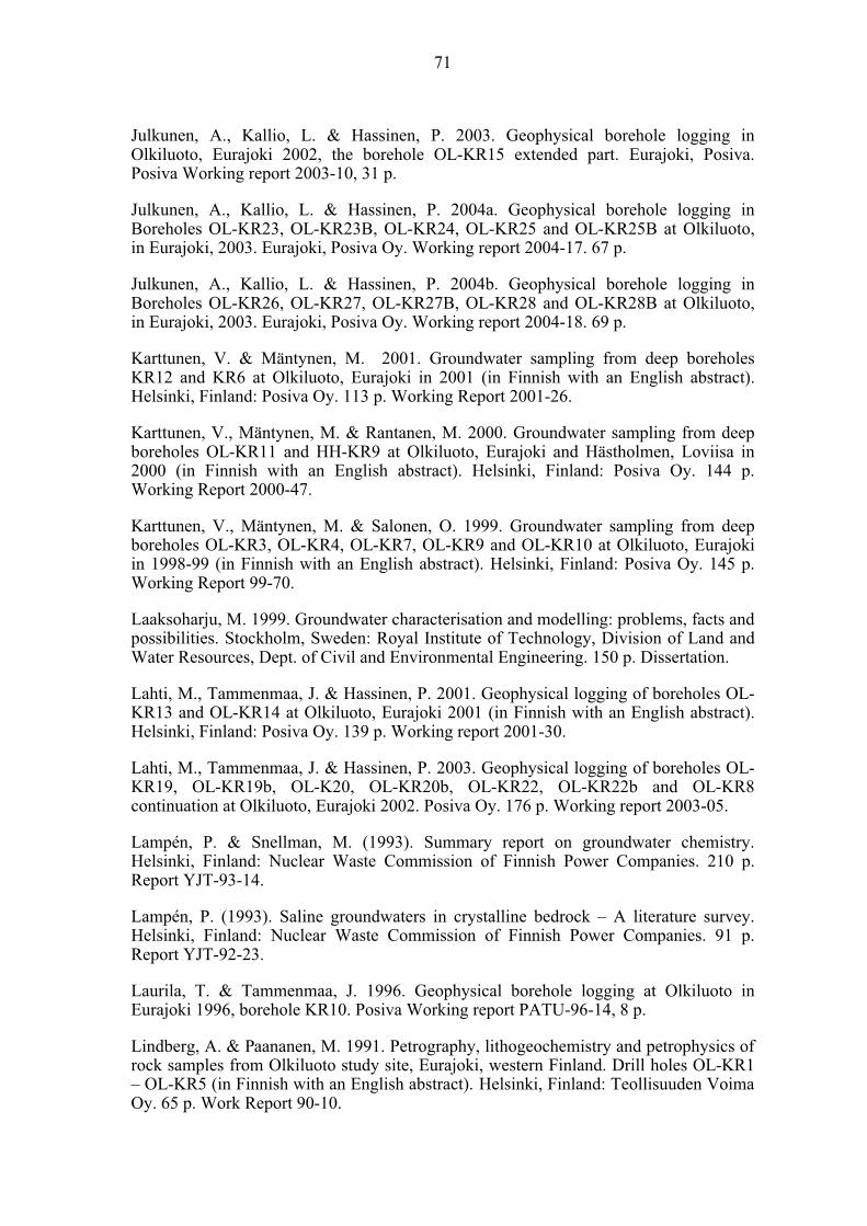
71

Julkunen, A., Kallio, L. & Hassinen, P. 2003. Geophysical borehole logging inOlkiluoto, Eurajoki 2002, the borehole OL-KR15 extended part. Eurajoki, Posiva.Posiva Working report 2003-10, 31 p.

Julkunen, A., Kallio, L. & Hassinen, P. 2004a. Geophysical borehole logging inBoreholes OL-KR23, OL-KR23B, OL-KR24, OL-KR25 and OL-KR25B at Olkiluoto,in Eurajoki, 2003. Eurajoki, Posiva Oy. Working report 2004-17. 67 p.

Julkunen, A., Kallio, L. & Hassinen, P. 2004b. Geophysical borehole logging inBoreholes OL-KR26, OL-KR27, OL-KR27B, OL-KR28 and OL-KR28B at Olkiluoto,in Eurajoki, 2003. Eurajoki, Posiva Oy. Working report 2004-18. 69 p.

Karttunen, V. & Mäntynen, M. 2001. Groundwater sampling from deep boreholesKR12 and KR6 at Olkiluoto, Eurajoki in 2001 (in Finnish with an English abstract).Helsinki, Finland: Posiva Oy. 113 p. Working Report 2001-26.

Karttunen, V., Mäntynen, M. & Rantanen, M. 2000. Groundwater sampling from deepboreholes OL-KR11 and HH-KR9 at Olkiluoto, Eurajoki and Hästholmen, Loviisa in2000 (in Finnish with an English abstract). Helsinki, Finland: Posiva Oy. 144 p.Working Report 2000-47.

Karttunen, V., Mäntynen, M. & Salonen, O. 1999. Groundwater sampling from deepboreholes OL-KR3, OL-KR4, OL-KR7, OL-KR9 and OL-KR10 at Olkiluoto, Eurajokiin 1998-99 (in Finnish with an English abstract). Helsinki, Finland: Posiva Oy. 145 p.Working Report 99-70.

Laaksoharju, M. 1999. Groundwater characterisation and modelling: problems, facts and possibilities. Stockholm, Sweden: Royal Institute of Technology, Division of Land andWater Resources, Dept. of Civil and Environmental Engineering. 150 p. Dissertation.

Lahti, M., Tammenmaa, J. & Hassinen, P. 2001. Geophysical logging of boreholes OL-KR13 and OL-KR14 at Olkiluoto, Eurajoki 2001 (in Finnish with an English abstract).Helsinki, Finland: Posiva Oy. 139 p. Working report 2001-30.

Lahti, M., Tammenmaa, J. & Hassinen, P. 2003. Geophysical logging of boreholes OL-KR19, OL-KR19b, OL-K20, OL-KR20b, OL-KR22, OL-KR22b and OL-KR8continuation at Olkiluoto, Eurajoki 2002. Posiva Oy. 176 p. Working report 2003-05.

Lampén, P. & Snellman, M. (1993). Summary report on groundwater chemistry.Helsinki, Finland: Nuclear Waste Commission of Finnish Power Companies. 210 p.Report YJT-93-14.

Lampén, P. (1993). Saline groundwaters in crystalline bedrock – A literature survey.Helsinki, Finland: Nuclear Waste Commission of Finnish Power Companies. 91 p.Report YJT-92-23.

Laurila, T. & Tammenmaa, J. 1996. Geophysical borehole logging at Olkiluoto inEurajoki 1996, borehole KR10. Posiva Working report PATU-96-14, 8 p.

Lindberg, A. & Paananen, M. 1991. Petrography, lithogeochemistry and petrophysics of rock samples from Olkiluoto study site, Eurajoki, western Finland. Drill holes OL-KR1– OL-KR5 (in Finnish with an English abstract). Helsinki, Finland: Teollisuuden Voima Oy. 65 p. Work Report 90-10.

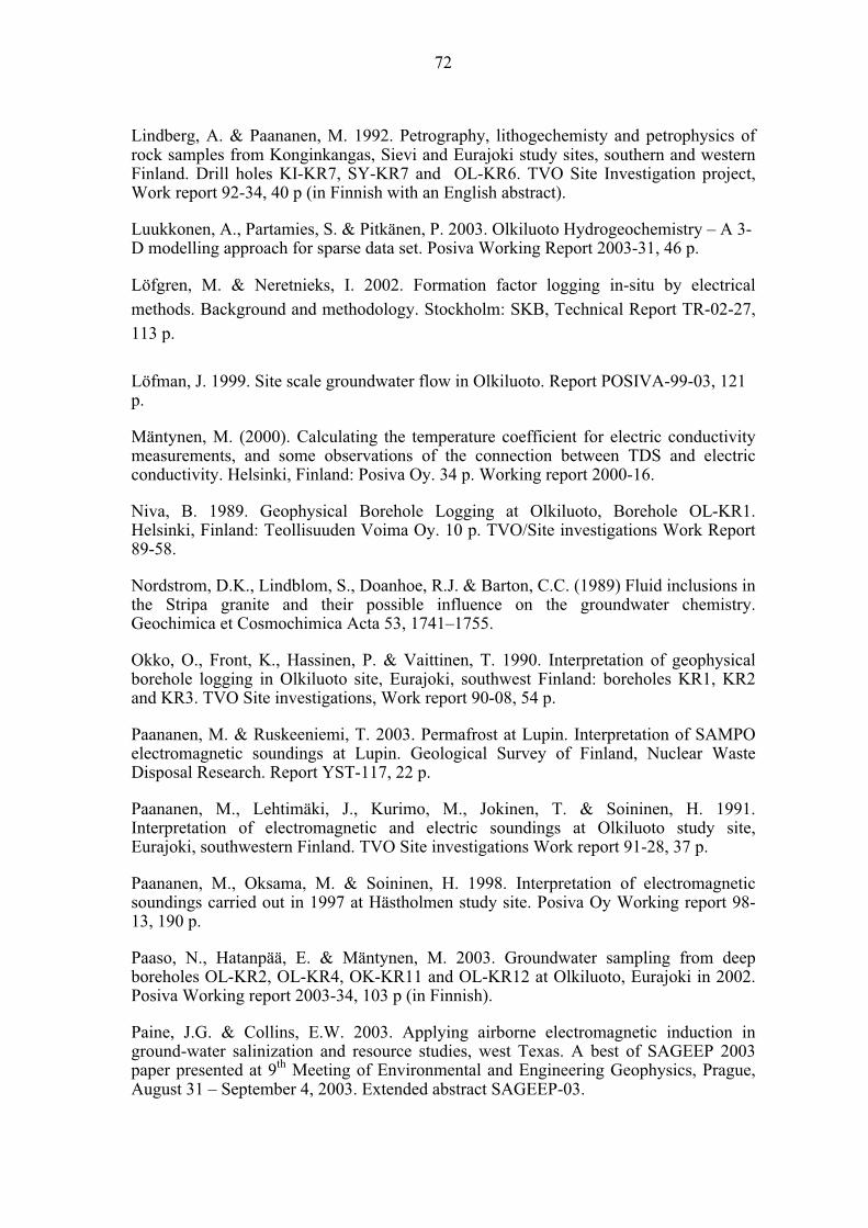
72

Lindberg, A. & Paananen, M. 1992. Petrography, lithogechemisty and petrophysics ofrock samples from Konginkangas, Sievi and Eurajoki study sites, southern and westernFinland. Drill holes KI-KR7, SY-KR7 and OL-KR6. TVO Site Investigation project,Work report 92-34, 40 p (in Finnish with an English abstract).

Luukkonen, A., Partamies, S. & Pitkänen, P. 2003. Olkiluoto Hydrogeochemistry – A 3-D modelling approach for sparse data set. Posiva Working Report 2003-31, 46 p.

Löfgren, M. & Neretnieks, I. 2002. Formation factor logging in-situ by electrical

methods. Background and methodology. Stockholm: SKB, Technical Report TR-02-27,

113 p.

Löfman, J. 1999. Site scale groundwater flow in Olkiluoto. Report POSIVA-99-03, 121 p.

Mäntynen, M. (2000). Calculating the temperature coefficient for electric conductivitymeasurements, and some observations of the connection between TDS and electricconductivity. Helsinki, Finland: Posiva Oy. 34 p. Working report 2000-16.

Niva, B. 1989. Geophysical Borehole Logging at Olkiluoto, Borehole OL-KR1.Helsinki, Finland: Teollisuuden Voima Oy. 10 p. TVO/Site investigations Work Report89-58.

Nordstrom, D.K., Lindblom, S., Doanhoe, R.J. & Barton, C.C. (1989) Fluid inclusions in the Stripa granite and their possible influence on the groundwater chemistry.Geochimica et Cosmochimica Acta 53, 1741–1755.

Okko, O., Front, K., Hassinen, P. & Vaittinen, T. 1990. Interpretation of geophysicalborehole logging in Olkiluoto site, Eurajoki, southwest Finland: boreholes KR1, KR2and KR3. TVO Site investigations, Work report 90-08, 54 p.

Paananen, M. & Ruskeeniemi, T. 2003. Permafrost at Lupin. Interpretation of SAMPOelectromagnetic soundings at Lupin. Geological Survey of Finland, Nuclear WasteDisposal Research. Report YST-117, 22 p.

Paananen, M., Lehtimäki, J., Kurimo, M., Jokinen, T. & Soininen, H. 1991.Interpretation of electromagnetic and electric soundings at Olkiluoto study site,Eurajoki, southwestern Finland. TVO Site investigations Work report 91-28, 37 p.

Paananen, M., Oksama, M. & Soininen, H. 1998. Interpretation of electromagneticsoundings carried out in 1997 at Hästholmen study site. Posiva Oy Working report 98-13, 190 p.

Paaso, N., Hatanpää, E. & Mäntynen, M. 2003. Groundwater sampling from deepboreholes OL-KR2, OL-KR4, OK-KR11 and OL-KR12 at Olkiluoto, Eurajoki in 2002.Posiva Working report 2003-34, 103 p (in Finnish).

Paine, J.G. & Collins, E.W. 2003. Applying airborne electromagnetic induction inground-water salinization and resource studies, west Texas. A best of SAGEEP 2003paper presented at 9th Meeting of Environmental and Engineering Geophysics, Prague,August 31 – September 4, 2003. Extended abstract SAGEEP-03.

73

Palmén J. & Hellä P. 2003. Summary of the water sampling and analysis results at theOlkiluoto site, Eurajoki, SW Finland. Eurajoki: Posiva Oy. 82 p. Working Report-03-19.

Parkhomenko, E. I. (1967). Electrical properties of rocks. Moscow, Institute of Physicsof the Earth, Academy of the Sciences of the USSR, 277 p.

Pitkänen, P., Luukkonen, A., Ruotsalainen, P, Leino-Forsman, H. & Vuorinen, U.(1999). Geochemical modelling of groundwater evolution and residence time at theOlkiluoto site. Helsinki, Finland: Posiva Oy. 184 p. Report POSIVA-98-10.

Pitkänen, P., Snellman, M. & Leino-Forsman, H. (1994). Geochemical modelling of the groundwater at the Olkiluoto site. Helsinki, Finland: Nuclear Waste Commission ofFinnish Power Companies. 79 p. Report YJT-94-10.

Pitkänen, P., Snellman, M. & Vuorinen, U. (1996). On the origin and chemical evolution of groundwater at the Olkiluoto site. Helsinki, Finland: Posiva Oy. 44 p. ReportPOSIVA-96-04.

Pitkänen, P., Snellman, M., & Leino-Forsman, H. (1993). Vertical distribution ofgroundwater chemistry at Romuvaara, Kivetty and Olkiluoto (in Finnish with an English abstract). Helsinki, Finland: Teollisuuden Voima Oy. 49 p. Work report TURVA-93-03.

Pitkänen, P., Snellman, M., Leino-Forsman, H & Front, K. (1992). Groundwaterchemistry and water-rock interaction at Olkiluoto. Helsinki, Finland: Nuclear WasteCommission of Finnish Power Companies. 92 p. Report YJT-92-02.

Poikonen, A. 1983a. Application of electrical and thermal borehole logging to structural and hydrogeological investigations of crystalline bedrock. VTT Technical ResearchCentre, Research Reports 212, 80 p.

Poikonen. A. 1983b. Suitability of certain borehole geophysical methods for structuraland hydrogeological studies of Finnish bedrock in connection with disposal of nuclearwaste. Nuclear Waste Commission of Finnish Power Companies, Report YJT-83-06, 59p.

Pöllänen, J. & Rouhiainen, P. 2000a. Difference flow measurements at the Olkiluoto site in Eurajoki, borehole KR11. Helsinki, Posiva Oy. Working report 2000-38. 68 p.

Pöllänen, J. & Rouhiainen, P. 2000b. Difference flow and electric conductivitymeasurements at the Olkiluoto site in Eurajoki, boreholes KR6, KR7 and KR12.Helsinki, Posiva Oy. Working report 2000-51. 150 p.

Pöllänen, J. & Rouhiainen, P. 2001a. Difference flow and electric conductivitymeasurements at the Olkiluoto site in Eurajoki, boreholes KR13 – KR14. Helsinki,Posiva Oy. Working report 2001-42. 100 p.

Pöllänen, J. & Rouhiainen, P. 2001b. Flow and electric conductivity measurementsduring long term pumping of borehole KR6 at the Olkiluoto. Helsinki, Posiva Oy.Working report 2001-43.

Pöllänen, J. & Rouhiainen, P. 2002a. Difference flow and electric conductivitymeasurements at the Olkiluoto site in Eurajoki, boreholes KR15 - KR18 and KR15B -KR18B. Posiva Oy. Working report 2002-29. 134 p.

74

Pöllänen, J. & Rouhiainen, P. 2002b. Difference flow and electric conductivitymeasurements at the Olkiluoto site in Eurajoki, extended part of borehole KR15. Posiva Oy. Working report 2002-43. 57 p.

Rantanen, M., Paaso, N. & Mäntynen, M. 2002. Groundwater sampling from deepboreholes KR9 and KR11 and surface water sampling from Korvensuo reservoir atOlkiluoto, Eurajoki in 2001 (in Finnish with an English abstract). Helsinki, Finland:Posiva Oy. 81 p. Working Report 2002-19.

Rouhiainen, P. Geophysical borehole methods in fracture analysis of crystalline bedrock of the Loviisa site. Nuclear Waste Commission of Finnish Power Companies, ReportYJT-89-01, 113 p.

Rouhiainen, P., Doe, T. & Distinguin, M. 2004. Applications of flow logging atradioactive waste research laboratories in France and Sweden. 66th EAGE Conferenceand Exhibition, Paris 7-10 June 2004, Extended Abstracts H006.

Rouhiainen, P. 1999. Electrical conductivity and detailed flow logging at the Olkiluotosite, in Eurajoki, boreholes KR1–KR11. Volume 1: Report and Appendices 1 – 5.Volume 2: Appendices 5 – 13. Helsinki, Finland: Posiva Oy. 387 p. Site Investigations,Working Report 99-72.

Rouhiainen, P. 1994. Difference flow measurements with TVO-flowmeter, description of the method and equipment (in Finnish with an English abstract). Helsinki, Finland: Teollisuuden Voima Oy. Work report PATU-94-24.

Rouhiainen, P., Lampén, P., Snellman, M. & Helenius, J. (1992). Water samplingequipment. Technical description and operating instructions. Rev. III (in Finnish withEnglish abstract). Helsinki, Finland: Teollisuuden Voima Oy. 101 p. Site investigations, Work Report PATU-92-71.

Ruotsalainen, P. & Snellman, M. (1996). Hydrogeochemical baseline characterisation at Romuvaara, Kivetty and Olkiluoto. Helsinki, Finland: Posiva Oy. 109 p. Siteinvestigations, Work Report PATU-96-91e.

Ruotsalainen, P. (ed.), Salonen, O. (ed.), Hatanpää, E., Helenius, J., Karttunen, V.,Keinonen, M., Laakso, T., Rantanen, M. & Sellge, R. (1998). Field manual for watersampling of Posiva. Updated version. Helsinki, Finland: Posiva Oy. 130 p. Siteinvestigations, work report 98-54, rev. 2.

Ruotsalainen, P., Ahokas, H., Heikkinen, E., Lindh, J., Nummela, J. 2000. Groundwatersalinity at the Olkiluoto site. Helsinki, Posiva. Posiva Working Report 2000-26, 103 p.

Savoye, S., Aranyossy, J-F., Beaucaire, C., Cathelineau, M., Louvat, D. & Michelot, J-L. (1998). Fluid inclusions in granites and their relationships with present-daygroundwater chemistry. Eur. J. Mineral., 10, pp. 1215-1226.

SFS (1994). Water quality, determination of electrical conductivity, SFS-EN 27888.

Sipola, V-P. 2002. A new data processing- and interpretation program for the Sampoelectromagnetic multifrequency sounding system. Masters thesis, Helsinki University of Technology, Department of Materials Science and Rock Engineering, 2002. In Finnish.

75

Smith, B.D. and Ward S. H.,1974. On the computation of polarization ellipseparameters. Geophysics, vol. 39, no. 6, December 1974, p. 867-869.

Snellman, M. (1991). Summary report on groundwater chemistry at Olkiluoto, Eurajoki.Helsinki, Finland: Teollisuuden Voima Oy. 61 p. Site investigations, Work Report 91-34.

Snellman, M. 1995. TVO:n käytetyn polttoaineen alustavan sijoituspaikkatutkimus-vaiheen pohjavesikemian tiedosto - TVODATAC (in Finnish with an English abstract).Helsinki, Finland: Teollisuuden Voima Oy. 8 p. Work Report PATU-95-18.

Soininen, H. 1986. Wideband EM research. Geological Survey of Finland, annual report of the department of geophysics, 1986, pages 50-55. In Finnish (Laajakaista EMtutkimus. Geologian tutkimuskeskus, geofysiikan osaston toimintakertomus, 1986, s. 50-55).

Stratton, J. A. 1941. Electromagnetic theory. McGraw-Hill.

Suomen Malmi Oy 1989c. Geophysical Borehole Logging in Olkiluoto, Eurajoki,Boreholes KR2 and KR3 (in Finnish with an English abstract). Helsinki, Finland:Teollisuuden Voima Oy. 9 p. TVO/Site investigations Work Report 89-88.

Suomen Malmi Oy 1990b. Geophysical Borehole Logging at Olkiluoto InvestigationSite, Boreholes KR4 and KR5 (in Finnish with an English abstract). Helsinki, Finland:Teollisuuden Voima Oy. 9 p. TVO/Site investigations Work Report 90-44.

Tuominen, M. (1994). Sampling and analysis of the environmental reference watersamples in Olkiluoto, 1994 (in Finnish with English abstract). Helsinki, Finland:Teollisuuden Voima Oy. 8 p. Site investigations, Work Report PATU-94-35.

Vaittinen, T. 1988. Kallioreikätutkimusten tulosten käsittely- ja tulkintaohjelma LOG.

Espoo: VTT Technical Research Centre, Research Notes 922, 19 p. (Bedrock borehole

processing and interpretation software LOG, in Finnish).

Vaittinen, T., Ahokas, H., Heikkinen, E., Hellä, P., Nummela, J., Saksa, P., Tammisto,E., Paulamäki, S., Paananen, M., Front, K. & Kärki, A. 2003. Bedrock model of theOlkiluoto site, version 2003/1. Eurajoki, Finland: Posiva Oy. 266 p. Working Report2003-43.

Öhberg, A. & Rouhiainen, P. 2000. Posiva groundwater flow measuring techniques. Helsinki, Finland, Posiva Oy. POSIVA 2000-12.

Öhberg, A. (1991). Site investigation equipment developed by Teollisuuden Voima Oy.Helsinki, Finland: Nuclear Waste Commission of Finnish Power Companies. 46 p.Report YJT-91-06.

76

77

Appendices

1. Difference Flow meter data source reports

2. Geophysical long normal resistivity logging data reports

3. Geophysical long normal and borehole fluid conductivity results with in situ EC values, from boreholes KR1, KR2, KR4, KR7, KR9, KR11, KR12 and KR19.

4. Geophysical long normal EC values visualized along with model boundaries

5. Geophysical GEFINEX 400S EC values visualized along with model boundaries

78

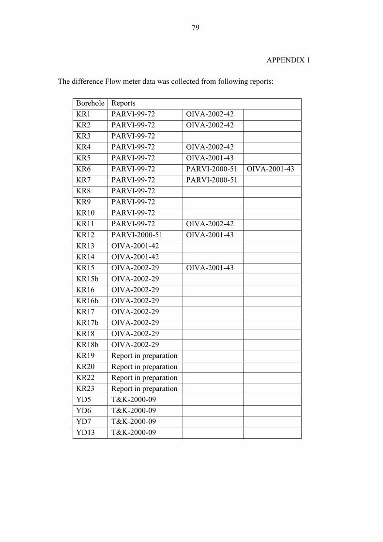
79

APPENDIX 1

The difference Flow meter data was collected from following reports:

Borehole Reports

KR1 PARVI-99-72 OIVA-2002-42

KR2 PARVI-99-72 OIVA-2002-42

KR3 PARVI-99-72

KR4 PARVI-99-72 OIVA-2002-42

KR5 PARVI-99-72 OIVA-2001-43

KR6 PARVI-99-72 PARVI-2000-51 OIVA-2001-43

KR7 PARVI-99-72 PARVI-2000-51

KR8 PARVI-99-72

KR9 PARVI-99-72

KR10 PARVI-99-72

KR11 PARVI-99-72 OIVA-2002-42

KR12 PARVI-2000-51 OIVA-2001-43

KR13 OIVA-2001-42

KR14 OIVA-2001-42

KR15 OIVA-2002-29 OIVA-2001-43

KR15b OIVA-2002-29

KR16 OIVA-2002-29

KR16b OIVA-2002-29

KR17 OIVA-2002-29

KR17b OIVA-2002-29

KR18 OIVA-2002-29

KR18b OIVA-2002-29

KR19 Report in preparation

KR20 Report in preparation

KR22 Report in preparation

KR23 Report in preparation

YD5 T&K-2000-09

YD6 T&K-2000-09

YD7 T&K-2000-09

YD13 T&K-2000-09

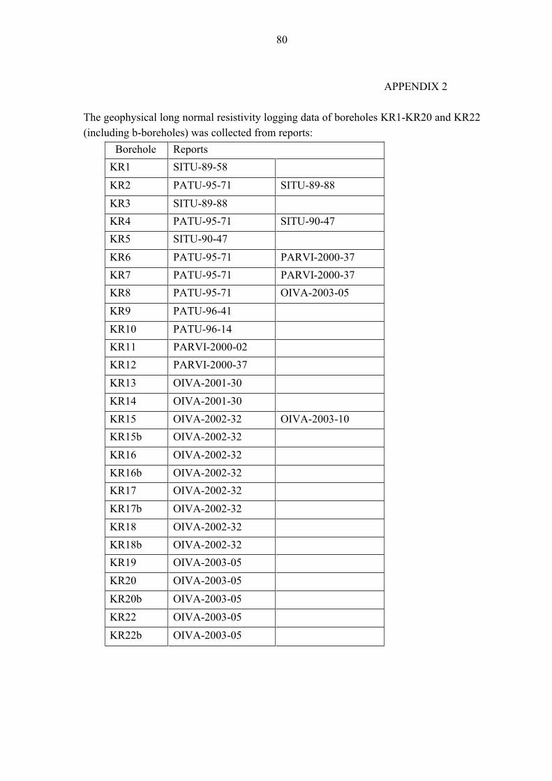
80

APPENDIX 2

The geophysical long normal resistivity logging data of boreholes KR1-KR20 and KR22

(including b-boreholes) was collected from reports:

Borehole Reports

KR1 SITU-89-58

KR2 PATU-95-71 SITU-89-88

KR3 SITU-89-88

KR4 PATU-95-71 SITU-90-47

KR5 SITU-90-47

KR6 PATU-95-71 PARVI-2000-37

KR7 PATU-95-71 PARVI-2000-37

KR8 PATU-95-71 OIVA-2003-05

KR9 PATU-96-41

KR10 PATU-96-14

KR11 PARVI-2000-02

KR12 PARVI-2000-37

KR13 OIVA-2001-30

KR14 OIVA-2001-30

KR15 OIVA-2002-32 OIVA-2003-10

KR15b OIVA-2002-32

KR16 OIVA-2002-32

KR16b OIVA-2002-32

KR17 OIVA-2002-32

KR17b OIVA-2002-32

KR18 OIVA-2002-32

KR18b OIVA-2002-32

KR19 OIVA-2003-05

KR20 OIVA-2003-05

KR20b OIVA-2003-05

KR22 OIVA-2003-05

KR22b OIVA-2003-05

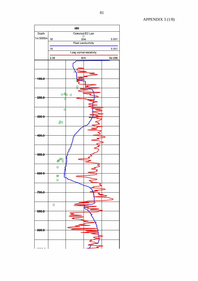
81

APPENDIX 3 (1/8)

# % '

) * + , . + , 0 , 2

#

. 4 . * , , 0 , 2

# 7 7 8 7% '

9 ; <

= > > ? >

@ > > ? >

B > > ? >

C > > ? >

D > > ? >

E > > ? >

F > > ? >

G > > ? >

H > > ? >

= > > > >

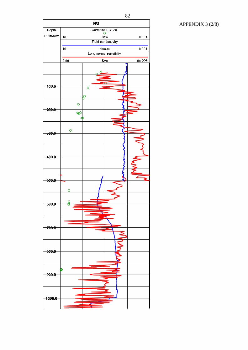
82

APPENDIX 3 (2/8)

# % '

) * + , . + , 0 , 2

# 4

. 7 . * , , 0 , 2

# : : 4 :% '

; = >

? @ @ A @

B @ @ A @

D @ @ A @

E @ @ A @

F @ @ A @

G @ @ A @

H @ @ A @

I @ @ A @

J @ @ A @

? @ @ @ A @

83

APPENDIX 3 (3/8)

# % '

) * + , . + , 0 , 2

# 4

. 7 . * , , 0 , 2

# : : 4 :% '

; = >

? @ @ A @

B @ @ A @

D @ @ A @

E @ @ A @

F @ @ A @

G @ @ A @

H @ @ A @

I @ @ A @

J @ @ @

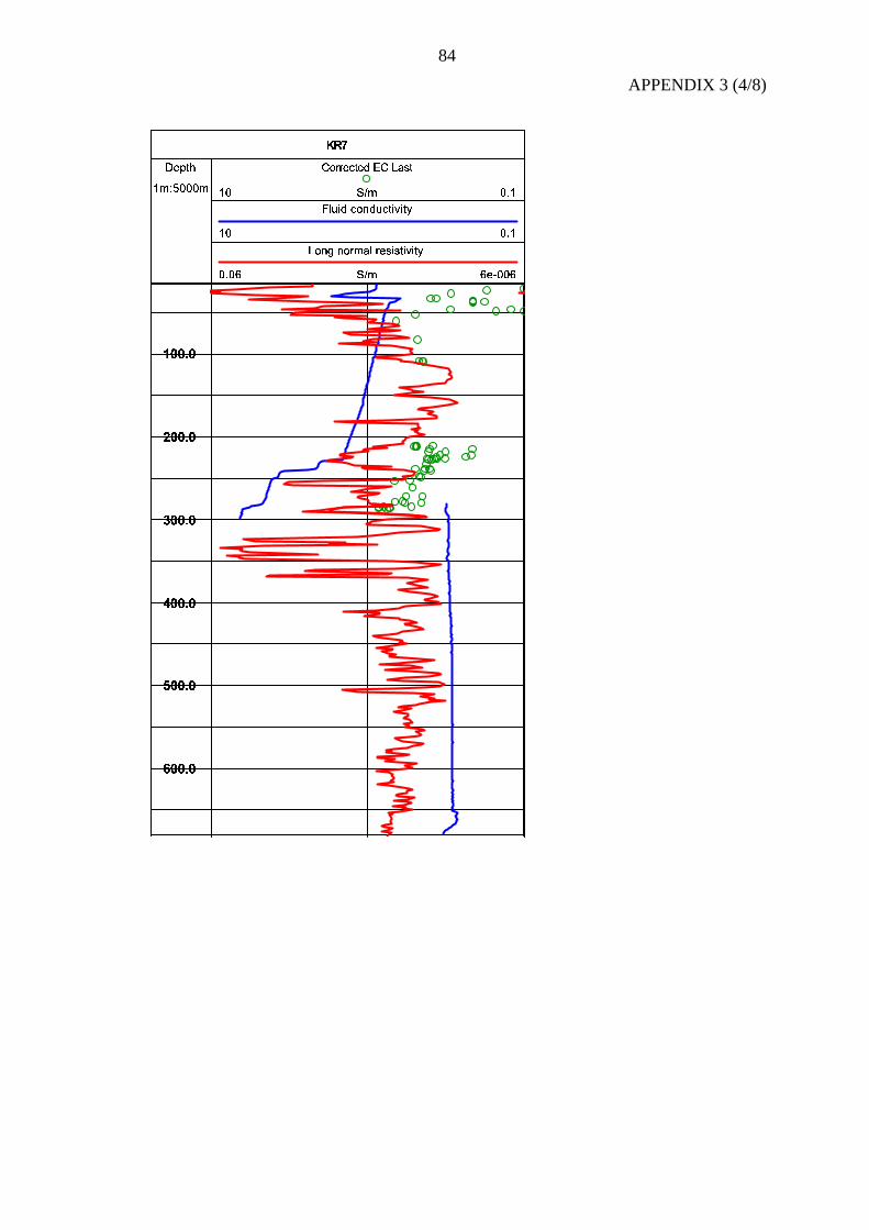
84

APPENDIX 3 (4/8)

" $ &

( ) * + - * + / + 1

"

- 3 - ) + + / + 1

" 6 6 7 6$ &

8 : <

= > > ? >

@ > > ? >

B > > ? >

C > > ? >

D > > ? >

E > > ? >

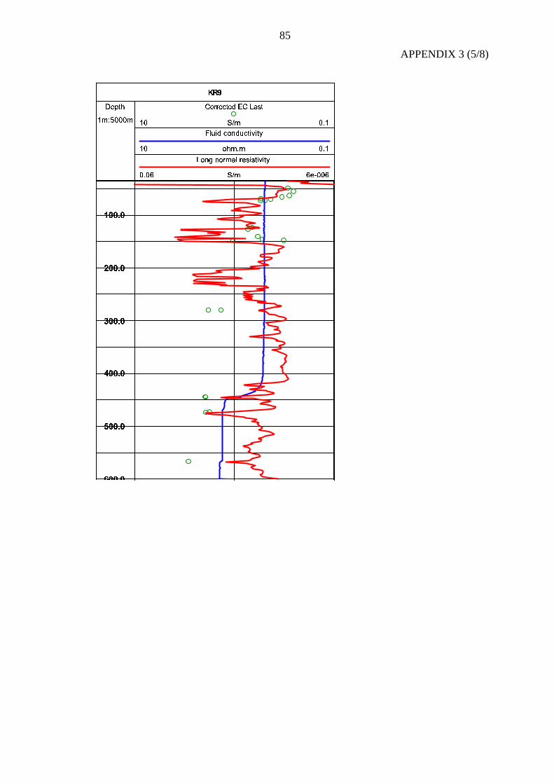
85

APPENDIX 3 (5/8)

" $ &

( ) * + - * + / + 1

" "

- 3 - ) + + / + 1

" 6 6 7 6$ &

8 : ;

< = = > =

? = = > =

A = = > =

B = = > =

C = = > =

D = = =

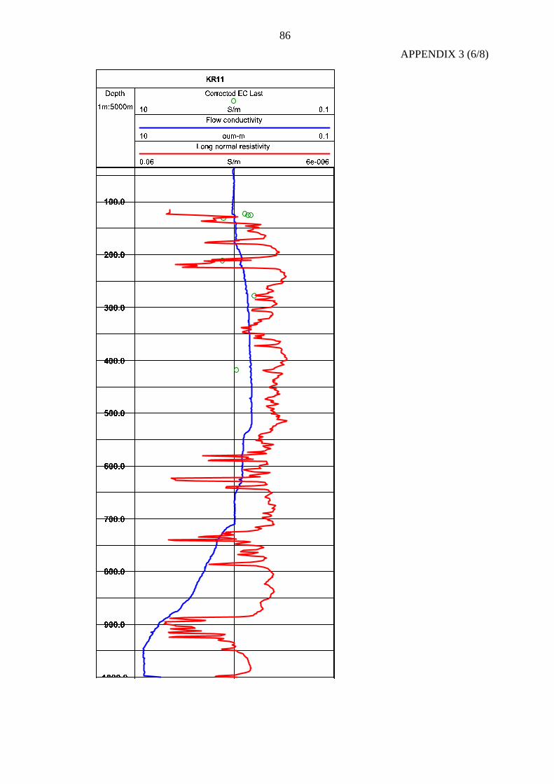
86

APPENDIX 3 (6/8)

" $ &

( ) * + , - . - /

" , 1

+ 4 + ) - - . - /

" 7 7 1 7$ &

9 ; = =

> ? ? @ ?

A ? ? @ ?

C ? ? @ ?

D ? ? @ ?

F ? ? @ ?

G ? ? @ ?

H ? ? @ ?

I ? ? @ ?

J ? ? @ ?

> ? ? ? ?

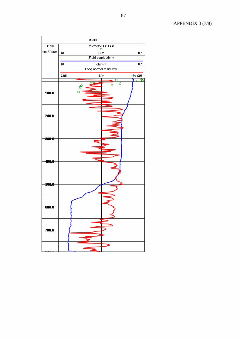
87

APPENDIX 3 (7/8)

" $ &

( ) * + - * + / + 1

" 3

- 6 - ) + + / + 1

" 9 9 3 9$ &

: < > @

A B B C B

D B B C B

F B B C B

G B B C B

I B B C B

J B B C B

K B B C B

L B B B

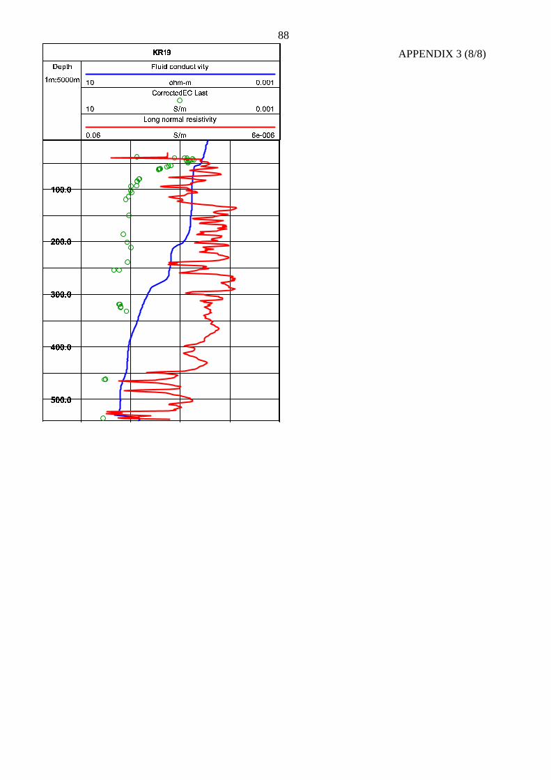
88

APPENDIX 3 (8/8)

" %

' ) ) , ' . / 0

" 1 3

. 4 ) / ) 0 0

" 7 7 % 71 3

8 : < >

? @ @ B @

C @ @ B @

E @ @ B @

F @ @ B @

G @ @ B @

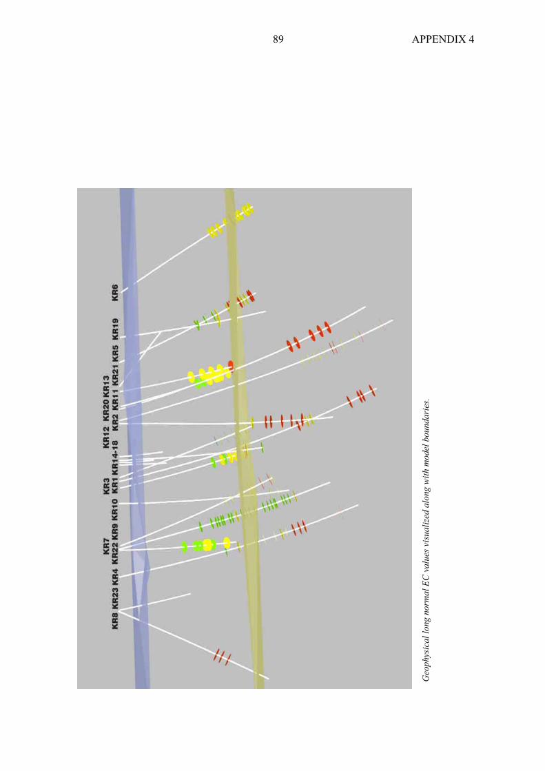
APPENDIX 489

Geo

ph

ysic

al

lon

g n

orm

al

EC

va

lues

vis

ua

lize

d a

lon

g w

ith

mo

del

bo

un

da

ries

.

APPENDIX 490

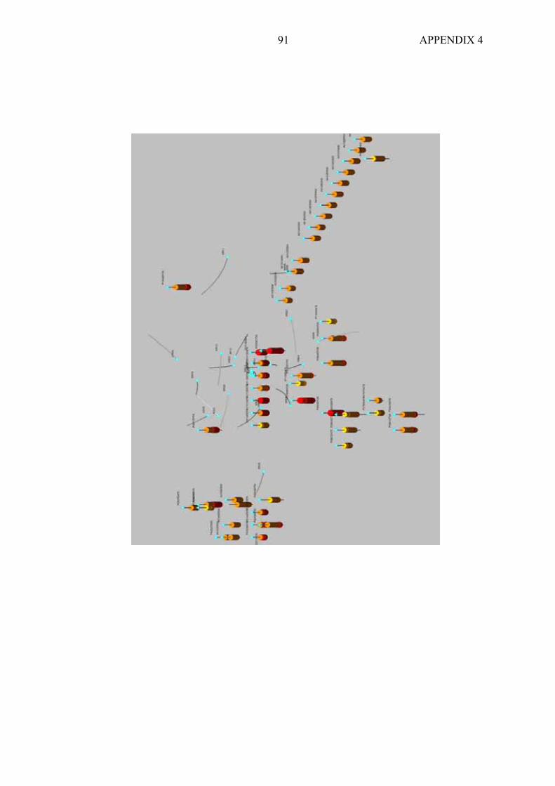
APPENDIX 491

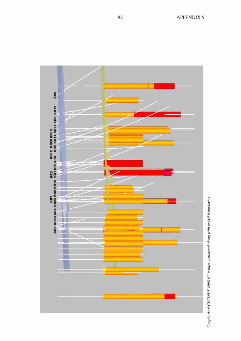
APPENDIX 592

Geo

ph

ysic

al

GE

FIN

EX

40

0S

EC

va

lues

vis

ua

lize

d a

lon

g w

ith

mo

del

bo

un

da

ries

.