Embed Size (px)
Citation preview
3D Human Pose Estimation from a Single Image via Distance Matrix Regression
Francesc Moreno-Noguer
Institut de Robotica i Informatica Industrial (CSIC-UPC), 08028, Barcelona, Spain
Abstract
This paper addresses the problem of 3D human pose esti-
mation from a single image. We follow a standard two-step
pipeline by first detecting the 2D position of the N body
joints, and then using these observations to infer 3D pose.
For the first step, we use a recent CNN-based detector. For
the second step, most existing approaches perform 2N -to-
3N regression of the Cartesian joint coordinates. We show
that more precise pose estimates can be obtained by repre-
senting both the 2D and 3D human poses using N ×N dis-
tance matrices, and formulating the problem as a 2D-to-3Ddistance matrix regression. For learning such a regressor
we leverage on simple Neural Network architectures, which
by construction, enforce positivity and symmetry of the pre-
dicted matrices. The approach has also the advantage to
naturally handle missing observations and allowing to hy-
pothesize the position of non-observed joints. Quantita-
tive results on Humaneva and Human3.6M datasets demon-
strate consistent performance gains over state-of-the-art.
Qualitative evaluation on the images in-the-wild of the LSP
dataset, using the regressor learned on Human3.6M, re-
veals very promising generalization results.
1. Introduction
Estimating 3D human pose from a single RGB image is
known to be a severely ill-posed problem, because many
different body configurations can have virtually the same
projection. A typical solution consists in using discrimi-
native strategies to directly learn mappings from image ev-
idence (e.g. HOG, SIFT) to 3D poses [1, 9, 32, 36, 44].
This has been recently extended to end-to-end mappings us-
ing CNNs [23, 46]. In order to be effective, though, these
approaches require large amounts of training images anno-
tated with the ground truth 3D pose. While obtaining this
kind of data is straightforward for 2D poses, even for im-
ages ‘in the wild’ (e.g. FLIC [35] or LSP [18] datasets), it
requires using sophisticated Motion Capture (MoCap) sys-
tems for the 3D case. Additionally, the datasets acquired
this way (e.g. Humaneva [37], Human3.6M [17]) are mostly
indoors and their images are not representative of the type
of image appearances outside the laboratory.
It seems therefore natural to split the problem in two
stages: Initially use robust image-driven 2D joint detectors,
and then infer the 3D pose from these image observations
using priors learned from MoCap data. This pipeline has
already been used in a number of works [10, 31, 39, 40, 50,
52] and is the strategy we consider in this paper. In partic-
ular, we first estimate 2D joints using a recent CNN detec-
tor [51]. For the second stage, most previous methods per-
form the 2D-to-3D inference in Cartesian space, between
2N - and 3N - vector representations of the N body joints.
In contrast, we propose representing 2D and 3D poses us-
ing N × N matrices of Euclidean distances between every
pair of joints, and formulate the 3D pose estimation prob-
lem as one of 2D-to-3D distance matrix regression1. Fig. 1,
illustrates our pipeline.
Despite being extremely simple to compute, Euclidean
Distance Matrices (EDMs) have several interesting advan-
tages over vector representations that are particularly suited
for our problem. Concretely, EDMs: 1) naturally encode
structural information of the pose. Inference on vector rep-
resentations needs to explicitly formulate such constraints;
2) are invariant to in-plane image rotations and translations,
and normalization operations bring invariance to scaling; 3)
capture pairwise correlations and dependencies between all
body joints.
In order to learn a regression function that maps 2D-to-
3D EDMs we consider Fully Connected (FConn) and Fully
Convolutional (FConv) Network architectures. Since the di-
mension of our data is small (N ×N square matrices, with
N = 14 joints in our model), input-to-output mapping can
be achieved through shallow architectures, with only 2 hid-
den layers for the FConn and 4 convolutional layers for the
FConv. And most importantly, since the distance matrices
used to train the networks are built from solely point con-
figurations, we can easily synthesize artifacts and train the
network under 2D detector noise and body part occlusion.
We achieve state-of-the-art results on standard bench-
marks including Humaneva-I and Human3.6M datasets, and
we show our approach to be robust to large 2D detector er-
1Once the 3D distance matrix is predicted, the position of the 3D body
joints can be estimated using Multidimensional Scaling (MDS).
12823
MDS
Input Image and
2D Detections x
Input 2D EDM
edm(x)
2D-to-3D EDM Regression using a Neural Network
Estimated 3D EDM
edm(y)
Multidimensional Scaling
3D Shape y
Figure 1. Overview. We formulate the 3D human pose estimation problem as a regression between two Euclidean Distance Matrices
(EDMs), encoding pairwise distances of 2D and 3D body joints, respectively. The regression is carried out by a Neural Network, and the
3D joint estimates are obtained from the predicted 3D EDM via Multidimensional Scaling.
rors, while (for the case of the FConv) also allowing to hy-
pothesize reasonably well occluded body limbs. Addition-
ally, experiments in the Leeds Sports Pose dataset, using a
network learned on Human3.6M, demonstrate good gener-
alization capability on images ‘in the wild’.
2. Related Work
Approaches to estimate 3D human pose from single im-
ages can be roughly split into three main categories: meth-
ods that rely on generative models to constrain the space
of possible poses, discriminative approaches that directly
predict 3D pose from image evidence, and methods lying
in-between the two previous categories.
The most straightforward generative model consists in
representing human pose as linear combinations of modes
learned from training data [5]. More sophisticated models
allowing to represent larger deformations include spectral
embedding [43], Gaussian Mixtures on Euclidean or Rie-
mannian manifolds [15, 41] and Gaussian processes [22,
48, 54]. However, exploring the solution space defined
by these generative models requires iterative strategies and
good enough initializations, making these methods more
appropriate for tracking purposes.
Early discriminative approaches [1, 9, 32, 36, 44] fo-
cused on directly predicting 3D pose from image descrip-
tors such as SIFT of HOG filters, and more recently, from
rich features encoding body part information [16] and from
the entire image in Deep architectures [23, 46]. Since
the mapping between feature and pose space is complex
to learn, the success of this family of techniques depends
on the existence of large amounts of training images an-
notated with ground truth 3D poses. Humaneva [37] and
Human3.6M [17] are two popular MoCap datasets used for
this purpose. However, these datasets are acquired in labo-
ratory conditions, preventing the methods that uniquely use
their data to generalize well to unconstrained and realistic
images. [33] addressed this limitation by augmenting the
training data for a CNN with automatically synthesized im-
ages made of realistic textures.
In between the two previous categories, there are a series
of methods that first use discriminative formulations to es-
timate the 2D joint position, and then infer 3D pose using
e.g. regression forests, Expectation Maximization or evolu-
tionary algorithms [10, 26, 31, 39, 40, 50, 52]. The two
steps can be iteratively refined [39, 50, 52] or formulated
independently [10, 26, 31, 40]. By doing this, it is then
possible to exploit the full power of current CNN-based
2D detectors like DeepCut [28] or the Convolutional Pose
Machines (CPMs) [51], which have been trained with large
scale datasets of images ‘in-the-wild’.
Regarding the 3D body pose parameterization, most ap-
proaches use a skeleton with a number N of joints rang-
ing between 14 and 20, and represented by 3N vectors
in a Cartesian space. Very recently, [10] used a gener-
ative volumetric model of the full body. In order to en-
force joint dependency during the 2D-to-3D inference, [17]
and [46] considered latent joint representations, obtained
through Kernel Dependency Estimation and autoencoders.
In this paper, we propose using N ×N Euclidean Distance
Matrices for capturing such joint dependencies.
EDMs have already been used in similar domains, e.g.
in modal analysis to estimate shape basis [2], to represent
protein structures [20], for sensor network localization [7]
and for the resolution of kinematic constraints [29]. It is
worth to point that for 3D shape recognition tasks, Geodesic
Distance Matrices (GDMs) are preferred to EDMs, as they
are invariant to isometric deformations [42]. Yet, for the
same reason, GDMs are not suitable for our problem, be-
cause multiple shape deformations yield the same GDM. In
contrast, the shape that produces a specific EDM is unique
(up to translation, rotation and reflection), and it can be es-
timated via Multidimensional Scaling [7, 11].
Finally, representing 2D and 3D joint positions by dis-
tance matrices, makes it possible to perform inference with
simple Neural Networks. In contrast to recent CNN based
methods for 3D human pose estimation [23, 46] we do not
need to explicitly modify our networks to model the under-
lying joint dependencies. This is directly encoded by the
distance matrices.
2824
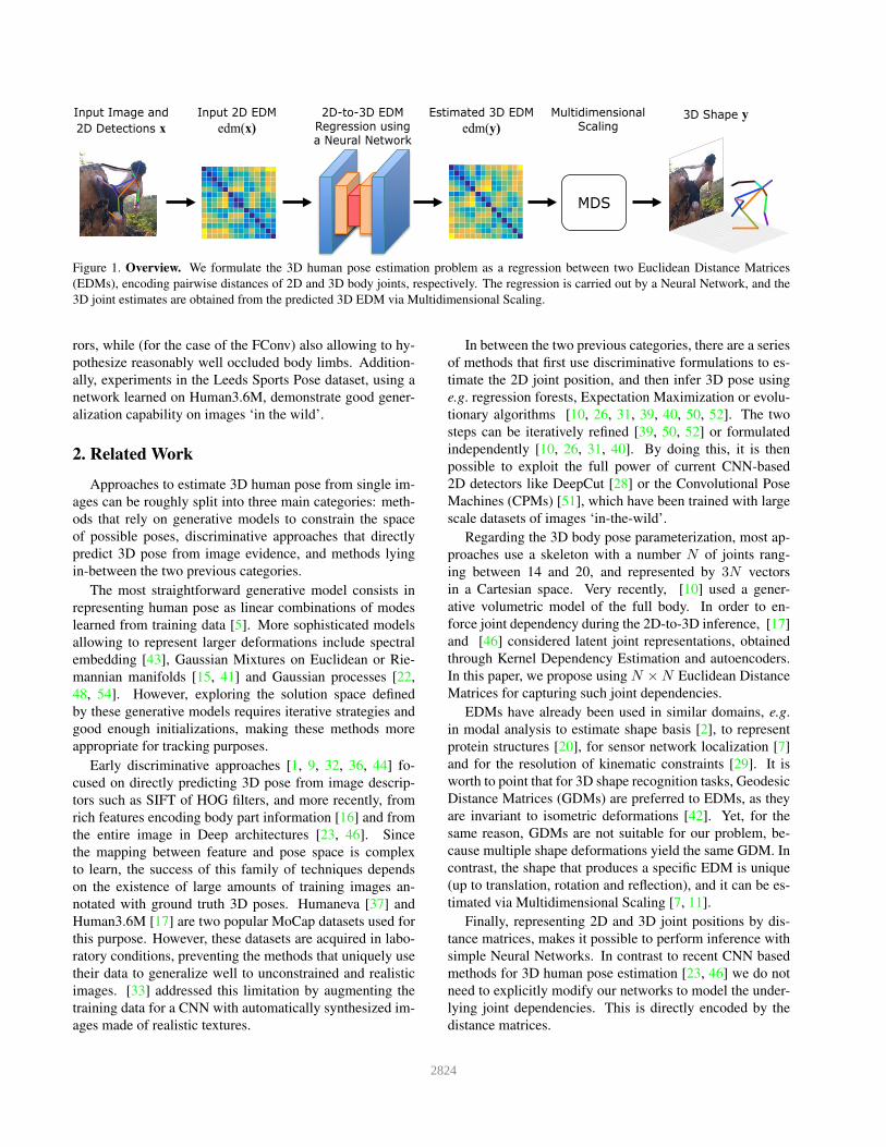
Figure 2. EDMs vs Cartesian representations. Left: Distribution of relative 3D and 2D distances between random pairs of poses, rep-
resented as Cartesian vectors (first plot) and EDM matrices (second plot). Cartesian representations show a more decorrelated pattern
(Pearson correlation coefficient of 0.09 against 0.60 for the EDM), and in particular suffer from larger ambiguities, i.e. poses with similar
2D projections and dissimilar 3D shape. Red circles indicate the most ambiguous such poses, and green circles the most desirable con-
figurations (large 2D and 3D differences). Note that red circles are more uniformly distributed along the vertical axis when using EDM
representations, favoring larger differences and better discriminability. Right: Pairs of dissimilar 3D poses with similar (top) and dissimilar
(bottom) projections. They correspond to the dark red and dark green ‘asterisks’ in the left-most plots.
3. Method
Fig. 1 illustrates the main building blocks of our ap-
proach to estimate 3D human pose from a single RGB im-
age. Given that image, we first detect body joints using
a state-of-the-art detector. Then, 2D joints are normal-
ized and represented by a EDM, which is fed into a Neu-
ral Network to regress a EDM for the 3D body coordi-
nates. Finally, the position of the 3D joints is estimated via
a ‘reflexion-aware’ Multidimensional Scaling approach [7].
We next describe in detail each of these steps.
3.1. Problem Formulation
We represent the 3D pose as a skeleton with N=14 joints
and parameterized by a 3N vector y = [p⊤1, . . . ,p⊤
N ]⊤,
where pi is the 3D location of the i-th joint. Similarly, 2D
poses are represented by 2N vectors x = [u⊤1, . . . ,u⊤
N ]⊤,
where ui are pixel coordinates. Given a full-body person
image, our goal is to estimate the 3D pose vector y. For
this purpose, we follow a regression based discriminative
approach. The most general formulation of this problem
would involve using a set of training images to learn a func-
tion that maps input images, or its features, to 3D poses.
However, as discussed above, such a procedure would re-
quire a vast amount of data to obtain good generalization.
Alternatively, we will first compute the 2D joint position
using the Convolutional Pose Machine detector [51]. We
denote by x the output of the CPM, which is a noisy version
of the ground truth 2D pose x.
We can then formally write our problem as that of learn-
ing a mapping function f : R2N → R3N from potentially
corrupted 2D joint observations x to 3D poses y, given an
annotated and clean training dataset {xi,yi}Di=1
.
3.2. Representing Human Pose with EDMs
In oder to gain depth-scale invariance we first normalize
the vertical coordinates of the projected 2D poses xi to be
within the range [−1, 1]. 3D joint positions yi are expressed
in meters with no further pre-processing. We then represent
both 2D and 3D poses by means of Euclidean Distance Ma-
trices. For the 3D pose y we define edm(y) to be the N×Nmatrix where its (m,n) entry is computed as:
edm(y)m,n = ‖pm − pn‖2 . (1)
Similarly, edm(x) is the N ×N matrix built from the pair-
wise distances between normalized 2D joint coordinates. In
case that some of the joints are occluded, we set to zero their
corresponding rows and columns in edm(x).Despite being simple to define, EDMs have several
advantages over Cartesian representations: EDMs are
coordinate-free, invariant to rotation, translation and reflec-
tion. Previous regression-based approaches [33, 39, 52]
need to compensate for this invariance by pre-aligning the
training 3D poses yi w.r.t. a global coordinate frame, usu-
ally defined by specific body joints. Additionally, EDMs do
not only encode the underlying structure of plain 3D vec-
tor representations, but they also capture richer information
about pairwise correlations between all body joints. A di-
rect consequence of both these advantages, is that EDM-
based representations allow reducing the inherent ambigui-
ties of the 2D-to-3D human pose estimation problem.
To empirically support this claim we randomly picked
pairs of samples from the Humaneva-I dataset and plot-
ted the distribution of relative distances between their
3D and 2D poses, using either Cartesian or EDM
representations (see Fig. 2). For the Cartesian case
(left-most plot), an entry to the graph corresponds to
[dist(yi,yj), dist(xi,xj)], where dist(·) is a normalized
distance and i, j are two random indices. Similarly, for
the EDMs (second plot), an entry to the graph corresponds
to [dist(edm(yi), edm(yj)), dist(edm(xi), edm(xj))]. Ob-
serve that 3D and 2D pairwise differences are much more
correlated in this case. The interpretation of this pattern is
2825
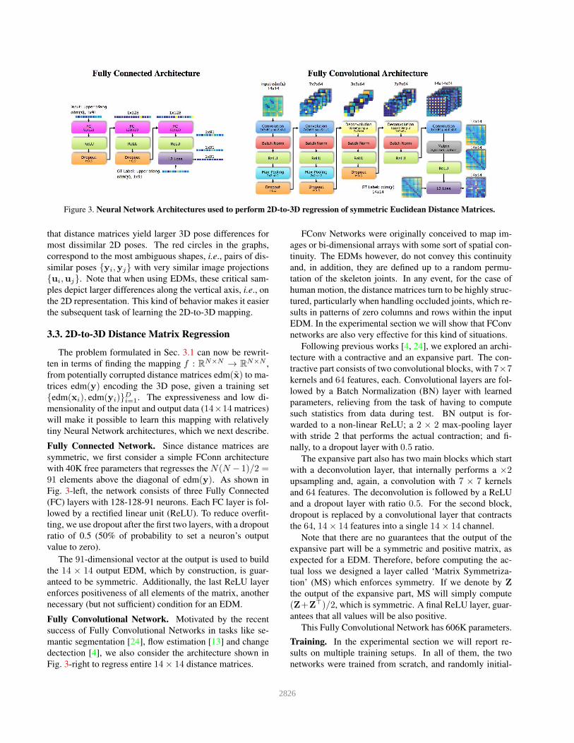
Figure 3. Neural Network Architectures used to perform 2D-to-3D regression of symmetric Euclidean Distance Matrices.
that distance matrices yield larger 3D pose differences for
most dissimilar 2D poses. The red circles in the graphs,
correspond to the most ambiguous shapes, i.e., pairs of dis-
similar poses {yi,yj} with very similar image projections
{ui,uj}. Note that when using EDMs, these critical sam-
ples depict larger differences along the vertical axis, i.e., on
the 2D representation. This kind of behavior makes it easier
the subsequent task of learning the 2D-to-3D mapping.
3.3. 2Dto3D Distance Matrix Regression
The problem formulated in Sec. 3.1 can now be rewrit-
ten in terms of finding the mapping f : RN×N → RN×N ,
from potentially corrupted distance matrices edm(x) to ma-
trices edm(y) encoding the 3D pose, given a training set
{edm(xi), edm(yi)}Di=1
. The expressiveness and low di-
mensionality of the input and output data (14×14 matrices)
will make it possible to learn this mapping with relatively
tiny Neural Network architectures, which we next describe.
Fully Connected Network. Since distance matrices are
symmetric, we first consider a simple FConn architecture
with 40K free parameters that regresses the N(N − 1)/2 =91 elements above the diagonal of edm(y). As shown in
Fig. 3-left, the network consists of three Fully Connected
(FC) layers with 128-128-91 neurons. Each FC layer is fol-
lowed by a rectified linear unit (ReLU). To reduce overfit-
ting, we use dropout after the first two layers, with a dropout
ratio of 0.5 (50% of probability to set a neuron’s output
value to zero).
The 91-dimensional vector at the output is used to build
the 14 × 14 output EDM, which by construction, is guar-
anteed to be symmetric. Additionally, the last ReLU layer
enforces positiveness of all elements of the matrix, another
necessary (but not sufficient) condition for an EDM.
Fully Convolutional Network. Motivated by the recent
success of Fully Convolutional Networks in tasks like se-
mantic segmentation [24], flow estimation [13] and change
dectection [4], we also consider the architecture shown in
Fig. 3-right to regress entire 14× 14 distance matrices.
FConv Networks were originally conceived to map im-
ages or bi-dimensional arrays with some sort of spatial con-
tinuity. The EDMs however, do not convey this continuity
and, in addition, they are defined up to a random permu-
tation of the skeleton joints. In any event, for the case of
human motion, the distance matrices turn to be highly struc-
tured, particularly when handling occluded joints, which re-
sults in patterns of zero columns and rows within the input
EDM. In the experimental section we will show that FConv
networks are also very effective for this kind of situations.
Following previous works [4, 24], we explored an archi-
tecture with a contractive and an expansive part. The con-
tractive part consists of two convolutional blocks, with 7×7kernels and 64 features, each. Convolutional layers are fol-
lowed by a Batch Normalization (BN) layer with learned
parameters, relieving from the task of having to compute
such statistics from data during test. BN output is for-
warded to a non-linear ReLU; a 2 × 2 max-pooling layer
with stride 2 that performs the actual contraction; and fi-
nally, to a dropout layer with 0.5 ratio.
The expansive part also has two main blocks which start
with a deconvolution layer, that internally performs a ×2upsampling and, again, a convolution with 7 × 7 kernels
and 64 features. The deconvolution is followed by a ReLU
and a dropout layer with ratio 0.5. For the second block,
dropout is replaced by a convolutional layer that contracts
the 64, 14× 14 features into a single 14× 14 channel.
Note that there are no guarantees that the output of the
expansive part will be a symmetric and positive matrix, as
expected for a EDM. Therefore, before computing the ac-
tual loss we designed a layer called ‘Matrix Symmetriza-
tion’ (MS) which enforces symmetry. If we denote by Z
the output of the expansive part, MS will simply compute
(Z+Z⊤)/2, which is symmetric. A final ReLU layer, guar-
antees that all values will be also positive.
This Fully Convolutional Network has 606K parameters.
Training. In the experimental section we will report re-
sults on multiple training setups. In all of them, the two
networks were trained from scratch, and randomly initial-
2826
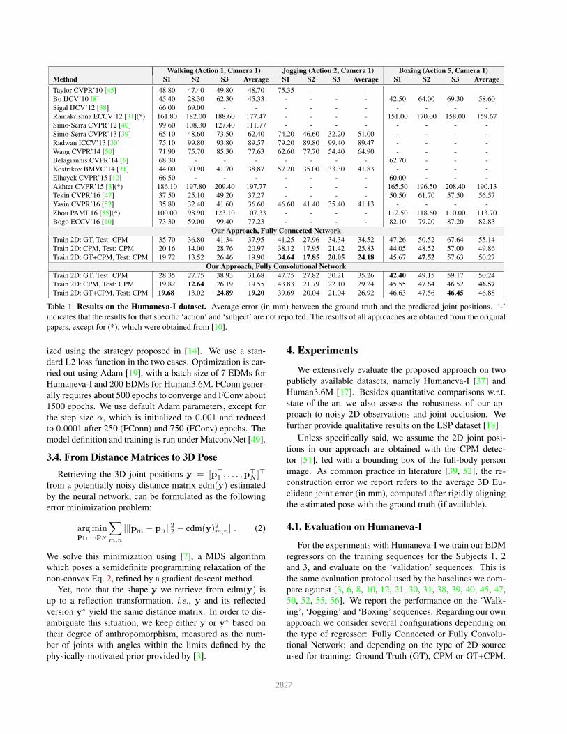
Walking (Action 1, Camera 1) Jogging (Action 2, Camera 1) Boxing (Action 5, Camera 1)
Method S1 S2 S3 Average S1 S2 S3 Average S1 S2 S3 Average
Taylor CVPR’10 [45] 48.80 47.40 49.80 48,70 75,35 - - - - - - -
Bo IJCV’10 [8] 45.40 28.30 62.30 45.33 - - - - 42.50 64.00 69.30 58.60
Sigal IJCV’12 [38] 66.00 69.00 - - - - - - - - - -
Ramakrishna ECCV’12 [31](*) 161.80 182.00 188.60 177.47 - - - - 151.00 170.00 158.00 159.67
Simo-Serra CVPR’12 [40] 99.60 108.30 127.40 111.77 - - - - - - - -
Simo-Serra CVPR’13 [39] 65.10 48.60 73.50 62.40 74.20 46.60 32.20 51.00 - - - -
Radwan ICCV’13 [30] 75.10 99.80 93.80 89.57 79.20 89.80 99.40 89.47 - - - -
Wang CVPR’14 [50] 71.90 75.70 85.30 77.63 62.60 77.70 54.40 64.90 - - - -
Belagiannis CVPR’14 [6] 68.30 - - - - - - - 62.70 - - -
Kostrikov BMVC’14 [21] 44.00 30.90 41.70 38,87 57.20 35.00 33.30 41.83 - - - -
Elhayek CVPR’15 [12] 66.50 - - - - - - - 60.00 - - -
Akhter CVPR’15 [3](*) 186.10 197.80 209.40 197.77 - - - - 165.50 196.50 208.40 190.13
Tekin CVPR’16 [47] 37.50 25.10 49.20 37.27 - - - - 50.50 61.70 57.50 56.57
Yasin CVPR’16 [52] 35.80 32.40 41.60 36.60 46.60 41.40 35.40 41.13 - - - -
Zhou PAMI’16 [55](*) 100.00 98.90 123.10 107.33 - - - - 112.50 118.60 110.00 113.70
Bogo ECCV’16 [10] 73.30 59.00 99.40 77.23 - - - - 82.10 79.20 87.20 82.83
Our Approach, Fully Connected Network
Train 2D: GT, Test: CPM 35.70 36.80 41.34 37.95 41.25 27.96 34.34 34.52 47.26 50.52 67.64 55.14
Train 2D: CPM, Test: CPM 20.16 14.00 28.76 20.97 38.12 17.95 21.42 25.83 44.05 48.52 57.00 49.86
Train 2D: GT+CPM, Test: CPM 19.72 13.52 26.46 19.90 34.64 17.85 20.05 24.18 45.67 47.52 57.63 50.27
Our Approach, Fully Convolutional Network
Train 2D: GT, Test: CPM 28.35 27.75 38.93 31.68 47.75 27.82 30.21 35.26 42.40 49.15 59.17 50.24
Train 2D: CPM, Test: CPM 19.82 12.64 26.19 19.55 43.83 21.79 22.10 29.24 45.55 47.64 46.52 46.57
Train 2D: GT+CPM, Test: CPM 19.68 13.02 24.89 19.20 39.69 20.04 21.04 26.92 46.63 47.56 46.45 46.88
Table 1. Results on the Humaneva-I dataset. Average error (in mm) between the ground truth and the predicted joint positions. ‘-’
indicates that the results for that specific ‘action’ and ‘subject’ are not reported. The results of all approaches are obtained from the original
papers, except for (*), which were obtained from [10].
ized using the strategy proposed in [14]. We use a stan-
dard L2 loss function in the two cases. Optimization is car-
ried out using Adam [19], with a batch size of 7 EDMs for
Humaneva-I and 200 EDMs for Human3.6M. FConn gener-
ally requires about 500 epochs to converge and FConv about
1500 epochs. We use default Adam parameters, except for
the step size α, which is initialized to 0.001 and reduced
to 0.0001 after 250 (FConn) and 750 (FConv) epochs. The
model definition and training is run under MatconvNet [49].
3.4. From Distance Matrices to 3D Pose
Retrieving the 3D joint positions y = [p⊤1, . . . ,p⊤
N ]⊤
from a potentially noisy distance matrix edm(y) estimated
by the neural network, can be formulated as the following
error minimization problem:
argminp1,...,pN
∑
m,n
|‖pm − pn‖2
2− edm(y)2m,n| . (2)
We solve this minimization using [7], a MDS algorithm
which poses a semidefinite programming relaxation of the
non-convex Eq. 2, refined by a gradient descent method.
Yet, note that the shape y we retrieve from edm(y) is
up to a reflection transformation, i.e., y and its reflected
version y∗ yield the same distance matrix. In order to dis-
ambiguate this situation, we keep either y or y∗ based on
their degree of anthropomorphism, measured as the num-
ber of joints with angles within the limits defined by the
physically-motivated prior provided by [3].
4. Experiments
We extensively evaluate the proposed approach on two
publicly available datasets, namely Humaneva-I [37] and
Human3.6M [17]. Besides quantitative comparisons w.r.t.
state-of-the-art we also assess the robustness of our ap-
proach to noisy 2D observations and joint occlusion. We
further provide qualitative results on the LSP dataset [18]
Unless specifically said, we assume the 2D joint posi-
tions in our approach are obtained with the CPM detec-
tor [51], fed with a bounding box of the full-body person
image. As common practice in literature [39, 52], the re-
construction error we report refers to the average 3D Eu-
clidean joint error (in mm), computed after rigidly aligning
the estimated pose with the ground truth (if available).
4.1. Evaluation on HumanevaI
For the experiments with Humaneva-I we train our EDM
regressors on the training sequences for the Subjects 1, 2
and 3, and evaluate on the ‘validation’ sequences. This is
the same evaluation protocol used by the baselines we com-
pare against [3, 6, 8, 10, 12, 21, 30, 31, 38, 39, 40, 45, 47,
50, 52, 55, 56]. We report the performance on the ‘Walk-
ing’, ‘Jogging’ and ‘Boxing’ sequences. Regarding our own
approach we consider several configurations depending on
the type of regressor: Fully Connected or Fully Convolu-
tional Network; and depending on the type of 2D source
used for training: Ground Truth (GT), CPM or GT+CPM.
2827
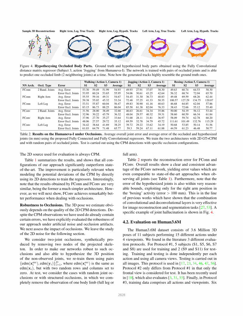
Sample 3D Reconstructions Right Arm, Leg, True Tracks Right Arm, Leg, Hypoth. Tracks Left Arm, Leg, True Tracks Left Arm, Leg, Hypoth. Tracks
Figure 4. Hypothesysing Occluded Body Parts. Ground truth and hypothesized body parts obtained using the Fully Convolutional
distance matrix regressor (Subject 3, action ‘Jogging’ from Humaneva-I). The network is trained with pairs of occluded joints and is able
to predict one occluded limb (2 neighboring joints) at a time. Note how the generated tracks highly resemble the ground truth ones.
Walking (Action 1, Camera 1) Jogging (Action 2, Camera 1) Boxing (Action 5, Camera 1)
NN Arch. Occl. Type Error S1 S2 S3 Average S1 S2 S3 Average S1 S2 S3 Average
FConn 2 Rand. Joints Avg. Error 53.30 59.49 51.99 54.93 49.93 27.91 37.07 38.30 49.63 60.74 64.53 58.30
Error Occl. Joints 53.95 60.24 53.65 55.95 54.06 30.61 43.25 42.64 56.32 68.74 72.04 65.70
FConn Right Arm Avg. Error 55.55 59.16 49.31 54.67 54.45 31.30 36.73 40.83 49.48 69.59 68.26 62.44
Error Occl. Joints 59.38 55.02 45.32 53.24 72.48 37.25 41.33 50.35 100.57 127.29 134.75 120.87
FConn Left Leg Avg. Error 53.51 55.87 60.04 56.47 49.83 30.90 41.16 40.63 46.68 64.85 62.04 57.86
Error Occl. Joints 83.15 86.73 88.25 86.04 85.58 61.38 82.04 76.33 38.43 72.66 55.12 55.40
FConv 2 Rand. Joints Avg. Error 31.56 28.00 38.49 32.68 46.63 26.61 34.34 35.86 50.00 54.19 56.12 53.44
Error Occl. Joints 32.96 30.22 45.79 36.32 48.04 29.57 40.32 39.31 58.60 60.59 66.34 61.84
FConv Right Arm Avg. Error 37.96 27.70 35.27 33.64 51.00 28.11 31.81 36.97 58.09 59.74 62.78 60.20
Error Occl. Joints 48.06 27.57 29.72 35.12 69.59 32.78 34.79 45.72 111.61 101.49 132.76 115.29
FConv Left Leg Avg. Error 34.42 38.64 41.69 38.25 39.72 29.22 33.62 34.19 50.68 53.85 50.14 51.56
Error Occl. Joints 61.03 64.79 71.48 65.77 59.3 59.24 67.11 61.88 44.59 61.23 46.48 50.77
Table 2. Results on the Humaneva-I under Occlusions. Average overall joint error and average error of the occluded and hypothesized
joints (in mm) using the proposed Fully Connected and Fully Convolutional regressors. We train the two architectures with 2D GT+CPM
and with random pairs of occluded joints. Test is carried out using the CPM detections with specific occlusion configurations.
The 2D source used for evaluation is always CPM.
Table 1 summarizes the results, and shows that all con-
figurations of our approach significantly outperform state-
of-the-art. The improvement is particularly relevant when
modeling the potential deviations of the CPM by directly
using its 2D detections to train the regressors. Interestingly,
note that the results obtained by FConn and FConv are very
similar, being the former a much simpler architecture. How-
ever, as we will next show, FConv achieves remarkably bet-
ter performance when dealing with occlusions.
Robustness to Occlusions. The 3D pose we estimate obvi-
ously depends on the quality of the 2D CPM detections. De-
spite the CPM observations we have used do already contain
certain errors, we have explicitly evaluated the robustness of
our approach under artificial noise and occlusion artifacts.
We next assess the impact of occlusions. We leave the study
of the 2D noise for the following section.
We consider two-joint occlusions, synthetically pro-
duced by removing two nodes of the projected skele-
ton. In order to make our networks robust to such oc-
clusions and also able to hypothesize the 3D position
of the non-observed joints, we re-train them using pairs
{edm(xocci ), edm(yi)}
Di=1
, where edm(xocci ) is the same as
edm(xi), but with two random rows and columns set to
zero. At test, we consider the cases with random joint oc-
clusions or with structured occlusions, in which we com-
pletely remove the observation of one body limb (full leg or
full arm).
Table 2 reports the reconstruction error for FConn and
FConv. Overall results show a clear and consistent advan-
tage of the FConv network, yielding error values which are
even comparable to state-of-the-art approaches when ob-
serving all joints (see Table 1). Furthermore, note that the
error of the hypothesized joints is also within very reason-
able bounds, exploiting only for the right arm position in
the ‘boxing’ activity (error > 100 mm). This is in the line
of previous works which have shown that the combination
of convolutional and deconvolutional layers is very effective
for image reconstruction and segmentation tasks [27, 53]. A
specific example of joint hallucination is shown in Fig. 4.
4.2. Evaluation on Human3.6M
The Human3.6M dataset consists of 3.6 Million 3D
poses of 11 subjects performing 15 different actions under
4 viewpoints. We found in the literature 3 different evalua-
tion protocols. For Protocol #1, 5 subjects (S1, S5, S6, S7
and S8) are used for training and 2 (S9 and S11) for test-
ing. Training and testing is done independently per each
action and using all camera views. Testing is carried out in
all images. This protocol is used in [17, 23, 34, 46, 47, 56].
Protocol #2 only differs from Protocol #1 in that only the
frontal view is considered for test. It has been recently used
in [10], which also evaluates [3, 31, 55]. Finally, in Protocol
#3, training data comprises all actions and viewpoints. Six
2828

Method Direct. Discuss Eat Greet Phone Pose Purch. Sit SitD Smoke Photo Wait Walk WalkD WalkT Avg
Protocol #1
Ionescu PAMI’14 [17] 132.71 183.55 133.37 164.39 162.12 205.94 150.61 171.31 151.57 243.03 162.14 170.69 177.13 96.60 127.88 162,20
Li ICCV’15 [23] - 136.88 96.94 124.74 - 168.08 - - - - - - 132.17 69.97 - -
Tekin BMVC’16 [46] - 129.06 91.43 121.68 - - - - - - 162.17 - 65.75 130.53 - -
Tekin CVPR’16 [47] 102.41 147.72 88.83 125.28 118.02 112.38 129.17 138.89 224.90 118.42 182.73 138.75 55.07 126.29 65.76 124.97
Zhou CVPR’16 [56] 87.36 109.31 87.05 103.16 116.18 143.32 106.88 99.78 124.52 199.23 107.42 118.09 114.23 79.39 97.70 112.91
Sanzari ECCV’16 [34] 48.82 56.31 95.98 84.78 96.47 66.30 107.41 116.89 129.63 97.84 105.58 65.94 92.58 130.46 102.21 93.15
Ours, FConv, Test 2D: CPM 67.48 79.01 76.48 83.12 97.43 74.58 71.96 102.40 116.68 87.70 100.37 94.57 75.21 82.72 74.92 85.64
Protocol #2
Ramakrishna ECCV’12 [31](*) 137.40 149.30 141.60 154.30 157.70 141.80 158.10 168.60 175.60 160.40 158.90 161.70 174.80 150.00 150.20 156.03
Akhter CVPR’15 [3](*) 1199.20 177.60 161.80 197.80 176.20 195.40 167.30 160.70 173.70 177.80 186.50 181.90 198.60 176.20 192.70 181.56
Zhou PAMI’16 [55](*) 99.70 95.80 87.90 116.80 108.30 93.50 95.30 109.10 137.50 106.00 107.30 102.20 110.40 106.50 115.20 106.10
Bogo ECCV’16 [10] 62.00 60.20 67.80 76.50 92.10 73.00 75.30 100.30 137.30 83.40 77.00 77.30 86.80 79.70 81.70 82.03
Ours. FConv, Test 2D: CPM 64.11 76.58 70.59 80.81 93.01 74.01 65.45 87.93 109.49 83.81 96.31 93.08 73.51 81.57 72.59 81.52
Protocol #3
Yasin CVPR’16 [52] 88.40 72.50 108.50 110.20 97.10 81.60 107.20 119.00 170.80 108.20 142.50 86.90 92.10 165.70 102.00 110.18
Rogez NIPS’16 [33] - - - - - - - - - - - - - - - 88.10
Ours, FConv, Test 2D: CPM 66.05 61.69 84.51 73.73 65.23 67.17 60.85 67.29 103.48 74.75 92.55 69.59 71.47 78.04 73.23 73.98
Table 3. Results on the Human3.6M dataset. Average joint error (in mm) considering the 3 evaluation prototocols described in the text.
The results of all approaches are obtained from the original papers, except for (*), which are from [10].
Occ. Type Error Direct. Discuss Eat Greet Phone Pose Purch. Sit SitD Smoke Photo Wait Walk WalkD WalkT Avg
2 Rnd.Joints Avg. Error 88.53 97.83 139.99 99.57 106.13 102.78 92.97 113.35 126.62 111.73 122.74 109.85 95.1 96.76 97.97 106.79
Err.Occl. Joints 94.77 104.37 155.66 110.48 119.62 103.83 91.04 141.31 135.35 137.76 146.68 131.41 116.16 96.11 99.73 118.95
Left Arm Avg. Error 197.86 101.88 123.91 109.72 93.00 106.15 100.55 113.19 129.50 111.15 135.72 118.07 99.21 100.73 100.94 109.44
Err.Occl. Joints 177.44 177.68 152.06 220.28 145.93 180.42 143.24 192.42 154.62 184.24 253.88 213.6 176.11 160.44 188.38 181.38
Right Leg Avg. Error 79.94 82.23 132.64 92.05 100.77 97.32 76.37 126.95 125.51 106.66 109.82 95.92 94.88 89.82 91.60 100.17
Err.Occl. Joints 81.23 92.57 177.80 103.69 148.45 120.74 92.63 200.56 183.03 146.10 145.29 107.36 133.11 105.9 120.12 130.57
Table 4. Results on Human3.6M under Occlusions. Average overall joint error and average error of the hypothesized occluded joints (in
mm). The network is trained and evaluated according to the ‘Protocol #3’ described in the text.
2D Input Direct. Discuss Eat Greet Phone Pose Purch. Sit SitD Smoke Photo Wait Walk WalkD WalkT Avg
GT 53.51 50.52 65.76 62.47 56.9 60.63 50.83 55.95 79.62 63.68 80.83 61.80 59.42 68.53 62.11 62.17
GT+N (0, 5) 57.05 56.05 70.33 65.46 60.39 64.49 59.06 58.62 82.80 67.85 83.97 70.13 66.76 75.04 68.62 67.11
GT+N (0, 10) 76.46 70.74 77.18 77.25 73.42 81.94 64.65 71.05 97.08 76.91 93.45 77.12 85.14 80.96 83.47 79.12
GT+N (0, 15) 90.72 91.99 96.54 94.99 87.43 101.81 89.39 84.46 107.26 93.31 106.01 95.96 100.38 96.59 104.41 96.08
GT+N (0, 20) 109.84 110.21 117.13 115.16 107.08 116.92 107.14 101.82 131.43 114.76 115.07 112.54 125.50 118.93 129.73 115.55
Table 5. Results on the Human3.6M dataset under 2D Noise. Average 3D joint error for increasing levels of 2D noise. The network is
trained with 2D Ground Truth (GT) data and evaluated with GT+N (0.σ). where σ is the standard deviation (in pixels) of the noise.
subjects (S1, S5, S6, S7, S8 and S9) are used for training
and every 64th frame of the frontal view of S11 is used for
testing. This is the protocol considered in [33, 52].
We will evaluate our approach on the three protocols.
In contrast to HumanEva experiments, CPM detections will
not be used for training (very time consuming), and we will
train with the ground truth 2D positions. CPM detections
are used during test, though. For Protocol #3 we choose the
training set by randomly picking 400K samples among all
poses and camera views, a similar number as in [52]. For the
rest of experiments we will only consider the FConv regres-
sor, which showed overall better performance than FConn
in the Humaneva dataset. The results are summarized in
Table 3. For Protocols #1 and #3 our approach improves
state-of-the-art by a considerable margin, and for Protocol
#2 is very similar to [10], a recent approach that relies on a
high-quality volumetric prior of the body shape.
Robustness to Occlusions. We perform the same occlu-
sion analysis as we did for Humaneva-I and re-train the net-
work under randomly occluded joints and test for random
and structured occlusions. The results (under Protocol #3)
are reported in Table 4. Again, note that the average body
error remains within reasonable bounds. There are, how-
ever, some specific actions (e.g. ‘Sit’, ‘Photo’) for which
the occluded leg or arm are not very well hypothesized. We
believe this is because in these actions, the limbs are in con-
figurations with only a few samples on the training set. In-
deed, state of the art methods also report poor performance
on these actions, even when observing all joints.
Robustness to 2D Noise. We further analyze the robustness
of our approach (trained on clean data) to 2D noise. For this
purpose, instead of using CPM detections for test, we used
the 2D ground truth test poses with increasing amounts of
Gaussian noise. The results of this analysis are given in
Table 5. Note that the 3D error gradually increases with the
2D noise, but does not seem to break the system. Noise
levels of up to 20 pixels std are still reasonably supported.
As a reference, the mean 2D error of the CPM detections
considered in Tables 4 and 3 is of 10.91 pixels. Note also
that there is still room for improvement, as more precise 2D
detections can considerably boost the 3D pose accuracy.
4.3. Evaluation on Leeds Sports Pose Dataset
We finally explore the generalization capabilities of our
approach on the LSP dataset. For each input image, we
locate the 2D joints using the CPM detector, perform the
2829
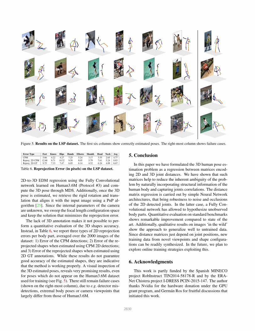
Figure 5. Results on the LSP dataset. The first six columns show correctly estimated poses. The right-most column shows failure cases.
Error Type Feet Knees Hips Hands Elbows Should. Head Neck Avg
CPM 5.66 4.22 4.27 7.25 5.24 3.17 3.55 2.65 4.77
Reproj. 2D CPM 12.68 8.71 10.32 9.50 8.05 5.79 7.61 5.24 8.83
Reproj. 2D GT 9.75 7.33 7.47 6.05 6.14 4.52 6.24 4.09 6.67
Table 6. Reprojection Error (in pixels) on the LSP dataset.
2D-to-3D EDM regression using the Fully Convolutional
network learned on Human3.6M (Protocol #3) and com-
pute the 3D pose through MDS. Additionally, once the 3D
pose is estimated, we retrieve the rigid rotation and trans-
lation that aligns it with the input image using a PnP al-
gorithm [25]. Since the internal parameters of the camera
are unknown, we sweep the focal length configuration space
and keep the solution that minimizes the reprojection error.
The lack of 3D annotation makes it not possible to per-
form a quantitative evaluation of the 3D shapes accuracy.
Instead, in Table 6, we report three types of 2D reprojection
errors per body part, averaged over the 2000 images of the
dataset: 1) Error of the CPM detections; 2) Error of the re-
projected shapes when estimated using CPM 2D detections;
and 3) Error of the reprojected shapes when estimated using
2D GT annotations. While these results do not guarantee
good accuracy of the estimated shapes, they are indicative
that the method is working properly. A visual inspection of
the 3D estimated poses, reveals very promising results, even
for poses which do not appear on the Human3.6M dataset
used for training (see Fig. 5). There still remain failure cases
(shown on the right-most column), due to e.g. detector mis-
detections, extremal body poses or camera viewpoints that
largely differ from those of Human3.6M.
5. Conclusion
In this paper we have formulated the 3D human pose es-
timation problem as a regression between matrices encod-
ing 2D and 3D joint distances. We have shown that such
matrices help to reduce the inherent ambiguity of the prob-
lem by naturally incorporating structural information of the
human body and capturing joints correlations. The distance
matrix regression is carried out by simple Neural Network
architectures, that bring robustness to noise and occlusions
of the 2D detected joints. In the latter case, a Fully Con-
volutional network has allowed to hypothesize unobserved
body parts. Quantitative evaluation on standard benchmarks
shows remarkable improvement compared to state of the
art. Additionally, qualitative results on images ‘in the wild’
show the approach to generalize well to untrained data.
Since distance matrices just depend on joint positions, new
training data from novel viewpoints and shape configura-
tions can be readily synthesized. In the future, we plan to
explore online training strategies exploiting this.
6. Acknowledgments
This work is partly funded by the Spanish MINECO
project RobInstruct TIN2014-58178-R and by the ERA-
Net Chistera project I-DRESS PCIN-2015-147. The author
thanks Nvidia for the hardware donation under the GPU
grant program, and German Ros for fruitful discussions that
initiated this work.
2830

References
[1] A. Agarwal and B. Triggs. 3D Human Pose from Silhouettes
by Relevance Vector Regression. In Conference on Com-
puter Vision and Pattern Recognition. 1, 2
[2] A. Agudo, J. M. M. Montiel, B. Calvo, and F. Moreno-
Noguer. Mode-Shape Interpretation: Re-Thinking Modal
Space for Recovering Deformable Shapes. In Winter Con-
ference on Applications of Computer Vision, 2016. 2
[3] I. Akhter and M. Black. Pose-conditioned Joint Angle Lim-
its for 3D Human Pose Reconstruction. In Conference on
Computer Vision and Pattern Recognition, 2015. 5, 6, 7
[4] P. F. Alcantarilla, S. Stent, G. Ros, R. Arroyo, and R. Gher-
ardi. Street-View Change Detection with Deconvolutional
Networks. In Robotics: Science and Systems Conference,
2016. 4
[5] A. O. Balan, L. Sigal, M. J. Black, J. E. Davis, and H. W.
Haussecker. Detailed Human Shape and Pose from Images.
In Conference on Computer Vision and Pattern Recognition,
2007. 2
[6] V. Belagiannis, S. Amin, M. Andriluka, B. S. N. Navab, and
S. Ilic. 3D Pictorial Structures for Multiple Human Pose
Estimation. In Conference on Computer Vision and Pattern
Recognition, 2014. 5
[7] P. Biswas, T. Liang, K. Toh, T. Wang, and Y. Ye. Semidefi-
nite Programming Approaches for Sensor Network Localiza-
tion With Noisy Distance Measurements. IEEE Transactions
on Automation Science and Engineering, 3:360–371, 2006.
2, 3, 5
[8] L. Bo and C. Sminchisescu. Twin Gaussian Processes for
Structured Prediction. International Journal of Computer Vi-
sion, 87:28–52, 2010. 5
[9] L. Bo, C. Sminchisescu, A. Kanaujia, and D. Metaxas. Fast
Algorithms for Large Scale Conditional 3D Prediction. In
Conference on Computer Vision and Pattern Recognition,
2008. 1, 2
[10] F. Bogo, A. Kanazawa, C. Lassner, P. Gehler, J. Romero, and
M. J. Black. Keep it SMPL: Automatic Estimation of 3D
Human Pose and Shape from a Single Image. In European
Conference on Computer Vision, 2016. 1, 2, 5, 6, 7
[11] I. Borg and P. Groenen. Modern Multidimensional Scaling:
Theory and Applications. Springer, 2005. 2
[12] A. Elhayek, E. Aguiar, A. Jain, J. Tompson, L. Pishchulin,
M. Andriluka, C. Bregler, B. Schiele, and C. Theobalt. Ef-
ficient Convnet-Based Marker-Less Motion Capture in Gen-
eral Scenes with a Low Number of Cameras. In Conference
on Computer Vision and Pattern Recognition, 2015. 5
[13] P. Fischer, A. Dosovitskiy, E. Ilg, C. H. P. Hausser,
V. Golkov, P. v.d. Smagt, D. Cremers, and T. Brox. FlowNet:
Learning Optical Flow with Convolutional Networks. In In-
ternational Conference on Computer Vision, 2015. 4
[14] K. He, X. Zhang, S. Ren, and J. Sun. Delving Deep into Rec-
tifiers: Surpassing Human-Level Performance on ImageNet
Classification. In International Conference on Computer Vi-
sion, 2015. 5
[15] N. R. Howe, M. E. Leventon, and W. T. Freeman. Bayesian
Reconstruction of 3D Human Motion from Single-Camera
Video. In Neural Information Processing Systems, 1999. 2
[16] C. Ionescu, J. Carreira, and C. Sminchisescu. Iterated
Second-Order Label Sensitive Pooling for 3D Human Pose.
In Conference on Computer Vision and Pattern Recognition,
2014. 2
[17] C. Ionescu, D. Papava, V. Olaru, and C. Sminchisescu.
Human3.6M: Large Scale Datasets and Predictive Methods
for 3D Human Sensing in Natural Environments. IEEE
Transactions on Pattern Analysis and Machine Intelligence,
36(7):1325–1339, 2014. 1, 2, 5, 6, 7
[18] S. Johnson and M. Everingham. Clustered Pose and Non-
linear Appearance Models for Human Pose Estimation. In
British Machine Vision Conference, 2010. 1, 5
[19] P. Kingma and J. Ba. Adam: A Method for Stochastic Op-
timization. In International Conference in Learning Repre-
sentations, 2015. 5
[20] A. Kloczkowski, R. L. Jernigan, Z. Wu, G. Song, L. Yang,
A. Kolinski, and P. Pokarowski. Distance Matrix-based Ap-
proach to Protein Structure Prediction. Journal of Structural
and Functional Genomics, 10(1):67–81, 2009. 2
[21] I. Kostrikov and J. Gall. Depth Sweep Regression Forests for
Estimating 3D Human Pose from Images. In British Machine
Vision Conference, 2014. 5
[22] N. D. Lawrence and A. J. Moore. Hierarchical Gaussian Pro-
cess Latent Variable Models. In International Conference in
Machine Learning, 2007. 2
[23] S. Li, W. Zhang, and A. Chan. Maximum-Margin Structured
Learning with Deep Networks for 3D Human Pose Estima-
tion. In International Conference on Computer Vision, 2015.
1, 2, 6, 7
[24] J. Long, E. Shelhamer, and T. Darrell. Fully convolutional
networks for semantic segmentation. In Conference on Com-
puter Vision and Pattern Recognition, 2015. 4
[25] C.-P. Lu, G. D. Hager, and E. Mjolsness. Fast and Glob-
ally Convergent Pose Estimation from Video Images. IEEE
Transactions on Pattern Analysis and Machine Intelligence,
22(5):610–622, 2000. 8
[26] G. Mori and J. Malik. Recovering 3D Human Body Configu-
rations Using Shape Contexts. IEEE Transactions on Pattern
Analysis and Machine Intelligence, 28:1052–1062, 2006. 2
[27] H. Noh, S. Hong, and B. Han. Learning deconvolution net-
work for semantic segmentation. In International Confer-
ence on Computer Vision, 2015. 6
[28] L. Pishchulin, E. Insafutdinov, S. Tang, B. Andres, M. An-
driluka, P. Gehler, and B. Schiele. Deepcut: Joint subset par-
tition and labeling for multi person pose estimation. In Con-
ference on Computer Vision and Pattern Recognition, 2016.
2
[29] J. Porta, L. Ros, F. Thomas, and C. Torras. A Branch-and-
Prune Solver for Distance Constraints. IEEE Transactions
on Robotics, 21:176–187, 2005. 2
[30] I. Radwan, A. Dhall, and R. Goecke. Monocular Image 3D
Human Pose Estimation Under Self-Occlusion. In Interna-
tional Conference on Computer Vision, 2013. 5
[31] V. Ramakrishna, T. Kanade, and Y. A. Sheikh. Reconstruct-
ing 3D Human Pose from 2D Image Landmarks. In Euro-
pean Conference on Computer Vision, 2012. 1, 2, 5, 6, 7
2831

[32] G. Rogez, J. Rihan, S. Ramalingam, C. Orrite, and P. Torr.
Randomized Trees for Human Pose Detection. In Confer-
ence on Computer Vision and Pattern Recognition, 2008. 1,
2
[33] G. Rogez and C. Schmid. MoCap-guided Data Augmenta-
tion for 3D Pose Estimation in the Wild. In Neural Informa-
tion Processing Systems, 2016. 2, 3, 7
[34] M. Sanzari, V. Ntouskos, and F. Pirri. Bayesian image based
3d pose estimation. In European Conference on Computer
Vision, 2016. 6, 7
[35] B. Sapp and B. Taska. Modec: Multimodal Decomposable
Models for Human Pose Estimation. In Conference on Com-
puter Vision and Pattern Recognition, 2013. 1
[36] G. Shakhnarovich, P. Viola, and T. Darrellr. Fast pose esti-
mation with parameter-sensitive hashing. In Conference on
Computer Vision and Pattern Recognition, 2003. 1, 2
[37] L. Sigal, A. O. Balan, and M. J. Black. HumanEva: Syn-
chronized Video and Motion Capture Dataset and Baseline
Algorithm for Evaluation of Articulated Human Motion. In-
ternational Journal of Computer Vision, 87(1-2), 2010. 1, 2,
5
[38] L. Sigal, M. Isard, H. W. Haussecker, and M. J. Black.
Loose-limbed People: Estimating 3D Human Pose and Mo-
tion Using Non-parametric Belief Propagation. International
Journal of Computer Vision, 98(1):15–48, 2012. 5
[39] E. Simo-Serra, A. Quattoni, C. Torras, and F. Moreno-
Noguer. A Joint Model for 2D and 3D Pose Estimation from
a Single Image. In Conference on Computer Vision and Pat-
tern Recognition, 2013. 1, 2, 3, 5
[40] E. Simo-Serra, A. Ramisa, G. Alenya, C. Torras, and
F. Moreno-Noguer. Single Image 3D Human Pose Estima-
tion from Noisy Observations. In Conference on Computer
Vision and Pattern Recognition, 2012. 1, 2, 5
[41] E. Simo-Serra, C. Torras, and F. Moreno-Noguer. 3D Hu-
man Pose Tracking Priors using Geodesic Mixture Models.
International Journal of Computer Vision, pages 1–21, 2016.
2
[42] D. Smeets, J. Hermans, D. Vandermeulen, and P. Suetens.
Isometric Deformation Invariant 3D Shape Recognition. Pat-
tern Recognition, 45(7):2817–2831, 2012. 2
[43] C. Sminchisescu and A. Jepson. Generative Modeling for
Continuous Non-Linearly Embedded Visual Inference. In
International Conference in Machine Learning, 2004. 2
[44] C. Sminchisescu, A. Kanaujia, Z. Li, and D. N. Metaxas.
Generative Modeling for Continuous Non-Linearly Embed-
ded Visual Inference. In Conference on Computer Vision and
Pattern Recognition, 2005. 1, 2
[45] G. Taylor, L. Sigal, D. Fleet, and G.E.Hinton. Dynamical Bi-
nary Latent Variable Models for 3D Human Pose Tracking.
In Conference on Computer Vision and Pattern Recognition,
2010. 5
[46] B. Tekin, I. Katircioglu, M. Salzmann, V. Lepetit, and P. Fua.
Structured Prediction of 3D Human Pose with Deep Neural
Networks. In British Machine Vision Conference, 2016. 1,
2, 6, 7
[47] B. Tekin, X. Sun, X. Wang, V. Lepetit, and P. Fua. Predicting
People’s 3D Poses from Short Sequences. In Conference on
Computer Vision and Pattern Recognition, 2016. 5, 6, 7[48] R. Urtasun, D. J. Fleet, and P. Fua. 3D People Tracking
with Gaussian Process Dynamical Models. In Conference
on Computer Vision and Pattern Recognition, 2006. 2
[49] A. Vedaldi and K. Lenc. Matconvnet: Convolutional neural
networks for matlab. In International Conference on Multi-
media, 2015. 5
[50] C. Wang, Y. Wang, Z. Lin, A. L. Yuille, and W. Gao. Robust
estimation of 3d human poses from a single image. In Con-
ference on Computer Vision and Pattern Recognition, 2014.
1, 2, 5
[51] S.-E. Wei, V. Ramakrishna, T. Kanade, and Y. Sheikh. Con-
volutional pose machines. In Conference on Computer Vi-
sion and Pattern Recognition, 2016. 1, 2, 3, 5
[52] H. Yasin, U. Iqbal, B. Kruger, A. Weber, and J. Gall. A
Dual-Source Approach for 3D Pose Estimation from a Sin-
gle Image. In Conference on Computer Vision and Pattern
Recognition, 2016. 1, 2, 3, 5, 7
[53] M. D. Zeiler, G. W. Taylor, and R. Fergus. Adaptive decon-
volutional networks for mid and high level feature learning.
In International Conference on Computer Vision, 2011. 6
[54] X. Zhao, Y. Fu, and Y. Liu. Human Motion Tracking by
Temporal-Spatial Local Gaussian Process Experts. IEEE
Transactions on Image Processing, 20(4):1141–1151, 2011.
2
[55] X. Zhou, M. Zhu, S. Leonardos, and K. Daniilidis. Sparse
Representation for 3D Shape Estimation: A Convex Relax-
ation Approach. IEEE Transactions on Pattern Analysis and
Machine Intelligence, 2016. 5, 6, 7
[56] X. Zhou, M. Zhu, S. Leonardos, K. Derpanis, and K. Dani-
ilidis. Sparseness Meets Deepness: 3D Human Pose Esti-
mation from Monocular Video. In Conference on Computer
Vision and Pattern Recognition, 2016. 5, 6, 7
2832