Computational Geometry 45 (2012) 115–126

Contents lists available at SciVerse ScienceDirect

Computational Geometry: Theory andApplications

www.elsevier.com/locate/comgeo

3D Euler spirals for 3D curve completion

Gur Harary ∗, Ayellet Tal

Department of Electrical Engineering, Technion, Israel

a r t i c l e i n f o a b s t r a c t

Article history:Received 13 February 2011Received in revised form 3 August 2011Accepted 6 October 2011Available online 10 October 2011Communicated by M. Teillaud

Keywords:Euler spirals3D curves

Shape completion is an intriguing problem in geometry processing with applications inCAD and graphics. This paper defines a new type of 3D curve, which can be utilized forcurve completion. It can be considered as the extension to three dimensions of the 2DEuler spiral. We prove several properties of this curve – properties that have been shownto be important for the appeal of curves. We illustrate its utility in two applications. Thefirst is “fixing” curves detected by algorithms for edge detection on surfaces. The secondis shape illustration in archaeology, where the user would like to draw curves that aremissing due to the incompleteness of the input model.

© 2011 Elsevier B.V. All rights reserved.

1. Introduction

3D curves convey important information about the shape. They are significant in modeling, in non-photo realistic ren-dering, and in a variety of mesh analysis algorithms [1–3]. There exist several curve detection algorithms, which produceappealing results [2,4–6]. However, sometimes the resulting curves appear broken due to the inability of the algorithm todetect curves at noisy surface patches. Moreover, in some applications the objects are broken, and naturally, curves aremissing there. In these cases the user wishes to complete the broken curves or create additional curves from scratch.

Shape completion has been an important task in computational geometry with applications to CAD and computer graph-ics [7–9]. While most of the work has focused on completing or repairing polyhedra and CAD models, this paper focuses oncompleting curves in three dimensions. It presents a practical solution to the problem, which is demonstrated by real-lifedata.

Given two point–tangent pairs, one way to complete them is to use any of the variety of polynomial curves, suchas splines [10,11] or Pythagorean Hodograph [12,13]. Such curves possess many attractive properties, however, Fig. 1(b)illustrates that they (in this case Hermite splines) might not always produce the preferable results. This is also supportedby psychological studies that indicate that splines may be unsatisfactory for curve completion [14].

This paper defines a new type of 3D curves that can be used for this purpose (Fig. 1(a)). We show that our curves are notonly appealing, but also qualitatively outperform some splines. In a nutshell, our curves can be considered as an extensionto 3D of the planar Euler spirals. An important consideration in aesthetic curve design is the curve’s fairness [15], whichhas been shown to be closely related to how little and how smoothly a curve bends. An Euler spiral, also referred to as aclothoid or a Cornu spiral, is an example of such an aesthetic curve. Its curvature varies linearly with arc-length [16–18]. Ourproposed curve has both its curvature and torsion change linearly with length.

The contribution of this paper is threefold. First, the paper defines the 3D Euler spiral (Section 4) and proves that itsatisfies some desirable properties – properties that have been claimed to produce eye-pleasing curves [19] (Section 5). Inparticular, we prove that our curves are invariant to similarity transformations and that they are symmetric, extensible (i.e.,refinable), smooth, and round (i.e., if the boundary conditions lie on a circle, then a circle is the limiting case of an Euler

* Corresponding author.E-mail addresses: gur@tx.technion.ac.il (G. Harary), ayellet@ee.technion.ac.il (A. Tal).

0925-7721/$ – see front matter © 2011 Elsevier B.V. All rights reserved.doi:10.1016/j.comgeo.2011.10.001

116 G. Harary, A. Tal / Computational Geometry 45 (2012) 115–126

Fig. 1. 3D Euler spirals (red) complete the curves on a broken Hellenistic oil lamp – curves that would most likely be drawn if the model were complete. Thescale of the Hermite splines is determined manually (magenta), since the automatically-scaled splines (green) are inferior due to the large ratio betweenthe length of the curve and the size of the model. Note the perfect circular arcs of our curves. (For interpretation of the references to color in this figure,the reader is referred to the web version of this article.)

spiral that satisfies the boundary conditions, as illustrated in Fig. 1(a)). Second, we present a parameter-less algorithm forcomputing these curves (Section 6). Last but not least, we demonstrate the use of these curves in two curve completionapplications (Section 7).

In the first application, our spirals complete curves that are detected on surfaces using curve detection algorithms. Thecurves often have missing segments due to “weak” surfaces patches. The second application is curve completion of brokenshapes, such as archaeological artifacts. Currently, this task is performed by drawing the missing curve segments manuallyin 2D. This is an expensive and time-consuming process, which is prone to biases. Our curves can replace this manualtask while performing it in 3D, directly on the scanned artifact. With the growing popularity of digital documentation inarchaeology, the ability to draw curves in 3D is becoming ever more important.

A preliminary version of this paper was published in the Annual Symposium on Computational Geometry (SoCG) 2010[20], accompanied by a video that complements it [21].

2. Related work

2.1. Curve completion

Given two point–tangent pairs, the most common way to perform completion is to use splines, such as a cubic Hermitespline [10,11]. Splines are fast and easy to compute, but they are not always the curves preferred by the human visualsystem.

Ullman [22] suggests properties that 2D curves should satisfy: invariance to rigid transformations, smoothness, minimiza-tion of the total curvature, and extensibility. These properties led to a Biarc solution – a curve consisting of two circular arcs.Biarcs are smooth and invariant to rigid transformations, but they do not guarantee that the total curvature is minimizedand they are not extensible [23]. Biarcs are generalized to 3D in [24,25].

Knuth [19] proposes different properties of eye-pleasing 2D curves through a set of points: invariance to similarity trans-formations and cyclic permutations (for closed curves), extensibility, smoothness, roundness, and being locally constructed.Knuth also shows that the latter four properties cannot be simultaneously satisfied. These properties are the base of theMETAFONT system of LATEX. [19,23,26] propose to use 2D cubic splines, giving up extensibility and roundness.

Another way to construct curves is Elastica [27–30], which refers to the curves that minimize the total square curvatureof the curve:

E[κ(s)

] =L∫

0

κ2(s)ds,

where s ∈ [0, L] is the arc-length parameter and κ(s) is the curvature. Horn [27] argues that Elastica is the “smoothest” 2Dcurve to complete the gap between two point–tangent pairs. It is extensible, but neither scale-invariant nor round. Alreadyin 1906 [31] discussed Elastica for 3D curves. A curve that approximates the solution to Elastica in 3D is explicitly definedin [29]. In 2D this curve is the 2D Euler spiral (discussed next), which has a linear curvature. In 3D, the curvature of thiscurve is expressed as a hyperbola.

G. Harary, A. Tal / Computational Geometry 45 (2012) 115–126 117

2.2. Spirals in graphics applications

A variety of spirals have been investigated in computer graphics both in 2D and in 3D. They include logarithmic spi-rals [1], Helispirals [32], and Euler spirals [17,20]. 3D Logarithmic spirals have a linear radius of curvature and a linearradius of torsion. Helispirals extend the 2D Archimedean spirals to 3D. In cylindrical coordinates, the radius length and thez coordinate of the spiral depend linearly on the angle. We focus on Euler spirals.

2.3. 2D Euler spirals

Euler spirals are curves whose curvature evolves linearly along the curve. They were discovered independently by threeresearchers [17]. In 1694 Bernoulli wrote the equations for the Euler spiral for the first time, but did not draw the spirals orcompute them numerically. In 1744 Euler rediscovered the curve’s equations, described their properties, and derived a seriesexpansion to the curve’s integrals. Later, in 1781, he also computed the spiral’s end points. The curves were re-discovered in1890 for the third time by Talbot, who used them to design railway tracks. Euler spirals are also known as “Cornu spirals”(after Cornu who plotted them) and “Clothoid” (after Clotho, the youngest of the three Fates of Greek mythology). They aredefined as the curves that penalize the curvature variation, hence minimizing the following (κs is the derivative of κ ):

E[κ(s)

] =L∫

0

κ2s (s)ds.

In [14] psychological experiments show that in 2D an interpolation between two point–tangent pairs using Euler spiraloutperforms parabolic curves and circular arcs. This is attributed to its monotonous change in curvature, which has a goodfit to the way the human eye interpolates curves.

2D Euler spirals are used in computer aided design. In [27,33] they are used as an approximation to the solution ofElastica. In [34] the conditions under which the spirals can form a transition curve are investigated. Two spirals are usedin [35] to form a parabola-like segment between consecutive points of a control polygon. In [18] a formulation for fittingspiral primitives to a dense polyline data is developed.

In [16] an algorithm is described for 2D curve completion using an Euler spiral. The algorithm is an iterative gradient-descent, initialized by a 2D Biarc. Since there are infinite possible Biarcs, the Biarc that minimizes the total curvaturevariation is chosen. Some properties that characterize eye-pleasing curves are also proved. In [36] a faster and more accuratealgorithm is proposed. It is proved that given two point–tangent pairs, there always exists an Euler spiral that interpolatesthem.

2.4. 3D Euler spirals

An attempt to generalize Euler spirals to 3D, maintaining the linearity of the curvature, is presented in [37]. A givenpolygon is refined, such that the polygon satisfies both arc-length parameterization and linear distribution of the discretecurvature binormal vector. The algorithm ignores the torsion, despite being an important characteristic of 3D curves.

We propose a novel algorithm, which produces continuous, rather than discrete, curves and takes both curvature andtorsion into account. The algorithm, which is inspired by [16], is general and does not require an initial polygon. We provethat our curve satisfies properties that characterize fair and appealing curves and reduces to the 2D Euler spiral in theplanar case.

3. Background

A spatial curve C(s) is determined by its curvature κ(s) and its torsion τ (s). Intuitively, a curve can be obtained from astraight line by bending (curvature) and twisting (torsion).

This section reviews the Frenet–Serret equations and the Euler–Lagrange equations, which will be necessary in the deriva-tion of our 3D Euler spirals. In the following, �T (s) = dC

ds (s) is the unit tangent vector, �N(s) is the unit normal vector, and�B(s) = �T (s)�N(s) is the binormal vector. We assume an arc-length parameterization.

3.1. Frenet–Serret equations

Given a curvature κ(s) > 0 and a torsion τ (s), according to the fundamental theorem of the local theory of curves [38],there exists a unique (up to rigid motion) spatial curve, parameterized by the arc-length s, defined by its Frenet–Serretequations, as follows:

d�T (s)

ds= κ(s) �N(s),

d �N(s) = −κ(s)�T (s) + τ (s)�B(s),

ds

118 G. Harary, A. Tal / Computational Geometry 45 (2012) 115–126

Fig. 2. A 3D Euler spiral.

d�B(s)

ds= −τ (s) �N(s). (1)

The curve C is defined by:

C(s) =s∫

0

�T (v)dv + x0 =s∫

0

[ t∫0

d�T (u)

dudu + �T0

]dt + x0.

3.2. Euler–Lagrange equation

The Euler–Lagrange Equation is fundamental in calculus of variations [39]. It is a differential equation, useful for solvingoptimization problems in which, given some functional, one seeks the function that optimizes it. It is satisfied by a functionq of a real argument s, which is a stationary point of the functional

S(q) =s2∫

s1

L(s,q(s),q′(s)

)ds, (2)

where q = (q1, . . . ,qn) is the function to be found, q′ = (q′1, . . . ,q′

n), q′i = dqi

ds , i = (1, . . . ,n), and the positions q(s1) and q(s2)

are defined.The function q that optimizes Eq. (2) satisfies the Euler–Lagrange equations:

d

ds

(∂L∂q′

i

)− ∂L

∂qi= 0 (i = 1, . . . ,n). (3)

4. 3D Euler spirals

This section defines the 3D Euler spiral – the curve having both its curvature and torsion evolve linearly along the curve(Fig. 2). Furthermore, we require that our curve conforms with the definition of a 2D Euler spiral. We start with someintuition, then define the 3D Euler spiral, and finally prove its existence and uniqueness up to a rigid transformation.

We seek a functional that will penalize the change in curvature and torsion along the curve. Thus, the curve shouldminimize the sum of the square variation of the curvature and the torsion. Formally, we require that the following integralbe minimized:

S((κ, τ )

) =L∫

0

[κ2

s (s) + τ 2s (s)

]ds, (4)

where L is the curve’s length, κs = ∂κ∂s , and τs = ∂τ

∂s . Note that in the planar case τ = 0, therefore our definition indeedconforms with the definition of the 2D Euler spiral.

Minimizing Eq. (4) can be performed using the Euler–Lagrange equation. In our case, Eq. (4) corresponds to Eq. (2) asfollows:

q1(s) �→ κ(s),

q′1(s) �→ κs(s),

q2(s) �→ τ (s),

q′2(s) �→ τs(s),

L(s,q(s),q′(s)

) �→ [κ2

s (s) + τ 2s (s)

].

Hence, the corresponding Euler–Lagrange equations are (by Eq. (3)):

G. Harary, A. Tal / Computational Geometry 45 (2012) 115–126 119

κ:d

ds

(∂(κ2

s + τ 2s )

∂κs

)= 0 ⇒ d

ds(2κs) = 0 ⇒ κss = 0,

τ :d

ds

(∂(κ2

s + τ 2s )

∂τs

)= 0 ⇒ d

ds(2τs) = 0 ⇒ τss = 0.

By integrating κss and τss twice, these equations lead to a curve whose curvature and torsion evolve linearly. Thus, forsome constants κ0, τ0, γ , δ ∈ R, and for 0 � s � L:

κ(s) = κ0 + γ s, τ (s) = τ0 + δs. (5)

In summary, we have shown that the curve that minimizes our functional (Eq. (4)) is a curve whose curvature andtorsion change linearly along the curve. Thus, we can define our curve as follows:

Definition 4.1 (3D Euler spiral). The 3D curve whose curvature and torsion evolve linearly with arc-length.

Note that since our curve has a linear relation between the curvature and torsion, it is a special case of Bertrandcurves [40]. This, however, neither helps in deriving the properties proved in Section 5 (which do not hold for generalBertrand curves) nor provides a method for constructing them (Section 6).

Finally, the following proposition proves the existence of this curve and its uniqueness up to a rigid transformation.

Proposition 4.1. Given constants κ0, τ0, γ , δ,∈ R, there exists a 3D Euler spiral having a linear curvature κ(s) = κ0 +γ s and a lineartorsion τ (s) = τ0 + δs. Moreover, this curve is unique up to a rigid transformation.

Proof. By definition of the curvature of curves in R3, κ(s) = ∣∣ d2 �C

ds2 (s)∣∣ � 0. According to the fundamental theorem of local

theory of curves, for every differential function with κ(s) > 0 and τ (s), there exists a regular parameterized curve, whereκ(s) is the curvature, τ (s) is the torsion, and s is the arc-length parameterization [38]. Moreover, any other curve satisfyingthe same conditions, differs by a rigid motion.

If κ(s) = 0 ∀s, the curve is a straight line, which is unique up to a rigid transformation. It is also possible that κ(s) = 0for a single point. In this case, the tangent and hence the curve are well-defined at this point, which is the inflection pointat which the normal switches directions. (Note that by our definition κ(s) may be negative. In this case, we consider |κ(s)|and regard the switch of the sign as a change of the normal direction.) �5. Properties of 3D Euler spirals

The aesthetics of curves has been studied in a variety of papers [16,19,22]. In addition to having its curvature and torsionchange linearly – a property acknowledged to characterize eye-pleasing curves – this section proves that our 3D Euler curvesalso hold the following properties.

1. Invariance to similarity transformations (translation, rotation, and scaling).2. Symmetry: The curve leaving a point x0 with tangent �T0 and reaching a point x f with tangent �T f , coincides with a

curve leaving x f with tangent −�T f and reaching x0 with tangent −�T0.3. Extensibility: For every point xm ∈ C between points x0 and x f , curves C1 between x0 and xm and C2 between xm and

x f coincide with C , each in its own section.4. Smoothness: The tangent is defined at every point, i.e., ∂C

∂s is finite. (In fact, our curves are C∞-smooth.)5. Roundness: Given two point–tangent pairs lying on a circle, the circle that satisfies the initial conditions is an Euler

spiral.The importance of this property is demonstrated in Figs. 1, 5, 6(a), where our spirals are both appealing and correct,since the boundary conditions indicate completion by a circular arc. Constructively, it is possible to identify the circu-larity of the initial conditions [16] and construct the circular sought-after Euler spiral.

Proposition 5.1. A 3D Euler spiral is invariant to similarity transformations.

Proof. Invariance to rotation and translation results from Proposition 4.1. Scaling a curve by a factor λ scales the arc-lengthbetween points by a factor λ, while both the curvature and the torsion are scaled by a factor 1/λ. Therefore, the lineardependence of both κ(s) and τ (s) on the arc-length is preserved. �Proposition 5.2. A 3D Euler spiral is symmetric.

120 G. Harary, A. Tal / Computational Geometry 45 (2012) 115–126

Proof. We are given a 3D Euler spiral C that interpolates the point–tangent pairs (x0, �T0) and (x f , �T f ) and has parametersκ0, τ0, γ , δ, L. We need to show that Csym (parameterized backward) is a 3D Euler spiral that interpolates the point–tangentpairs (x f ,−�T f ) and (x0,−�T0) and coincides with C .

By definition, the reverse parametrization of a curve maps the arc-length parameter s to L − s and leaves both thecurvature and the torsion unaffected. Therefore, the linear dependence of κ(s) and τ (s) on the arc-length is preserved.Moreover, since the tangent vectors are multiplied by (−1), the inverse parametrization creates a spiral that matches thereversed boundary conditions. �Proposition 5.3. A 3D Euler spiral is extensible.

Proof. The linear dependence of the curvature and the torsion on the arc-length does not rely upon the interval in whichthe curve is considered. Thus, if C is a 3D Euler spiral interpolating the point–tangent pairs (x0, �T0) and (x f , �T f ), for anypoint–tangent pair (xm, �Tm) taken from the curve segment C , the restriction of the curve C to a smaller segment will be aninterpolating 3D Euler spiral for the boundary data (x0, �T0) and (xm, �Tm). The same applies to the boundary data (xm, �Tm)

and (x f , �T f ). �Proposition 5.4. A 3D Euler spiral is smooth.

Proof. According to Proposition 4.1, there exists a solution for the Frenet–Serret equations. Therefore, ∂C∂s = �T (s) is defined

for every 0 � s � L. �Proposition 5.5. A 3D Euler spiral is round.

Proof. For given two point–tangent pairs lying on a circle, the circle defined by κ0 �= 0, τ0 = 0, γ = 0, δ = 0 is a solutionfor the Frenet–Serret equation. �6. Curve construction algorithm

In Section 4 we have shown that given curve parameters κ0, τ0, γ , δ, L ∈ R and initial conditions x0, �T0 and �N0, thereexists a 3D Euler spiral determined by these parameters and satisfying the initial conditions.

In practice, however, we are given two points and their associated tangents (x0, �T0) and (x f , �T f ). Our goal is to findthe parameters κ0, τ0, γ , δ, L ∈ R that define the 3D Euler spiral that starts at x0 and �T0 and minimizes both the differencebetween the curve’s position at s = L and x f , and the difference between the curve’s tangent at s = L and �T f . In otherwords, we attempt to minimize the following error:

ε = (εx + εT ),

εx = [(x(L) − x f

)2 + (y(L) − y f

)2 + (z(L) − z f

)2],

εT = [(Tx(L) − T f ,x

)2 + (T y(L) − T f ,y

)2 + (T z(L) − T f ,z

)2]. (6)

We experimented with other weights of εx and εT as well, but they were not proven beneficial.We propose the Gradient-descent approach to find the parameters of the 3D Euler spiral that minimizes the error in

Eq. (6). This approach, which guarantees convergence to a local minimum, is described below and explained thereafter.

Algorithm 1 Gradient-descent 3D Euler spiral construction1: Parameter initialization 〈κ0, τ0, γ , δ, L〉2: While the current error ε and the current step size are large:3: Calculate the gradient direction4: Define the step size

5: Update the curve parameters 〈κ0, τ0, γ , δ, L〉

6.1. Parameter initialization (step 1)

The 3D Euler spiral is initialized using a planar Euler spiral [36]. The question is which plane to choose. We define theplane for which three out of the four boundary conditions hold: x0, x f , and �T0. Therefore, the plane (whose normal isdenoted by �N0) is defined by two vectors: �T0 and the vector between x0 and x f . Note that the resulting planar Euler spiralinterpolates �T0 at x0 and the projection of �T f onto the plane at x f . The parameters of this 2D spiral κ0, γ , L are used toinitialize our curves. Since it lies on a plane, the torsion’s parameters are initialized to zero (τ0 = 0, δ = 0).

Our experiments indicate that this initialization gives a good approximation to κ0 and γ , which hardly change afterwards.We also tested other initialization methods (e.g., Hermite spline, 3D Biarc, and 2D Euler spiral on the binormal plane). Wefound that our initialization is the fastest and the most accurate.

G. Harary, A. Tal / Computational Geometry 45 (2012) 115–126 121

6.2. Iterative step (steps 3–5)

First, the gradient direction, which is the direction of the steepest descent, is calculated. Since the curve is described asa set of differential equations that do not have an explicit solution, we cannot explicitly find the best gradient direction.Instead, at each iteration, we first find the parameters among κ0, τ0, γ , δ, L, that when modified by ±, yield a decreaseof the error ε . We then compare the Euler spirals that result by modifying only one of these parameters to the spiral thatresults by modifying them all, and choose the spiral that obtains the minimum error ε .

Each of these candidate curves is computed by numerically solving the Frenet–Serret equations. This is done by samplingthe arc-length parameter s uniformly and solving the equations at these sampled points, using the Euler method [41]. Thismethod only needs the solution at the immediately preceding point to compute the function at the next point. The first

point is the input x0, �T0 and the normal �̃N0. The normal is defined as the unit vector perpendicular to �T0 on the initialplane.

Next, the step size is modified. If the error ε of the chosen direction is smaller than the error obtained in the previousiteration, is unchanged. Otherwise, it is decreased to 3

4 .Finally, the parameters are updated. If is unchanged, the parameters that determined the gradient direction are up-

dated according to the chosen direction.

6.3. Termination (step 2)

In our experiments, is initialized to 0.1. The algorithm runs until < 1e–5 or the error ε < 1e–6. Smaller values yieldnegligible changes to the curves.

6.4. Optional bound on L (step 5)

Since our curve is a spiral, the obtained solution can have multiple revolutions. For the type of input we expect, it isoften desirable to limit the solution to have at most one revolution. This is done by bounding the parameter L, as follows.We first approximate the maximal possible length as the length of the planar Euler spiral with parameters κ0, γ . Since thetangent angle of such a curve is θ(s) = 1

2 γ s2 + κ0s + θ0 [16], we require that

θ(L) − θ0 = 1

2γ L2 + κ0L � 2π.

6.5. Implementation issues

Calculating the numerical solution to the Frenet–Serret equations at each iteration of the Gradient-descent algorithmmight be expensive. In addition, the number of samples along the curve should be carefully determined. Using too manysamples will result in a long computation time, while too few samples will cause accuracy problems and result in a largeerror ε . To accelerate the computation while using a fixed and rather small number of samples, we scale the region ofinterest to the box (−1,−1,−1), (1,1,1), prior to applying Algorithm 1, and then scale it back. Recall that Proposition 5.1allows us to scale the problem back and forth.

In practice, the problem is first translated by −x0. Then, it is scaled by D = max(�x = |x f − x0|, � y = |y f − y0|, � z =|z f − z0|), while leaving the tangents at the endpoints unaltered. Then, the curve’s parameters are found by Algorithm 1using 100 samples along the curve for performing the numerical calculations. Once a solution is obtained, it is scaled backto the original range.

7. Results and applications

This section demonstrates the use of our spirals in two curve completion applications. In the first, the entire model(a triangular mesh) is given, but the algorithm for edge detection on surfaces generates incomplete curves. This is a commonproblem with most edge-detection algorithms, which may be vital for the shape analysis algorithms that use these curves. Inthe second application, the given models are broken – a situation prevalent in archaeology. The user is interested in drawingthe curves that would be drawn should the entire model be given. In both cases, the user needs only mark the endpointsof the curves and the system creates an Euler spiral between the given endpoints. No parameter tuning is necessary.

7.1. Curve completion on polyhedral surfaces

Edge detection in images has been extensively investigated from the early days of computer vision. Edge detection onsurfaces, on the other hand, has received much less attention. Edges on surfaces are the outcome of the surface geometryonly. Consequently, some geometric conditions of the surface (due to noise, erosion, etc.) result in broken or missing edges.Our first application addresses this problem and allows the completion of these curves on the surface.

122 G. Harary, A. Tal / Computational Geometry 45 (2012) 115–126

Fig. 3. Fixing demarcating curves [2]. Our curves (red) manage to capture the “S” shape, in contrast to the automatically-scaled Hermite splines (green).(For interpretation of the references to color in this figure, the reader is referred to the web version of this article.)

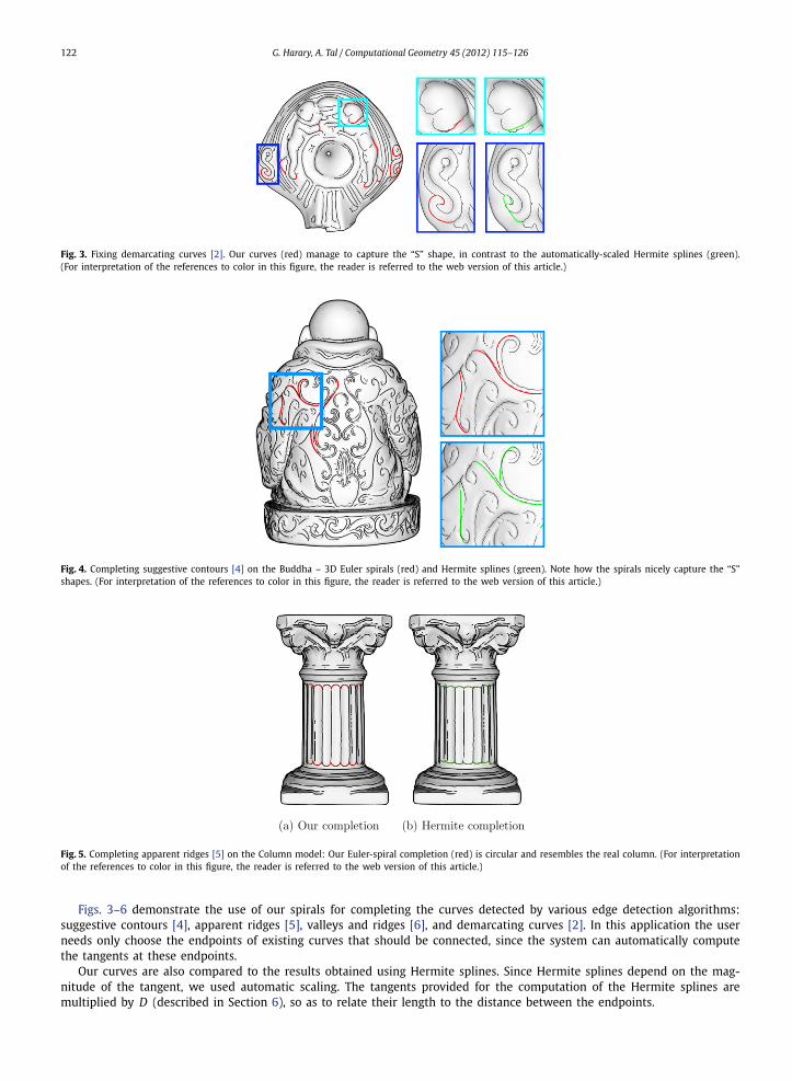
Fig. 4. Completing suggestive contours [4] on the Buddha – 3D Euler spirals (red) and Hermite splines (green). Note how the spirals nicely capture the “S”shapes. (For interpretation of the references to color in this figure, the reader is referred to the web version of this article.)

Fig. 5. Completing apparent ridges [5] on the Column model: Our Euler-spiral completion (red) is circular and resembles the real column. (For interpretationof the references to color in this figure, the reader is referred to the web version of this article.)

Figs. 3–6 demonstrate the use of our spirals for completing the curves detected by various edge detection algorithms:suggestive contours [4], apparent ridges [5], valleys and ridges [6], and demarcating curves [2]. In this application the userneeds only choose the endpoints of existing curves that should be connected, since the system can automatically computethe tangents at these endpoints.

Our curves are also compared to the results obtained using Hermite splines. Since Hermite splines depend on the mag-nitude of the tangent, we used automatic scaling. The tangents provided for the computation of the Hermite splines aremultiplied by D (described in Section 6), so as to relate their length to the distance between the endpoints.

G. Harary, A. Tal / Computational Geometry 45 (2012) 115–126 123

Fig. 6. (a) Completing suggestive contours [4] on the Rocker-arm model. This example illustrates the roundness property of our curve. (b) Completingapparent ridges [5] on the Bust model ((c) – zoom in).

Fig. 7. Analysis of the projected curves of the “S”-shape from Fig. 3. Top: the curvature and the torsion of the 3D curves. Bottom: the curvature and thetorsion of the projected curves. Our projected curve maintain approximately the same properties of the curvature and the torsion, whereas these propertieschange considerably in the case of Hermite spline.

It can be seen that our curves manage to satisfactorily complete the curves, regardless of how they were created. Thetwo features that are most visible in our spirals, are the ability to create perfect circular arcs (Figs. 5, 6) and the “natural”S-shapes (Fig. 4).

In this application, the generated curves should lie on the surface. Since our curves are not constrained to lie on anysurface, the produced 3D Euler curves are projected to the surface. This is done by projecting each point on the curve to itsclosest point onto the mesh. Though this method is straightforward, it yields good results.

To further examine the quality of the projected curves, we compare the curvature and the torsion of the projectedcurves with those of the 3D curves. Fig. 7 shows the results on the “S”-shape completion from Fig. 3. It can be seen thatthe curvature and the torsion of our projected curve are approximately linear. On the other hand, when projecting the 3DHermite spline to the object, the curvature and the torsion change considerably. This is so since our spirals are close to thesurface to start with.

124 G. Harary, A. Tal / Computational Geometry 45 (2012) 115–126

Fig. 8. Completing a broken oil lamp. (a) Archaeological drawing of a lamp [42]. (b–c) Completion of a similar lamp in 3D. The 3D Euler spirals (red)are more appealing than the Hermite splines (green) due to the nice circles produces. This is guaranteed by the roundness property of our curves. (Forinterpretation of the references to color in this figure, the reader is referred to the web version of this article.)

Fig. 9. Completing ridges [6] on a broken amphora.

7.2. Shape illustration in archaeology

Archaeology has recently attracted a lot of attention in geometry processing [43–46]. In this paper we focus on oneaspect of archaeological research – relic completion. Many of the artifacts found by the archaeologists are scanned and needto be processed and analyzed. These artifacts are often broken and eroded and thus are difficult to handle. One specificproblem is the drawing of the artifact, which is traditionally performed manually by archaeological artists in 2D, as shownin Fig. 8(a). This is an expensive and time-consuming procedure, which is prone to biases and inaccuracies. Our curvespropose a 3D alternative, as illustrated in Fig. 8(b–c).

Figs. 9–12 show several additional models, which show that our completed curves are not only more appealing, but alsobetter resemble the shape of the original unbroken models. For example, the curl completion in Fig. 10 demonstrates theS-shape property of our spirals, while the ear completion illustrates a more “circular” shape. Fig. 11 demonstrates that sinceour curves have more “volume”, they avoid intersecting the mesh, which might occur when using the Hermite completion.

Fig. 12 shows a comparison also to the 3D Biarcs of [24]. In addition to a visual comparison, we also depict the curves’curvature and torsion. It can be seen that at the point of connection between the planar arcs, Biarcs have a singular torsionpoint and a large jump in the curvature.

7.3. Running times

The algorithm was implemented in Matlab and C and ran on a 2 Ghz Intel Core 2 Duo-processor laptop with 2 Gb ofmemory. The running time, which depends on the complexity of the required interpolation curve, is 0.01–0.5 second for thecurves demonstrated in this paper. The further the curve is from being planar, the longer the time required. This is probablydue to initializing the torsion to zero. The size of the model has little affect on the time; it is relevant only when projectionis performed. The projection itself is straightforward and quick to compute.

8. Conclusion

This paper presents a novel definition of curves, which extends the 2D Euler spiral to 3D. We proved that for givenparameters, a unique curve always exists. Moreover, we showed that our curves satisfy several desired aesthetic proper-ties, including invariance to similarity transformation, symmetry, extensibility, smoothness, and roundness. Given boundary

G. Harary, A. Tal / Computational Geometry 45 (2012) 115–126 125

Fig. 10. Completing a (manually) broken head sculpture. The 3D Euler spirals (red) nicely compute the S-shaped curl. The Euler completion of both the curland the ear are more similar to the original model than the Hermite completion (green). (For interpretation of the references to color in this figure, thereader is referred to the web version of this article.)

Fig. 11. Completion of a broken Hellenistic lamp. Ridges and valleys [6] are used to determine initial conditions. Our curves (red) manage to capture thetrue volume of the shape, while the Hermite splines (green) intersect the broken model. (For interpretation of the references to color in this figure, thereader is referred to the web version of this article.)

Fig. 12. The completion of a (manually) broken pot. (a–d) Our curves better resemble the original unbroken model. (e–f) The curvature and the torsion ofthe right curve. Biarcs have a singular torsion point and a large jump in the curvature.

conditions – endpoints and tangents – this paper proposed a novel technique for generating these curves, based on thegradient-descent approach.

The utility of our curves is demonstrated for edge completion on polyhedral surfaces and for artifact illustration inarchaeology – a task that is traditionally performed manually in 2D. In archaeology, when automatic 3D curve drawingreplaces the traditional manual 2D drawing, automatic or interactive curve completion, would be the only alternative. We

126 G. Harary, A. Tal / Computational Geometry 45 (2012) 115–126

believe that the proposed curves may be found a feasible alternative for additional applications involving shape design,artistic design, and shape analysis.

In the future, we wish to prove existence of the curves given point–tangent boundary conditions. In 2D, an algorithmwas first established [16] before existence was proved several years later [36]. We hope that the same will happen in 3D.In practice a solution exists for all the inputs we tried.

Acknowledgements

This research was supported in part by the Israel Science Foundation (ISF) 628/08, the Goldbers Fund for ElectronicsResearch, and the Ollendorff foundation. We thank Dr. A. Gilboa and the Zinman Institute of Archaeology at the Universityof Haifa for providing the archaeological models. The other models are courtesy of the AIM@SHAPE Shape Repository andthe MIT CSAIL database.

References

[1] G. Harary, A. Tal, The natural 3D spiral, Computer Graphics Forum 30 (2) (2011) 237–246.[2] M. Kolomenkin, I. Shimshoni, A. Tal, Demarcating curves for shape illustration, ACM Transactions on Graphics 27 (5) (2008) 157, 1–9.[3] R. Zatzarinni, A. Tal, A. Shamir, Relief analysis and extraction, ACM Transactions on Graphics 28 (5) (2009) 136, 1–9.[4] D. DeCarlo, A. Finkelstein, S. Rusinkiewicz, A. Santella, Suggestive contours for conveying shape, ACM Transactions on Graphics 22 (3) (2003) 848–855.[5] T. Judd, F. Durand, E. Adelson, Apparent ridges for line drawing, ACM Transactions on Graphics 26 (3) (2007) 19, 1–7.[6] S. Yoshizawa, A. Belyaev, H.P. Seidel, Fast and robust detection of crest lines on meshes, in: ACM Symposium on Solid and Physical Modeling, 2005,

pp. 227–232.[7] G. Barequet, S. Kumar, Repairing CAD models, in: IEEE Visualization, 1997, pp. 363–370.[8] G. Barequet, M. Sharir, Filling gaps in the boundary of a polyhedron, Computer Aided Geometric Design 12 (2) (1995) 207–229.[9] A. Sharf, M. Alexa, D. Cohen-Or, Context-based surface completion, ACM Transactions on Graphics 23 (3) (2004) 878–887.

[10] C. De Boor, A Practical Guide to Splines, Springer, 2001.[11] G. Farin, Curves and Surfaces for Computer Aided Geometric Design, Academic Press, 1993.[12] R. Farouki, C. Neff, Hermite interpolation by Pythagorean hodograph quintics, Mathematics of Computation 64 (212) (1995) 1589–1609.[13] R. Farouki, Pythagorean-Hodograph Curves: Algebra and Geometry Inseparable, Springer, 2008.[14] M. Singh, J. Fulvio, Visual extrapolation of contour geometry, PNAS 102 (3) (2005) 939–944.[15] H. Moreton, C. Séquin, Functional optimization for fair surface design, ACM SIGGRAPH 26 (2) (1992) 167–176.[16] B. Kimia, I. Frankel, A. Popescu, Euler spiral for shape completion, International Journal of Computer Vision 54 (1) (2003) 159–182.[17] R. Levien, The Euler spiral: a mathematical history, Tech. Rep. UCB/EECS-2008-111, EECS Department, University of California, Berkeley, 2008.[18] J. McCrae, K. Singh, Sketching piecewise clothoid curves, Computers & Graphics 33 (4) (2009) 452–461.[19] D. Knuth, Mathematical typography, Bulletin AMS 1 (2) (1979) 337–372.[20] G. Harary, A. Tal, 3D Euler spirals for 3D curve completion, in: Annual Symposium on Computational Geometry, 2010, pp. 393–402.[21] G. Harary, A. Tal, Visualizing 3D Euler spirals, in: Annual Symposium on Computational Geometry, 2010, pp. 107–108, http://www.computational-

geometry.org/SoCG-videos/socg10video/.[22] S. Ullman, Filling-in the gaps: The shape of subjective contours and a model for their generation, Biological Cybernetics 25 (1) (1976) 1–6.[23] M. Brady, W. Grimson, D. Langridge, Shape encoding and subjective contours, in: First Annual National Conference on Artificial Intelligence, 1980,

pp. 15–17.[24] K. Chui, W. Chiu, K. Yu Direct, 5-axis tool-path generation from point cloud input using 3D biarc fitting, Robotics and Computer-Integrated Manufac-

turing 24 (2) (2008) 270–286.[25] T. Sharrock, R. Martin, Biarc in three dimensions, in: The Mathematics of Surfaces II, 1996, pp. 395–411.[26] W. Rutkowski, Shape completion, Computer Graphics and Image Processing 9 (1979) 89–101.[27] B. Horn, The curve of least energy, ACM Transactions on Mathematical Software 9 (4) (1983) 441–460.[28] R. Levien, The Elastica: a mathematical history, Tech. Rep. UCB/EECS-2008-103, EECS Department, University of California, Berkeley, 2008.[29] E. Mehlum, Appell and the apple (nonlinear splines in space), in: Mathematical Methods for Curves and Surfaces, 1995, pp. 365–384.[30] D. Mumford, Elastica and computer vision, Algebraic Geometry and Its Applications (1994) 491–506.[31] M. Born, Untersuchungen über die Stabilität der elastischen Linie in Ebene und Raum: Unter verschiedenen Grenzbedingungen, Dieterich, 1906.[32] G. Glaeser, H. Stachel, Open Geometry: OpenGL+ Advanced Geometry, Springer, 1999.[33] E. Mehlum, Nonlinear splines, Computer Aided Geometric Design (1974) 173–207.[34] D. Meek, D. Walton, Clothoid spline transition spirals, Mathematics of Computation 59 (199) (1992) 117–133.[35] D. Walton, D. Meek, A controlled clothoid spline, Computers & Graphics 29 (3) (2005) 353–363.[36] D. Walton, D. Meek, G1 interpolation with a single Cornu spiral segment, Journal of Computational and Applied Mathematics 223 (1) (2007) 86–96.[37] L. Guiqing, L. Xianmin, L. Hua, 3D discrete clothoid splines, in: International Conference on Computer Graphics, 2001, pp. 321–324.[38] M. do Carmo, Differential Geometry of Curves and Surfaces, Prentice Hall, 1976.[39] A. Forsyth, Calculus of Variations, Dover, NY, 1960.[40] W. Graustein, Differential Geometry, Dover, 2006.[41] U. Ascher, L. Petzold, Computer Methods for Ordinary Differential Equations and Differential-Algebraic Equations, Society for Industrial Mathematics,

1998.[42] E. Stern, Excavations at Dor, Institute of Archaeology of the Hebrew University, Jerusalem, 1995.[43] B. Brown, C. Toler-Franklin, D. Nehab, M. Burns, D. Dobkin, A. Vlachopoulos, C. Doumas, S. Rusinkiewicz, T. Weyrich, A system for high-volume acqui-

sition and matching of fresco fragments: reassembling Theran wall paintings, ACM Transactions on Graphics 27 (3) (2008) 84, 1–10.[44] D. Koller, J. Trimble, T. Najbjerg, N. Gelfand, M. Levoy, Fragments of the city: Stanford’s digital forma urbis romae project, Journal of Roman Archaeol-

ogy 61 (2006) 237–252.[45] H. Rushmeier, Egypt eternal experiences and research directions, Recording, Modeling and Visualization of Cultural Heritage (2006) 22–27.[46] A. Vrubel, O. Bellon, L. Silva, A 3D reconstruction pipeline for digital preservation, Computer Vision and Pattern Recognition (2009) 2687–2694.