Inverse Problems 16 (2000) 1297-1322. Printed in the UK PH: S0266-5611(00) 14585-X

3D electromagnetic inversion based on quasi-analytical approximation

Michael Zhdanovt and Gabor Hursan University of Utah, Department of Geology and Geophysics, Salt Lake City, UT 84112, USA

Received 3 March 2000

Abstract. In this paper we address one of the most challenging problems of electromagnetic (EM) geophysical methods: three-dimensional (3D) inversion of EM data over inhomogeneous geological formations. The difficulties in the solution of this problem are two-fold. On the one hand. 3D EM forward modelling is an extremely complicated and time-consuming mathematical problem itself. On the other hand, the inversion is an unstable and ambiguous problem. To overcome these difficulties we suggest using, for forward modelling, the new quasi-analytical (QA) approximation developed recently by Zhdanov et al (Zhdanov M S, Dmitriev V I, Fang Sand Hursan G 1999 Geophvsics at press). It is based on ideas similar to those developed by Habashy et al (Habashy T M, Groom R Wand Spies B R 1993 J. Geophvs. Res. 98 1759-75) for a localized nonlinear approximation, and by Zhdanov and Fang (Zhdanov M S and Fang S 1996a Geophysics 61646-65) for a quasi-linear approximation. We assume that the anomalous electrical field within an inhomogeneous domain is linearly proportional to the background (normal) field through a scalar electrical reflectivity coefficient. which is a function of the background geoelectrical cross-section and the background EM field only. This approach leads to construction of the QA expressions for an anomalous EM field and for the Frechet derivative operator of a forward problem. which simplifies dramatically the forward modelling and inversion. To obtain a stable solution of a 3D inverse problem we apply the regularization method based on using a focusing stabilizing functional introduced by Portniaguine and Zhdanov (Portniaguine 0 and Zhdanov M S 1999 Geophvsics 64 874-87). This stabilizer helps generate a sharp and focused image of anomalous conductivity distribution. The inversion is based on the re-weighted regularized conjugate gradient method.

1. Introduction

Electromagnetic (EM) geophysical methods are widely used in the study of the internal structure of the earth in mineral, oil and gas prospecting, tectonic studies, and environmental assessment and monitoring. They provide unique information about the geological structures, petrophysical properties, lithologic characteristics, and thermodynamic and phase status of the rocks in the Earth's interior. The future perspective in EM geophysical methods lies in the development of multi-transmitter and multi-receiver methods with an array observation system analogous to a seismic data acquisition system. Therefore, the main efforts in the development of an interpretation technique has to be concentrated on creating three-dimensional (3D) methods of analysis of the array EM data. At the same time, the development of effective interpretation schemes for 3D inhomogeneous geological structures is still one of the most challenging problems in geophysics.

During the last decade, considerable advances have been made in forward modelling, especially in 3D cases (Madden and Mackie 1989, Wannamaker 1991, Xiong 1992, Newman

t To whom correspondence should be addressed.

0266-5611/00/051297+26$30.00 © 2000 lOP Publishing Ltd 1297

1298 M Zhdanov and G Hursan

and Alumbaugh 1997, Avdeev et a11998, Druskin et aI1999). Also, we can observe remarkable progress in the development of a multi-dimensional interpretation technique. Several papers have been published during the last few years on 3D inversion of EM data (Eaton 1989, Madden and Mackie 1989, Smith and Booker 1991, Lee and Xie 1993, Oristaglio et al 1993, Pellerin et al 1993, Nekut 1994, Torres-Verdin and Habashy 1994, Zhdanov and Keller 1994, Xie and Lee 1995, Newman and Alumbaugh 1997, Zhdanov and Fang 1996b, 1999 and Alumbaugh and Newman 1997). Note that this reference list includes the papers which focus on inversion in the Earth and are most relevant to our paper only.

The methods for solving multi-dimensional EM inverse problems are usually based on the optimization of the model parameters by applying different inversion schemes. The key problems in the optimization technique is the calculation of the Frechet derivative (sensitivity matrix), which usually requires a lot of computational time.

Thus, speaking about the future perspective on developments in EM research, we should emphasize that the main goa] will be multi-dimensional modelling and inversion, oriented to the use of the array EM data. In this connection one of the key problems is the speed of multi­dimensional modelling codes. A powerful tool for EM numerical modelling and inversion is the integral equation method (Hohmann 1975, Weidelt 1975, Dmitriev and Pozdnyakova 1992). This method is based on the reduction of the EM problem to a system of integral equations with respect to the excess current i' within the inhomogeneity. The main difficulty of this technique is related to the large size of the matrix of the linear system of equations, which could require a great deal of computer memory and time for calculations.

Another way to overcome this problem is to use the Born-type approximations for fast forward modelling (Born 1933, Habashy et al 1993, Torres-Verdin and Habashy 1994). These approximate, but accurate enough, forward solutions provide a linear forward modelling operator which can be used for the rapid inversion of the multi-dimensional data (Berdichevsky and Zhdanov 1984, Habashy et al 1986, Oristaglio 1989). Habashy et al (1993) developed a generalized Born approximation (so-called localized nonlinear (LN) approximation), which improved significantly the accuracy of the approximate solutions, and applied it to inversion (Torres-Verdin and Habashy 1994). In our recent publications, (Zhdanov and Fang 1996a, b, 1997, 1999), we modified this approach to 3D EM modelling and inversion, introducing a quasi-linear (QL) approximation. Within the framework of this method, the anomalous electrical field inside an inhomogeneous domain is linearly proportional to the background (normal) field through an electrical reflectivity tensor ~, which is a function of the background geoelectrical cross-section and the background EM field only. The electrical reflectivity tensor ~ can be determined by an approximate analytical solution of the corresponding integral equation (Zhdanov et al 1999). This approach leads to a construction of the quasi­analytical (QA) expressions for an anomalous EM field and the Frechet derivative operator of a forward problem, which simplifies dramatically the forward EM modelling and inversion for inhomogeneous geoelectrical structures.

Another critical problem in inversion of EM data is developing a stable inverse problem solution which can produce, at the same time, a sharp and focused image of the target. The traditional inversion methods are usually based on the Tikhonov regularization theory, which provides a stable solution of the inverse problem. This goal is reached, as a rule, by introducing a maximum smoothness stabilizing functional. The obtained solution provides a smooth image, which in many practical situations does not describe the examined object properly.

Recently, a new approach to reconstruction of noisy images has been developed in a number of papers (Rudin et al 1992, Vogel and Oman 1998). It is based on a total variational stabilizing functional which requires that the model parameter distribution be of bounded variation. This requirement is much weaker than one of maximum smoothness because it can

1299 Quasi-analvtical inve rsion

be applied even to discontinuous functions. In this way the total variation method produces better quality images for blocky structures. However, it still decreases the boundaries of the model parameter variation and therefore distorts the real image.

We consider different ways of focusing EM images using specially selected stabilizing functionals. In particular. we use a new stabilizing functional which minimizes the area where strong model parameter variations and discontinuity occur. This functional was originally introduced for the solution of a gravity inverse problem (Portniaguine and Zhdanov 1999). We call this new functional a focusing stabilizer. We demonstrate how the focusing stabilizer helps to generate a stable solution of the EM inverse problem for complex objects and helps to generate much more 'focused' EM images than conventional methods.

Thus, the main goal of this paper is to demonstrate that a relatively simple QA expression for EM response over arbitrary 3D inhomogeneous structures, derived by Zhdanov et al (1999), in combination with the focusing stabilizer, can be used for developing a new generation of fast 3D EM inversion techniques.

2. QA solutions for a 3D EM field

For completeness. we begin our paper with the formulation of the basic principles of QL and QA approximations. Consider a 3D geoelectrical model with a background (normal) complex conductivity o-/J and local inhomogeneity D with the arbitrary spatial variations of complex conductivity 0- = CJh + ~O-. We assume that u. = lJ-o = 4JT X 10-7 H m -I, where flo is the free-space magnetic permeability. The model is excited by an EM field generated by an arbitrary source. This field is time harmonic as e- icvl . Complex conductivity includes the effect of displacement currents: 0- = (J - i(vs, where (J and E are electrical conductivity and dielectric permittivity, respectively. The EM fields in this model can be presented as a sum of background (normal) and anomalous fields:

H IJE = E h + Ell. H = + H", (I)

where the background field is a field generated by the given sources in the model with the background distribution of conductivity o-b, and the anomalous field is produced by the anomalous conductivity distribution ~O-.

It is well known that the anomalous field can be presented as an integral over the excess currents in inhomogeneous domain D (Hohmann 1975, Weidelt 1975):

ElI(rj) = ( Ch;(rj I r)jll(r) dv = GE(/I), (2)Jf) Hll(rj) = Iv c,,« I r)j{/(r)dv = Gf/(jll), (3)

where CE (rj I r) and Cf/ (rj I r) are the electric and magnetic Green tensors defined for an unbounded conductive medium with the background conductivity o-b; G E and G Hare corresponding Green linear operators, and the excess current j{/ is determined by the equation

i" = ~o- E =~o-(Eb + Ell). (4)

Using Green operators, one can calculate the EM field at any point rj, if the electric field is known within the inhomogeneity.

E(rj) = GfJ~o-E) +Eh(rj), (5)

H(rj) = Gf/(~CJE) + Hh(Tj). (6)

Expression (5) becomes the integral equation with respect to electric field E(r), if rj E D.

1300 M Zhdanov and G Hursan

The QL approximation is based on the assumption that the anomalous field E(/ inside the inhomogeneous domain is linearly proportional to the background field E IJ through some tensor ~ (Zhdanov and Fang 1996a):

E(/(r) ~ ~Cr)Eh(r). (7)

Note that, in the framework of the QL approach, the electrical reflectivity tensor can be selected to be a scalar one (Zhdanov and Fang 1996a):

A = XI. (8)

where i is a unit tensor. This assumption, of course, reduces the areas of practical applications of the QA approximations because, in this case, the anomalous (scattered) field is polarized in a

direction parallel to the background field within the inhomogeneity. However, in a general case the anomalous field can be polarized in a different direction from the background field, which could generate additional errors in the scalar QA approximation. Therefore, this particular choice may be a cause of difficulties in the case of elongated bodies (e.g. needle-like) or of flat bodies (e.g. plate-like), while strong conductivity contrast could also be a source of errors, as well as fast variations of the background field in the body volume. Nevertheless, numerical modelling demonstrates that the corresponding errors are within a few percentages

if observations are conducted in the far zone of the transmitter, or in the case of plane-wave excitation (Zhdanov et al 1999).

Substituting formulae (7) and (8) into (5), we obtain the QL approximation E QL(r) for

the anomalous field:

h).EQL(rj) = Gd~o-(l +A.(r))E (9)

The last formula can be used to derive a QL equation with respect to the electrical reflectivity coefficient X:

hA(r, )E (rj) = G Id~o-A(r )Eh] + E B(rj), (10)

where E B (rj) is the Born approximation

EB(rj) = GF:(~o-Eh) = ( GE(rj I r)~o-(r)Eh(r)dv, (11)Jf) and Gd~o-A(r)Eh] linearly depends on A(r):

G rJ~ 0- A(r )E h] = { G t: (r j I r) L'l(J ( r )X(r )E IJ ( r) dv . ( 12) Jf)

Following Habashy et a! (1993) and Torres-Verdin and Habashy (1994), we can take into

account that the Green tensor Gr. v: I r) exhibits either singularity or a peak at the point where rj = r. Therefore, one can expect that the dominant contribution to the integral G ElL'lo- AEh]

in equation (10) is from some vicinity of the point rj = r. Assuming also that A(rj) is a slowly varying function within domain D, one can write

A(rj)Eh(rj) ~ A(rj)Gd~o-Eh]+EB(rj) = A(rj)EB(rj) + EB(rj}. (13 )

Taking into account that we are looking for a scalar reflectivity tensor, it is useful to introduce a scalar equation on the basis of the vector equation (13). We can obtain a scalar equation by calculating the dot product of both sides of equation (13) and the background electric field:

A(rj )E I) ( rj) . E h*(T'j) = A(rj )E B ( r, ) . E h*(Ti ) + E B ( rj) . E h*(rj ) . ( 14)

where ,*' means complex conjugate vector.

Quasi-analytical inversion 130]

Dividing equation (14) by the square of the background field and assuming that

Eb(rj) . Eb*(rj) i= 0, (15)

we obtain

A(rj) = (16)

where

K(r j) = E H ( rj) . E b*(rj ) Eb (r .) . Eb* (r .) .

.J .J

(17)

Substituting (16) into (9), we finally determine

(J b EQA(rj)=E(rj)-E (rj)

[ A ~o- (r) b = iD GE(rj Ir)l_g(r)E (r)dv. ( 18)

A similar formula can be obtained for the magnetic field:

(J b /, A ~o- (r) bH QA(r /.) = H (r j) - H (r j) = G H (r j I r) E (r) dv . (19)

. . . D . I - g(r)

Formulae (18) and (19) give QA solutions for 3D EM fields. Note that the only difference between the new QA approximation and the Born approximation (I I) is in the presence of the scalar function [I - g(r)r This is why the computational expenses to generate the QA '. approximation and the Born approximation are practically the same. On the other hand, it is demonstrated in Zhdanov et al (1999) that the accuracy of the QA approximation is much higher than the accuracy of the Born approximation.

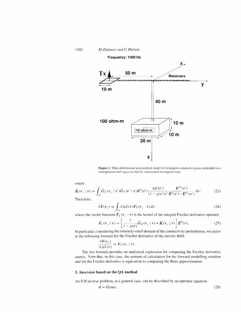
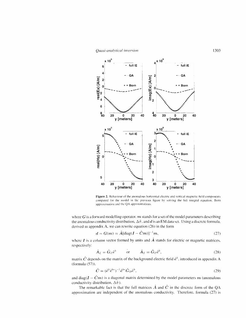
To illustrate this fact we present the results of numerical experiments for the model shown in figure I. It consists of a conductive rectangular prism embedded in a homogeneous half­space excited by a horizontal rectangular loop. The frequency is 1000 Hz and the conductivity ratio between the conductive prism and the homogeneous background is ]O. The receivers are located above the body along the y-axis. Figure 2 shows the real and imaginary parts of the horizontal electric and vertical magnetic components of the scattered field computed by solving the full integral equation (SYSEM code by Xiong (1992» and the approximate solutions. The deviations of the QA approximation from the true solution are invisible, while the Born approximation fails.

Another advantage of using expressions (18) and (19) for forward modelling is the ability to generate a simple formula for the Frechet derivative operator which can be used in inversion algorithms. For example, by introducing a perturbation of the anomalous conductivity 8~o- (r)

we can calculate the corresponding perturbation of the electric field 8E(rj) on the basis of equation (18):

AA 8~0-(r) b /, ~0-(r)8g(r) b 8E(rj) = Gdrj I r) E (r) dv + GE(rj I r) E (r) dv, (20)'1

/,. [) I-g(r) [)' (I-g(r»

where

A8E B(r)· Eh*(r) /, I _ I Eb(r'). Eb*(r) .' 8g(r) = = Gt·(r I r )8~cr(r ) d» . (2] )

Eb(r) . Eb*(r) D . Eb(r) . Eb*(r)

Substituting equation (21) into the second integral in (20) and changing the notations for the integration variables, r ~ r ' and r' -+ r , we obtain

A A~0-(r)8g(r) /,G t: ( r /' I r) 2 E b(r) d v = 8~ 0- (r )K (r /' I r) E h(r) dv . (22)

/,D . (I - g(r» D .

1302 M Zhdanov and G Hursan

Frequency: 1000 Hz

x

-.. SOm Receivers-

.................................... .... ....

y 10 m

40 m

100ohm-m 110 m 110 ohm-cii]

-~~W1om ---~----+-------

20m

z

Figure 1. Three-dimensional geoelectrical model of rectangular conductive prism embedded in a homogeneous hal f-space excited by a horizontal rectangular loop.

where ~a(r') Eb*(r ') I

A I A ( I I ) E b ( ') dv . (23)ic«, I r) = }; Gt(rj I r )GE r r r (I _ g(r'))2 Eh(r')' Eh*(r1) ')

Therefore,

oE(rj) = [ o~a(r)FECrj r) dv, (24)iD I

where the vector function Fe (rj I r) is the kernel of the integral Frechet derivative operator

F£Crj I r) = [__I-ct(rj I r) + K(rj I r)] Eb(r). (25)I - g(r)

In particular, considering the infinitely small domain ofthe conductivity perturbation, we arrive at the following formula for the Frechet derivative of the electric field:

_(}_E_{r_J_) _ Fe (r' I r) a~a(r) - L J •

The last formula provides an analytical expression for computing the Frechet derivative matrix. Note that, in this case, the amount of calculation for the forward modelling solution and for the Frechet derivative is equivalent to computing the Born approximation.

3. Inversion based on the QA method

An EM inverse problem, in a general case, can be described by an operator equation

d = G(m), (26)

Quasi-analytical inversion

9 X 10~~-~-~-l

:1 - lull IE ! QA I

E 2~ I _.

1<c ' 1

1 ~ 0 + + Bo:__ ..

~2 t ------.­Q) ,++ + :to.. 4 I +++ ++++ 1

I ++ ++ 6 I

r 8 L 40

X 10r.-:-----~~~

5............+++ - full IE 1 I +++ I

I

E ~ ~---N Of

I

J: I

::=" i

~ II:

5 L

++++ ++++ j++ ++ , ~~~~ J

20 0 20 40 Y [meters]

9

\+ - QA I

]303

8 X 10l-~--~--hilllEl

I I

......, _. QA j21E,l <c........ _>< .

I + + Born

IIi I

W 0t,--- --_ ... j"'-""" '.... ,­0) + ...----... ++t

++ + I 113 ++ ++ iI

E l + ++ I .- 2 ++ + j I I~ ~ I I+++ +++ I I+++ ,..+++

4 ~I-~__~ __~~ 40 20 0 20 40

Y [meters]

8 X 10 .

'-r--~-

3~++ - full IE

2l ++++

E I \ _. QA 1

<c 1L___ ++ I.... - + + + Born N 0[1 .. - <,~:+ Born....... ,

+ ..... ~ + ..... ++ ........_-­ 0) + --- ­

113 1 +

+++

J .5 2 1 . \ ... +++ ..1

3 I

~~ ~ ~~j__~ ~ ~ ~

40 20 0 20 40 40 20 0 20 40 Y [meters] Y [meters]

Figure 2. Behaviour of the anomalous horizontal electric and vertical magnetic tield components computed for the model in the previous figure by solving the full integral equation, Born approximation and the QA approximations.

where G is a forward modelling operator, m stands for a set of the model parameters describing the anomalous conductivity distribution, ~o-, and d is an EM data set. Using a discrete formula, derived in appendix A, we can rewrite equation (26) in the form

d = G(m) = A[diag(l- Cm.)r1m, (27)

where I is a column vector formed by units and A stands for electric or magnetic matrices, respectively:

~ A I ~ A IA E= GEe) or A E = GEe), (28)

matrix C depends on the matrix of the background electric field e"; introduced in appendix A (formula (57»,

hC = (e h eh* ) - 1eh*GD e , (29)

and diag(l - C'm) is a diagonal matrix determined by the model parameters m (anomalous conductivity distribution, ~a).

The re~larkable fact is that the full matrices A and C in the discrete form of the QA approximation are independent of the anomalous conductivity. Therefore, formula (27) is

1304 M Zhdanov and G Hunan

very efficient in iterative inversion because these matrices have to be precomputed only once for the entire inverse process. Note that the Green functions are computed using the Fast Hankel Transform (Xiong 1992). The only term depending on the model parameters m. is the diagonal matrix diag(I - Cm), which is easy to compute for a given C. These results make QA approximation a very powerful tool in inversion.

Inverse problem (26) is usually ill-posed, i.e. the solution can be non-unique and unstable. The conventional way of solving ill-posed inverse problems, according to regularization theory (Tikhonov and Arsenin ]977, Zhdanov 1993), is based on minimization of the Tikhonov parametric functional:

P" (m) = <p(m) + O's(m), (30)

where <p(m) is a misfit functional between the theoretical values G(m) and the observed data d, s(m) is a stabilizing functional and 0' is a regularization parameter. The optimal value of 0'

is determined from the misfit condition

<p(m) = Oel, (31)

where Oel is the noise level of the data. The minimization problem (30) can be solved using any gradient type technique, say, by the

conjugate gradient (CG) method. The critical point of an inversion algorithm is the calculation of the Frechet derivative (sensitivity) operator F at every iteration of the CG method. The QA solutions described above provide a very effective and elegant way to compute directly the Frechet derivative (sensitivity matrix), outlined in appendix A:

Sd = F(rn)om.

where

F(m) = A{B(m) + diag(m)B2(m)C} (32)

B(m) = [diag(I ­ Cm)r 1 (33)

and diag(m) denotes a diagonal matrix formed by the elements of the vector m. Note again that numerical computations based on formula (32) are very fast and efficient

because the full matrices A and C are precomputed for the background model and are fixed; we update only the diagonal matrix B(m) on each iteration of the inverse process.

4. Principles of imaging geological structures with sharp geoelectrical boundaries

According to the basic principles of the regularization method, we have to find the model m a ,

a quasi-solution of the inverse problem (26), that minimizes the parametric functional (30)

P" (m) = min. (34)

Usually, the misfit functional is specified as

¢(m) = IIWd(G(m) - d)11 2 = (G(m) - d)*Wj(G(m) - d), (35)

where Wd is some weighting matrix of data and symbol '*' means transposed complex conjugated matrix.

There are several common choices for stabilizers in the parametric functional (30). One is based on the least squares criterion. Another stabilizer uses a minimum norm of difference between the selected model and some a priori model. For example, the stabilizer may be selected to be equal to

~ 2 ~ ~

sCm) = IIWI/l(m - m apr) II = (m - mapr)*lV;~(m - m apr). (36)

1305 Quasi-analytical inversion

where Wm is some weighting matrix of model parameters and rnapr is some a priori reference model, selected on the basis of all available geological and geophysical information about the area under investigation. The solution of the minimization problem (34) with the misfit and stabilizing functionals, determined by equations (35) and (36), can be obtained by the regularized conjugate gradient (RCG) method (see appendix B).

The stabilizer (36) applied to the gradient of the model parameters brings us to a maximum smoothness stabilizing functional. It has been successfully used in many inversion schemes developed for EM data interpretation (Berdichevsky and Zhdanov 1984, Constable et al 1987, Smith and Booker 1991, Zhdanov and Fang 1996b). This stabilizer produces smooth models, which in many practical situations does not describe properly the real blocky geological

structures. In Portniaguine and Zhdanov (1999), another stabilizing functional was considered which

minimized the area of the anomalous conductivity distribution. This functional was called a minimum support (MS) functional.

The MS functional can be described as follows. Consider the following integral of the model parameter distribution:

2

J/3(m) = 1-2--') m

dv. (37) v m +£­

We introduce the support of m (denoted sptm) as the combined closed subdomains of V where m #- O. We call sptm a model parameter support. Then expression (37) can be modified:

1 Jf;(m) = {, [1 -~] dv = sptm - £2 ( -2- dv. (38)- '1

}sPlm m + 8 }SPlm m + 8"­

From the last expression we can see that

Jf;(m) -+ sptm. if 8 -+ O. (39)

Thus, integral J, (m) can be treated as a functional, proportional (for a small 8 ) to the model parameter support. We can use this integral to introduce a MS stabilizing functional SMS (m)

as follows:

1 (m ­ mapr)2 SMS(m) = Lim - mapr) = 2 - dv. (40)

v (m - m apr) + 8

It is proved in Portniaguine and Zhdanov (1999) that the MS functional satisfies the Tikhonov criterion for a stabilizer. For discrete model parameters rn, functional SMS can be written using matrix notations

2])-1 (rnsMS(rn) = (rn - rnapr)*(diag[(rn - rnapr) 2 + 8 - rnapr). (41 )

We can introduce a variable diagonal weighting matrix We (rn) according to the formula

~ " 2 2 1/2We(rn) = dlag[(rn - rnapr) + 8] . (42)

Then the stabilizing functional can be written as the weighted least square norm of the model

parameters

SMS(rn) = (rn - rnapr)*We-2(rn - rnapr)' (43)

Note that it is still important to use in the inversion scheme the permanent weights of model parameters Wm introduced in the original stabilizer (36). The fact is that the sensitivity of the data to the different model parameters is different because the contribution of the different parameters in the observation is also different. For example, the effect of the shallow parts of the geoelectrical cross-section is much more significant than the effect of the deep structures.

1306 M Zhdanov and G Hunan

The weighting matrix TV;11 can be constructed in such a way that the sensitivity of the data to the weighted model parameters will become more or less equal. We have demonstrated in Mehanee and Zhdanov (1998) that the matrix TV;n with this property can be determined as the square root of the integrated Frechet derivative (sensitivity) matrix:

TV;/1 Js, (44)

where S is the diagonal matrix formed by the integrated sensitivities of the field data d to the parameter mi ; determined as the ratio

Ilodll PMS, = - = L(Fid-. (45) omk i

In the last formula Fi k are the elements of the Frechet derivative matrix P(mo) for the initial model.

In a similar way, we can define the data-weighting matrix as

W,1 = diag(4j~(Fi[)2). (46)

These weights make normalized data less dependent on the frequency and distance from the anomalous domain, which improves the resolution of the inverse method.

The parametric functional we seek to minimize can be written using matrix notations:

P" (m) = (G(m) - d)*W](G(m) - d) + a(m - mapr)*We-2W;~ (m - m apr ) = min.

(47)

Note that in this case we implement the MS functional by introducing the variable weighting matrix We. Therefore, the problem of the minimization of the parametric functional introduced by equation (47) can be treated in a similar way to the minimization of the conventional Tikhonov functional with the least square stabilizer (36). The only difference is that now we introduce some variable weighting matrix, We' for model parameters. This method is similar to the variable metric method. However, in our case, the variable weighted metric is used in calculation of the stabilizing functional only.

The minimization of the parametric functional (47) can be carried out using the CG method similar to one outlined in appendix B. Numerical calculations, however, demonstrate that the most efficient way to solve this problem is based on minimization in the space of weighted parameters. We will discuss the basic ideas of this method in the next section.

5. Minimization in the space of weighted parameters

The minimization problem (47) can be reformulated using the space of weighted parameters: II' ~ _I A

m W;, vv,/Im. (48)

We introduce also the weighted data

dlJ' = Wi/d. (49)

We can consider the forward operator, which relates the new weighted parameters mil' to the weighted data,

d" = GII'(mlJ') = Wi/G(W;~IW('ml1'). (50)

Note that from formula (50), we obtain a simple relationship between the Frechet derivative matrices of the new, G l1' (rn"), and old, G(m), forward modelling operators:

6GII'(m U ' ) = P .Srn" = W: oGW- 1 W: mil'11 d III (' •

1307 Quasi-analytical inversion

Therefore, _IA A A A A

s; = W dF "";ll We' (51)

Using these notations we can rewrite the parametric functional (47) as follows:

pet( 11') = (,G1I'(m l1' ) _ dW)*(GW(mW ) _ d W) +a(mu: _ m'" )*(, H' _ H') = ' m apr m nun .m apr

(52)

Note that the unknown parameters now are weighted model parameters m 11'. In order to obtain the original conductivity distribution we have to apply inverse weighting to the result of the minimization of the parametric functional (52):

A A_I 11'

m -"";n Wem, . (53)

The numerical experiments show that, as a rule, the iterative process converges faster for (52) than for (47). The minimization method in the space of weighted parameters is similar to the RCG method described in appendix B. One can find a detailed description of the re-weighted RCG method in the space of weighted parameters in appendix C.

6. Model studies

6.1. Model 1

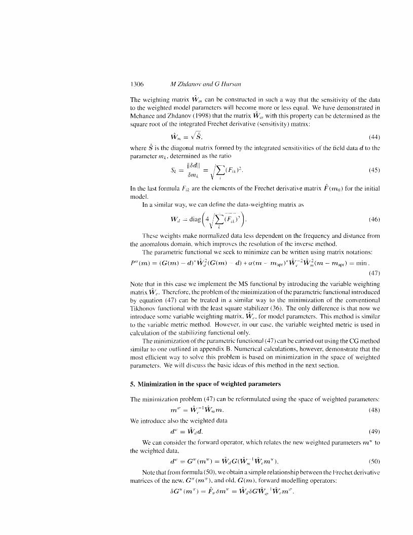
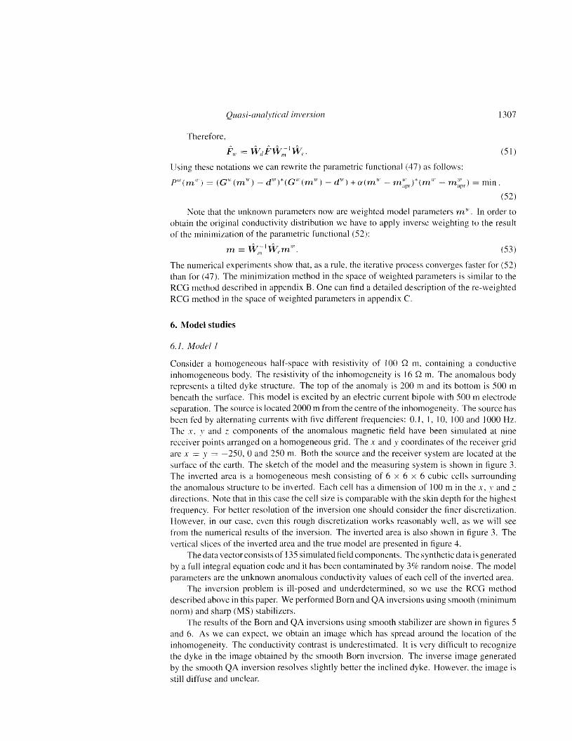
Consider a homogeneous half-space with resistivity of 100 Q m, containing a conductive inhomogeneous body. The resistivity of the inhomogeneity is 16 Q m. The anomalous body represents a tilted dyke structure. The top of the anomaly is 200 m and its bottom is 500 m beneath the surface. This model is excited by an electric current bipole with 500 m electrode separation. The source is located 2000 m from the centre of the inhomogeneity. The source has been fed by alternating currents with five differenr frequencies: 0.1, I, 10, 100 and 1000 Hz. The .r , y and z components of the anomalous magnetic field have been simulated at nine receiver points arranged on a homogeneous grid. The x and y coordinates of the receiver grid are .X- = Y = -250, a and 250 m. Both the source and the receiver system are located at the surface of the earth. The sketch of the model and the measuring system is shown in figure 3. The inverted area is a homogeneous mesh consisting of 6 x 6 x 6 cubic cells surrounding the anomalous structure to be inverted. Each cell has a dimension of 100 m in the x, .\' and z directions. Note that in this case the cell size is comparable with the skin depth for the highest frequency. For better resolution of the inversion one should consider the finer discretization. However, in our case, even this rough discretization works reasonably well, as we will see from the numerical results of the inversion. The inverted area is also shown in figure 3. The vertical slices of the inverted area and the true model are presented in figure 4.

The data vector consists of 135 simulated field components. The synthetic data is generated by a full integral equation code and it has been contaminated by 3% random noise. The model parameters are the unknown anomalous conductivity values of each cell of the inverted area.

The inversion problem is ill-posed and underdetermined, so we use the RCG method described above in this paper. We performed Born and QA inversions using smooth (minimum norm) and sharp (MS) stabilizers.

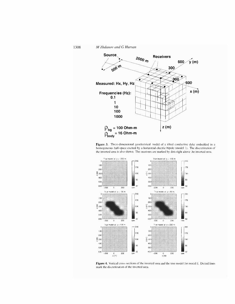
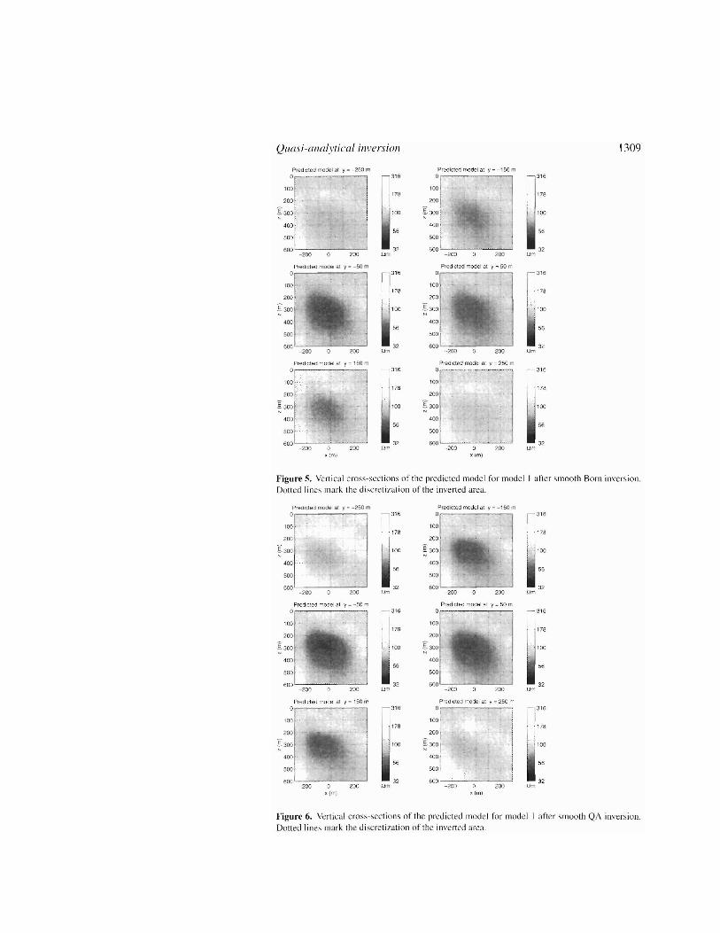
The results of the Born and QA inversions using smooth stabilizer are shown in figures 5 and 6. As we can expect, we obtain an image which has spread around the location of the inhomogeneity. The conductivity contrast is underestimated. It is very difficult to recognize the dyke in the image obtained by the smooth Born inversion. The inverse image generated by the smooth QA inversion resolves slightly better the inclined dyke. However, the image is still diffuse and unclear.

1308 M Z/U/WlOl' and G Hursan

s ~urce'e <000 Receivers

/:~----~ /; . /';,r::,~~------_

Measured: Hx, Hy, Hz I

Frequencies (Hz): 0.1

1 10 100 1000

z (m) Pb9 = 100 Ohm-m () = 16 Ohm-m t1>ody

-I-~:7-----

Fi gure 3. Three-dimensional gcoc lcctrical model of a tilted con ductive dyke embedded in a homogeneous ha lf-space excited by a hor izontal electri c hipol e (model 1). The discreti zation of the inverted area is a lso show n. T he rece ivers are ma rked by dot s right abov e the inverted area .

True model at y::: - 250 m

100 '

200

'[ 300 N

400

500

600 L-1 - - - __-J -200 0 200

True model at y = - SOm ~~

200

Truo model at y::: 150 m

Or 100

200

'[300

400

500

True model at y ::: ~ 1 50 m 316

0 1 100 1.

178 1200

100 ~ 3oo 1 56 400 /

500

32 600 -----­U."

-l 316

I:178

i I 1100

56

32Um 200

316

100 178

200

100 :[ 300

400 56

500

-,- ­- 200 0 200

True model at y :::250 m ~

600 1 I 600 32 ' I -200 0 200 Um - 200 0 200

x Im} x tm)

6°0(m)

316

178

100

56

32 llm

56

32 U rn

Figure 4. Verti cal cross-sections of the inverted area and the true model for model I . Dotted line s mark the discretization of the inverted area.

1309 Quasi -analytical inversion

Predicted mmlel <II 'I :: - 250 m

o! ioo,i 200!

- I

'=1 I600 - - - - - -,.,,,--

Prooictod mode l at y - - 150 m 316 o~. _ ---

100 176

200

100 "[300

400 56

500

32 000 ' !

- 200 200 Urn - ;>00 200 Urn

200

178

reo

56

0r.-y = - 50 mP,e<liCled rnoo et a t

100 · .

200 .

~ ::. :1, :.

- 200 a 200 Um

Precctee mo del at y = 150 m

lo0r:lo · i : . :. j I ::: · : ~. .·1

400 f

500 L-~ 60 0 1 I

' DO

200

~ :[ 300

316

.1 78

1 j 100

56

32

316

178

wo

56

32

3 16

178

100

56

32

316

' 78

100

56

32 - 200 0 200 11fT' a 200 um

xum x {m)

Figure 5. Vertical cross-scctions of the predicted I11od.:1for model I after smo oth Born inversion. Dotted lines mark the disc retization of the inverted area.

Precncreo model at v > -250 m II 316 Or-- ,

I I

~ 30 0 1 _..

i

400

.-:3160 1

100 ; I I I 1178 1178

400 -. .:::. .

56 I f 500 . 500 "':l~ r600 32 600

-200 3 200 U rn - 200 0 200

1100

. 56

Predicted mod el at y = 50 III O. ,..., 3 16

roo1 1178

.s 300 1 I

: 1600

• -

I I I j 178 _ I I 1 ' 00~:!.

~

40° 1 . . 56

500 1 ~:..-.'" fiOD . ------ ---- - - - • 32 600 '

:lJ - 32

- 200 0 200 Um - 200 a 200 <lm

Pred icted model at y = ' 50 m Preorcteo model at y = 250 m 0 , 3W

j Or-

j !,78

- I I; Wr: n

~ 3001 _ . I 1' 00

56 . 56 500; ::~ ! . ..' ..' 600 1 'ti m 1 . 32 600 - 32

- 200 0 200 um -2 00 0 200 nm

100 1 ' i

J

x (m) x (m)

Figure 6. Vertical cross-sec tions of thc predicted model for model I afte r smooth QA inversion . Dotted lines mark the discreti zation of the inverted arca.

1310 M Zhdauov and G Hursan

Predicted mod el at y ==- 250 m Pred icted model <'I I y _ -150 m

il lOoo

°' OOO

101

~ i £ , 300 . .i '.I

1

400

500 . ,

600

316 316 200 J

- !j . 11:L nJ100 5..300 " 1 [ I 100

1 .... 400 1

32 32

:: i10 10 - 200 0 200 Urn - 200 0 200 um

__

Predicted modal A! y == 50 rn

1 ' 1000 -----1 3 16 E-.::''J"":___ 300' 00 ,

32 40000 . ' 5 l _ 1 ,

10 60 0 :""""""" 200 Um -200 200 U rn

Predic ted mode l at y "" 1~O m Pred icted mod el at y ==250 m lOOO 0 ,---- - - _ _ - -..,

10r - - ' " •

3 16 20 0 _ 1

I IK300 I " 100 I~LJn - , II400 32

500 . ~500 f I

600 ' '0 600 ·· 200 a 200 Um - 200 0 200 Um

x(m} x(rn l

Figure 7. Vertica l cross-sections of the pred icted model for model I afte r sharp Born inversion, Dot ted lines mark the discretiza tion of the invert ed area.

Predicted model al y "" ·· 2 ~ O m O r-·~

'DO

20 0

.[300

400

500

fiOO! ,

Predicted model al y = - 150 m ' OOO

l ' 00 on3 16

DO I:: ­' 1 400

32 -, 1

: I10 - 200 200 Um - 200 0 200 llm

Predicte d mooe r at 'I = - 50 m Predicted model at V ==50 m 1000

1~ 1316 J 200

10 0

~:I32 <00

:00 I10

o !~-

'00

200

Predicte d model at y == 150 m Or:-- •

100

20e

I 30 0 ••

400 '

SOD

60C ' J

Predicted rnooe! at y '" 250 m 1000 O,r-- - - - ---,

100 3 ' 6

20 0

100 I 300

400 32

500

600 ' I' 0

1000

::1 10

100

32

10

1000

_ 3 161 ' 00

32

' 0

1000

3 ' 6

100

32

10

1000

31 6

' 00

32

10 nm - 200 200 llm

1000

316

100

32

'0 - 200 o 200 Urn - 200 o 200 ll m x (m ) x (m j

figu re 8. Vertical cross-sect ion" of the pred icted model tor model 1 afte r sharp QA mvers ton. Dolled lines mark the discreti zation of the inverted area,

Quasi-analytical inversion 13I I

Source-L/ ' e, < R'/i._~/~ 000 rn eceivers

em)

1m)600

Qtli~11'I I I 1-

t±f --Ld­-~- I J'-

Frequencies (Hz) 0.1

1 10 100

1000

e~~f;.)~~- ~ Measured: Hx H ~ , y, H /

Pb9 = 100 Ohm-m lz(m)

10 35 126 447 1585 Qm

Figure 9. Thr ee-dimensional geoe lectrical model of several conduc tive and resistive bodies embedded in a homogeneous half -space exc ited by a horizontal e lectric bipolc (mode l 2). The d iscretization o f the inverted area is a lso shown. The receivers are marked by dots right above the inverted area.

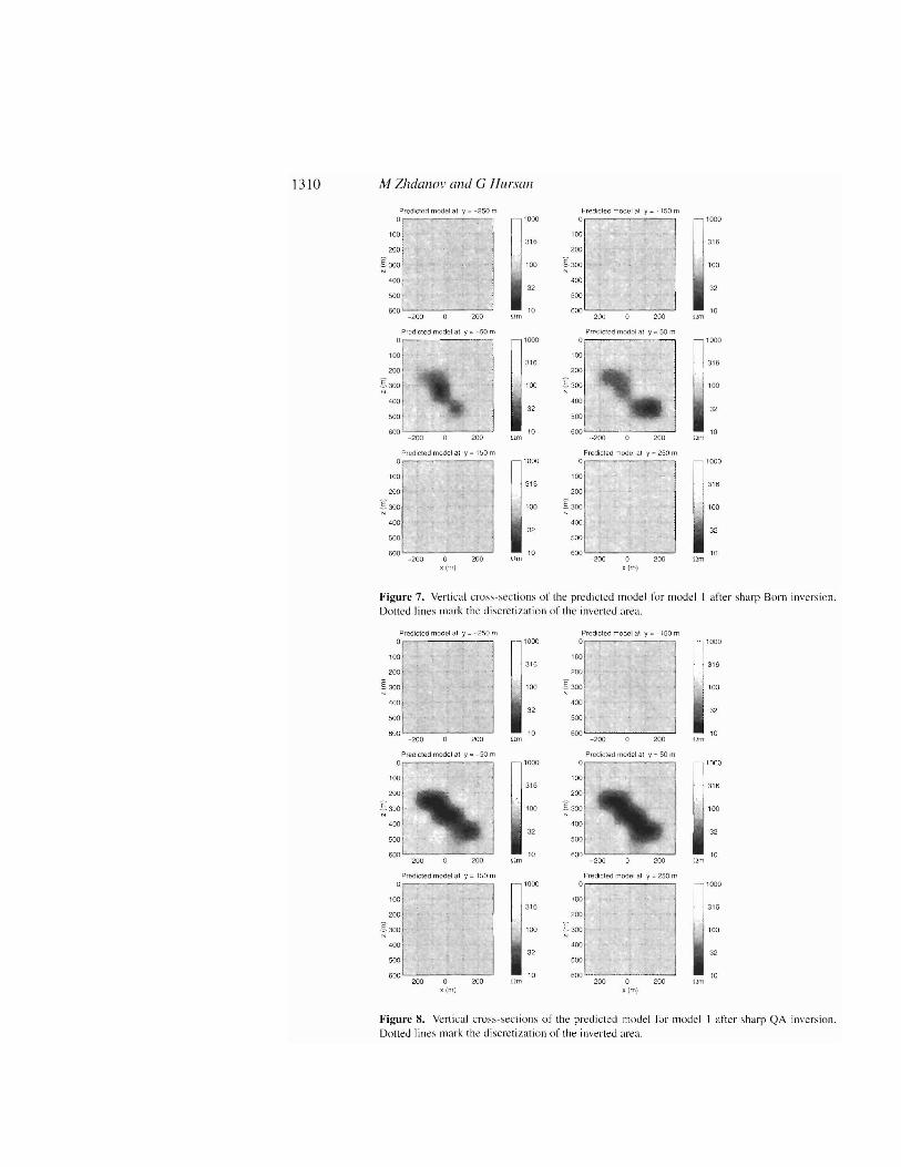
The differenc e between the QA and Born inversion becomes sig nificant if we use the sharp stabilizer, If we have a good es timatio n of the upp er and lower boundaries of the model parameters, using thi s stabilize r we ca n usuall y recover the geo metry of the anomalous struc ture with high resolution . A lso, this requi res a very accurate forward modelling as a basis for the inve rsion. The sha rp Born inversion gives an und erestimated size of the anoma ly (fig ure 7). The physical explanation for thi s is that. in the case of co nductive anomali es. the Bo rn approx imation gives higher field values tha n the exa ct solution. Therefore. an inver sion base d on this will underestimate the conduct ance or the ano ma ly. which corresponds to a sma ller size for the given conductivity.

The QA inver sion solves this probl em. It is based on a much more acc ura te forwa rd ope rator than the Born approx imatio n. Th e differ ence between the synthetic data co mputed by the QA approximation and full integral equat ion (IE) solution is less than the given noise level. Therefore. the Q A inver sion provides almos t perfect reconstruction of the give n model (figure S).

With a reason able es tima te of the noi se level , the stopping criteria of the inversio n ca n be assigned to the point where the re lative misfit is minimized to this error level. In our case. it was 3% . The re-w eighting in the shar p inversion causes an increment of the mi sfit. We rc-weight again only if the misfit drops to the give n noi se level or if the paramet ric functio na l increases due to the penalization .

131 2 M Zhdano v and G Hursan

True model at z - 50 m

0 0 01 40"1"

200 _I-200 I 400 • . .. .I

- 400 - 2 DO 0 200 400

True model at z -; 2S0 m

'

:;:1 - ,

I 200 I 400 L ­

-400 - 200 0 200 4()(]

True model at z = 450 m

200 400

True model at z = 150 m 'ooo r---- - ---- I ,----, 1000

-400 I . in316 I , 316

-2~)O l J 100 I I 100

132 . 32~O l I 400 I

10 -lim

Um

11m

10,...- 400 - 200 0 200 400

True model at z = 350 r-r 1000

- .

316r-~:;l ooo

316

-2:0 . : ~ 100 1 100

200 I

400

32 32

,10 -10

-4 00 - 200 0 200 400 11m

True model at z = 550 m 1000 '--- 11000- 400 f-' ------~ -'- -1 316 I I 316-200r . J

: , I 100 I I 100

. ! J>00 I32 .32

400 L _ ­10 - 10

- 400 - 200 0 200 400 llm

Figure In. Hori zont al cro ss-sec tions of the inverted area and the true model for model 2. Dot, show the locati on of receiver points, Dolled lines mark the discret iza tion of the inverted area.

Predicted mod el at z = 50 m Predicted mode l at z = 150 m

0

::1 o~. J ~:::n ::::63::L ',.. '. j U :: IL~

- I1. . . ~ 63 ;

40140 ~-~ O ~ 400 12m - 40 0 -2 00 0 ~ 4 00 11m

Predicted moc er at 7 '" 250 m Predicted model I'll 1 = 350 m 25 1 251

-400 - 400

- 200 158 - 200 158

o ~ : 100 0! 200 ~ 63 ?OO ~ 400 40 0

40 ...._--~~~---'

- 400 - 200 0 200 400 Urn ~ 400 - 200 0 200 400

Predicted moue! FIt z oo 450 m Predicted model al I '" 550 111

! [ 251 '--' , - 251j - 400 : ...:... 1 - 4oo i II ~.'- 200 156 - 200 \ " 5B

i100 0 I ','. 1::L: '~ ~ 63 ::1 -1100

"GJ

~ 40 ~ - 40 - 4 OO -200 0 200 400 urn -400 - 200 0 200 400 Um

Figure II. Hor izon tal cross-sec tions of the predicted model for mode l 2. after smooth Born inversion, Dots show the location of receiver poi nts. Dolled lines mar k the discre tization of the inverted area .

Quasi-analytical i Ill'£'rsion 13 13

PredICted model at z ;; sam PrediCled model HI 7 =. 150 m

J-~ 400 . - 200 .

o 200 ·

~

• •

•••

• •

. 1Ii

. :

•

n....25 1

I.rs

f',100

63

:::1. : ~. ' ..: . i ' .

200 L I,." : ::

100

63

400 · . . . 40 400 · : '~ 40

- 400 - 200 0 200 <tOO <1m - 400 - 200 0 200 400 urn

Preoic ted model at 7 '" ?SO In Predicted mode l at z = 350 m

-4001 ' M-4 001~~' I::: -200 1- 200 t _.

I

o . ~. :: 20 0 I 400 . 40

·100t. ,~J Urn- 400 - 200 C 200 400

Predicted model at z '" 450 m I I

- 400 J' ,- 200 ••

200

400 , -''- ­

- 400 - 200 0 200 400

Predic ted model at z = 550 m 251

-400 J" 158

-2 00

100

20063

400 40

~

Urn- 400 -200 0 200 400 - 400 - 200 o 200 400 ~

F i~lIre 12. Horizontal cross -sec tions ofthe pred icted mode l for model 2 after smooth QA inversion . Dots show the location of rece iver po ints. Dotted lines mark the dis cretizat ion of the inverted area .

~: : ,. ,:. ... . ~ ~ , . : : :: L:Jr-. O060 '0­1• • 4( " . .- ,.

o . 100 0 · .. . . . 200 . 32 200

400 . 400• • • • ~ 10 l -'­

- 400 - 200 0 200 toQO - 400 - 200 0 200 400llm

Predicted mooe! al z = 50 m Predicted model at L '" 150 m

<1m

~1

15B

' 00

63

~

25 1

1 ~

100

63

W

1000

316

100

3?

10

Predicted model at z = 250 m Predicted model at ? = 350 m

- 400 ~400 . . ,..'. 1000 I --.·_.. · ··~

1000

- 200 . . 3 16 - 200 .. t ... 316~ 100~' ~,

1

I' ' : ! 322: . . '~ j . 400 . . 400 •

•-- ' 10 . 10 - 400 - 200 0 ?OO 400 s..' - 400 - 200 0 200 400 Il m

Predicted mo del at z ;:o 450 m Predicted model at z = 500 rn

. ........,j ~'000 I- 400 ~400

, I 1 '000~ o I

316 - 200

-':OU:. : • : : : 100

I ?OO l •• ' 32

200 i • . 32

400 . 10

.00 1 ~ 00

- 400 - 200 0 200 400 Il m - 400 - 200 0 200 400 Il m

Fi~ urc 13. Horizontal cross-section s of the predicted model for model 2 after sharp 13 0m inversio n. Dots show the location of receiver point s. Dotted lines mark the discretization of the inverted area.

1314 M 7.Jula I101' lind G 1I1IrsGn

Predic ted rnooet at L '" 50 rn Pre dic ted mouet OI l I ~ 150 m

-400 I.. . . . - 200

200

400

- 400 -2 00 0 200 400

n100 0

3 16

jt 100

32

,... 10

Pre(J\\;led mo de l at z =250 m Predicte d mode l a~ z '" 350 m ' OOO

- 400 I ' ----'-' ~4 ()O " 1 I '000

- 200· 1 3

., 100

n' 6 - 200 1 • •

li316 , j 100

200 200 32 32 IW

1400 400 10 10

- 400 - 200 a 200 4()O "m - 400 - 200 a 200 400 llm

Preocteo mode l i'li 1 = 4~ m

r-----'" ­- 400 j

I - 200j •

o I 200 r 400 IL ,ftC

Predicted model at z ':: 550 m 100 0

3 16 I

:[J~: l ::" -: .:: I o .' 00

200 ' . 32

40 0 . .

10

100 0

316

too

32

10 - 400 - 200 a 200 400 11m -400 - 200 0 200 400 11m

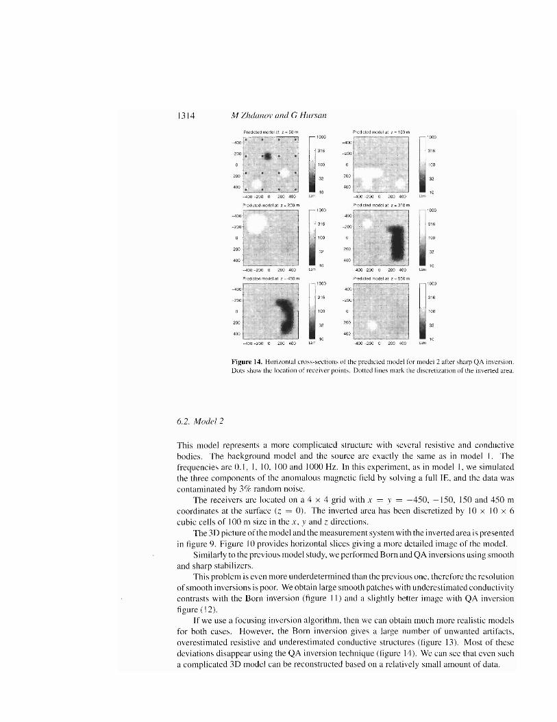
Figure 14. Horizont al cros s-se ctio ns of the predicted model for model 2 a fter sharp QA inversion. Dots show the location of rece iver poin ts. DOlled lines mark the d iscre tization of the inverted area .

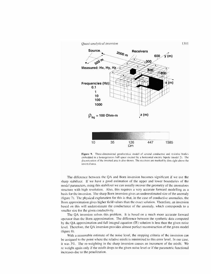
6.2. Model 2

Thi s model repre sent s a more complicated structure with several resistive and conductive bodies. The background model and the source arc exactly the sa me as in model I. The frequ encies arc O. L I, 10. 100 and 1000 Hz. In this experiment . as in model I. we simulated the three components of the anomalou s magnet ic field hy so lving a full IE. and the data was contaminated by 3% random noi se.

The receivers are located on a 4 x 4 grid with x = y = - 450. -150. 150 and 450 m coo rdinates at the surface (z = 0). The inverted area has been di scretized by lO x lO x 6 cubic cel ls of 100 m size in the x , y and z directions.

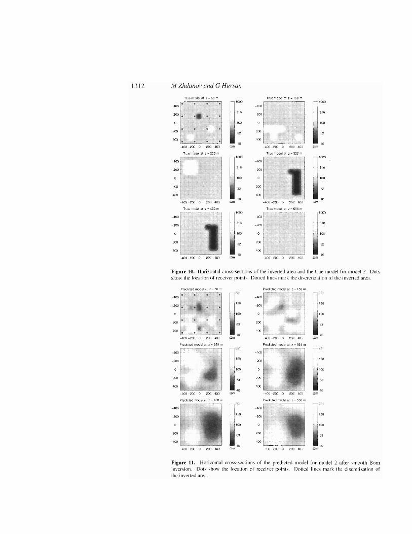
Th e 3D picture of the model and the measurement sys tem with the inverted area is presented in figure 9. fi gure 10 provides hori zontal slices giving a more detailed image of the model.

Similarly to the previ ous model study, we performed Born and QA inversions using smooth and sharp stabilizers.

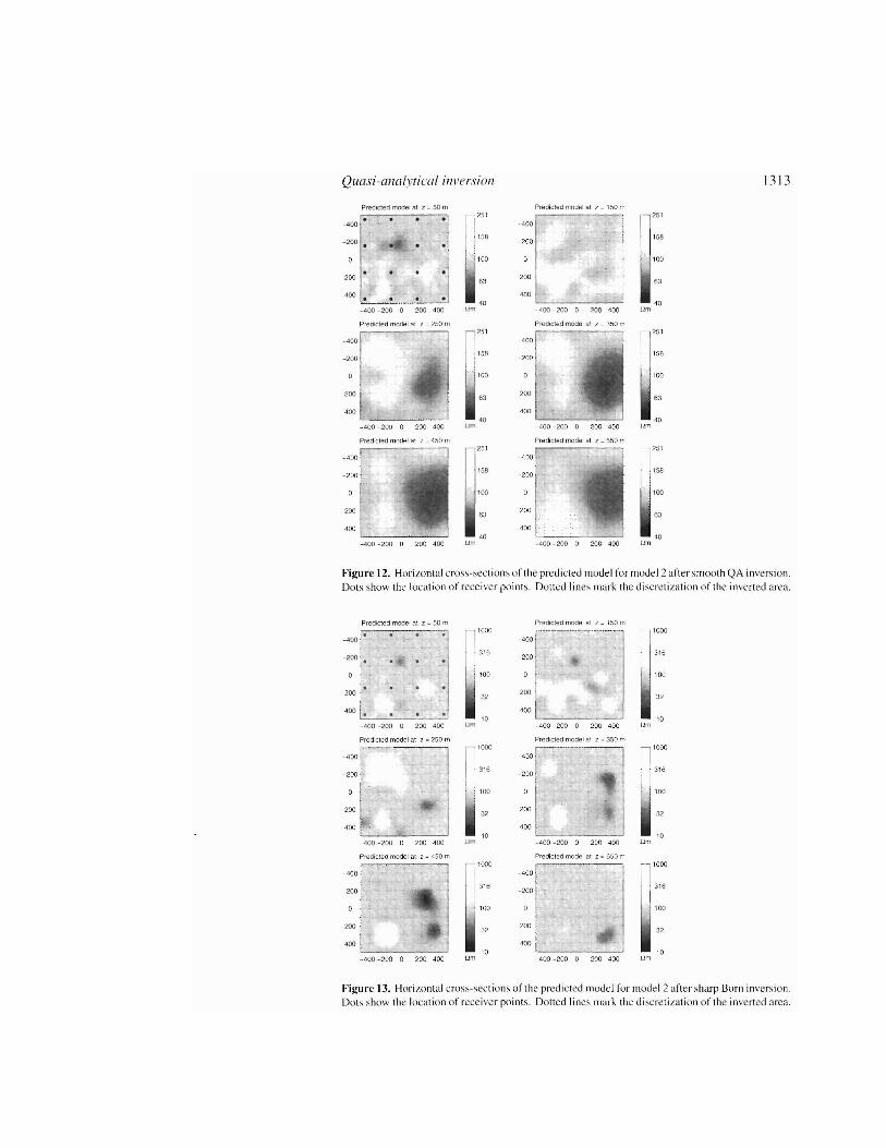
This prob lem is even more underdeterrn incd than the previous one, therefor e the resolution of smoo th inversions is poor. We obtain large smooth patches with underestimated co nductivity co ntrasts with the Born inversion (figure I I) and a slightly better image with QA inversion figure ( 12).

If we use a focusing inversion algorithm, then we can obtain much more realistic model s for both cases . However, the Born inversi on gives a large number of unwanted artifact s. overestimated resist ive and underestimated conductive structures (figure 13). Most of these devi ation s disappear using the QA invers ion technique (figure 14). We can see that even such a complicated 3D model can be reconstru cted based on a relati vely small amount of data.

1315 Quasi-analytical inversion

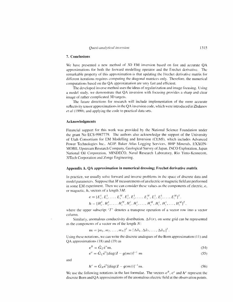
7. Conclusions

We have presented a new method of 3D EM inversion based on fast and accurate QA approximations for both the forward modelling operator and the Frechet derivative. The remarkable property of this approximation is that updating the Frechet derivative matrix for different iterations requires computing the diagonal matrices only. Therefore, the numerical computations based on the QA approximation are very fast and efficient.

The developed inverse method uses the ideas of regularization and image focusing. Using a model study, we demonstrate that QA inversion with focusing provides a sharp and clear image of rather complicated 3D targets.

The future directions for research will include implementation of the more accurate reflectivity tensor approximations in the QA inversion code, which were introduced in Zhdanov et al (1999). and applying the code to practical data sets.

Acknowledgments

Financial support for this work was provided by the National Science Foundation under the grant No ECS-9987779. The authors also acknowledge the support of the University of Utah Consortium for EM Modelling and Inversion (CEMI), which includes Advanced Power Technologies Inc .. AGIP, Baker Atlas Logging Services. BHP Minerals, EXXON­MOBIL Upstream Research Company, Geological Survey of Japan, INCa Exploration, Japan National Oil Corporation, MINDECO, Naval Research Laboratory, Rio Tinto-Kennecott, 3JTech Corporation and Zonge Engineering.

Appendix A. QA approximation in numerical dressing; Frechet derivative matrix

In practice, we usually solve forward and inverse problems in the space of discrete data and model parameters. Suppose that M measurements of an electric or magnetic field are performed in some EM experiment. Then we can consider these values as the components of electric, e, or magnetic, 11" vectors of a length 3M:

e = [E~, E;, £;\1. E;,. E; £;\11 , E;, E;, , E~] T•

h = [H), H;, H\M. H\I. H,I , H,M, H). H/ Htf, where the upper subscript' T' denotes a transpose operation of a vector row into a vector column.

Similarly, anomalous conductivity distribution, ,6.0- (r ), on some grid can be represented as the components of a vector tri of the length N:

m = [mI. lJl2•...• lJlNf = [,6.al. ,6.a2•... , ,6.aN f. Using these notations, we can write the discrete analogues of the Born approximation (11) and QA approximations (18) and (19) as

B e

A <b = GEe rn, (54)

ell = GEehrdiag(l- g(m))r l m (55)

and

h" = GHeh[diag(l- g(m))r1m. (56)

We use the following notations in the last formulae. The vectors en, e" and h" represent the discrete Born and QA approximations of the anomalous electric field at the observation points.

1316 M Zhdanov and c Hursan

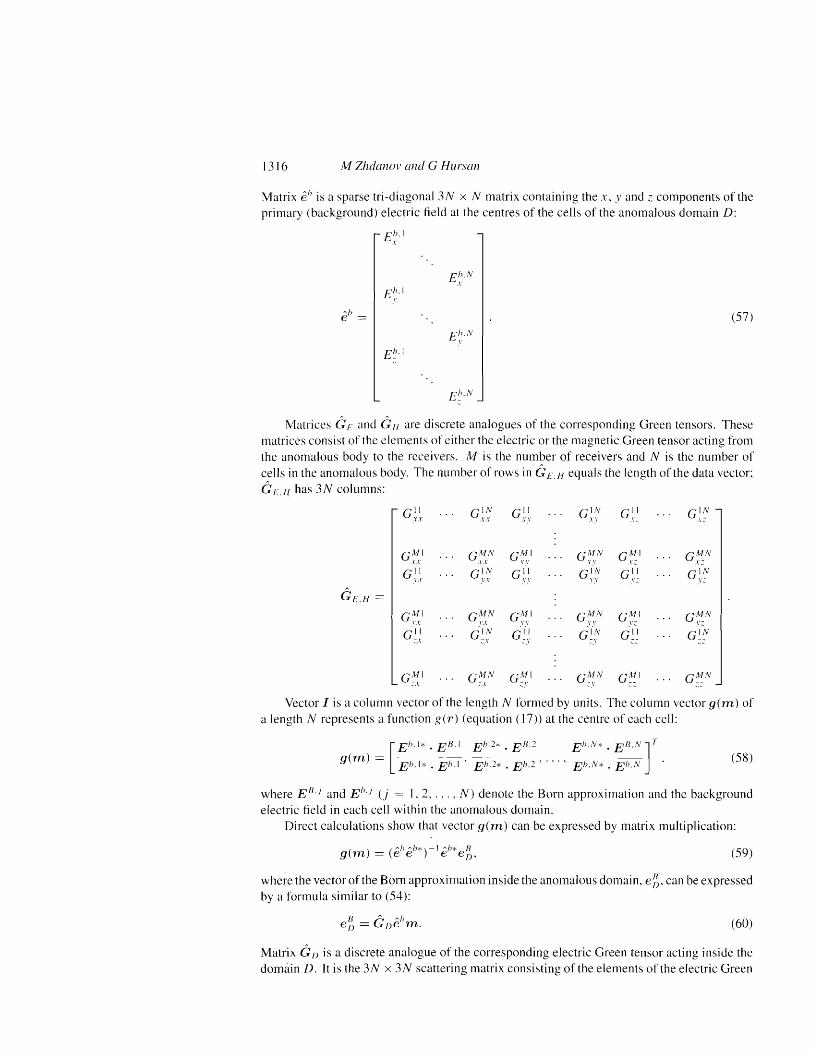
Matrix eh is a sparse tri-diagonal 3N x N matrix containing the x, y and z components of the primary (background) electric field at the centres of the cells of the anomalous domain D:

Eh,1 \

Eh,N x

Eh,1 I'

~h 1 I·e = (57) Eh,N

v

E~,I

Eh,N

Matrices GF. and G/I are discrete analogues of the corresponding Green tensors. These matrices consist of the elements of either the electric or the magnetic Green tensor acting from the anomalous body to the receivers. M is the number of receivers and N is the number of cells in the anomalous body. The number of rows in GE, H equals the length of the data vector; GE,H has 3N columns:

... . .. ell . .. IN G~.~ G~~ G~:, G:~ x; e .1 ;

G~l ... eAlN G~,I . .. elvIN G~I . .. eMN .1.1' \I x;

ell ... . .. . .. cv: e:,~ e" e~,~IX \'.1' e:~ v;

GE,H = I

... k/ l e~1 e~N e\'\

.. . e~N e~1 . .. e~N

... GIN . .. . .. e";.1' ;x e~.~, G~~ G~~ G~r:

Ml eMN e ;.\ ... e~1 . .. e~N e~!l . .. e~N

;x

Vector I is a column vector of the length N formed by units. The column vector gem) of a length N represents a function geT) (equation (17)) at the centre of each cell:

Eh, h . E R. I E h.2*. EB.2 Eh,N* • ER'N] T

gem) = , ~-')~--"') , ... , I (58)[ Eh.l* • Eh.1 e->, Eh,~ Eh,N* • E/7.l\

where EB.j and Eh,j (j = L 2.... , N) denote the Born approximation and the background electric field in each cell within the anomalous domain.

Direct calculations show that vector gem) can be expressed by matrix multiplication:

~ b ~ h* ) - I ~ fJ* R g (m ) = ( e e e e/). (59)

where the vector of the Born approximation inside the anomalous domain. eZ, can be expressed by a formula similar to (54):

B G~ ~h e/) = /)e m. (60)

Matrix GD is a discrete analogue of the corresponding electric Green tensor acting inside the domain D. It is the 3N x 3N scattering matrix consisting of the elements of the electric Green

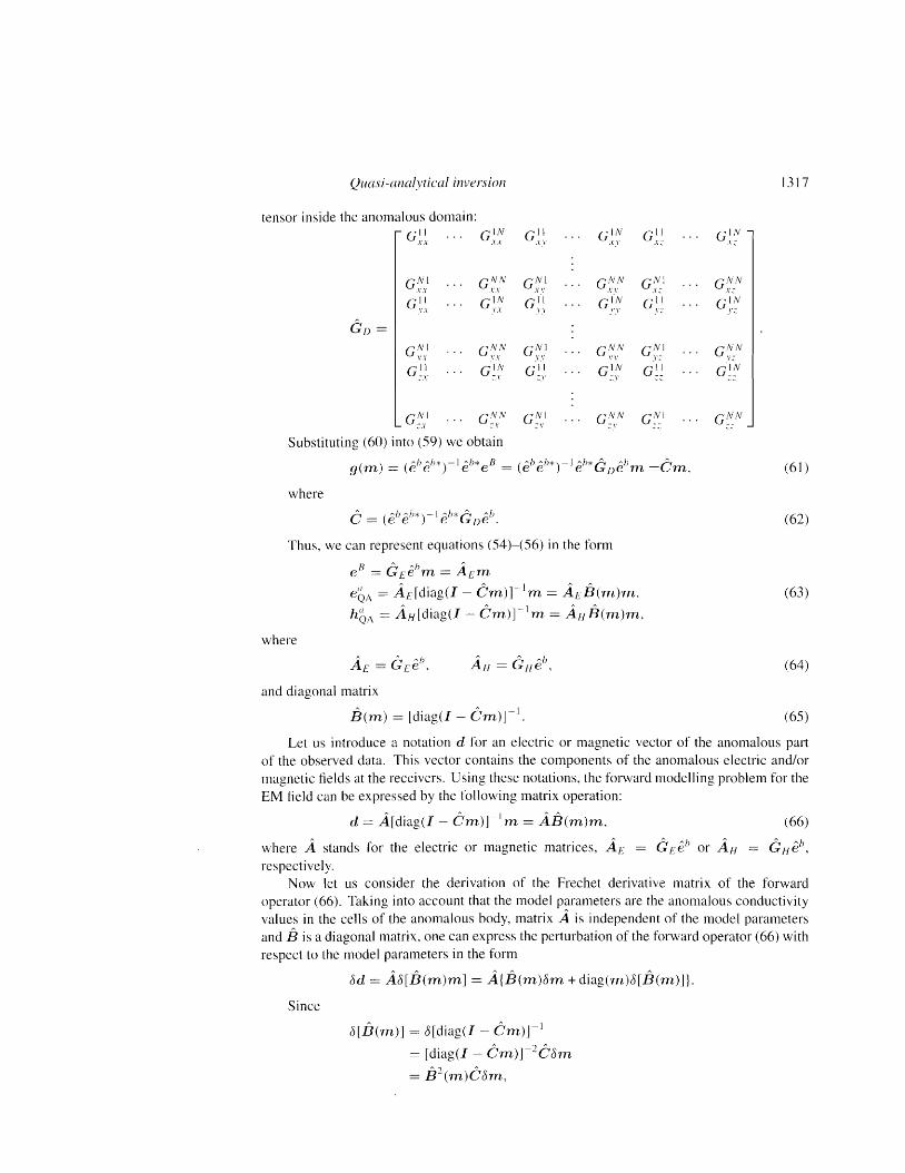
1317 Quasi-analytical inversion

tensor inside the anomalous domain: GIN GING,~_~ . . . G;~ G~;, .r v G_~~ v;

G~/ ... G NN n G~} G~\N GN!

,\ ;: GNN x;

G;,~ ... GIN YX

G(I vv G_;:~ G;~ GIN

y;

Gn =

G~\I ... G~t G~I'I G~t G~/ GNN yz

G~~ ... GIN ;,\ G~\I, G~~ G~~ G~;V

G NN G~I ... G~~N G~,I ;:I' c: G!,!N -Substituting (60) into (59) we obtain

g(m) = (eheh*)-Ieb*e B = (eheh*)-leh*Gnehm =Cm. (61 )

where

C = (eheh*)- I e')*GDeb. (62)

Thus, we can represent equations (54)-(56) in the form B <hA A

e = GEe m = AEm A A A AI

eOA= AEfdiag(I - Cm)r m = AcB(m)m. (63) A A A AI

hOA= AH[diag(I - Cm)r m = AHB(m)m.

where A A A AI I

A E = GEe). A H = GHe), (64)

and diagonal matrix

B(m) = [diag(I - Cm)r l . (65)

Let us introduce a notation d for an electric or magnetic vector of the anomalous part of the observed data. This vector contains the components of the anomalous electric and/or magnetic fields at the receivers. Using these notations, the forward modelling problem for the EM field can be expressed by the following matrix operation:

A A A AI d = A[diag(I - Cm)r m = AB(m)m. (66)

where A stands for the electric or magnetic matrices, A E = GEeb or A H = GHeb,

respectively. Now let us consider the derivation of the Frechet derivative matrix of the forward

operator (66). Taking into account that the model parameters are the anomalous conductivity values in the cells of the anomalous body, matrix A is independent of the model parameters and B is a diagonal matrix, one can express the perturbation of the forward operator (66) with respect to the model parameters in the form

8d = A8[B(m)m] = A{B(m)8m + diag(m)8[B(m)]}.

Since

8[B(m)] = 8[diag(I - Cm)r l

= [diag(I - Cm)r2C8m

= B 2(m)C8m.

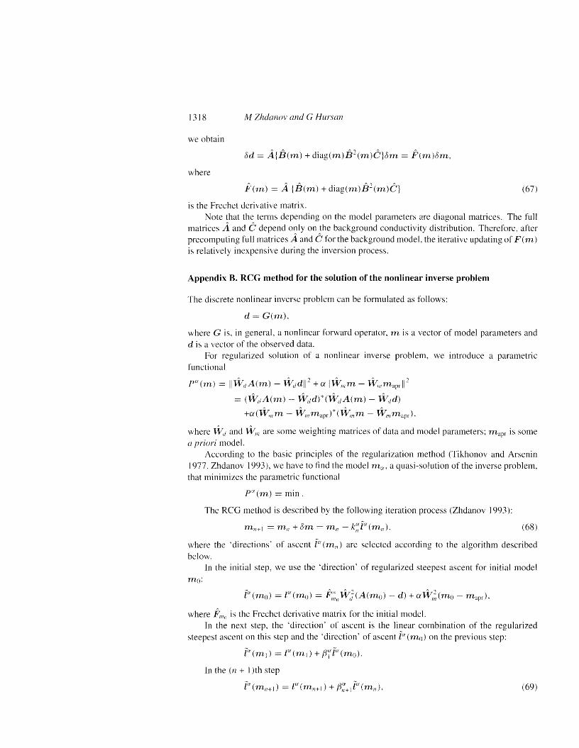
1318 M Zhdanov and G Hursan

we obtain

8d = A{B(1n) + diagCm)1}2(m)C}8m = F(m)8m,

where

F(m) = A {B(m) + diag(m)B2(m)C} (67)

is the Frechet derivative matrix. Note that the terms depending on the model parameters are diagonal matrices. The full

matrices A and C depend only on the background conductivity distribution. Therefore, after precomputing full matrices A and C for the background model, the iterative updating of F (m)

is relatively inexpensive during the inversion process.

Appendix B. ReG method for the solution of the nonlinear inverse problem

The discrete nonlinear inverse problem can be formulated as follows:

d = G(m),

where G is, in general, a nonlinear forward operator, m is a vector of model parameters and d is a vector of the observed data.

For regularized solution of a nonlinear inverse problem, we introduce a parametric functional

a 2 2A A A A

P (m) = IIWdA(m) - Wddll +allW;n m - W;nmaprll

= (l,vdA(m) - Wdd)*(~/A(m) - Wdd)

+a(l¥;n m -l¥;nmapr)*(-a~nm - Wmmapr ) ,

where Wi! and l¥;n are some weighting matrices of data and model parameters; m apr is some a priori model.

According to the basic principles of the regularization method (Tikhonov and Arsenin 1977, Zhdanov 1993), we have to find the model nta , a quasi-solution of the inverse problem, that minimizes the parametric functional

pCl(m) = min.

The ReG method is described by the following iteration process (Zhdanov 1993):

m n+l = m n + om = m n - k~fCl(mn), (68)

where the 'directions' of ascent [a (mn ) are selected according to the algorithm described below.

In the initial step, we use the 'direction' of regularized steepest ascent for initial model mo:

fa(mo) = [CI(mo) = F;oWj(A(mo) -- d) +alV;~(mo - m apr),

where F,no is the Frechet derivative matrix for the initial model. In the next step, the 'direction' of ascent is the linear combination of the regularized

steepest ascent on this step and the 'direction' of ascent fCi (mo) on the previous step:

fCl(m]) = [CI(m)} + f3f fa (m o).

In the (n + I )th step

fCi (mn+l) = [CI (mn+l) + f3~+JCI (mn ) , (69)

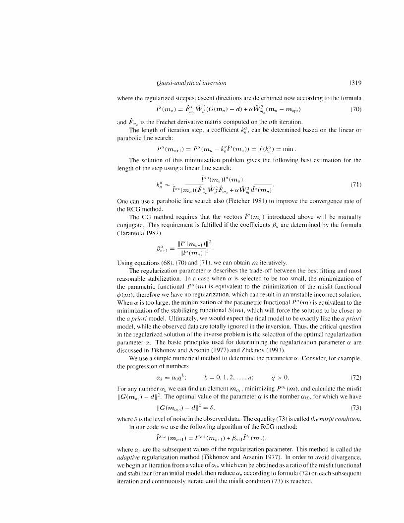
1319 Quasi-analytical inversion

where the regularized steepest ascent directions are determined now according to the formula

la(mn) = F;~IIW}(G(rnll) - d) +a~~II(rnll - m apr ) (70)

and F,1l is the Frechet derivative matrix computed on the nth iteration. 11

The length of iteration step, a coefficient k~, can be determined based on the linear or parabolic line search:

pU(mn+l) = P''Lrn; - k~ilX(rnn» = f(k~) = min.

The solution of this minimization problem gives the following best estimation for the length of the step using a linear line search:

fIX *(m )iCY (m )n n k~ = A A,., A A _ • (71 ) _

la* (rnn )(F,~II W:7 F,nll

+ a lV;~ )la (rrt ll )

One can use a parabolic line search also (Fletcher 1981) to improve the convergence rate of the RCG method.

The CG method requires that the vectors ilX (mil) introduced above will be mutually conjugate. This requirement is fulfilled if the coefficients f3n are determined by the formula (Tarantola 1987)

IllU (rrt l1 + 1)11

2

f31~+1 2Illa(rnn)11 .

Using equations (68), (70) and (71), we can obtain m iteratively. The regularization parameter a describes the trade-off between the best fitting and most

reasonable stabilization. In a case when a is selected to be too small, the minimization of the parametric functional P" (rrt) is equivalent to the minimization of the misfit functional ¢(rn); therefore we have no regularization, which can result in an unstable incorrect solution. When a is too large, the minimization of the parametric functional P" (m) is equivalent to the minimization of the stabilizing functional SCm), which will force the solution to be closer to the a priori model. Ultimately, we would expect the final model to be exactly like the a priori model, while the observed data are totally ignored in the inversion. Thus, the critical question in the regularized solution of the inverse problem is the selection of the optimal regularization parameter a. The basic principles used for determining the regularization parameter a are discussed in Tikhonov and Arsenin (1977) and Zhdanov (1993).

We use a simple numerical method to determine the parameter a. Consider, for example, the progression of numbers

ak = aoqk: k = 0, 1,2, ... , n; q > O. (72)

For any number a; we can find an element rrta ! , minimizing PU! (m). and calculate the misfit IIC(mu!) - d11 2 . The optimal value of the parameter a is the number akO, for which we have

IIC(ma!IJ) - dl1 2 = 8. (73)

where 8 is the level of noise in the observed data. The equality (73) is called the misfit condition. In our code we use the following algorithm of the RCG method:

i-» (mn+l) = lU II + 1(mn+l) + f311+JIX II (mn ) .

where an are the subsequent values of the regularization parameter. This method is called the adaptive regularization method (Tikhonov and Arsenin 1977). In order to avoid divergence, we begin an iteration from a value ofao, which can be obtained as a ratio of the misfit functional and stabilizer for an initial model, then reduce an according to formula (72) on each subsequent iteration and continuously iterate until the misfit condition (73) is reached.

1320 M Zhdanov and G Hursan

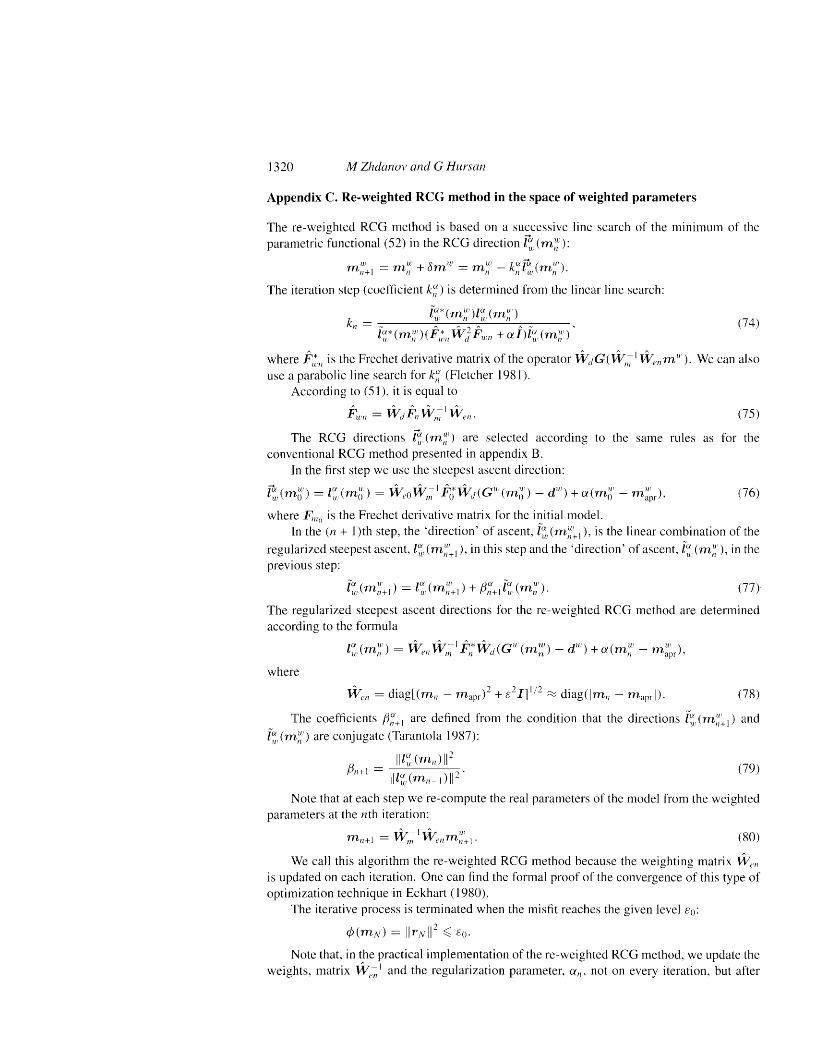
Appendix C. Re-weighted RCG method in the space of weighted parameters

The re-weighted RCG method is based on a successive line search of the minimum of the parametric functional (52) in the RCG direction ~,(m~}):

UJ U 1 11) U,I a a 11) m n+1 = m n + 8m = m n - knlw(mn).

The iteration step (coefficient k~) is determined from the linear line search:

l~]* (m;;J)l~ (m~)) (74)k; = - . A A 2 A A - .'

l~}*(m~')(Fl7,1lW d Fum + (1)l~,(m~')

where Fl: n is the Frechet derivative matrix of the operator WdG(lV;;;-1 Wenm U ' ) . We can also

use a parabolic line search for k~ (Fletcher 1981). According to (51), it is equal to

-1A A A A A

Fum = WdFn w; Wen. (75)

The RCG directions ~, (m;n are selected according to the same rules as for the conventional RCG method presented in appendix B.

In the first step we use the steepest ascent direction: a w a 11) A" - J A * A 11) 11) lL' til 11)lw(mo ) = lw(mo ) = W eOliV,n Ft) Wd(G (mO ) - d ) + a(mO - m apr)' (76)

where F,no is the Frechet derivative matrix for the initial model. In the (n + l)th step, the 'direction' of ascent, i~/m:+,), is the linear combination of the

regularized steepest ascent, l~) (m~~ I)' in this step and the'direction' of ascent, i~) (m~'), in the previous step:

-Cl' ( U') laC W) f3Cl'l-a( W)l w m n+ 1 = w m n+ 1 + n+ I w m n . (77)

The regularized steepest ascent directions for the re-weighted RCG method are determined according to the formula

d Wl~](m:) = Wen Wn~1 i;;Wd(GW(m~) - ) + a(m~' - m~~r)'

where

Wen = diagjtrn, - m apr)2 + 8 21]1/2 ~ diagtjrn; - maprl). (78)

The coefficients f3~+1 are defined from the condition that the directions i; (m~~l) and

i~](m~') are conjugate (Tarantola 1987):

_ Ill~,(mn) f 79 f3n+1 - Ill~(mn_])112 ( )

Note that at each step we re-compute the real parameters of the model from the weighted parameters at the nth iteration:

A A-I W

m n+l w; W enmn+ 1 • (80)

We call this algorithm the re-weighted RCG method because the weighting matrix Wen is updated on each iteration. One can find the formal proof of the convergence of this type of optimization technique in Eckhart (1980).

The iterative process is terminated when the misfit reaches the given level 80:

¢(mN) = IIrNI12 ~ 80.

Note that, in the practical implementation of the re-weighted RCG method, we update the weights, matrix W -;; 1 and the regularization parameter, an, not on every iteration, but after e

1321 Quasi-analytical inversion

performing a sequence of iterations (usually five or ten) with the fixed values of We-;;(~ and ano' This improves the convergence rate and robustness of the algorithm, keeping the value of the regularization parameter (XII from being too small during the iteration process.

Numerical tests show that the MS functional generates a stable solution but it tends to produce the smallest possible anomalous domain. Following Portniaguine and Zhdanov (1999), we now impose the upper boundary ~a+(r) and the lower boundary ~a-(r) for the conductivity values ~a(r) determined as a result of inversion. During the iterative process we simply cut off all the values outside these boundaries. This algorithm can be described by the following formula:

~a(r) = ~a+(r), if ~a(r) ;? ~a+(r) (81 )

~a(r) = ~a-(r), if ~a(r) ~ ~a-(r).

Thus, according to the last formula the anomalous conductivities ~a (r) are always distributed within the interval

~a-(r) ~ ~a(r) ~ ~a+(r).

References

Alumbaugh D L and Newman G A 1997 Three-dimensional massively parallel inversion II. Analysis of a cross-well electromagnetic experiment Geophvs. 1. Int. 128355-63

Avdeev D, Kuvshinov A, Pankratov 0 and Newman G A 1998 Three-dimensional frequency domain modelling of airborne electromagnetic responses Exploration Geophvs. 29 111-19

Berdichevsky M Nand Zhdanov M S 1984 Advanced Theon ofDeep Geomagnetic Sounding (Amsterdam: Elsevier) Born M 1933 Optics (Berlin: Springer) Constable S C. Parker R C and Constable G G 1987 Occam's inversion: a practical algorithm for generating smooth

models from EM sounding data Geophysics 52 289-300 Dmitriev V I and Pozdnyakova E E 1992 Method and algorithm for computing the EM field in a stratified medium

with a local inhomogeneity in an arbitrary layer Comput. Math. 3 181-8 Druskin V. Knizhnerman L and Lee P 1999 New spectral Lanczos decomposition method for induction modelling in

arbitrary 3D geometry Geophysics 64 701-6 Eaton P A 1989 3D EM inversion using integral equations Geophys. Prosp. 37407-26 Eckhart L 1980 Weber's problem and Weiszfelds algorithm in general spaces Math. Programming 18 186-208 Fletcher R 1981 Practical Methods of Optimization (New York: Wiley) Golubev N. Zhdanov M S. Matsuo K and Negi T 1999 Three-dimensional inversion of magnetotelluric data over

Minami-Noshiro oil field Proc. 2nd Int. Symp. of Three-Dimensional Electromagnetics 1999 (Salt Lake City,

ur, pp 305-8 Habashy T M. Chew W C and Chow E Y 1986 Simultaneous reconstruction of permittivity and conductivity profiles

in a radially inhomogeneous slab Radio Sci. 21 635-45

Habashy T M. Groom R Wand Spies B R 1993 Beyond the Born and Rytov approximations: a nonlinear approach to electromagnetic scattering 1. Geophvs. Res. 98 1759-75

Hohmann G W 1975 3D induced polarization and EM modelling Geophvsics 40 309-24 Lee K Hand Xie G 1993 A new approach to imaging with low frequency EM fields Geophysics 58 780-96 Madden T R and Mackie R L 1989 3D magnetotelluric modelling and inversion Proc. IEEE 77 318-32 Mehanee S. Golubev Nand Zhdanov M S 1998 Weighted regularized inversion of magnetotelluric data Expanded

Abstracts SEG 68th Annual Meeting (New Orleans) pp 481-4 Nekut A 1994 EM ray-trace tomography Geophysics 59 371-7 Newman G A and Alumbaugh D L 1997 Three-dimensional massively parallel inversion: I. Theory Geophvs. J. Int.

128355-63 Oristaglio M, Wang T, Hohmann G Wand Tripp A 1993 Resistivity imaging of transient EM data by conjugate-gradient

method SEG Abstracts (Washington DC: SEG) pp 347-50 Oristaglio M L 1989 An inverse scattering formula that uses all the data Inverse Problems 51097-105 Pellerin L. Johnston J and Hohmann G W 1993 3D inversion of EM data SEG Abstracts (Washington, DC: SEG)

pp 360-63 Portniaguine 0 and Zhdanov M S 1999 Focusing geophysical inversion images Geophysics 64 874-87 Rudin L l, Osher Sand Fatemi E 1992 Nonlinear total variation based noise removal algorithms Physico D 60 259-68

1322 M Zhdanov and G Hursan

Smith J T and Booker J R 1991 Rapid inversion of 2 and 3D magnetotelluric data 1. Geophvs. Res. 963905-22 Tarantola A 19~O Inverse Problem Theory (Amsterdam: Elsevier)

Tikhonov A Nand Arsenin V Y 1977 Solution of Ill-Posed Problems (New York: Winston and Sons)

Torres-Verdin C and Habashy T M 1994 Rapid 2.5-dimensional forward modelling and inversion via a new nonlinear

scattering approximation Radio Sci. 29 1051-79

Vogel C R and Oman M E 1998 A fast robust total-variation based reconstruction of noisy. blurred images IEEE

Trans. Image Processing 7 813-24 Wannamaker P E 1991 Advances in 3D magnetotelluric modelling using integral equations Geophvsics 56 1716-28

Weide It P 1975 EM induction in 3D structures.l. Geophvs. 41 85-109 Xie G and Lee K H 1995 Nonlinear inversion of 3D EM data PIERS Proc. The Universits of Washington p 323 Xiong Z 1992 EM modelling of 3D structures by the method of system iteration using integral equations Geophysics

57 1556-61

Zhdanov M S 1993 Tutorial: Regularitation in Inversion Theon' (Colorado School of Mines) p 47

Zhdanov M S. Dmitriev V r. Fang Sand Hursan G 1999 Quasi-analytical approximations and series in electromagnetic

modelling Geophysics at press Zhdanov M S and Fang S 1996a Quasi-linear approximation in 3D EM modelling Geophvsics 61 646-65

--1996b 3D quasi-linear EM inversion Radio Sci. 31 741-54 --1997 Quasi linear series in 3D EM modelling Radio Sci. 322167-88 --1999 3D quasi-linear electromagnetic modelling and inversion Three Dimensional Electromagnetics (SEG

Monograph) (Tulsa. OK: SEG) pp 233-55

Zhdanov M S and Keller G 1994 The Geoelectrical Methods in Geophvsical Exploration (Amsterdam: Elsevier) p 873