NUMERICAL MODELING AND INVERSION OF GEOPHYSICAL ELECTROMAGNETIC MEASUREMENTS USING A THIN PLATE MODEL

MARKKUPIR TTIJÄRVI

Department of Geosciences,Division of Geophysics,

University of Oulu

OULU 2003

MARKKU PIRTTIJÄRVI

NUMERICAL MODELING AND INVERSION OF GEOPHYSICAL ELECTROMAGNETIC MEASUREMENTS USING A THIN PLATE MODEL

Academic Dissertation to be presented with the assent ofthe Faculty of Science, University of Oulu, for publicdiscussion in Raahensali (Auditorium L10), Linnanmaa, onNovember 8th, 2003, at 12 noon.

OULUN YLIOPISTO, OULU 2003

Copyright © 2003University of Oulu, 2003

Reviewed byProfessor Laust B. PedersenProfessor Peter Weidelt

ISBN 951-42-7119-X (URL: http://herkules.oulu.fi/isbn951427119X/)

ALSO AVAILABLE IN PRINTED FORMATActa Univ. Oul. A 403, 2003ISBN 951-42-7118-1ISSN 0355-3191 (URL: http://herkules.oulu.fi/issn03553191/)

OULU UNIVERSITY PRESSOULU 2003

Pirttijärvi, Markku, Numerical modeling and inversion of geophysicalelectromagnetic measurements using a thin plate model Department of Geosciences, Division of Geophysics, University of Oulu, P.O.Box 3000, FIN-90014University of Oulu, Finland Oulu, Finland2003

Abstract

The thesis deals with numerical methods designed for the modeling and inversion of geophysicalelectromagnetic (EM) measurements using a conductive thin plate model. The main objectives are tostudy the EM induction problem in general and to develop practical interpretation tools for mineralprospecting in particular.

The starting point is a linearized inversion method based on the singular value decomposition anda new adaptive damping method. The inversion method is introduced to the interpretation of time-domain EM (TEM) measurements using a thin plate in free-space. The central part of the thesis is anew approximate modeling method, which is based on an integral equation approach and a speciallattice model. At first the modeling method is applied to the interpretation of frequency-domain EM(FEM) data using a thin plate in conductive two-layered earth. After this time-domain responses aremodeled applying a Fourier-sine transform of broadband FEM computations.

The results demonstrate that the approximate computational method can model the geophysicalfrequency and time-domain EM responses of a thin conductor in conductive host medium withsufficient accuracy, and that the inversion method can provide reliable estimates for the modelparameters. The fast forward computation enables interactive interpretation of FEM data and feasibleforward modeling of TEM responses. The misfit function mapping and analysis of the singular valuedecomposition have provided additional information about the sensitivity, resolution, and thecorrelation behavior of the thin plate parameters.

Keywords: direct problem, inverse problem, mineral exploration, three-dimensionalmodels

Acknowledgements

The studies for this PhD thesis were carried out during 1996-2003 and supported financially by the Academy of Finland (NOIGEM and IPEG projects), Outokumpu Mining Oy (the ‘GeoNickel’ research project funded by European Commission), Outokumpu Foundation, and Tauno Tönning Foundation.

This work would not have been possible without the help of others. I express my deepest gratitude to professor Sven-Erik Hjelt for supervising the work and managing the various projects I worked for. The inspiring impact of Dr Saurabh K. Verma (Hyderabad, India) especially at the early stage of this work is gratefully acknowledged. I thank Aimo Hattula and Risto Pietilä (Outokumpu Mining Oy) for their invaluable assistance in the EMPLATES development. I thank professors Pertti Kaikkonen, Markku Peltoniemi, Laust B. Pedersen, and Peter Weidelt for reviewing the original manuscript and for the many advice. I also thank my colleagues at the University of Oulu, the Geological Survey of Finland, and elsewhere for the collaboration and the many fruitful discussions. I'm grateful to Ms Tarja Tolvanen for the language review. Last but not least, I address my special thanks to my family, my friends, and Tea.

List of original papers

This thesis is based on three original papers and a manuscript that are referred to in the text by their Roman numeral:

I Pirttijärvi M, Verma SK and Hjelt S-E (1998): Inversion of transient electromagnetic profile data using conductive finite plate model. Journal of Applied Geophysics, 38: 181-194.

II Pirttijärvi M, Pietilä R, Hattula A and Hjelt S-E (2002): Modelling and inversion of electromagnetic data using an approximate plate model. Geophysical Prospecting, 50: 425-440.

III Hjelt S-E and Pirttijärvi M (2000): Some characteristics of the conducting plate model in the inversion of geophysical electromagnetic data. Inverse Problems, 16: 1209-1223.

IV Pirttijärvi M: Analysis of thin plate parameters in electromagnetic inversion. Manuscript to be submitted.

Contents

Abstract Acknowledgements List of original papers Contents 1 Introduction.................................................................................................................. 11

1.1 Background............................................................................................................. 11 1.2 Modeling and inversion methods............................................................................12 1.3 Thin plate model .....................................................................................................14 1.4 The structure of the thesis .......................................................................................15

2 Principles of electromagnetic methods ........................................................................16 2.1 Theory.....................................................................................................................16 2.2 Applications ............................................................................................................17

3 Numerical algorithms ..................................................................................................20 3.1 The adaptive damping method................................................................................20 3.2 The approximate thin plate modeling method ........................................................23

4 Analysis of the inversion characteristics......................................................................26 4.1 Misfit function mapping .........................................................................................27

5 Discussion and conclusions .........................................................................................32 References Appendix

1 Introduction

1.1 Background

Electromagnetic (EM) methods utilizing controlled sources have traditionally been used in near-surface geophysical investigations such as mineral and hydrocarbon exploration as well as in geological mapping and structural studies. Recently, the EM methods have become popular in environmental, archeological, and engineering investigations. Although the earliest geophysical EM systems were developed in the 1920's, the main thrust in theoretical and practical development was experienced after the World War II (Ward 1980). Since then numerous applications including surface, airborne, borehole, and underwater measurement systems have been developed. Before the advances in computer technology in the late 1960's, however, the interpretation of the EM measurements was based mainly on theoretical deductions and empirical observations, as well as on few analytical solutions and small-scale model studies. The development of numerical modeling methods during the last three decades has made it possible to realize the full three-dimensional (3-D) EM induction problem and to model more realistic geological structures. Moreover, the combined use of numerical modeling and inversion methods has enabled computerized quantitative interpretation of EM measurements.

In the case of inductive EM methods that are studied in this work, the dominant petrophysical parameter is the electrical conductivity (or its reciprocal, the resistivity), which represents the ability of electric charges to move inside a matter. Certain geological targets, such as graphite bearing schist zones and massive sulphide ore bodies, can produce a strong anomalous EM response, because their conductivity is considerably higher than the conductivity of the host rocks surrounding them. The aim of geophysical interpretation is to invert the measured EM data into knowledge about the spatial distribution of conductivity inside the earth, and to use that information in geological interpretation. Unfortunately, the inverse problem does not have a unique solution, because conductivity is a complex, continuous function and the data is collected using finite sampling (Hohmann & Raiche 1988). Therefore, direct inversion of EM data is not possible in practice. Although informative depth sections of the subsurface can be generated using transformation and imaging techniques, these qualitative methods cannot provide actual conductivity values. For quantitative interpretation, the geophysicists must use mathematical models to represent the geological conductivity structures. The

12

prerequisite is a theoretical forward solution to the EM induction problem that allows developing a numerical algorithm to compute the synthetic EM response of the selected model.

1.2 Modeling and inversion methods

The one-dimensional, horizontally layered earth is still one of the most useful models in geophysics. Analytical EM solutions for the layered earth model were developed already in the 1950's (Ward 1980). Solutions for several EM systems above a conductive half-space and layered earth can be found in Ward & Hohmann (1988) and Spies & Frischknecht (1991), for example. Analytical solutions are extremely important not only because they are needed in some multi-dimensional numerical modeling methods, but also because they can be used to verify the validity of other numerical algorithms. 1-D models, however, are not appropriate if the conductivity changes laterally. When considering an isolated conductive target in resistive surroundings, parametric models such as a half-plane, a sphere, and a rectangular plate in free-space (e.g., Grant & West 1965, Nabighian 1970, and Annan 1974) have been found very useful in geophysical interpretation. The problem with these methods is that in practice the conductive host rocks and overburden layer can modify the measured EM response considerably. The first numerical algorithms that used 2-D models and took the finite conductivity of the host medium into account were introduced in the late 1960’s and early 1970’s (e.g., Parry 1969, Coggon 1971, and Hohmann 1971). The first numerical solutions for fully 3-D EM problems appeared in the mid-1970's (Raiche 1974, Hohmann 1975, and Weidelt 1975). During the last 25 years the research has been intense and several advanced numerical solution methods have been developed. These include the papers of Wannamaker et al. (1984), Newman et al. (1986), Newman & Hohmann (1988), Lee et al. (1989), Xiong (1992), Wang & Hohmann (1993), Mackie et al. (1993), Torres-Verdín & Habashy (1994), Zhdanov & Fang (1996), Liu & Lamontage (1998), Mitsuhata (2000), and Sasaki (2001), to name but a few. For more detailed information, Hohmann (1988) provides an excellent introduction to numerical EM modeling. More recent reviews of numerical modeling methods are given in the papers of Raiche (1994) and Christensen (1997) and in the book of Oristaglio & Spies (1999).

The 2-D and 3-D numerical solution methods are mostly based on integral equation (IE) and differential equation (DE) approaches (Hohmann 1988). The IE methods can further be divided into surface and volume IE methods, while the two main classes of the DE methods are the finite-element and the finite-difference methods. Hybrid methods that use integral equations to solve the boundary conditions outside the target area and differential equations to solve the EM fields inside the conductive target, have also been developed (e.g., Lee et al. 1981). Although the IE methods are mathematically more demanding to formulate, they often suit the 3-D modeling better than the DE methods, because the EM fields need to be solved only inside the anomalous conductors (Hohmann 1988). Thus, the 3-D IE methods require less computer memory and computation time because the dimension of the resulting matrix system is generally much smaller. The DE

13

methods, however, suit the modeling of complex conductivity structures much better, because the IE methods are restricted to using horizontally layered host medium (Hohmann 1988). Furthermore, the DE methods can handle large conductivity contrasts better, especially when considering controlled source applications (Hohmann 1988). The finite-difference method provides also a convenient way to compute the partial derivatives for the inverse solution (Hohmann & Raiche 1988). No matter what solution method is used, accurate 3-D numerical EM modeling requires lots of computer resources and time because the increasing accuracy needs denser discretization that results in a larger matrix equation.

The computational requirements increase drastically when inversion or optimization methods are combined with the 3-D modeling. The aim of numerical inversion is to find the parameters of the best fitting model that produce the smallest misfit (or error) between the computed response and the measured data. The inversion methods are usually classified into local and global methods. For example, the steepest descent, conjugate gradient, and linearized least-squares inversion algorithms are local optimization methods, and the grid search, random search, simulated annealing, and neural network algorithms are global optimization methods. The biggest difference between the two is that the global methods search the parameter space more comprehensively for the optimal model. Therefore, global methods are likely to resolve the true minimum among possible local minimums better than local optimization methods, especially when the number of optimized parameters is large. Successful application of local optimization methods depends greatly on the proper selection of initial model parameters. However, local optimization methods are usually much faster than global methods because they do not require as many forward computations. More detailed information on geophysical inversion practices can be found from Lines (1988), Hohmann & Raiche (1988), Sen & Stoffa (1995) and Oristaglio & Spies (1999).

14

1.3 Thin plate model

Fig. 1. Schematic view of a thin conductive plate below conductive overburden.

The thin plate model is an extremely useful special case of a 3-D model because it can be used to represent many geologically and economically interesting conductive targets that appear as intrusive dipping dikes or nearly horizontal layers of finite size. In this thesis the main application of the thin plate model is in the prospecting of base metal (e.g., Ni, Cu, Zn) mineral deposits that often appear as isolated massive sulphide ore bodies. Fig. 1 shows a schematic view of a thin plate model in the lower part of a two-layered host medium. In the rectangular coordinate system the plane z=0 represents the earth's surface and the x and y coordinates refer to the geographical coordinates (north and east). The position of the plate is defined by the x, y, and z coordinates of the center of the upper side of the plate. One side of the plate is always parallel to the surface, and the orientation of the plate is defined by the (vertical) dip angle and the (horizontal) strike angle. The size of the plate is defined by the strike length, which is the plate width along the strike direction, and depth extent, which is the plate height along the dipping side of the plate. Because the plate is considered to be thin, its thickness and conductivity are strongly correlated and cannot be determined separately. Therefore their product, the conductance, is used to characterize the electrical property of the thin conductor. The two-layered host medium is defined by the resistivity of the host rock, in which the plate model is located, and the thickness and the resistivity of the overburden layer, which represents superficial till and sedimentary deposits, for example.

Layer resistivity (RL)Layer thickness (TL) Host resistivity (RH)

Depth of burial(DB)

Depth extent (DE)

X-position(XP)

Strike length(SL)

Y-position(YP)

Strikeangle(SA)

y

x

Conductance (CO)

-z

Dip angle(DA)

15

1.4 The structure of the thesis

This thesis is based on four publications that deal with the modeling and inversion of EM data using thin conductive plate model.

Paper I handles the inversion of time-domain electromagnetic (TEM) measurements using a thin plate model in free-space and introduces a linearized inversion scheme based on the singular value decomposition (SVD) and a new adaptive damping method. Inversion results with synthetic and field data are used to assess the validity of the optimization method.

Paper II describes an approximate numerical modeling method, which is used to model and to interpret frequency-domain EM (FEM) data using a thin plate in conductive two-layered host medium. Paper II exhibits forward computation results and inversion examples with synthetic data and field measurements.

Paper III reviews the EM inversion studies carried out at the University of Oulu. It addresses the role of misfit function mapping and SVD analysis when studying the parameters of the thin plate model.

Paper IV describes a revised version of the approximate modeling method and a transformation method that is used to compute time-domain EM responses from broadband frequency-domain results. The paper compares FEM and TEM inversions and uses the SVD information to analyze the inversion characteristics of the thin plate model.

The thesis synopsis provides the reader with relevant background information and briefly describes electromagnetic theory and applications. Descriptions of the adaptive damping method and the approximate modeling thin plate computation method are provided. The misfit function mapping technique is described briefly together with some examples of a thin plate in conductive host medium. The thesis synopsis contains some unpublished results and addresses some important issues that were not included in the original papers.

2 Principles of electromagnetic methods

The theory of geophysical EM methods has been reviewed extensively by Ward and Hohmann (1988) and West & Macnae (1988). The various applications of controlled source EM methods have been reviewed by Frishcknecht et al. (1991) and Nabighian & Macnae (1991). To provide relevant background information for the reader, this chapter provides an introduction to the geophysical EM theory and applications based mainly on the references mentioned above.

2.1 Theory

The two measurable components of EM fields are the electric and magnetic fields, which are functions of spatial position (x, y, z [m] in a rectangular coordinate system) and time, t [s], or frequency, f [Hz] (or angular frequency, ω=2πf). The behavior of EM fields is described by Maxwell's equations, which in time-domain can be expressed as:

t∂∂

+=×∇DJH (1)

t∂∂

−=×∇BE (2)

q=⋅∇ D (3)

0=⋅∇ B (4)

In these equations E is the intensity vector of the electric field [V/m], H is the intensity vector of the magnetic field [A/m], D is the electric flux density vector (or electric displacement) [C/m2], B is the magnetic flux density vector (or magnetic induction) [T], J is the electric current density vector [A/m2], and q is the density of free charges [C/m3]. In this thesis all materials are considered to be linear, isotropic, and homogeneous. Furthermore, the electric conductivity, σ [S/m], is considered as the only variable petrophysical parameter and the electric permittivity (dielectric constant), ε, and the

17

magnetic susceptibility, µ, are assigned free-space values (ε=ε0≈8.854⋅10-12 F/m, µ=µ0=4π⋅10-7 H/m). Thus, the so-called constitutive equations are: D=ε0E, B=µ0H, and J=σE (Ohm's law).

In the geophysical applications studied in this thesis the highest frequencies (f<105 Hz), the earliest time channels (t>10-5 s), the lowest conductivity values (σ>10-4 S/m), and the typical scale length (L<500 m) are such that the displacement currents, D, caused by free charges are negligible with respect to the conduction currents, J. Under this so-called quasi-static approximation Eq. (1) becomes equal to Ampère's law,

JH =×∇ , which manifests that current flow generates a magnetic field around it. Faraday's law, Eq. (2), expresses that time varying magnetic field induces an electric field, which in conductive medium means a current flow. Moreover, the direction of the induced current flow is such that it tends to oppose the originating magnetic field. Because no free charges exist Eq. (3) simplifies to 0=⋅∇ D . Eq. (4) holds everywhere because there is no physical counterpart to magnetic "charges" (monopoles) in the nature.

2.2 Applications

Most geophysical EM measurement systems can be divided into frequency-domain (FEM) or time-domain (TEM) electromagnetic methods. In the traditional, inductive FEM measurements, the primary EM source field is generated by a time harmonic (sinusoidal) alternating current in a small transmitter coil or loop. The primary field induces currents inside the earth and electric charges accumulate on the surfaces of the anomalous conductivity structures. The currents and charge distributions together create a secondary EM field. The current induced in the receiver coil is directly proportional to the sum of the primary and the secondary magnetic fields. The amplitude and the phase deviations of the EM field components measured at different frequencies and source-receiver positions are proportional to the locations and strengths of the anomalous currents. The aim of geophysical interpretation is to invert the information of the EM response into knowledge about the positions, dimensions, and electrical properties of the subsurface structures.

Fig. 2 illustrates the origin of the inductive EM response and shows a generalized vertical cross-section of an isolated conductor embedded in the lower part of a two-layered host medium. The scattering currents, Js=(σb-σ2)E, are a useful mathematical concept to describe the anomalous currents inside the earth. The scattering currents can be realized in two ways. In resistive host medium, where current flow is minimal, the scattering currents are generated purely by induction and confined strictly inside the conductor. Consequently, the scattering currents tend to form closed vortex-like current paths. When the conductivity of the host medium increases, the effect of galvanic currents (or channeling currents) that flow from the host through the conductor soon gets bigger than the effect of inductive currents. Inside the conductive host medium the galvanic current flow is directed according to the inducing source field, which circulates the transmitter loop. Inside the conductor the galvanic currents are more or less unidirectional. Consequently, the resulting pattern of scattering currents is different from

18

that of a purely inductive case. All in all, understanding the physical characteristics of the formation of scattering currents is the key element of geophysical interpretation.

Fig. 2. Vertical cross-section of a conductive target embedded in a two-layered host medium and the origin of the inductive EM response.

The origin of a TEM response is very similar to that of a FEM response. In time-domain methods a sudden inductive EM pulse is generated by an abrupt change of the direct current in a large transmitter loop that is spread out on the ground surface. The primary pulse instantaneously creates currents and charge accumulations inside the earth. The gradual diffusion of the induced currents generates a decaying response, which is measured at distinct time intervals after the source current has been turned off. The receiver coil measures the induced voltage, which is proportional to the time derivative of the magnetic field. As in FEM methods, the spatial and temporal behavior of the TEM response contains information about the conductivity structures of the subsurface. When comparing FEM and TEM systems the greatest advantage of the time-domain methods is the enhanced signal-to-noise ratio because the measurements are made in the absence of the primary field. Numerical modeling methods, however, are usually developed in frequency-domain, where the mathematics is easier to handle. The TEM responses are modeled either by Fourier transforming the frequency-domain results or by time-stepping directly in the time-domain (Hohmann 1988).

Depending on the particular geological setting, the EM measurements are made using varying source-receiver arrangements and frequency or time channel ranges. The two main reasons are the attenuation of the EM fields and the effect of galvanic currents in the host medium that get stronger the more conductive the host medium is. Because of attenuation, for example, the conductive overburden decreases the amplitude of the target response. Therefore, identification of the target response can be very difficult if the target is small or if its conductivity is low with respect to that of the surrounding rocks. On the other hand, in conductive host medium the galvanic currents can actually enhance the EM response of the target. In FEM methods the conductive host medium creates phase rotation between the real (in-phase) and imaginary (out-of-phase, or quadrature) components of the EM response. In TEM methods the diffusion rate of the so-called

The primary EM field inducescurrents inside the conductorand generates charge distributions at the conductivity boundaries scattering currents, Js

Air, σ0= 0 S/m

Host rock,σ2

Anomalous conductor, σb

Overburden layer, σ1

Tx Rx

Js

The transmitter, Tx, generatesprimary EM field (Ei ja Hp)

1. The receiver coil, Rx,measures the total magneticfield (Ht=Hp+Hs)

4.

2.

The scatteringcurrents generate asecondary magneticfield (Hs) at thereceiver

3.

19

"smoke ring" currents (Nabighian 1979) is slower in conductive medium. As a consequence, the host and overburden responses suppress the target response at early time channels. In practice, the range of frequencies or time channels and the source-receiver separation should be selected according to the anticipated depth and dimensions of the target(s) and the electrical parameters of the subsurface structures even when using broadband EM measurement systems. Although the usage of low frequencies and late time channels increases the depth of investigation of EM measurement systems, the amplitude levels of the measured signals reduce as well. To some extent increasing the intensity of the source field by using larger loop size or stronger transmitter current improves the situation. In modern instruments new materials, electric components, and microprocessor technology are also used to improve the signal-to-noise ratio.

Considering an isolated conductive target in a conductive host medium, a sufficiently high conductivity contrast between the target and its surroundings is the prerequisite for the successful use of inductive EM methods. Although the conductivities of different earth materials vary over several orders of magnitude (10-6<σ<106 S/m), the difficulty is that several materials have similar conductivity values. More importantly, the conductivity can vary significantly depending on the mineral content, water saturation, and internal structure of the rocks. Thus, the interpretation of indirect EM measurements is subject to non-uniqueness and requires good practical and theoretical knowledge on the EM induction phenomenon and the petrophysical properties of earth materials. Above all, the information provided by direct geological observations on the field are always needed for successful interpretation.

3 Numerical algorithms

Several numerical algorithms have been created in this study. Two the most significant algorithms are the adaptive damping method used in linearized inversion algorithm (Paper I) and the approximate modeling code for thin plates (Papers II and IV). Other numerical algorithms include, for example, the computation of the EM field components of dipolar sources above two-layered earth, evaluation of the primary Green's functions of the impedance matrix, and the transformation method used to compute the TEM responses from broadband frequency-domain results. Several numerical algorithms, such as the matrix decompositions, cubic and bicubic spline interpolations, as well as Hankel and Fourier-sine transform computations are based on existing numerical library routines and published literature (IMSL 1994, Press et al. 1988, Anderson 1984, Christensen 1990). Since these algorithms are documented elsewhere, they will not be discussed here further. Because the adaptive damping method can be applied to a great variety of inversion problems, a more detailed description is provided in the following chapter. The main features of the approximate thin plate modeling method are briefly described and an additional example is provided. The algorithm for the EM solution of a perfectly conducting half-plane in free-space (Grant & West 1965) that was developed as a side product of this study is included in the Appendix.

3.1 The adaptive damping method

Damping is used in linearized inversion to prevent unstable and slow convergence caused by small singular values (or eigenvalues) and noisy or inconsistent data. The present inversion scheme is based on singular value decomposition (SVD) as described in the papers of Jupp & Vozoff (1975) and Hohmann & Raiche (1988). In practice damping means that the elements 1/λj of the diagonal Λ-1 matrix in Eq. 1 in Paper I are multiplied by damping factors, tj, such that

21

⎪⎩

⎪⎨

⎧

<

≥+=

2

222

2

0 minj

minjkkj

kj

j

s

ss

st

µ

µµ . (5)

Here sj=λj /λmax are the normalized singular values, k is the order of damping, µ is the relative singular value threshold, and µmin is the absolute singular value threshold, which controls the truncation of very small singular values. The inversion method used in this thesis follows Jupp & Vozoff (1975) and uses a value k=2 unlike the traditional Marquardt method (Marquardt 1963), where a value k=1 is used.

The model parameters are often divided into sensitive and insensitive parameters, or into important and unimportant ones as defined in Jupp & Vozoff (1975). If a small change in a parameter value causes a significant difference in the misfit (or objective) function, then the parameter is sensitive. If a large variation in a parameter value causes only a small difference in the misfit, then the parameter is insensitive. The sensitive parameters are connected to large singular values and can be resolved from the data better than the insensitive parameters, which are connected to small singular values. Because the parameters are linearly combined in the SVD, small singular values can transmit unwanted oscillations to other parameters. If damping is not applied at all, small singular values can cause large jumps in the insensitive parameters especially at the early stage of the optimization. As the iterative inversion proceeds and manages to obtain estimates for the most important parameters, the insensitive parameters may already have diverged so much that resolving them is either impossible, requires several additional iterations, or the inversion starts to oscillate around the minimum position. Therefore, the damping should be strong in the beginning of the optimization so that the least sensitive parameters will not start to go astray. To speed up the overall convergence the damping should be relaxed during the inversion so that the insensitive parameters will get optimized as well. The objective of adaptive damping is to derive an optimal amount of damping automatically during the iterative inversion process. For example, in the well-known Levenberg-Marquardt inversion scheme different values of the so-called Marquardt parameter (equivalent to the relative singular value threshold, µ) are tested, the one that produces the smallest misfit is chosen, and the parameters are adjusted accordingly. Because each evaluation of the misfit requires one additional forward computation, the Levenberg-Marquardt method is time-consuming if several values of the Marquardt parameter need to be tested.

The damping method developed in Paper I is based on the simple observation that strong damping results in short parameter steps, whereas weak damping causes large parameter steps. In the new method the relative singular value threshold is initially given a small value (µmin). When new parameter steps (δpj) are solved, they are compared with the predefined maximum parameter steps (δpj

max). If a parameter step is larger than the limit value (δpj>δpj

max), the threshold is increased and new, more confined parameter steps are computed. This procedure is continued until all parameter steps have become small enough or the threshold reaches its largest allowed value (µmax), in which case the troublesome step (or steps) is set to its (their) maximum value (δpj=δpj

max). An additional enhancement to the damping method is defined in Paper I, where the maximum steps

22

themselves are refined based on the current threshold value. As a whole, the use of maximum steps is a natural way to stabilize the convergence, because they can be defined according to the desired parameter resolution.

Algorithm 1. The adaptive damping method.

1. Perform the SVD on the sensitivity matrix, J=UΛVT 2. Assign a small value for the threshold, µ=µmin 3. Use the SVD to solve the parameter steps, δp=VΛ−1UTe, where e is the difference between measured and computed data, ei=di-yi 4. Set the condition parameter, cond=true 5. Do loop for each (free) model parameter, j 5.1 Determine the refined value of the maximum parameter step, δpj

ref =δpjmax ×(1.0-9×(log10(µ)-log10(µmin))/(1+ log10(µmin) ) )/10. ,

5.2 Compute the limit values, pjmin=pj-δpj

ref and pjmax=pj+δpj

ref 5.3 Compute the updated parameter value, pj

new=pj+δpj 5.4 If (pj

new<pjmin or pj

new>pjmax) then

5.4.1 Set the condition parameter, cond=false 5.4.2 Set the problematic parameter, pj

new=pjmin or pj

new=pjmax

end if end do 6. If (cond=false) then 6.1 Increase the threshold, µ=1.25×µ 6.2 If (µ < µmax) return to step 3 end if 7. Update the true parameter vector, pj=pj

new

A description of the algorithm used for the adaptive damping is presented above. The SVD is performed on the sensitivity matrix, also known as the Jacobian, that contains the partial derivatives (Jij=∂yi/∂pj) of the computed EM response (yi, i=1,…, M) with respect to the model parameters (pj, j=1, …, N). In the inversion problems of this study the Jacobian is constructed numerically using the forward difference scheme. Note that the maximum parameter steps (δpj

max) are defined beforehand outside the iterative inversion loop. The δpj

max values can be user-defined or they can be computed automatically. For example, in the EMPLATES program in Paper II the maximum steps are (optionally) either 90 % or 30% of the parameter values. Some parameters, such as the x and y positions and the dip and strike angles are assigned fixed δpj

max values. Note also that the actual damping and the truncation of small singular values are made at phase 3 using Eq. (5) inside the substitution algorithm, where the parameter steps (Eq. (1) in Paper I) are solved.

Note that one can set δpjref=δpj

max at phase 5.1, if the additional refinement of maximum steps is not used. The refinement reduces the maximum steps on a logarithmic scale down to 10% of their original values as µ reaches µmin. Because the solution for the parameter steps (phase 3) is fast to perform, the increment (1.25×µ) in the threshold value has been made rather small at phase 6.1. If log-normalized parameters are used, the updated parameters at phase 5.3 are computed differently (pj

new= exp(log(pj)+δpj)). The

23

value of the absolute threshold (µmin) depends on the particular inverse problem and the error level of the data. Typical values for the maximum and minimum thresholds are µmax=0.5 and µmin=10-4. If the convergence is unstable, the value of µmin should be increased manually to force stronger damping. Note that unlike the Levenberg-Marquardt scheme, the adaptive damping method does not guarantee a continuously decreasing convergence of the misfit. Nevertheless, the maximum steps always control the parameter deviations and provide desired stability.

3.2 The approximate thin plate modeling method

Based on the research made at the University of Toronto (Kwan & Edwards 1988 and Kwan 1989) a new modeling method was developed in Paper II. The method uses a special lattice model that consists of 2-D surface elements to represent the thin plate conductor (see Fig. 1 in Paper II). The aim of the lattice model is to be able to describe in a natural way the two principal current modes: the inductive vortex currents in resistive host medium and the more or less unidirectional galvanic currents in conductive host medium. In particular, the lattice model aims to handle the situation where a large conductivity contrast exists between the host and the plate model that is severe problem with IE methods in general. The computational method is based on the integral equation formulation, which is derived for the total electric field and solved using the method of point collocation. Two additional approximations are used to improve the computational speed. The first one allows the evaluation of analytical solutions for the primary Green’s functions that take the interaction between different lattice elements into account. The second approximation neglects the secondary Green’s functions that describe the interaction effect between the lattice elements and the layered host medium. However, the effect of the host medium is always taken into account when the primary and the secondary EM fields are computed.

Modeling comparisons were used to determine the scaling factor (Eq. 5 in Paper II), which satisfies the conductance criterion and makes the lattice model quantitatively comparable with other numerical methods. However, the original comparisons were made using a too narrow frequency range and data weighting that emphasized the high frequency part of the response. To obtain reliable broadband FEM data for the time-domain transformation, the computational method was revised in Paper IV by redefining the diagonal elements of the impedance matrix. The new modeling comparisons were made with respect to Raiche's LEROI_AIR program, which is based on the thin sheet concept (Weidelt 1981 and Chen et al. 2000). The purely inductive FEM response of a perfectly conducting half-plane in free-space (Grant & West 1965) was used as an extreme limiting condition.

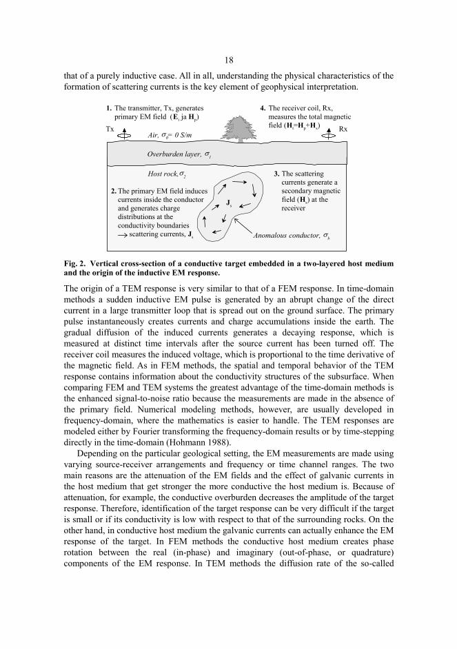
To provide an additional example, Fig. 3 shows a comparison between the half-plane solution (Appendix) and the EMPLATES method for the HCPL (horizontal co-planar loops, or Slingram) system. To model the purely inductive response, the loop spacing was 100 m, the frequency was 10000 Hz, the host resistivity was 106 Ωm, and the resistivity of the plate was 0.001 Ωm in the EMPLATES computations. In addition, the plate size

24

was 500×500 m, the discretization was 20×20, and the nominal thickness of the plate model was one meter. Fig. 3 displays the fits for different values of depth of burial (a) and dip angle (b). Fig. 3 shows a good agreement between the revised method and the half-plane solution. The example demonstrates that the approximate method can model also the inductive current mode in highly resistive surroundings.

Fig. 3. Comparison of the half-plane solution (symbols) and EMPLATES method (lines). The inductive limit response (in-phase component only) is computed for a HCPL system and different values of depth of burial (a) and dip angle (b).

On the whole, the approximate modeling method is capable of describing the characteristic behavior of the EM response of a thin plate model in conductive and resistive surroundings. Because the computational method is relatively fast, the linearized least-squares inversion method can be used to optimize the thin plate parameters efficiently. The EMPLATES software described in Paper II was developed for practical interpretation of frequency-domain EM measurements. The program can be used to model the common vertical and horizontal magnetic dipole-dipole (VMD and HMD) measurement systems, as well as the Finnish Gefinex 400S (Soininen & Jokinen 1991) and the French BRGM Melis (Valla 1991) frequency sounding systems that measure the ratio of vertical and horizontal (radial) magnetic fields. Both in-line and broadside configurations can be used, and the source and the receiver can be located at different levels above the earth's surface. Therefore, also airborne EM measurement systems can be modeled. The program can simultaneously use 5 plate models, 5 profiles, and 10 frequencies. The interaction between multiple plate models is taken into consideration in an approximate way.

The computational parts of the EMPLATES software are written in Fortran-77 language but use some Fortran-90 extensions for dynamic memory allocation, for example. The graphical user interface for the 32-bit Microsoft Windows™ 95 and above operating systems is written in C++ language. The EMPL2 and INVEMPL programs discussed in Paper IV enable the modeling and interpretation of time-domain EM

! " #

! #

! $ #

! % #

& '

25

responses. These two programs lack a graphical user interface but provide more detailed computational results than the EMPLATES program.

Algorithm 2. The EMPLATES modeling method.

1. Determine the x, y, and z coordinates of the collocation points 2. Do loop for each frequency 2.1 Read in or compute new Hankel transform values 2.2 Construct the impedance matrix, Z 2.3 Perform the LU decomposition of the impedance matrix 3. Do loop for each measurement profile 4. Do loop for each measurement point 4.1 Determine the locations of source and receiver 4.2 Compute the primary magnetic field, H0 and Hp 4.3 Derive Green's functions for the inducing electric field 4.4 Compute the primary electric field at collocation points, Ei 4.5 Solve the scattering currents using the LU decomposition, Js=Z-1 Ei 4.6 Derive Green's functions for the secondary magnetic field 4.7 Compute the secondary magnetic field, Hs 4.8 Define and store the EM response end do end do end do

A general description of the algorithm used in the EMPLATES program is presented above. The algorithm assumes an inductive dipole-dipole measurement system, where the EM response is based on the magnetic field components, and the same frequencies are used on all measurement profiles. The algorithm utilizes a 2-D interpolation of pre-computed Hankel transforms (phase 2.1) to compute the kernel functions associated with the equations of the primary inducing electric field at the collocation points (phase 4.3) and the secondary magnetic field at the receiver (phase 4.6). This method is used to reduce the amount of direct computations of time-consuming Hankel transforms. The algorithm has not been optimized to any specific measurement system. Phase 4.2, for example, needs to be made only once if fixed loop spacing is used. Likewise, phases 4.3 to 4.5 need to be performed only once if a measurement system with a fixed source position is used. The definition of the EM response at phase 4.8 depends on the particular measurement system. In the VMD-VMD system, for example, the EM response is usually the vertical total magnetic field normalized by the free-space component ((Hzp+ Hzs)/Hz0-1).

4 Analysis of the inversion characteristics

The inversion characteristics, such as the resolution, sensitivity, and correlation behavior of the thin plate parameters, have been investigated in this thesis using the misfit function (MF) mapping and the SVD analysis. The MF map is a simple 2-D visual representation, a slice, of the N-dimensional parameter space. MF mapping provides information on the uniqueness and the accuracy of the solution, and it can reveal correlation and non-linear relationships between the model parameters. As the number of model parameters increases, the analysis of the SVD information derived from the least-squares inversion provides a more economical way to study the inversion characteristics than the MF mapping. Together, the singular values and the parameter and data eigenvectors of the SVD, provide information about the sensitivity and the resolution of the model parameters. SVD analysis can also reveal more complicated correlation behavior than misfit function mapping. The information provided by the analysis methods can be used, for example, to select better initial model parameters, to guide the inversion process, and to estimate the validity of the inverse solution. They can also be used to analyze the resolving capabilities of different measurement systems. Because the results of the SVD analyses and the misfit function mapping studies depend strongly on the model and system parameters, comprehensive analysis of different models and measurement systems is beyond the scope of this thesis. The main objective is to describe useful methods to obtain valuable information for interpretation purposes.

Because the SVD analysis has been described extensively in Papers I, III, and IV, it is not discussed here further. The few MF mapping examples in Papers I and III, however, consider the TEM response of a thin plate in free-space and the FEM response of the half-plane model. Because the new approximate modeling method presented in Papers II and IV enables the investigation of a thin plate in conductive surroundings, a short description of the misfit function mapping technique and some additional examples are provided below.

27

4.1 Misfit function mapping

The misfit function mapping means a 2-D plotting of the error function, also known as the cost or objective function, over a space of model parameters. The misfit function is the difference, for example the root-mean-square (RMS) error, between two data sets computed with different parameters. The MF map is constructed with respect to a reference model, the response of which is firstly computed. The misfit function is then systematically computed for models, where two model parameters are varied around their reference values, and finally plotted as a 2-D contour or surface plot. To be able to compare different maps with each other better they have to be normalized by the maximum error, for example. If the data weighting is made adequately, the RMS error values can be used in the contour maps directly. Although 3-D MF mapping is quite possible, the problem is how to display and understand the 3-D visualizations easily.

Considering that the horizontal position and strike direction of the target are relatively easy to resolve from multi-profile data, the depth of burial (DB) and dip angle (DA) are important especially when making a decision on an optimal location and direction for drilling. The interpreted value of the conductance (CO) is important when estimating the quality of the conductor that helps to determine the rock type or mineral content of the target in geological interpretation. Examples of misfit function maps computed for the combinations of DB, DA and CO are shown in Fig. 4 separately for FEM and TEM responses. The MF maps represent three orthogonal projections that coincide at DB= 50 m, DA= 60°, CO= 10 S. The parameters of the basic model are the same as in model M1 in Paper IV (Table 1, Figs. 6 and 7). Also the parameters of the HCPL measurement system are the same as in Paper IV (3 profiles, 7 frequencies, L= 100 m, h= 1.0 m). To be able to compare the maps better, each map has been normalized by its maximum RMS error value shown above the maps. In general, Fig. 4 exhibits similar misfit function topographies in FEM (a, b, c) and TEM (d, e, f) cases. The larger maximum RMS error values of the time-domain maps indicate steeper topography, and hence, suggest better resolving capabilities of TEM methods. The dip angle is quite insensitive (b, d, e) and shows weak correlation with the conductance (a, d). The depth of burial, and its minimum value in particular, is well defined, almost unique. Fig. 4 (b) reveals that the apparent coupling between the dip angle and depth of burial in Fig. 8 (a) in Paper IV does not imply actual correlation between these two parameters, but is a consequence of the SVD, which divides the information over several singular values and combines the dip angle with other parameters. Interestingly, Figs. 4 (a) and (d) insinuate a bi-modal solution, where the dip angle could have a local minimum on the other side of the vertical position (DA>90°). Considering the asymmetric shape of the HCPL response of a dipping plate model, the possible local minimum cannot be well defined, however.

28

Fig. 4. FEM and TEM misfit function maps (normalized RMS error) computed for the dip angle, depth of burial, and conductance of a thin plate model (model M1 in Table 1 in Paper IV). The HCPL system configuration is defined in Paper IV.

20 40 60 80 100

Dip angle (deg.)

5

10

15

20

Con

duct

ance

(S)

20 40 60 80 100

Dip angle (deg.)

20

40

60

80D

epth

of b

uria

l (m

)

20 40 60 80

Depth of burial (m)

5

10

15

20

Con

duct

ance

(S)

NormalizedRMS-error

(d) Max: 1.2530

(e) Max: 1.5989

(f) Max: 2.2380

0 0.02 0.05 0.1 0.2 0.3 0.4 0.5 0.6 0.7 0.8 0.9 1

20 40 60 80 100

Dip angle (deg.)

5

10

15

20

Con

duct

ance

(S)

(a) Max: 0.5629

20 40 60 80 100

Dip angle (deg.)

20

40

60

80

Dep

th o

f bur

ial (

m)

(b) Max: 1.0755

20 40 60 80

Depth of burial (m)

5

10

15

20

Con

duct

ance

(S)

(c) Max: 1.2155

Frequency-domain Time-domain

29

Fig. 5. FEM and TEM misfit function maps (normalized RMS error) computed for the strike length and the depth extent of a thin plate model in a conductive (RH=100 Ωm) and resistive (RH=1000 Ωm) host medium. The model parameters are otherwise the same as in model M1 in Table 1 in Paper IV. The HCPL system configuration is defined in Paper IV.

The strike length (SL) and the depth extent (DE) are of great interest in geophysical interpretation, because they are used to evaluate the size and the volume of the target, and hence, the economical value of the ore body, for example. However, the depth extent of a steeply dipping target is one of the most difficult parameters to resolve from real EM data. Fig. 5 shows FEM and TEM MF maps computed for the SL-DE pair for a thin plate in a conductive (a) and (c) and a resistive (1000 Ωm) host medium. The parameters of the dipping plate model and the HCPL measurement system are otherwise the same as in the previous example and Paper IV. The vertically elongated shape of the error surface in Fig. 5 indicates that depth extent is very difficult to resolve when the host medium is conductive (100 Ωm). This can be expected, because the more conductive the host

300 400 500 600 700

Strike length (m)

100

200

300

400

500

Dep

th e

xten

t (m

)

300 400 500 600 700

Strike length (m)

100

200

300

400

500

Dep

th e

xten

t (m

)

300 400 500 600 700

Strike length (m)

100

200

300

400

500

Dep

th e

xten

t (m

)

300 400 500 600 700

Strike length (m)

100

200

300

400

500

Dep

th e

xten

t (m

)Frequency-domain Time-domain

NormalizedRMS-error 0 0.02 0.05 0.1 0.2 0.3 0.4 0.5 0.6 0.7 0.8 0.9 1

(c) RH= 100 OhmmMax: 0.2322

(a) RH= 100 OhmmMax: 0.2069

(b) RH= 1000 OhmmMax: 0.2339

(d) RH= 1000 OhmmMax: 0.2764

30

medium is, the greater is the attenuation of the EM field. For the same reason the upper limit of the strike length is not as well defined as its lower limit. When the host is resistive, the size of the plate can be better resolved. Unlike the other maps, Fig. 5 (d) shows non-linear behavior, which is similar to the misfit function maps in Papers I and III. Because the EM data for the maps in Fig. 5 were computed using three separate measurement profiles, the curvature of the misfit topography has reduced in size indicating improved resolution of strike length. When compared to Fig. 4, the small values of the RMS error reveal that the error surface is extremely flat indicating that both parameters are very insensitive. Fig. 5 indicates that TEM methods can resolve the size of the plate better than FEM methods.

Fig. 6. FEM and TEM misfit function maps (normalized RMS error) computed for the strike length and the depth extent of a thin plate model (model M1 in Table 1 in Paper IV). Comparison is made between the low and high frequency content (FEM) and the late and early time channels (TEM). The HCPL system configuration is defined in Paper IV.

300 400 500 600 700

Strike length (m)

100

200

300

400

500D

epth

ext

ent (

m)

300 400 500 600 700

Strike length (m)

100

200

300

400

500

Dep

th e

xten

t (m

)

300 400 500 600 700

Strike length (m)

100

200

300

400

500

Dep

th e

xten

t (m

)

300 400 500 600 700

Strike length (m)

100

200

300

400

500

Dep

th e

xten

t (m

)

Frequency-domain Time-domain

NormalizedRMS-error 0 0.02 0.05 0.1 0.2 0.3 0.4 0.5 0.6 0.7 0.8 0.9 1

(c) Late timesMax: 0.4238

(a) Low frequenciesMax: 0.2227

(b) High frequenciesMax: 0.2116

(d) Early timesMax: 0.2354

31

Fig. 6 shows an example of the misfit function mapping, where the strike length and depth extent are mapped using the three lowest and the three highest frequencies of FEM data and the three latest and the three earliest time channels of TEM data. The system and model parameters are the same as in the previous examples and model M1 in Paper IV. Fig. 6 confirms that the low frequencies and the late time channels define the true solution better than the high frequency and the early time channel. However, the positions of the peak misfit reveal a certain difference between FEM and TEM methods that can be explained by the diffusion of the currents. As time passes, the currents move downward and away from the EM source. In the early time TEM misfit function map (d) the largest errors are obtained at small values of strike length, whereas at late time (c) the largest misfit is obtained when the plate is large. This indicates that early time TEM data resolves the lower limit of the strike length and late time channels are needed to resolve the maximum size of the plate model. Comparison to Fig. 5 shows that when all time channels are used together the overall resolution improves. The FEM misfit function maps, on the other hand, do not reveal as strong a relationship. Surprisingly, comparison to Fig. 5 indicates that the size of the plate is resolved better when the low frequency part of the FEM data is used alone than when all frequencies are used together. Considering the results obtained from the analysis of data eigenvectors in Paper IV, this confirms that the high frequency FEM data can disturb the resolution of the least sensitive parameters. The results suggest that in frequency-domain the interpretation of plate size should be based on low frequency data alone.

Besides the ease of visual inspection, the greatest advantage of misfit function mapping is its ability to display large-scale non-linear relationships between the model parameters. The SVD information is obtained from a single point in the parameter space. These techniques should preferably be used together, so that the MF mapping provides a general view and the SVD analysis gives more detailed information about a particular solution. Unfortunately, complete MF mapping is an exhaustive computational task especially in the TEM case. Considering that several maps are needed to display even the most interesting 2-D projections of an N-dimensional parameter space, comprehensive MF mapping is impractical for the TEM systems. In the FEM interpretations, however, MF mapping could be used to assess the accuracy of the inverse solution if the misfit is mapped with respect to real data. An important thing to remember when considering the utilization of MF mapping, is that the 2-D MF maps are approximate representations of the variability of model parameters, because the remaining parameters are held fixed at their true values. The real variability of various parameters is always greater than or equal to that shown by the MF maps (L.B. Pedersen, pers. comm.).

5 Discussion and conclusions

The main objectives of this study were to study the EM induction phenomenon and to develop practical interpretation tools for geophysical EM measurements. The thin plate model was used, because of its simplicity and suitability for various geological problems. Moreover, the EM response of a thin plate can be modeled with the integral equation method, which does not require as vast computational resources as full 3-D modeling with differential equations. Similarly, the linearized least-squares inversion method was used because it allows efficient optimization and the thin plate model has only a few parameters. Furthermore, the visual inspection of EM profile data provides good initial values for several model parameters. The adaptive damping method provides stable and fast convergence and avoids unnecessary forward computations. Because the linearized inversion is a local optimization method, it is used in this study more as an additional tool for the interpreter than as a full-scale inversion method. The lattice model formulation was employed in the formulation of the forward problem, because it enables the modeling of both the inductive and galvanic current modes. Additional approximations were made to improve the computational speed and to provide a stable solution. The original computational method was developed for frequency-domain EM methods. Time-domain EM responses are modeled using a Fourier-sine transform of broadband frequency-domain responses.

Both the model and the approximations used in the computational method impose restrictions on the general applicability of the modeling method. The critical factor is the thin plate model itself. Although it can be used to represent several types of geological structures it is still a very limited model. In the real world, the true conductivity structures are more complicated than what can be modeled with thin, rigid, rectangular plate models. Furthermore, the conductive target and the host medium are likely to have non-homogenous conductivity, and both the thickness and the conductivity of the overburden layer (or layers) have spatial variations below the survey area. This so-called geological noise is often a more severe factor affecting the interpretation than the noise arising from the instrumentation, alignment errors, or cultural sources, for example. If the geological noise is sufficiently large, the difference between the measured and the modeled EM responses will cause incorrect results in the inversion. In the worst case, a thin conductor in two-layered host medium is a totally inappropriate representation of the true

33

conductivity structure. Quantitative interpretation of EM data becomes then possible only if a more appropriate 3-D modeling method is used. In this case, however, the computation requirements can become prohibitive in practice.

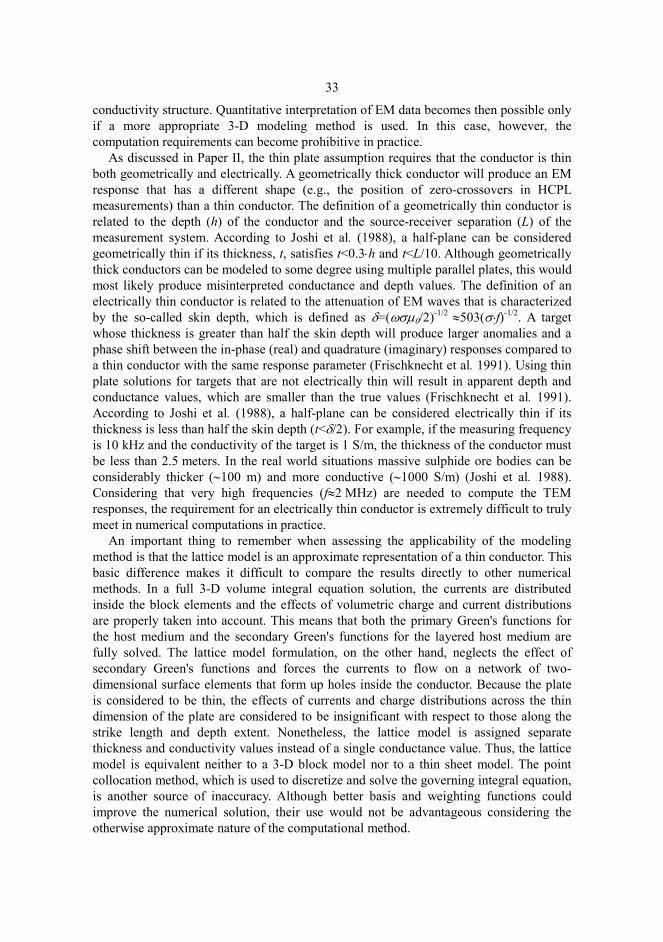
As discussed in Paper II, the thin plate assumption requires that the conductor is thin both geometrically and electrically. A geometrically thick conductor will produce an EM response that has a different shape (e.g., the position of zero-crossovers in HCPL measurements) than a thin conductor. The definition of a geometrically thin conductor is related to the depth (h) of the conductor and the source-receiver separation (L) of the measurement system. According to Joshi et al. (1988), a half-plane can be considered geometrically thin if its thickness, t, satisfies t<0.3⋅h and t<L/10. Although geometrically thick conductors can be modeled to some degree using multiple parallel plates, this would most likely produce misinterpreted conductance and depth values. The definition of an electrically thin conductor is related to the attenuation of EM waves that is characterized by the so-called skin depth, which is defined as δ=(ωσµ0/2)-1/2 ≈503(σ⋅f)-1/2. A target whose thickness is greater than half the skin depth will produce larger anomalies and a phase shift between the in-phase (real) and quadrature (imaginary) responses compared to a thin conductor with the same response parameter (Frischknecht et al. 1991). Using thin plate solutions for targets that are not electrically thin will result in apparent depth and conductance values, which are smaller than the true values (Frischknecht et al. 1991). According to Joshi et al. (1988), a half-plane can be considered electrically thin if its thickness is less than half the skin depth (t<δ/2). For example, if the measuring frequency is 10 kHz and the conductivity of the target is 1 S/m, the thickness of the conductor must be less than 2.5 meters. In the real world situations massive sulphide ore bodies can be considerably thicker (∼100 m) and more conductive (∼1000 S/m) (Joshi et al. 1988). Considering that very high frequencies (f≈2 MHz) are needed to compute the TEM responses, the requirement for an electrically thin conductor is extremely difficult to truly meet in numerical computations in practice.

An important thing to remember when assessing the applicability of the modeling method is that the lattice model is an approximate representation of a thin conductor. This basic difference makes it difficult to compare the results directly to other numerical methods. In a full 3-D volume integral equation solution, the currents are distributed inside the block elements and the effects of volumetric charge and current distributions are properly taken into account. This means that both the primary Green's functions for the host medium and the secondary Green's functions for the layered host medium are fully solved. The lattice model formulation, on the other hand, neglects the effect of secondary Green's functions and forces the currents to flow on a network of two-dimensional surface elements that form up holes inside the conductor. Because the plate is considered to be thin, the effects of currents and charge distributions across the thin dimension of the plate are considered to be insignificant with respect to those along the strike length and depth extent. Nonetheless, the lattice model is assigned separate thickness and conductivity values instead of a single conductance value. Thus, the lattice model is equivalent neither to a 3-D block model nor to a thin sheet model. The point collocation method, which is used to discretize and solve the governing integral equation, is another source of inaccuracy. Although better basis and weighting functions could improve the numerical solution, their use would not be advantageous considering the otherwise approximate nature of the computational method.

34

The biggest problem is the lack of a theoretical solution for the scaling factor, or an equivalent functional, which would properly define the total electric field for the discrete lattice elements. Instead, modeling comparisons to other numerical methods and the conductance criterion have been used to determine the necessary adjustments for the diagonal elements of the impedance matrix. The corrections that were made in Paper IV do not fully satisfy the conductance criterion, and therefore, the plate thickness should be fixed to one meter in numerical computations in practice. However, the revisions improve particularly the low frequency part of the EM response, and hence, the accuracy of interpreted depth values so that the depth compensation method used in Paper II has become more or less obsolete. The depth compensation method, which is modified according to the revised scaling factor, could still be useful when the host is highly resistive and the target has low conductance. It is noteworthy that the corrections made to the revised modeling method are mostly quantitative, and therefore, they do not diminish the general reliability of the results of Paper II.

The results presented in this study demonstrate that the approximate computational method can model the geophysical frequency and time-domain EM responses of a thin conductor in conductive host medium with sufficient accuracy, and that the inversion method can provide reliable estimates for the model parameters. Considering the overall ambiguity involved with the interpretation of real EM data, the limitations of the modeling method are not critical.

The main advantages of the approximate modeling method are summarized in the following.

1. The thin plate model suits to many geological situations:

a) The effect of conductive host and overburden can be modeled,

b) Large conductivity contrast situation can be tolerated,

c) The interaction between multiple conductors can be modeled,

d) The orientation and position of the plates can be almost arbitrary, and

e) Complex structures can be modeled with multiple plate models.

2. Several EM measurement systems can be modeled:

a) FEM and TEM measurement systems,

b) HMD and VMD source systems (including airborne EM systems),

c) Fixed loop spacing and fixed loop position systems, and

d) In-line and broadside configurations.

3. The computation is relatively fast:

a) The method suits to microcomputer environment,

b) Interactive inversion of FEM data is possible, and

c) Feasible forward modeling of TEM data is possible.

35

Besides its use in practical interpretation, the modeling method gives a possibility to study the forward and the inverse problem of the EM induction phenomenon. Because of the simplicity of the model the method is particularly well suited for educational purposes.

When considering the various analysis results presented in this thesis and the performance of the inversion methods in general, the use of data weighting or scaling is of great importance. If scaling is not used at all, the inversion will emphasize those response components that have the largest amplitudes. In practice, this means that the inverse solution will be based mainly on the high frequency part of the FEM response or the early time data of the TEM response. Consequently, the resolution of the plate size and conductance will reduce, because their interpretation needs the information from the low frequency or late time response as indicated by the data eigenvectors in Fig. 10 in Paper IV, for example. The scaling defined by Eq. (2) in Paper IV normalizes each data channel with the peak-to-peak difference of the measured data. Considering that some kind of scaling is necessary in practice, the one used here is practical when making a comparative study and working with synthetic data, because it gives equal weight to all data channels. It is noteworthy that the scaling method does not pass the noise of individual data values into the SVD results.

However, equal weighting can be unsafe when interpreting real field data that contains errors. Because of the attenuation of EM fields, for example, the signal-to-noise ratio decreases when the measurement frequency of FEM data decreases or the time channel of TEM data increases. For the same reason, the geological noise affects different measurement points, frequencies and time channels differently. The various data components (e.g., vertical and horizontal fields) and the response components of FEM data (in-phase and quadrature) are sensitive to the noise in different ways as well. Additional weighting that is based on the estimated data errors should therefore be applied in practice to suppress the effect of erroneous or noisy data values and data channels. In this thesis, where synthetic data has mainly been used, additional weighting has not been used.

Because the frequency-domain and the time-domain data are related through a Fourier-transform, they contain theoretically the same information provided that the data are measured over an infinite frequency or time range using an infinitesimal sampling. Therefore, they should reveal the same inversion characteristics as well. The analysis results of this study, however, indicate that time-domain methods have slightly better interpretation capabilities than frequency-domain methods. The two main reasons for the differences are the limited bandwidth and the finite sampling of frequencies and time channels. The data scaling treats the FEM and TEM data slightly differently as well. A more detailed study of the various effects of noise, data sampling, scaling and weighting would be needed to analyze the true resolution of the parameters of thin plate model in the inversion of FEM and TEM data.

References

Anderson WL (1984) Fast Hankel transforms using related and lagged convolutions. ACM Trans. on Math. Software 8: 344-368.

Annan AP (1974) The equivalent source method for electromagnetic scattering analysis and its geophysical application. PhD thesis, Memorial Univ. of Newfoundland.

Chen, J, Raiche, A & Macnae, J (2000) Inversion of airborne EM data using thin-plate models. 70th Ann. Mtg: Soc. of Expl. Geophys., Expanded Abstracts: 355-358.

Christensen NB (1990) Optimized fast Hankel transform filters. Geoph. Prospecting 38: 545-568. Christensen NB (1997) Electromagnetic subsurface imaging - a case for an adaptive Born

approximation. Surv. in Geophysics 18: 477-510. Coggon JH (1971) Electromagnetic and electrical modeling by the finite element method.

Geophysics 36: 132-155. Frischknecht FC, Labson VF, Spies BR & Anderson WL (1991) Profiling methods using small

sources. In: Nabighian MN (ed) Electromagnetic methods in applied geophysics, Volume 2, Applications. Soc. of Expl. Geophys., Tulsa, p. 105-270.

Grant FS & West GF (1965) Interpretation theory in applied geophysics. McGraw-Hill, New York. Hohmann GW (1971) Electromagnetic scattering by conductors in the earth near a line source of

current. Geophysics 36: 101-131. Hohmann GW (1975) Three-dimensional induced polarization and electromagnetic modeling.

Geophysics 40: 309-324. Hohmann GW (1988) Numerical modeling for electromagnetic methods of geophysics. In:

Nabighian MN (ed) Electromagnetic methods in applied geophysics, Volume 1, Theory. Soc. of Expl. Geophys., Tulsa, p. 313-363.

Hohmann GW & Raiche AP (1988) Inversion of controlled-source electromagnetic data. In: Nabighian MN (ed) Electromagnetic methods in applied geophysics, Volume 1, Theory. Soc. of Expl. Geophys., Tulsa, p. 469-503.

IMSL (1994) IMSL MATH/LIBRARY User's Manual, Version 3.0. IMSL, Houston. Joshi MS, Gupta OP & Negi JG (1988) On the effects of thickness of the half-plane model in

HLEM induction prospecting over sulphide dykes in a highly resistive medium. Geoph. Prospecting 36: 551-558.

Jupp DLB & Vozoff K (1975) Stable iterative methods for the inversion of geophysical data. Geophys. J. R. Astr. Soc. 42: 957-976.

37

Kwan KCH & Edwards RN (1988) A novel method of computing the EM response of a conducting plate in conductive host. 58th Ann. Mtg, Soc. of Expl. Geophys., Anaheim, California, Expanded Abstracts: 222-225.

Kwan KCH (1989) A novel method of computing the EM response of a conducting plate in conductive medium. Res. in Appl. Geoph. N:o 45, Dept. of Physics, Univ. of Toronto.

Lee KH, Pridmore DF & Morrison HF (1981) A hybrid three-dimensional electromagnetic modeling scheme. Geophysics 46: 796-805.

Lee KH, Liu G & Morrison HF (1989) A new approach to modeling the electromagnetic response of conductive media. Geophysics 54: 1180-1192.

Lines LR (ed) (1988) Inversion of geophysical data. Geophysics Reprints No. 9: Soc. Expl. Geophys., Tulsa.

Liu EH & Lamontage Y (1998) Geophysical application of a new surface integral equation method for EM modeling. Geophysics 63: 411-423.

Mackie RL, Madden TR & Wannamaker PE (1993) Three-dimensional magneto-telluric modeling using difference equations. Geophysics 58: 215-226.

Marquardt DW (1963) An algorithm for least-squares estimation of non-linear parameters. J. SIAM 11: 431-441.

Mitsuhata Y (2000) 2-D electromagnetic modeling by finite-element method with a dipole source and topography. Geophysics 65: 465-475.

Nabighian MN (1970) Quasi-static transient response of a conducting sphere in a dipolar field. Geophysics 35: 303-309.

Nabighian MN (1979) Quasi-statictransient response of a conducting half-space − An approximate representation. Geophysics 44: 1700-1705.

Nabighian MN & Macnae JC (1991) Time domain electromagnetic prospecting methods. In: Nabighian MN (ed) Electromagnetic methods in applied geophysics, Volume 2, Applications. Soc. of Expl. Geophys., Tulsa, p. 427-520.

Newman GA, Hohmann GW & Anderson WL (1986) Transient electromagnetic response of a three-dimensional body in a layered earth. Geophysics 51: 1608-1627.

Newman GA & Hohmann GW (1988) Transient electromagnetic responses of high-contrast prisms in a layered earth. Geophysics 53: 691-706.

Oristaglio M & Spies R (1999) Three-dimensional electromagnetics. Soc. of Expl. Geophys., Tulsa. Parry J R (1969) Integral equation formulations of scattering from two-dimensional

inhomogeneities in a conductive earth. PhD thesis, Berkeley, University of California. Press WH, Flannery BP, Teukolsky SA & Vetterling WT (1988) Numerical recipes in Fortran 77,

the art of scientific computing. Cambridge Univ. Press. Raiche AP (1974) An integral equation approach to 3D modeling. Geophys. J. R. Astr. Soc. 36:

363-376. Raiche AP (1994) Modelling and inversion - progress, problems, and challenges. Surv. in

Geophysics 15: 159-207. Sasaki K (2001) Full 3-D inversion of electromagnetic data on PC. J. Appl. Geophysics 46: 45-54. Sen MK & Stoffa PL (1995) Global optimization methods in geophysical inversion. Elsevier

Science, Amsterdam. Soininen H & Jokinen T (1991) Sampo, a new wide-band electromagnetic system. 53rd EAEG

meeting and technical exhibition, Florence, Italy, Technical programme and abstracts of papers: 366-367.

38

Spies BR & Frischknecht FC (1991) Electromagnetic sounding. In: Nabighian MN (ed) Electromagnetic methods in applied geophysics, Volume 2, Applications. Soc. of Expl. Geophys., Tulsa, p. 285-425.

Torres-Verdín C & Habashy TM (1994) Rapid 2.5-dimensional forward modeling and inversion via a new nonlinear scattering approximation. Radio Science 29: 1051-1079.

Valla P (1991) BRGM Melis multifrequency EM system. In: Nabighian MN (ed) Electromagnetic methods in applied geophysics, Volume 2, Applications. Soc. of Expl. Geophys., Tulsa, pp. 417-421.

Wang T & Hohmann GW (1993) A finite-difference time-domain solution for three-dimensional electromagnetic modeling. Geophysics 58: 797-809.

Wannamaker PE, Hohmann GW & SanFilipo WA (1984) Electromagnetic modeling of three-dimensional bodies in layered earths using integral equations. Geophysics 49: 60-74.

Ward SH (1980) Electrical, electromagnetic, and magnetotelluric methods. Geophysics 45: 1659-1666.

Ward SH & Hohmann GW (1988) Electromagnetic theory for geophysical applications. In: Nabighian MN (ed) Electromagnetic methods in applied geophysics, Volume 1, Theory. Soc. of Expl. Geophys., Tulsa, p. 131-311.

Weidelt P (1975) Electromagnetic induction in three-dimensional structures. J. Geophys. 41: 85-109.

Weidelt, P (1981) Dipolinduktion in einer dünnen Platte mit leitfähiger Umgebung und Deckschicht. Report 89727, BGR, Hannover.

West GF & Macnae JC (1988) Physics of the electromagnetic induction exploration method. In: Nabighian MN (ed) Electromagnetic methods in applied geophysics, Volume 1, Theory. Soc. of Expl. Geophys., Tulsa, p. 427-520.

Xiong Z (1992) Electromagnetic modeling of three-dimensional structures by the method of system iteration using integral equations. Geophysics 57: 1556-1561.

Zhdanov MS & Fang S (1996) Quasi-linear approximation in 3-D electromagnetic modeling. Geophysics 61: 646-665.

Appendix

A Fortran-90 subroutine that computes the secondary magnetic field generated by an arbitrarily oriented magnetic dipole in the vicinity of a perfectly conducting half-plane in free-space is included below. The subroutine is based on the solution defined in Grant and West (1965). The algorithm is used in the HPLANE modeling program, which is freely available at <http://www.gf.oulu.fi/~mpi/>. !----------------------------------------------------------------- ! Description: ! ! This subroutine computes the EM response of a perfectly ! conducting half-plane in free-space for any dipole-dipole ! measurement system. ! ! Author: ! ! Markku Pirttijarvi, 2001-2003 ! University of Oulu, Department of Geophysics ! E-mail: markku.pirttijarvi@oulu.fi ! ! Reference: ! ! F.S. Grant & G.F West, 1965: Interpretation theory in applied ! geophysics. McGraw-Hill, New York. p. 520-528. ! ! Input: ! ! p real, dim=4, xyz position and angle of the source: x,y,z,fii ! p1 real, dim=4, xyz pos. and angle of the receiver: x,y,z,fii ! m real, dim=3, xyz components of the dipole moment : mx,my,mz ! ! Output: ! ! h real, dim=3, components of the sec. magnetic field: hx,hy,hz ! ! Notes: ! ! - All I/O parameters are defined in a local xyz coordinate

! system. ! ! - The local coordinate system is defined by the half-plane, ! which is located at the yz plane (x=0) so that the "top" edge ! of the half-plane coincides with the origin. Thus, the half- ! plane extends from y= -infinity to y= +infinity and z= 0 to ! z= -infinity. ! - Before calling this subroutine, the true xyz coordinates of ! the source and the receiver, as well as the directions of the ! source moment must be rotated to the local coordinate system ! ! - Likewise, after this subroutine the secondary magnetic field ! must be rotated from the local coordinate system to the true ! coordinate system. ! ! - The angles p(4) to the source and p1(4) to the receiver are ! taken in the local coordinate system in counter-clockwise ! orientation from the positive x axis (horiz. plane). For ! example, fii= -180° if x= -infinity, and fii= 0° if ! x= +infinity). !----------------------------------------------------------------- subroutine hplane(p,p1,m,h) implicit none integer :: i real :: mr,mf,r1,r2,ro,ro1,df,cf,sf,ca,sa,cc,ss,sr2,g1,g2,srp real :: gg1,gg2,xx,yy,zz,ax,ay,az,bx,by,bz,cr,ccf,dx,dy,dz real :: er,ef,fr,ff,pii,pii2,pii4,a1,rg2,a2,rpg,gpr,gpr2 real :: ata,eps,p14,p11,m1,u1(2,3),u2(2,2) real, dimension(4) :: p,p1 real, dimension(3) :: m,h pii= 4.*atan(1.) pii2= pii*pii pii4= 4.*pii2 cc= cos(p(4)) ss= sin(p(4)) ! loop for source and image terms do i=1,2 if (i == 1) then p14= p1(4) p11= p1(1) m1= m(1) else p14= pii-p1(4) p11= -p1(1) m1= -m(1) end if

df= (p14-p(4))/2. cf= cos(df) sf= sin(df) ca= cos(p14) sa= sin(p14) xx= p11-p(1) yy= p1(2)-p(2) zz= p1(3)-p(3) r1= sqrt(xx*xx+yy*yy+zz*zz) ! handle singularity by a small shift: image is at receiver point if (i == 1) then eps=r1/100. end if if (r1 < eps) r1=eps r2= r1*r1 ro= sqrt(p(1)*p(1)+p(2)*p(2)) ro1= sqrt(p11*p11+p1(2)*p1(2)) sr2= 2.*sqrt(ro*ro1) g1= sr2*cf g2= g1*g1 mr= ca*m1+sa*m(2) mf= ca*m(2)-sa*m1 srp= sqrt(ro/ro1) gg1= (m1*xx+m(2)*yy+m(3)*zz)/r1 gg2= (mr*cf-mf*sf)*srp ax= -xx*gg1/r1 ay= -yy*gg1/r1 az= -zz*gg1/r1 bx= (xx*gg1-m1*r1)/r2 by= (yy*gg1-m(2)*r1)/r2 bz= (zz*gg1-m(3)*r1)/r2 cr= (mr*cf-mf*sf)/sr2 ccf= (mr*sf+mf*cf)/sr2 dx= -xx*gg2/r1 dy= -yy*gg2/r1 dz= -zz*gg2/r1 er= cf*gg1/srp ef= sf*gg1/srp fr= cf*gg2/srp ff= sf*gg2/srp a1= 1./(pii4*r2) rg2= (r2+g2) a2= 1./(pii4*rg2) rg2= 2./rg2 gpr= g1/r1 gpr2= gpr*gpr ata= atan2(r1,g1)

u1(i,1)= a1*(2*ax/r1-bx)*ata u1(i,1)= a2*(gpr*bx+rg2*(r1*dx-g1*ax*(2.+gpr2)))+u1(i,1) u1(i,2)= a1*(2*ay/r1-by)*ata u1(i,2)= a2*(gpr*by+rg2*(r1*dy-g1*ay*(2.+gpr2)))+u1(i,2) u1(i,3)= a1*(2*az/r1-bz)*ata u1(i,3)= a2*(gpr*bz+rg2*(r1*dz-g1*az*(2.+gpr2)))+u1(i,3) u2(i,1)= a2*(-cr+rg2*(r1*er+g1*fr)) u2(i,2)= a2*(-ccf+rg2*(r1*ef+g1*ff)) u1(i,1)= u1(i,1)+u2(i,1)*cc-u2(i,2)*ss u1(i,2)= u1(i,2)+u2(i,2)*cc+u2(i,1)*ss end do ! combine source and image parts h(1)= u1(1,1)-u1(2,1) h(2)= u1(1,2)-u1(2,2) h(3)= u1(1,3)-u1(2,3) return end subroutine hplane