3A: THE OSCILLOSCOPE Introduction - IU B · PDF file3A: THE OSCILLOSCOPE ... important component of the oscilloscope is the cathode ray tube ... and tell you how to get the oscilloscope

Acoustic Lab#3A Oscilloscope - 1 -

3A: THE OSCILLOSCOPE

Introduction The oscilloscope is a universal measuring instrument with applications in physics, biology, chemistry, medicine, and many other scientific and technological areas. It is used to give a visual representation of electrical voltages. Thus, any quantity which can be converted to a voltage can be displayed on an oscilloscope. Although the oscilloscope looks very complicated, once you familiarize yourself with its controls and functions, it is surprisingly easy to use.

The purpose of this experiment is to develop familiarity with the oscilloscope and with the types of measurements that can be made with it.

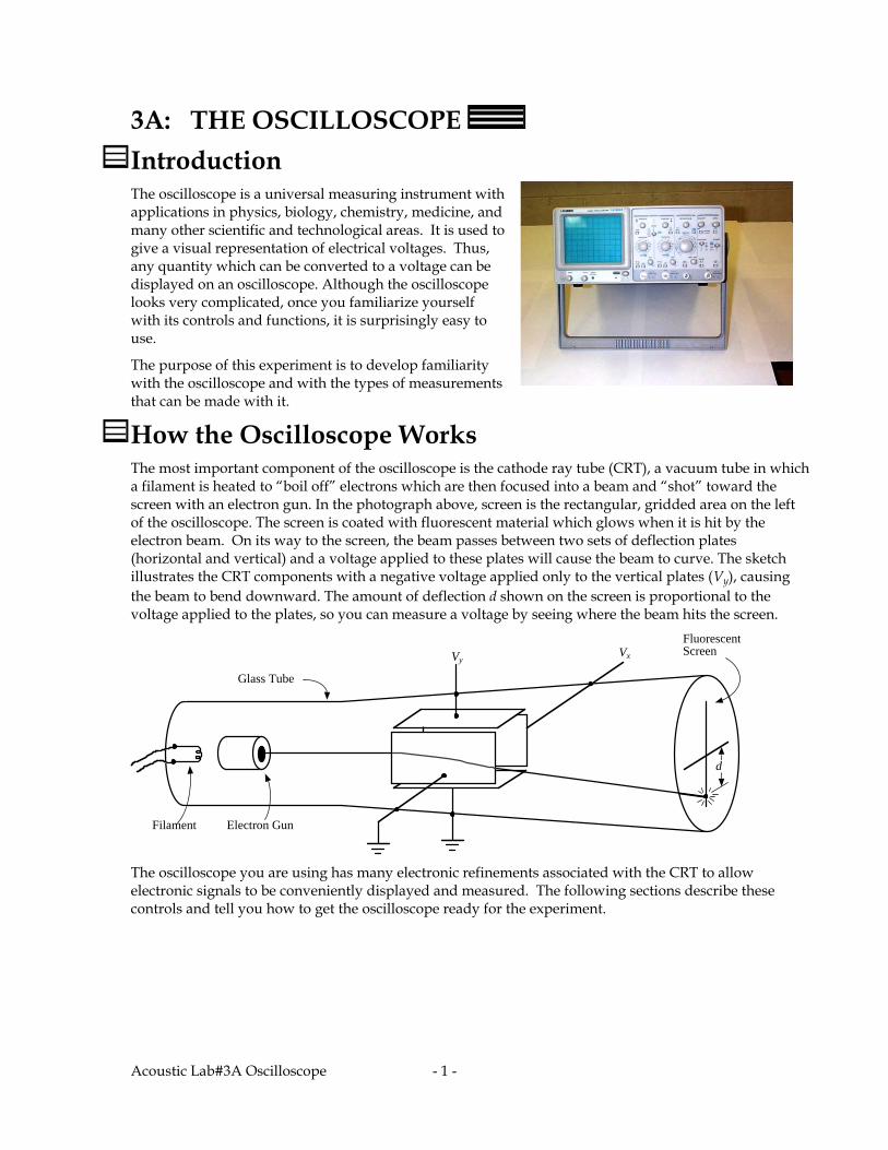
How the Oscilloscope Works The most important component of the oscilloscope is the cathode ray tube (CRT), a vacuum tube in which a filament is heated to “boil off” electrons which are then focused into a beam and “shot” toward the screen with an electron gun. In the photograph above, screen is the rectangular, gridded area on the left of the oscilloscope. The screen is coated with fluorescent material which glows when it is hit by the electron beam. On its way to the screen, the beam passes between two sets of deflection plates (horizontal and vertical) and a voltage applied to these plates will cause the beam to curve. The sketch illustrates the CRT components with a negative voltage applied only to the vertical plates (Vy), causing the beam to bend downward. The amount of deflection d shown on the screen is proportional to the voltage applied to the plates, so you can measure a voltage by seeing where the beam hits the screen.

The oscilloscope you are using has many electronic refinements associated with the CRT to allow electronic signals to be conveniently displayed and measured. The following sections describe these controls and tell you how to get the oscilloscope ready for the experiment.

Glass Tube

FluorescentScreen

Electron GunFilament

d

VyVx


Getting Started Look at all those knobs! Looks complicated, doesn't it? Relax. Prepare to enjoy this. We tell you step by step how to work the scope and the function generator. It really isn't as bad as it looks. As you work through this experiment, feel free to twiddle the knobs as much as you want. As long as you don't wrench them off their shafts, there are NO control settings that will harm the equipment or endanger you.

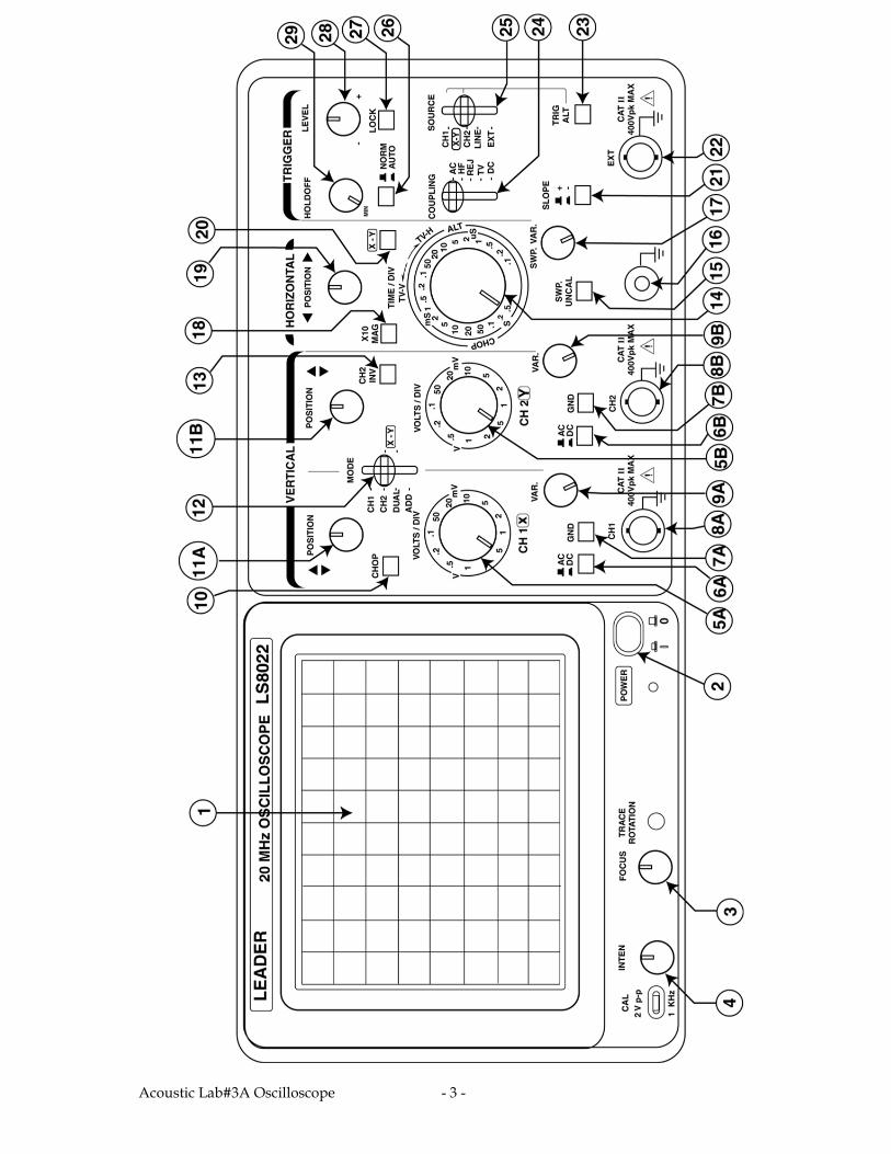
On the next page is a drawing of the scope with the controls labeled using circled numbers. As much as possible, controls have been paired. For example, numbers 5A, 6A, 7A etc. control the same functions for channel 1 (CH1) as numbers 5B, 6B, 7B etc. control for channel 2 (CH2).

Note that the scope is divided into four major areas, the SCREEN area on the left, the VERTICAL section, in the middle, the Horizontal section and the TRIGGER section on the right. We will look what the controls for each of these sections do, one at a time. Don’t worry if you can’t remember everything. The oscilloscope is surprisingly intuitive in its operation. Once you have used the scope a few times its operation becomes almost automatic.

By this time you should be practically bored to death so let’s do something! First, let’s turn on the scope and observe some electrical signals.

• Push in the POWER button (2) and push in the X-Y switch located in the HORIZONTAL section.

• Turn all three POSITION controls (11A, 11B and 19), to 12 o’clock (mark up, like so: ). Turn the INTENSITY control up until a dot appears on the screen. If no dot appears, ask your instructor for help.

• Play with the FOCUS(3) and INTENSITY (4) controls . Use the focus knob to get a sharp round dot. Use only as much intensity as you need; excessive brightness for prolonged periods can damage the screen.

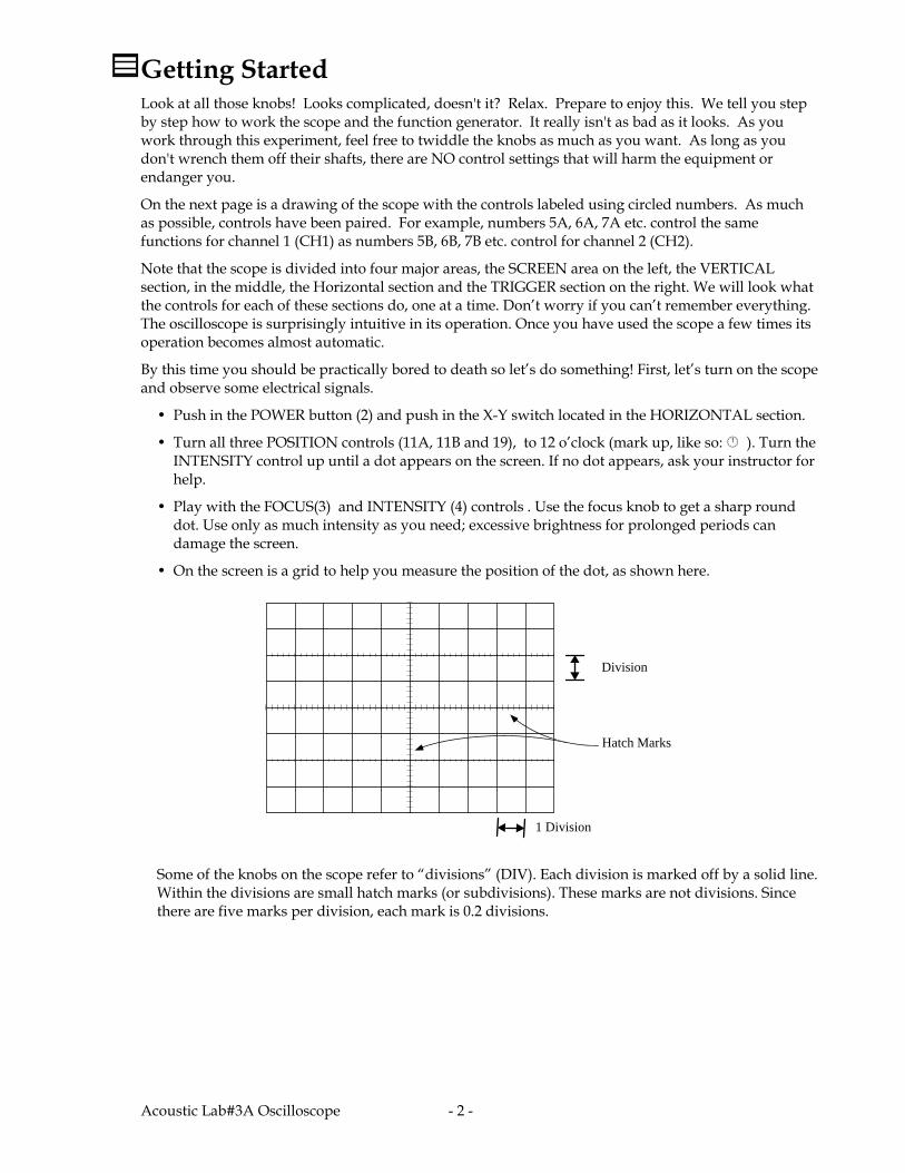
• On the screen is a grid to help you measure the position of the dot, as shown here.

Some of the knobs on the scope refer to “divisions” (DIV). Each division is marked off by a solid line. Within the divisions are small hatch marks (or subdivisions). These marks are not divisions. Since there are five marks per division, each mark is 0.2 divisions.

1 Division

1 Division

Hatch Marks



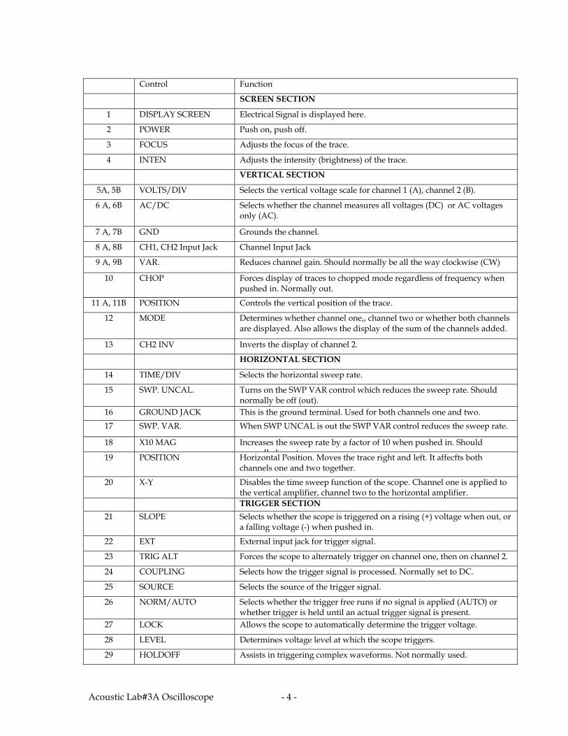
Control Function

SCREEN SECTION

1 DISPLAY SCREEN Electrical Signal is displayed here.

2 POWER Push on, push off.

3 FOCUS Adjusts the focus of the trace.

4 INTEN Adjusts the intensity (brightness) of the trace.

VERTICAL SECTION

5A, 5B VOLTS/DIV Selects the vertical voltage scale for channel 1 (A), channel 2 (B).

6 A, 6B AC/DC Selects whether the channel measures all voltages (DC) or AC voltages only (AC).

7 A, 7B GND Grounds the channel.

8 A, 8B CH1, CH2 Input Jack Channel Input Jack

9 A, 9B VAR. Reduces channel gain. Should normally be all the way clockwise (CW)

10 CHOP Forces display of traces to chopped mode regardless of frequency when pushed in. Normally out.

11 A, 11B POSITION Controls the vertical position of the trace.

12 MODE Determines whether channel one,, channel two or whether both channels are displayed. Also allows the display of the sum of the channels added.

13 CH2 INV Inverts the display of channel 2.

HORIZONTAL SECTION

14 TIME/DIV

Selects the horizontal sweep rate.

15 SWP. UNCAL. Turns on the SWP VAR control which reduces the sweep rate. Should normally be off (out).

16 GROUND JACK This is the ground terminal. Used for both channels one and two.

17 SWP. VAR. When SWP UNCAL is out the SWP VAR control reduces the sweep rate.

18 X10 MAG Increases the sweep rate by a factor of 10 when pushed in. Should normally be out 19 POSITION Horizontal Position. Moves the trace right and left. It affecfts both channels one and two together.

20 X-Y Disables the time sweep function of the scope. Channel one is applied to the vertical amplifier, channel two to the horizontal amplifier.

TRIGGER SECTION

21 SLOPE Selects whether the scope is triggered on a rising (+) voltage when out, or a falling voltage (-) when pushed in.

22 EXT External input jack for trigger signal.

23 TRIG ALT Forces the scope to alternately trigger on channel one, then on channel 2.

24 COUPLING Selects how the trigger signal is processed. Normally set to DC.

25 SOURCE Selects the source of the trigger signal.

26 NORM/AUTO Selects whether the trigger free runs if no signal is applied (AUTO) or whether trigger is held until an actual trigger signal is present.

27 LOCK Allows the scope to automatically determine the trigger voltage.

28 LEVEL Determines voltage level at which the scope triggers.

29 HOLDOFF Assists in triggering complex waveforms. Not normally used.



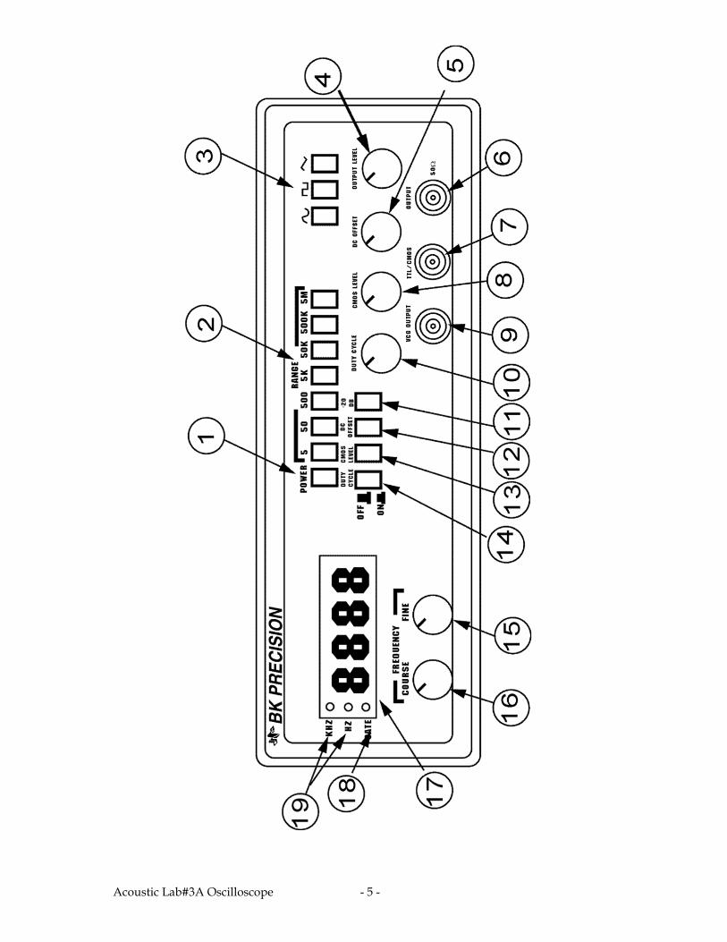
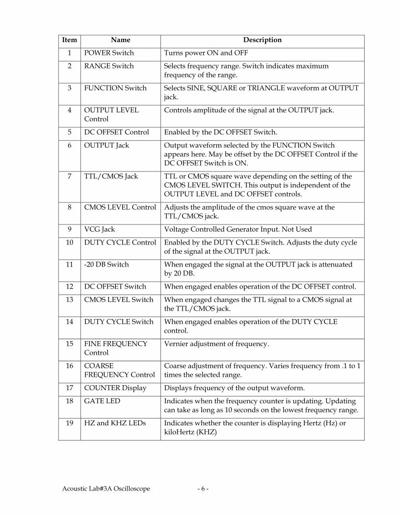
Item Name Description

1 POWER Switch Turns power ON and OFF

2 RANGE Switch Selects frequency range. Switch indicates maximum frequency of the range.

3 FUNCTION Switch Selects SINE, SQUARE or TRIANGLE waveform at OUTPUT jack.

4 OUTPUT LEVEL Control

Controls amplitude of the signal at the OUTPUT jack.

5 DC OFFSET Control Enabled by the DC OFFSET Switch.

6 OUTPUT Jack Output waveform selected by the FUNCTION Switch appears here. May be offset by the DC OFFSET Control if the DC OFFSET Switch is ON.

7 TTL/CMOS Jack TTL or CMOS square wave depending on the setting of the CMOS LEVEL SWITCH. This output is independent of the OUTPUT LEVEL and DC OFFSET controls.

8 CMOS LEVEL Control Adjusts the amplitude of the cmos square wave at the TTL/CMOS jack.

9 VCG Jack Voltage Controlled Generator Input. Not Used

10 DUTY CYCLE Control Enabled by the DUTY CYCLE Switch. Adjusts the duty cycle of the signal at the OUTPUT jack.

11 -20 DB Switch When engaged the signal at the OUTPUT jack is attenuated by 20 DB.

12 DC OFFSET Switch When engaged enables operation of the DC OFFSET control.

13 CMOS LEVEL Switch When engaged changes the TTL signal to a CMOS signal at the TTL/CMOS jack.

14 DUTY CYCLE Switch When engaged enables operation of the DUTY CYCLE control.

15 FINE FREQUENCY Control

Vernier adjustment of frequency.

16 COARSE FREQUENCY Control

Coarse adjustment of frequency. Varies frequency from .1 to 1 times the selected range.

17 COUNTER Display Displays frequency of the output waveform.

18 GATE LED Indicates when the frequency counter is updating. Updating can take as long as 10 seconds on the lowest frequency range.

19 HZ and KHZ LEDs Indicates whether the counter is displaying Hertz (Hz) or kiloHertz (KHZ)


Measuring DC Voltages The oscilloscope is fundamentally, a voltmeter. You are provided with a box which produces eight different voltages to measure. The box has already been connected to a power supply, so you can simply turn on the power supply and you are ready to go.

Defining Zero In the HORIZONTAL section, place the X-Y switch (20) in the IN position. This turns off the time base so the dot will not move horizontally across the screen.

In the VERTICAL, CH2 section, place the MODE switch (12) in the CH2 position. Then push the CH2 AC/DC coupling switch (6B) IN to DC couple the signal to the scope. Set the CH2 VOLTS/DIV switch (5B) to the 5V/DIV position. Using one of the leads provided, connect the ground terminal of the scope (16) to the black ground terminal of the voltage box, both of which are marked with the ground symbol . All voltages are measured relative to this ground. Now use another lead to connect the CH2 input (8B) to the ground. Since ground is defined to be zero, you are now measuring zero volts. Use the CH2 position control (11B) to move the dot on the screen up or down to some convenient place. Since all of the voltages you will be measuring in this section will be positive, the best place is the bottom line of the screen grid. This allows you to use the entire screen for measurement. Moving the dot to this position when the CH2 input is grounded defines the bottom line of the grid as zero volts. In the left-right direction, you will want to have the dot in the middle of the screen, so that you can take advantage of the hatch marks to help you measure the position of the dot accurately. To move the dot left-and-right, use the horizontal POSITION control (19).

The easiest way to ground CH2 is to push the CH2 GND switch (7B) in. The dot on the screen will drift around some over time, particularly as the scope warms up, so it is important to check it occasionally as you make these measurements. You check it by grounding the input and then looking at the dot to make sure it’s in the correct position. If necessary, use the position controls to move the dot. Then put the GND switch in its OUT position to make measurements.

While you are flipping switches, rotate the variable controls (9A and 9B) to their full clockwise positions. This is the calibrated position. If these controls are in any other position than full clockwise, the voltages will not be displayed correctly. Any time you get voltages lower than expected these are the first controls to check!

Practicing with Known Voltages Connect the CH2 input (8B) to the largest “Known Voltage” on your box, about 17 volts. You should see the dot jump up about three and a half divisions. To measure the voltage, carefully count the number of major and minor divisions above the zero line and multiply by the number on the VOLTS/DIV knob.

3.4 div 5 volts/div = 17 V

Note that on the 5 V/DIV scale, each minor division corresponds to 1 volt. Also notice that with careful measurement, you can estimate the third significant digit, but only if the scope is well zeroed. Check the zero now to see if it has drifted.

Now connect CH2 to the 3.7 V terminal. The line should be less than one division above zero. You can get a rough measurement now:

0.8 div 5 volts/div = 4 V

However, you can do much better than this with the scope. Slowly turn the VOLTS/DIV knob (5B) clockwise, to more sensitive settings. The dot will get higher and higher on the screen and will


eventually go off the screen. Turn the knob back to the position which puts the line highest on the screen but not off the screen. (This should be 0.5 V/div.) This is the setting which will allow you to make the most accurate measurement of the voltage.

7.4 div 0.5 volts/div = 3.7 V

Note now, that each minor division has a value of 0.1 volts.

Each box also has a known voltage between 80 mV and 125 mV. Check your measuring technique by measuring it as accurately as you can and comparing your measurement to the value written on the box. For this particular voltage, you should use the 20 mV/div setting. Remember that this is 20 millivolts per division, not 20 volts. For this setting, the minor divsions represent 4 millivolts each.

Mystery Voltages Now you are ready for the mystery voltages, labeled A–E. You will measure each one and record it on the data sheet which will be handed out in lab. Then have your instructor check your work. Start by writing the box number on the data sheet.

Your instructor will be looking to see not only that you have measured the correct voltage, but also that you have measured it as accurately as possible by using the optimum VOLTS/DIV setting. To be sure you have the right setting, use the following procedure:

• Turn the VOLTS/DIV knob (5B) to the least sensitive setting, 5 volts/div.

• Connect the CH2 input (8B) to the mystery voltage.

• Slowly turn the VOLTS/DIV knob (5B) and watch the dot, which should rise up on the screen. Keep turning the knob until the dot goes entirely off the screen. Then turn the knob back one notch. This is the best setting.

• Check the zero by pushing the GND button (7B) in.. Then carefully measure the number of divisions that the dot moves when you switch the GND button back to its OUT position. Record the number of divisions and the VOLTS/DIV setting (including units) in the table.

• Multiply to get the voltage.

Measuring AC Voltages Setting Up the Function Generator

• Push in the red POWER button. • Push in the black RANGE button labeled "5".

• Three gray buttons in the upper right shape the wave. Push in the sine wave .

• Make sure all 4 gray buttons beneath the POWER switch are OFF (OUT). • Turn the OUTPUT LEVEL knob all the way up (CW – clockwise). • Turn the coarse FREQUENCY dial all the way down (CCW – counter clockwise).

There are two outputs on the function generator, each of which has an adapter on it with one red and one black jack (connector). To look at the output of the function generator on the scope, hook up the right-hand output (which is labeled OUTPUT and 50) to the scope input as follows.

• Connect the black jack to the ground terminal (16) of the scope. • Connect the red jack to the CH2 input (8B) of the scope. • On the scope, set the CH2 VOLTS/DIV (5B) knob to 5 volts/div.

You should see the dot moving slowly up and down. Notice that it goes below the zero line. This indicates that the function generator alternates between positive and negative voltages. To deal with this, you will need to redefine zero volts to be in the center of the screen. Ground the CH2 input and


use the position controls to move the dot to the center of the screen. Then look at the dot moving up and down.

The function generator has a digital frequency display. It should read about 0.3 Hz. Slowly turn the coarse frequency dial all the way up (CW). As you do so you will notice that the dot moves up and down more rapidly. (At these low frequencies the display takes about 10 sec. to "catch up" to your change – it should eventually read around 5.8 Hz.)

Now switch the RANGE to 50. The dot is now going up and down about 50 times per second. This is too fast to follow with your eye, and you see a solid line on the screen. (You may need to turn up the intensity.) To see this kind of rapidly oscillating voltage, you need to make use of another feature of the scope called the sweep.

Sweep Rate You will now spend some time with the HORIZONTAL controls (14, 17, 18, ). But first a word about the controls 15, 17, 18 and 26. In general, you will want to check these controls for correct settings, then leave them alone.

• The SWP UNCAL switch (15) should be out. If this control is not in this position, the sweep rate is not calibrated and will not be exactly what is listed on the TIME/DIV knob.

• The SWP VAR (sweep variation) control (17) works only if the SWP UNCAL switch is in. The SWP VAR control is used to adjust the sweep rate to some value other than that shown on the TIME/DIV control.

• The X10 MAG button (18) should always be left out.

• The NORM/AUTO switch (26), found in the TRIGGER section should be set to AUTO (pushed in) unless you are specifically told set it otherwise.

To make sure things got smoothly, also make the following settings:

• Set the trigger SOURCE switch (25) to CH2.

• Set the trigger LEVEL knob (28) to 12 o’clock.

• Set the COUPLING knob (24) to DC.

• Set the TRIG ALT switch (23) to CH2.

Now you are ready to vary the sweep rate using the TIME/DIV knob (14). Because the X-Y switch is pushed in, the sweep is currently disabled and the signal on the screen does not move horizontally. To get the signal to sweep across the screen, put the X-Y switch (20) in the OUT position and set the TIME/DIV control (14) to the 0.2 sec/DIV setting. You should now see the vertical line from before sweeping slowly across the screen.

How long does it take to get across the screen grid? Since there are 10 divisions in the horizontal direction, it should take 10 div 0.2 sec/div = 2.0 seconds.

Try timing the sweep to see if this is correct. (Use a wrist stopwatch, or just count “one-1000, two-1000,...”)

Now increase sweep rate by setting the TIME/DIV setting to 50 ms/div. How long should it take the line to get across the screen grid? Does this seem to be correct?

While you watch the screen, slowly increase the sweep rate to 2 ms/div. This sweep rate is fast enough for you to see the oscillations spread out across the screen. (You may need to turn the intensity up again at this point.)

The picture which you now have on your screen is basically a graph of the voltage produced by the


generator (plotted vertically) versus time (plotted on the horizontal axis). The scale of each axis is determined by the settings of the TIME/DIV and VOLTS/DIV controls.

With the scope set up like this you can see in detail the way the voltage changes in time. For example,

you can see why this type of oscillation is labeled . Try changing to the and shapes.

Then go back to the shape.

In addition, you can measure the amplitude of the oscillation, as described below.

Measuring Amplitude The amplitude of a voltage oscillation is measured in exactly the same way as any other voltage: Measure the number of divisions vertically and multiply by the VOLTS/DIV setting.

It is traditional to measure the peak-to-peak amplitude with the scope, which is the voltage difference from the top of the signal to the bottom. Be sure to use the most sensitive setting you can to get the most accurate measurement.

Use the position controls to make the measurement easier. For example, you can line up the lowest part of the voltage trace with one of the division lines.

For practice, measure some amplitudes and record them on the data sheet. Measure the amplitude for the following settings:

• The output level knob is turned fully clockwise, to MAX.

• The output level knob points to 12 o’clock.

• The output level knob is set to 9 o'clock.

Record these amplitudes on the data sheet.

The Display as a Voltage versus time Graph As you use the scope here and in future experiments, it is important that you understand what you are looking at: a graph of voltage versus time. Go to the data sheet and follow the graphing instructions.

When you return, look at some different frequencies. Set the generator to the 50K range and adjust the sweep rate to display the wave. Then go to the generator's highest frequency and display that. Play around with different settings until you understand how to display any frequency. This is a common adjustment you will need to make whenever you use the scope, so make sure you are comfortable doing it.

Triggering Have you wondered why the waveform display is stationary on the screen? Why when you rock the coarse FREQUENCY control back and forth the waveform expands and compresses on the screen but it always starts at the same point on the left-hand side, no matter where it ends on the right? This happens because the scope is "triggered" – after the beam sweeps left to right it jumps back to the left and waits in this "cocked" position until the incoming waveform reaches a predetermined voltage level, at which point the trigger releases the beam, it sweeps, and it resets again. As you have it set from the last part, the beam triggers about halfway up the positive (+) slope of the wave.

There are four scope controls that have to do with triggering: trigger LEVEL (28); trigger SOURCE (25); trigger SLOPE and trigger COUPLING (24). For this course you only need to be familiar with the trigger LEVEL, trigger SLOPE and trigger SOURCE. The COUPLING control should always be set to DC.

The trigger SOURCE control selects what source causes the trace to trigger. This will always be either


CH1 or CH2 unless told otherwise. Triggering is one of the most important features of a scope because it makes the pattern stand still so you can examine it.

The trigger LEVEL control is one you will use quite often, play with it until you understand how it works. It sets the voltage level at which sweep begins, either on positive slope (push in) or negative slope (pull out) of the triggering signal. Notice how synchronization is lost if you set the trigger level too high or too low. Whenever you see that rambling pattern of multiple waves, reach for the LEVEL control.

The way this scope works, you lose synchronization whenever the voltage of the displayed signal is less than the trigger level. If it falls below the trigger level for any reason, including change of the volts/div control, you will have to re-adjust the level to get it back. For example, set the amplitude on the function generator to 9 o’clock. Set the VOLT/DIV to make the display as large as is can be and still fit completely on the screen. Set the level so it triggers near the top of the trace. Now flip the volts/div switch to a less sensitive setting for a smaller picture. How do you get the display back in synch?

Dual Trace Feature This scope has two separate inputs, CH1 (8A) and CH2 (8B), and can display both signals at the same time. It’s easy to do—the only tricky part is triggering. Just place the MODE switch (12) in the DUAL position. We’ll now connect the second output of the function generator to CH1 of the scope and observe both signals from the function generator.

The function generator has two outputs. The one on the right is currently displayed on CH2. The other output, on the left, labeled TTL/CMOS, always puts out a square voltage which jumps from 0 V to about 20 V. Use a banana lead to connect the TTL/CMOS output (red post) to the CH1 input (8A) of the scope. (You could hook the black post to the scope ground too, but it's not necessary because that ground connection between the two instruments already exists.) Flip the vertical section MODE switch (12) to CH1 to see this signal. You may need to adjust the CH1 VOLTS/DIV knob (5A) , and you will need to set the CH1 mode select (6A) to DC. You should now see both both channels at the same time.

Use the vertical position controls to put CH1 above CH2 on the screen so they are easily distinguished. Adjust the gain of each vertical channel using the VOLTS/DIV switches so the signals don’t overlap.

The scope can also ADD the two signals and display the sum, often with interesting results. To add the signals select ADD on the MODE switch (12).

Put the MODE switch back to DUAL so you can look at triggering in dual trace operation. So far you have triggered off of CH2, which you can see by looking at the trigger section SOURCE (25) switch. Now pull the test lead out of the CH2 input. Not only does the CH2 display become a straight line at zero volts (since there is no signal coming into that channel), but the CH1 display is not stationary. That’s because the scope is trying to trigger off channel 2, but there is no signal there anymore. To synchronize it with the sweep. Move the trigger SOURCE switch (25) to CH1 so it triggers on that signal. If it still isn’t stationary, adjust the trigger LEVEL control (28).

Conclusion By now you should understand the basic operation of the scope. Congratulations! As you use the scope in other experiments, it will become easier to use each time. Have your instructor look over your Data Sheet, and you're all set. Please turn off the scope and the function generator, and check that the power supply is off.


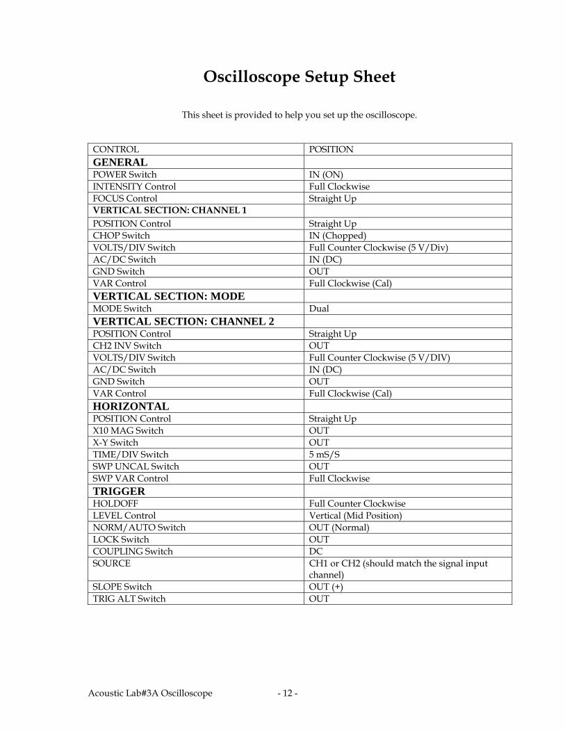
Oscilloscope Setup Sheet

This sheet is provided to help you set up the oscilloscope.

CONTROL POSITION GENERAL POWER Switch IN (ON) INTENSITY Control Full Clockwise FOCUS Control Straight Up VERTICAL SECTION: CHANNEL 1 POSITION Control Straight Up CHOP Switch IN (Chopped) VOLTS/DIV Switch Full Counter Clockwise (5 V/Div) AC/DC Switch IN (DC) GND Switch OUT VAR Control Full Clockwise (Cal) VERTICAL SECTION: MODE MODE Switch Dual VERTICAL SECTION: CHANNEL 2 POSITION Control Straight Up CH2 INV Switch OUT VOLTS/DIV Switch Full Counter Clockwise (5 V/DIV) AC/DC Switch IN (DC) GND Switch OUT VAR Control Full Clockwise (Cal) HORIZONTAL POSITION Control Straight Up X10 MAG Switch OUT X-Y Switch OUT TIME/DIV Switch 5 mS/S SWP UNCAL Switch OUT SWP VAR Control Full Clockwise TRIGGER HOLDOFF Full Counter Clockwise LEVEL Control Vertical (Mid Position) NORM/AUTO Switch OUT (Normal) LOCK Switch OUT COUPLING Switch DC SOURCE CH1 or CH2 (should match the signal input

channel) SLOPE Switch OUT (+) TRIG ALT Switch OUT


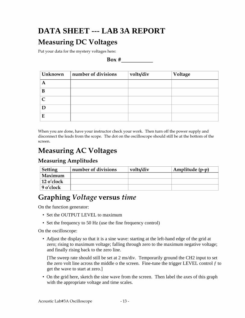
DATA SHEET --- LAB 3A REPORT Measuring DC Voltages

Put your data for the mystery voltages here:

Box #

Unknown number of divisions volts/div Voltage

A

B

C

D

E

When you are done, have your instructor check your work. Then turn off the power supply and disconnect the leads from the scope. The dot on the oscilloscope should still be at the bottom of the screen.

Measuring AC Voltages Measuring Amplitudes

Setting number of divisions volts/div Amplitude (p-p) Maximum 12 o’clock 9 o’clock

Graphing Voltage versus time On the function generator:

• Set the OUTPUT LEVEL to maximum

• Set the frequency to 50 Hz (use the fine frequency control)

On the oscilloscope:

• Adjust the display so that it is a sine wave: starting at the left-hand edge of the grid at zero; rising to maximum voltage; falling through zero to the maximum negative voltage; and finally rising back to the zero line.

[The sweep rate should still be set at 2 ms/div. Temporarily ground the CH2 input to set the zero volt line across the middle o the screen. Fine-tune the trigger LEVEL control ƒ to get the wave to start at zero.]

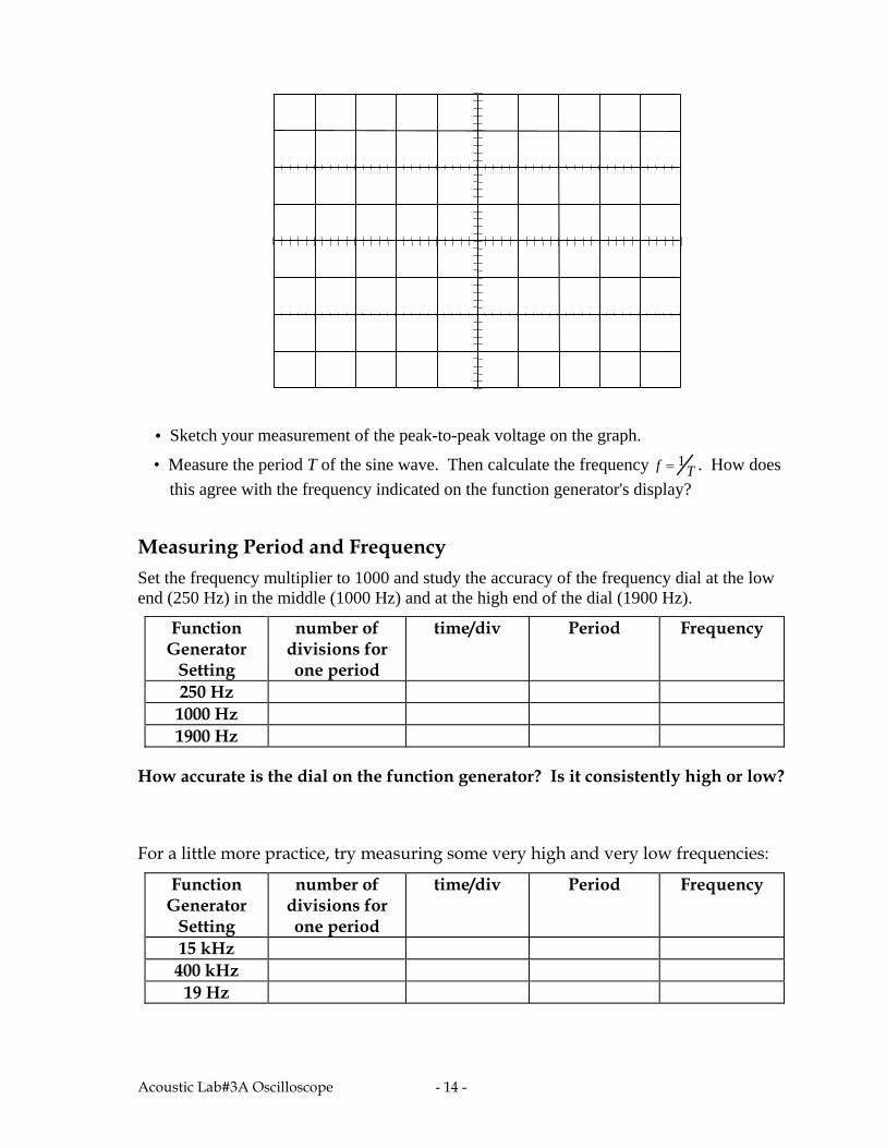
• On the grid here, sketch the sine wave from the screen. Then label the axes of this graph with the appropriate voltage and time scales.


• Sketch your measurement of the peak-to-peak voltage on the graph.

• Measure the period T of the sine wave. Then calculate the frequency f 1

T . How does

this agree with the frequency indicated on the function generator's display?

Measuring Period and Frequency Set the frequency multiplier to 1000 and study the accuracy of the frequency dial at the low end (250 Hz) in the middle (1000 Hz) and at the high end of the dial (1900 Hz).

Function Generator

Setting

number of divisions for one period

time/div Period Frequency

250 Hz 1000 Hz 1900 Hz

How accurate is the dial on the function generator? Is it consistently high or low?

For a little more practice, try measuring some very high and very low frequencies:

Function Generator

Setting

number of divisions for one period

time/div Period Frequency

15 kHz 400 kHz

19 Hz

3B: Resonance in electric LC circuit - 1

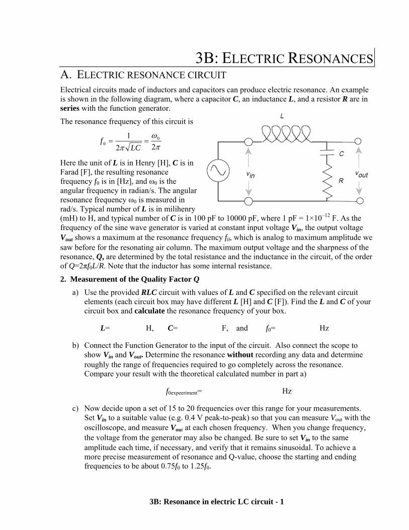
3B: ELECTRIC RESONANCES A. ELECTRIC RESONANCE CIRCUIT Electrical circuits made of inductors and capacitors can produce electric resonance. An example is shown in the following diagram, where a capacitor C, an inductance L, and a resistor R are in series with the function generator.

The resonance frequency of this circuit is

22

1 00

LCf

Here the unit of L is in Henry [H], C is in Farad [F], the resulting resonance frequency f0 is in [Hz], and ω0 is the angular frequency in radian/s. The angular resonance frequency ω0 is measured in rad/s. Typical number of L is in milihenry (mH) to H, and typical number of C is in 100 pF to 10000 pF, where 1 pF = 1×10–12 F. As the frequency of the sine wave generator is varied at constant input voltage Vin, the output voltage Vout shows a maximum at the resonance frequency f0, which is analog to maximum amplitude we saw before for the resonating air column. The maximum output voltage and the sharpness of the resonance, Q, are determined by the total resistance and the inductance in the circuit, of the order of Q=2πf0L/R. Note that the inductor has some internal resistance.

2. Measurement of the Quality Factor Q

a) Use the provided RLC circuit with values of L and C specified on the relevant circuit elements (each circuit box may have different L [H] and C [F]). Find the L and C of your circuit box and calculate the resonance frequency of your box.

L= H, C= F, and f0= Hz

b) Connect the Function Generator to the input of the circuit. Also connect the scope to show Vin and Vout. Determine the resonance without recording any data and determine roughly the range of frequencies required to go completely across the resonance. Compare your result with the theoretical calculated number in part a)

f0expeeriment= Hz

c) Now decide upon a set of 15 to 20 frequencies over this range for your measurements. Set Vin to a suitable value (e.g. 0.4 V peak-to-peak) so that you can measure Vout with the oscilloscope, and measure Vout at each chosen frequency. When you change frequency, the voltage from the generator may also be changed. Be sure to set Vin to the same amplitude each time, if necessary, and verify that it remains sinusoidal. To achieve a more precise measurement of resonance and Q-value, choose the starting and ending frequencies to be about 0.75f0 to 1.25f0.

3B: Resonance in electric LC circuit - 2

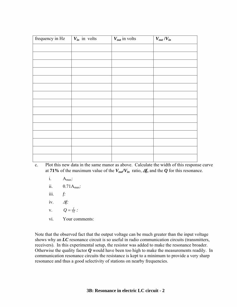
frequency in Hz Vin in volts Vout in volts Vout /Vin

c. Plot this new data in the same manor as above. Calculate the width of this response curve at 71% of the maximum value of the Vout/Vin ratio, f, and the Q for this resonance.

i. Amax:

ii. 0.71Amax:

iii. f:

iv. f:

v. Q f f :

vi. Your comments:

Note that the observed fact that the output voltage can be much greater than the input voltage shows why an LC resonance circuit is so useful in radio communication circuits (transmitters, receivers). In this experimental setup, the resistor was added to make the resonance broader. Otherwise the quality factor Q would have been too high to make the measurements readily. In communication resonance circuits the resistance is kept to a minimum to provide a very sharp resonance and thus a good selectivity of stations on nearby frequencies.

Documents

3A: THE OSCILLOSCOPE Introduction - IU B · PDF file3A: THE OSCILLOSCOPE ... important component of the oscilloscope is the cathode ray tube ... and tell you how to get the oscilloscope