Embed Size (px)
Citation preview

394
Chapter 11
Dimensionality Reduction
There are many sources of data that can be viewed as a large matrix. Wesaw in Chapter 5 how the Web can be represented as a transition matrix. InChapter 9, the utility matrix was a point of focus. And in Chapter 10 weexamined matrices that represent social networks. In many of these matrixapplications, the matrix can be summarized by finding “narrower” matricesthat in some sense are close to the original. These narrow matrices have only asmall number of rows or a small number of columns, and therefore can be usedmuch more efficiently than can the original large matrix. The process of findingthese narrow matrices is called dimensionality reduction.
We saw a preliminary example of dimensionality reduction in Section 9.4.There, we discussed UV-decomposition of a matrix and gave a simple algorithmfor finding this decomposition. Recall that a large matrix M was decomposedinto two matrices U and V whose product UV was approximately M . U had asmall number of columns and V a small number of rows, so each was significantlysmaller than M , and yet together they represented most of the information inM that was useful in predicting ratings of items by individuals.
In this chapter we shall explore the idea of dimensionality reduction inmore detail. We begin with a discussion of eigenvalues and their use in “prin-cipal component analysis” (PCA). We cover singular-value decomposition, amore powerful version of UV-decomposition. Finally, because we are alwaysinterested in the largest data sizes we can handle, we look at another formof decomposition, called CUR-decomposition, which is a variant of singular-value decomposition that keeps the matrices of the decomposition sparse if theoriginal matrix is sparse.
11.1 Eigenvalues and Eigenvectors
We shall assume that you are familiar with the basics of matrix algebra: multi-plication, transpose, determinants, and solving linear equations for example. Inthis section, we shall define eigenvalues and eigenvectors of a symmetric matrix
395
396 CHAPTER 11. DIMENSIONALITY REDUCTION
and show how to find them. Recall a matrix is symmetric if the element in rowi and column j equals the element in row j and column i.
11.1.1 Definitions
Let M be a square matrix. Let λ be a constant and e a nonzero column vectorwith the same number of rows as M . Then λ is an eigenvalue of M and e isthe corresponding eigenvector of M if Me = λe.
If e is an eigenvector of M and c is any constant, then it is also true thatc e is an eigenvector of M with the same eigenvalue. Multiplying a vector by aconstant changes the length of a vector, but not its direction. Thus, to avoidambiguity regarding the length, we shall require that every eigenvector be aunit vector, meaning that the sum of the squares of the components of thevector is 1. Even that is not quite enough to make the eigenvector unique,since we may still multiply by −1 without changing the sum of squares of thecomponents. Thus, we shall normally require that the first nonzero componentof an eigenvector be positive.
Example 11.1 : Let M be the matrix
[
3 22 6
]
One of the eigenvectors of M is
[
1/√
5
2/√
5
]
and its corresponding eigenvalue is 7. The equation
[
3 22 6
] [
1/√
5
2/√
5
]
= 7
[
1/√
5
2/√
5
]
demonstrates the truth of this claim. Note that both sides multiply to
[
7/√
5
14/√
5
]
Also observe that the eigenvector is a unit vector, because (1/√
5)2+(2/√
5)2 =1/5 + 4/5 = 1. 2
11.1.2 Computing Eigenvalues and Eigenvectors
We have already seen one approach to finding an eigenpair (an eigenvalue andits corresponding eigenvector) for a suitable matrix M in Section 5.1: start withany unit vector v of the appropriate length and compute M iv iteratively until it
11.1. EIGENVALUES AND EIGENVECTORS 397
converges.1 When M is a stochastic matrix, the limiting vector is the principal
eigenvector (the eigenvector with the largest eigenvalue), and its correspondingeigenvalue is 1.2 This method for finding the principal eigenvector, called power
iteration, works quite generally, although if the principal eigenvalue (eigenvalueassociated with the principal eigenvector) is not 1, then as i grows, the ratioof M i+1v to M iv approaches the principal eigenvalue while M iv approachesa vector (probably not a unit vector) with the same direction as the principaleigenvector.
We shall take up the generalization of the power-iteration method to find alleigenpairs in Section 11.1.3. However, there is an O(n3)-running-time methodfor computing all the eigenpairs of a symmetric n × n matrix exactly, and thismethod will be presented first. There will always be n eigenpairs, although insome cases, some of the eigenvalues will be identical. The method starts byrestating the equation that defines eigenpairs, Me = λe as (M − λI)e = 0,where
1. I is the n × n identity matrix with 1’s along the main diagonal and 0’selsewhere.
2. 0 is a vector of all 0’s.
A fact of linear algebra is that in order for (M − λI)e = 0 to hold for avector e 6= 0, the determinant of M − λI must be 0. Notice that (M − λI)looks almost like the matrix M , but if M has c in one of its diagonal elements,then (M − λI) has c − λ there. While the determinant of an n × n matrix hasn! terms, it can be computed in various ways in O(n3) time; an example is themethod of “pivotal condensation.”
The determinant of (M − λI) is an nth-degree polynomial in λ, from whichwe can get the n values of λ that are the eigenvalues of M . For each such value,say c, we can then solve the equation Me = c e. There are n equations in nunknowns (the n components of e), but since there is no constant term in anyequation, we can only solve for e to within a constant factor. However, usingany solution, we can normalize it so the sum of the squares of the componentsis 1, thus obtaining the eigenvector that corresponds to eigenvalue c.
Example 11.2 : Let us find the eigenpairs for the 2 × 2 matrix M from Ex-ample 11.1. Recall M =
[
3 22 6
]
Then M − λI is[
3 − λ 22 6 − λ
]
1Recall Mi denotes multiplying by the matrix M i times, as discussed in Section 5.1.2.
2Note that a stochastic matrix is not generally symmetric. Symmetric matrices and
stochastic matrices are two classes of matrices for which eigenpairs exist and can be exploited.
In this chapter, we focus on techniques for symmetric matrices.
398 CHAPTER 11. DIMENSIONALITY REDUCTION
The determinant of this matrix is (3 − λ)(6 − λ) − 4, which we must set to 0.The equation in λ to solve is thus λ2 − 9λ + 14 = 0. The roots of this equationare λ = 7 and λ = 2; the first is the principal eigenvalue, since it is the larger.Let e be the vector of unknowns
[
xy
]
We must solve[
3 22 6
] [
xy
]
= 7
[
xy
]
When we multiply the matrix and vector we get two equations
[
3x + 2y = 7x2x + 6y = 7y
]
Notice that both of these equations really say the same thing: y = 2x. Thus, apossible eigenvector is
[
12
]
But that vector is not a unit vector, since the sum of the squares of its compo-nents is 5, not 1. Thus to get the unit vector in the same direction, we divideeach component by
√5. That is, the principal eigenvector is
[
1/√
5
2/√
5
]
and its eigenvalue is 7. Note that this was the eigenpair we explored in Exam-ple 11.1.
For the second eigenpair, we repeat the above with eigenvalue 2 in place of7. The equation involving the components of e is x = −2y, and the secondeigenvector is
[
2/√
5
−1/√
5
]
Its corresponding eigenvalue is 2, of course. 2
11.1.3 Finding Eigenpairs by Power Iteration
We now examine the generalization of the process we used in Section 5.1 tofind the principal eigenvector, which in that section was the PageRank vector –all we needed from among the various eigenvectors of the stochastic matrix ofthe Web. We start by computing the principal eigenvector by a slight general-ization of the approach used in Section 5.1. We then modify the matrix to, ineffect, remove the principal eigenvector. The result is a new matrix whose prin-cipal eigenvector is the second eigenvector (eigenvector with the second-largest
11.1. EIGENVALUES AND EIGENVECTORS 399
eigenvalue) of the original matrix. The process proceeds in that manner, re-moving each eigenvector as we find it, and then using power iteration to findthe principal eigenvector of the matrix that remains.
Let M be the matrix whose eigenpairs we would like to find. Start with anynonzero vector x0 and then iterate:
xk+1 :=Mxk
‖Mxk‖
Where ‖N‖ for a matrix or vector N denotes the Frobenius norm, that is, thesquare root of the sum of the squares of the elements of N . We multiply currentvector xk by matrix M until convergence (i.e., ‖xk − xk+1‖ is less than somesmall, chosen constant). Let x be xk for that value of k at which convergenceis obtained. Then x is (approximately) the principal eigenvector of M . Toobtain the corresponding eigenvalue we simply compute λ1 = xT Mx, which isthe equation Mx = λx solved for λ, since x is a unit vector.
Example 11.3 : Start with the matrix from Example 11.2:
M =
[
3 22 6
]
and let us start with x0 a vector with 1 for both components. To compute x1,we multiply Mx0 to get
[
3 22 6
] [
11
]
=
[
58
]
The Frobenius norm of the result is√
52 + 82 =√
89 = 9.434. We obtain x1 bydividing 5 and 8 by 9.434; that is:
x1 =
[
0.5300.848
]
For the next iteration, we compute[
3 22 6
] [
0.5300.848
]
=
[
3.2866.148
]
The Frobenius norm of the result is 6.971, so we divide to obtain
x2 =
[
0.4710.882
]
We are converging toward a normal vector whose second component is twice thefirst. That is, the limiting value of the vector that we obtain by power iterationis the principal eigenvector:
x =
[
0.4470.894
]
400 CHAPTER 11. DIMENSIONALITY REDUCTION
Finally, we compute the principal eigenvalue by
λ = xT Mx =[
0.447 0.894]
[
3 22 6
] [
0.4470.894
]
= 6.993
Recall from Example 11.2 that the true principal eigenvector is 7. Power itera-tion will introduce small errors due either to limited precision, as was the casehere, or due to the fact that we stop the iteration before reaching the exactvalue of the eigenvector. When we computed PageRank, the small inaccura-cies did not matter, but when we try to compute all eigenpairs, inaccuraciesaccumulate if we are not careful. 2
To find the second eigenpair we create a new matrix M∗ = M − λ1xxT .Then, use power iteration on M∗ to compute its largest eigenvalue. The ob-tained x∗ and λ∗ correspond to the second largest eigenvalue and the corre-sponding eigenvector of matrix M .
Intuitively, what we have done is eliminate the influence of a given eigen-vector by setting its associated eigenvalue to zero. The formal justification isthe following two observations. If M∗ = M − λxxT , where x and λ are theeigenpair with the largest eigenvalue, then:
1. x is also eigenvector of M∗ where the corresponding eigenvalue of x is 0.In proof, observe that
M∗x = (M − λxxT )x = Mx− λxxTx = Mx − λx = 0
At the next-to-last step we use the fact that xT x = 1 because x is a unitvector.
2. Conversely, if v and λv are an eigenpair of M other than the first eigenpair(x, λ), then they are also an eigenpair of M∗. In proof:
M∗v = (M∗)T v = (M − λxxT )Tv = MTv − λx(xT v) = MTv = λvv
This sequence of equalities needs the following justifications:
(a) M and MT have the same set of eigenvalues and eigenvectors. Notethat if M is symmetric, then M = MT , but even if M is not sym-metric, the statement is true, although we do not prove it here.
(b) The eigenvectors of a matrix are orthogonal. That is, the dot productof any two distinct eigenvectors of a matrix is 0. We do not provethis statement here.
Example 11.4 : Continuing Example 11.3, we compute
M∗ =
[
3 22 6
]
− 6.993[
0.447 0.894]
[
0.4470.894
]
=
[
3 22 6
]
−[
1.399 2.7872.797 5.587
]
=
[
2.601 −0.797−0.797 0.413
]
We may find the second eigenpair by processing the matrix above as we did theoriginal matrix M . 2

11.1. EIGENVALUES AND EIGENVECTORS 401
11.1.4 The Matrix of Eigenvectors
Suppose we have an n × n matrix M whose eigenvectors, viewed as columnvectors, are e1, e2, . . . , en. Let E be the matrix whose ith column is ei. ThenEET = ET E = I. The explanation is that the eigenvectors of a matrix areorthonormal. That is, they are orthogonal unit vectors.
Example 11.5 : For the matrix M of Example 11.2, the matrix E is
[
2/√
5 1/√
5
−1/√
5 2/√
5
]
ET is therefore[
2/√
5 −1/√
5
1/√
5 2/√
5
]
When we compute EET we get
[
4/5 + 1/5 −2/5 + 2/5−2/5 + 2/5 1/5 + 4/5
]
=
[
1 00 1
]
The calculation is similar when we compute ET E. Notice that the 1’s alongthe main diagonal are the sums of the squares of the components of each of theeigenvectors, which makes sense because they are unit vectors. The 0’s off thediagonal reflect the fact that the entry in the ith row and jth column is thedot product of the ith and jth eigenvectors. Since eigenvectors are orthogonal,these dot products are 0. 2
11.1.5 Exercises for Section 11.1
Exercise 11.1.1 : Find the unit vector in the same direction as the vector[1, 2, 3].
Exercise 11.1.2 : Complete Example 11.4 by computing the principal eigen-vector of the matrix that was constructed in this example. How close to thecorrect solution (from Example 11.2) are you?
Exercise 11.1.3 : For any symmetric 3 × 3 matrix
a − λ b cb d − λ ec e f − λ
there is a cubic equation in λ that says the determinant of this matrix is 0. Interms of a through f , find this equation.
402 CHAPTER 11. DIMENSIONALITY REDUCTION
Exercise 11.1.4 : Find the eigenpairs for the following matrix:
1 1 11 2 31 3 5
using the method of Section 11.1.2.
! Exercise 11.1.5 : Find the eigenpairs for the following matrix:
1 1 11 2 31 3 6
using the method of Section 11.1.2.
Exercise 11.1.6 : For the matrix of Exercise 11.1.4:
(a) Starting with a vector of three 1’s, use power iteration to find an approx-imate value of the principal eigenvector.
(b) Compute an estimate the principal eigenvalue for the matrix.
(c) Construct a new matrix by subtracting out the effect of the principaleigenpair, as in Section 11.1.3.
(d) From your matrix of (c), find the second eigenpair for the original matrixof Exercise 11.1.4.
(e) Repeat (c) and (d) to find the third eigenpair for the original matrix.
Exercise 11.1.7 : Repeat Exercise 11.1.6 for the matrix of Exercise 11.1.5.
11.2 Principal-Component Analysis
Principal-component analysis, or PCA, is a technique for taking a dataset con-sisting of a set of tuples representing points in a high-dimensional space andfinding the directions along which the tuples line up best. The idea is to treatthe set of tuples as a matrix M and find the eigenvectors for MMT or MT M .The matrix of these eigenvectors can be thought of as a rigid rotation in a high-dimensional space. When you apply this transformation to the original data,the axis corresponding to the principal eigenvector is the one along which thepoints are most “spread out,” More precisely, this axis is the one along whichthe variance of the data is maximized. Put another way, the points can best beviewed as lying along this axis, with small deviations from this axis. Likewise,the axis corresponding to the second eigenvector (the eigenvector correspond-ing to the second-largest eigenvalue) is the axis along which the variance ofdistances from the first axis is greatest, and so on.
11.2. PRINCIPAL-COMPONENT ANALYSIS 403
We can view PCA as a data-mining technique. The high-dimensional datacan be replaced by its projection onto the most important axes. These axesare the ones corresponding to the largest eigenvalues. Thus, the original datais approximated by data with many fewer dimensions, which summarizes wellthe original data.
11.2.1 An Illustrative Example
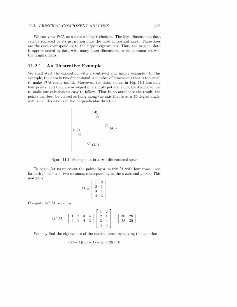
We shall start the exposition with a contrived and simple example. In thisexample, the data is two-dimensional, a number of dimensions that is too smallto make PCA really useful. Moreover, the data, shown in Fig. 11.1 has onlyfour points, and they are arranged in a simple pattern along the 45-degree lineto make our calculations easy to follow. That is, to anticipate the result, thepoints can best be viewed as lying along the axis that is at a 45-degree angle,with small deviations in the perpendicular direction.
(2,1)
(3,4)
(4,3)(1,2)
Figure 11.1: Four points in a two-dimensional space
To begin, let us represent the points by a matrix M with four rows – onefor each point – and two columns, corresponding to the x-axis and y-axis. Thismatrix is
M =
1 22 13 44 3
Compute MT M , which is
MT M =
[
1 2 3 42 1 4 3
]
1 22 13 44 3
=
[
30 2828 30
]
We may find the eigenvalues of the matrix above by solving the equation
(30 − λ)(30 − λ) − 28 × 28 = 0
404 CHAPTER 11. DIMENSIONALITY REDUCTION
as we did in Example 11.2. Here, the solution is λ = 58 and λ = 2.Following the same procedure as in Example 11.2, we must solve
[
30 2828 30
] [
xy
]
= 58
[
xy
]
When we multiply out the matrix and vector we get two equations[
30x + 28y = 58x28x + 30y = 58y
]
Both equations tell us the same thing: x = y. Thus, the unit eigenvectorcorresponding to the principal eigenvalue 58 is
[
1/√
2
1/√
2
]
For the second eigenvalue, 2, we perform the same process. Multiply out[
30 2828 30
] [
xy
]
= 2
[
xy
]
to get the two equations[
30x + 28y = 2x28x + 30y = 2y
]
Both equations tell us the same thing: x = −y. Thus, the unit eigenvectorcorresponding to the principal eigenvalue 2 is
[
−1/√
2
1/√
2
]
While we promised to write eigenvectors with their first component positive,we choose the opposite here because it makes the transformation of coordinateseasier to follow in this case.
Now, let us construct E, the matrix of eigenvectors for the matrix MT M .Placing the principal eigenvector first, the matrix of eigenvectors is
E =
[
1√
2 −1√
2
1√
2 1√
2
]
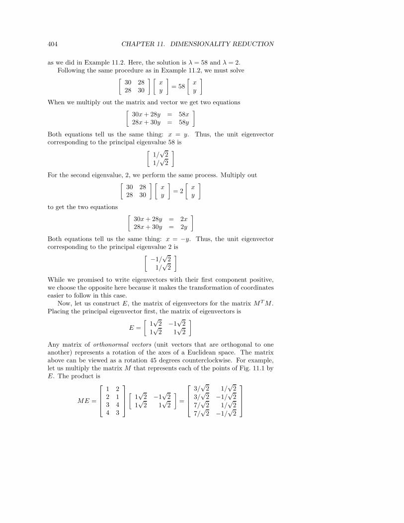
Any matrix of orthonormal vectors (unit vectors that are orthogonal to oneanother) represents a rotation of the axes of a Euclidean space. The matrixabove can be viewed as a rotation 45 degrees counterclockwise. For example,let us multiply the matrix M that represents each of the points of Fig. 11.1 byE. The product is
ME =
1 22 13 44 3
[
1√
2 −1√
2
1√
2 1√
2
]
=
3/√
2 1/√
2
3/√
2 −1/√
2
7/√
2 1/√
2
7/√
2 −1/√
2
11.2. PRINCIPAL-COMPONENT ANALYSIS 405
(2,1)
(3,4)
(4,3)(1,2)
(1.5,1.5)
(3.5,3.5)
Figure 11.2: Figure 11.1 with the axes rotated 45 degrees counterclockwise
For example, the first point, [1, 2], has been transformed into the point
[3√
2, 1/√
2]
If we examine Fig. 11.2, with the dashed line representing the new x-axis, we seethat the projection of the first point onto that axis places it at distance 3/
√2
from the origin. To check that fact, notice that the point of projection for boththe first and second points is [1.5, 1.5] in the original coordinate system, andthe distance from the origin to this point is
√
(1.5)2 + (1.5)2 =√
9/2 = 3/√
2
Moreover, the new y-axis is, of course, perpendicular to the dashed line. Thefirst point is at distance 1/
√2 above the new x-axis in the direction of the
y-axis. That is, the distance between the points [1, 2] and [1.5, 1.5] is
√
(1 − 1.5)2 + (2 − 1.5)2 =√
(−1/2)2 + (1/2)2 =√
1/2 = 1/√
2
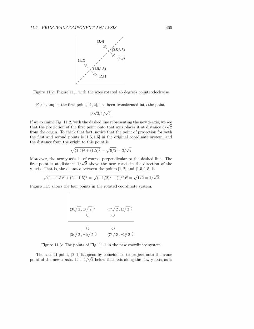
Figure 11.3 shows the four points in the rotated coordinate system.
2 2(3/ , −1/ )
2 2(3/ , 1/ ) 2 2(7/ , 1/ )
2 2(7/ , −1/ )
Figure 11.3: The points of Fig. 11.1 in the new coordinate system
The second point, [2, 1] happens by coincidence to project onto the samepoint of the new x-axis. It is 1/
√2 below that axis along the new y-axis, as is
406 CHAPTER 11. DIMENSIONALITY REDUCTION
confirmed by the fact that the second row in the matrix of transformed pointsis [3/
√2,−1/
√2]. The third point, [3, 4] is transformed into [7/
√2, 1/
√2] and
the fourth point, [4, 3], is transformed to [7/√
2,−1/√
2]. That is, they bothproject onto the same point of the new x-axis, and that point is distance 7/
√2
from the origin, while they are 1/√
2 above and below the new x-axis in thedirection of the new y-axis.
11.2.2 Using Eigenvectors for Dimensionality Reduction
From the example we have just worked, we can see a general principle. If M is amatrix whose rows each represent a point in a Euclidean space with any numberof dimensions, we can compute MT M and compute its eigenpairs. Let E bethe matrix whose columns are the eigenvectors, in the order largest eigenvaluefirst. Define the matrix L to have the eigenvalues of MT M along the diagonal,largest first, and 0’s in all other entries. Then, since MT Me = λe = eλ for eacheigenvector e and its corresponding eigenvalue λ, it follows that MT ME = EL.
We observed that ME is the points of M transformed into a new coordi-nate space. In this space, the first axis (the one corresponding to the largesteigenvalue) is the most significant; formally, the variance of points along thataxis is the greatest. The second axis, corresponding to the second eigenpair,is next most significant in the same sense, and the pattern continues for eachof the eigenpairs. If we want to transform M to a space with fewer dimen-sions, then the choice that preserves the most significance is the one that usesthe eigenvectors associated with the largest eigenvalues and ignores the othereigenvalues.
That is, let Ek be the first k columns of E. Then MEk is a k-dimensionalrepresentation of M .
Example 11.6 : Let M be the matrix from Section 11.2.1. This data has onlytwo dimensions, so the only dimensionality reduction we can do is to use k = 1;i.e., project the data onto a one dimensional space. That is, we compute ME1
by
1 22 13 44 3
[
1/√
2
1/√
2
]
=
3/√
2
3/√
2
7/√
2
7/√
2
The effect of this transformation is to replace the points of M by their pro-jections onto the x-axis of Fig. 11.3. While the first two points project to thesame point, as do the third and fourth points, this representation makes thebest possible one-dimensional distinctions among the points. 2
11.2.3 The Matrix of Distances
Let us return to the example of Section 11.2.1, but instead of starting withMT M , let us examine the eigenvalues of MMT . Since our example M has
11.2. PRINCIPAL-COMPONENT ANALYSIS 407
more rows than columns, the latter is a bigger matrix than the former, but ifM had more columns than rows, we would actually get a smaller matrix. Inthe running example, we have
MMT =
1 22 13 44 3
[
1 2 3 42 1 4 3
]
=
5 4 11 104 5 10 1111 10 25 2410 11 24 25
Like MT M , we see that MMT is symmetric. The entry in the ith row andjth column has a simple interpretation; it is the dot product of the vectorsrepresented by the ith and jth points (rows of M).
There is a strong relationship between the eigenvalues of MT M and MMT .Suppose e is an eigenvector of MT M ; that is,
MT Me = λe
Multiply both sides of this equation by M on the left. Then
MMT (Me) = Mλe = λ(Me)
Thus, as long as Me is not the zero vector 0, it will be an eigenvector of MMT
and λ will be an eigenvalue of MMT as well as of MT M .The converse holds as well. That is, if e is an eigenvector of MMT with
corresponding eigenvalue λ, then start with MMTe = λe and multiply on theleft by MT to conclude that MT M(MTe) = λ(MTe). Thus, if MTe is not 0,then λ is also an eigenvalue of MT M .
We might wonder what happens when MTe = 0. In that case, MMTe
is also 0, but e is not 0 because 0 cannot be an eigenvector. However, since0 = λe, we conclude that λ = 0.
We conclude that the eigenvalues of MMT are the eigenvalues of MT Mplus additional 0’s. If the dimension of MMT were less than the dimensionof MT M , then the opposite would be true; the eigenvalues of MT M would bethose of MMT plus additional 0’s.
3/√
116 1/2 7/√
116 1/2
3/√
116 −1/2 7/√
116 −1/2
7/√
116 1/2 −3/√
116 −1/2
7/√
116 −1/2 −3/√
116 1/2
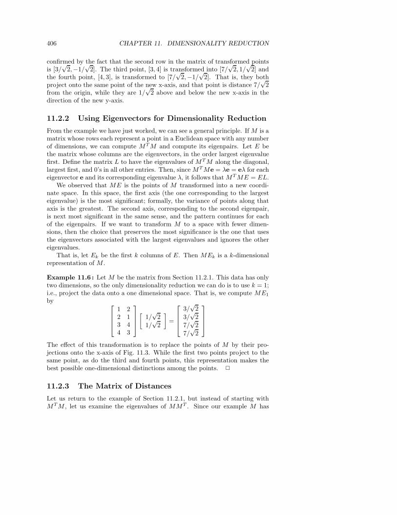
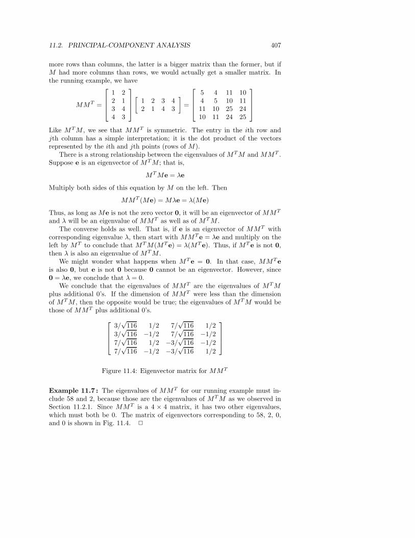
Figure 11.4: Eigenvector matrix for MMT
Example 11.7 : The eigenvalues of MMT for our running example must in-clude 58 and 2, because those are the eigenvalues of MT M as we observed inSection 11.2.1. Since MMT is a 4 × 4 matrix, it has two other eigenvalues,which must both be 0. The matrix of eigenvectors corresponding to 58, 2, 0,and 0 is shown in Fig. 11.4. 2
408 CHAPTER 11. DIMENSIONALITY REDUCTION
11.2.4 Exercises for Section 11.2
Exercise 11.2.1 : Let M be the matrix of data points
1 12 43 94 16
(a) What are MT M and MMT ?
(b) Compute the eigenpairs for MT M .
! (c) What do you expect to be the eigenvalues of MMT ?
! (d) Find the eigenvectors of MMT , using your eigenvalues from part (c).
! Exercise 11.2.2 : Prove that if M is any matrix, then MT M and MMT aresymmetric.
11.3 Singular-Value Decomposition
We now take up a second form of matrix analysis that leads to a low-dimensionalrepresentation of a high-dimensional matrix. This approach, called singular-
value decomposition (SVD), allows an exact representation of any matrix, andalso makes it easy to eliminate the less important parts of that representation toproduce an approximate representation with any desired number of dimensions.Of course the fewer the dimensions we choose, the less accurate will be theapproximation.
We begin with the necessary definitions. Then, we explore the idea that theSVD defines a small number of “concepts” that connect the rows and columnsof the matrix. We show how eliminating the least important concepts gives us asmaller representation that closely approximates the original matrix. Next, wesee how these concepts can be used to query the original matrix more efficiently,and finally we offer an algorithm for performing the SVD itself.
11.3.1 Definition of SVD
Let M be an m×n matrix, and let the rank of M be r. Recall that the rank ofa matrix is the largest number of rows (or equivalently columns) we can choosefor which no nonzero linear combination of the rows is the all-zero vector 0 (wesay a set of such rows or columns is independent). Then we can find matricesU , Σ, and V as shown in Fig. 11.5 with the following properties:
1. U is an m× r column-orthonormal matrix ; that is, each of its columns isa unit vector and the dot product of any two columns is 0.
11.3. SINGULAR-VALUE DECOMPOSITION 409
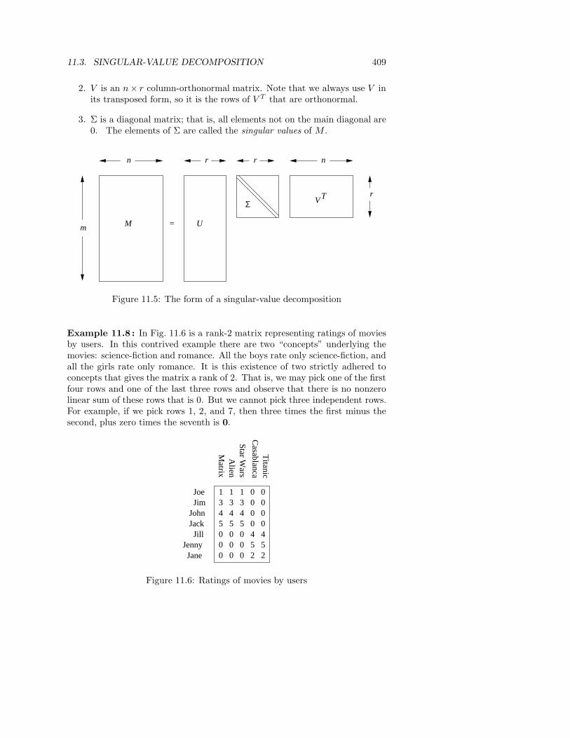
2. V is an n× r column-orthonormal matrix. Note that we always use V inits transposed form, so it is the rows of V T that are orthonormal.
3. Σ is a diagonal matrix; that is, all elements not on the main diagonal are0. The elements of Σ are called the singular values of M .
Mm
n
V T r
U
r
Σ
=
nr
Figure 11.5: The form of a singular-value decomposition
Example 11.8 : In Fig. 11.6 is a rank-2 matrix representing ratings of moviesby users. In this contrived example there are two “concepts” underlying themovies: science-fiction and romance. All the boys rate only science-fiction, andall the girls rate only romance. It is this existence of two strictly adhered toconcepts that gives the matrix a rank of 2. That is, we may pick one of the firstfour rows and one of the last three rows and observe that there is no nonzerolinear sum of these rows that is 0. But we cannot pick three independent rows.For example, if we pick rows 1, 2, and 7, then three times the first minus thesecond, plus zero times the seventh is 0.
1 1 1 0 03 3 3 0 04 4 4 0 05 5 5 0 00 0 0 4 40 0 0 5 50 0 0 2 2
JoeJim
JohnJackJill
JennyJane
Casablanca
Matrix
Titanic
Alien
Star W
ars
Figure 11.6: Ratings of movies by users
410 CHAPTER 11. DIMENSIONALITY REDUCTION
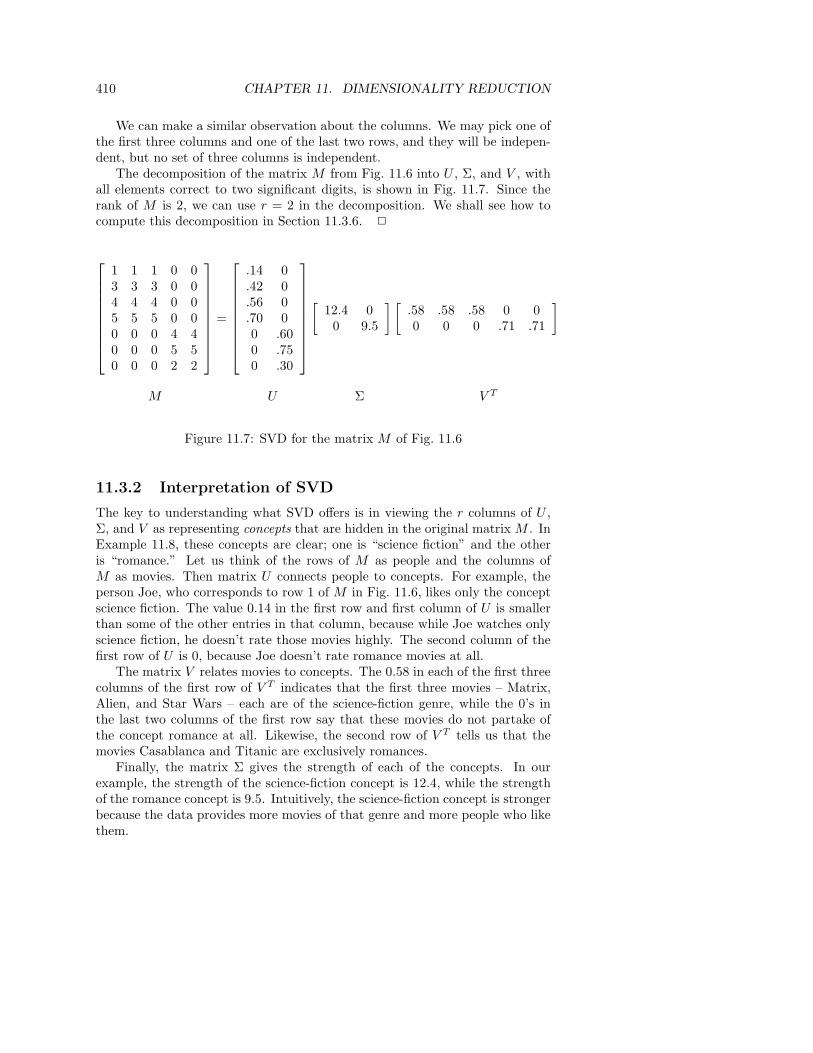
We can make a similar observation about the columns. We may pick one ofthe first three columns and one of the last two rows, and they will be indepen-dent, but no set of three columns is independent.
The decomposition of the matrix M from Fig. 11.6 into U , Σ, and V , withall elements correct to two significant digits, is shown in Fig. 11.7. Since therank of M is 2, we can use r = 2 in the decomposition. We shall see how tocompute this decomposition in Section 11.3.6. 2
1 1 1 0 03 3 3 0 04 4 4 0 05 5 5 0 00 0 0 4 40 0 0 5 50 0 0 2 2
=
.14 0
.42 0
.56 0
.70 00 .600 .750 .30
[
12.4 00 9.5
] [
.58 .58 .58 0 00 0 0 .71 .71
]
M U Σ V T
Figure 11.7: SVD for the matrix M of Fig. 11.6
11.3.2 Interpretation of SVD
The key to understanding what SVD offers is in viewing the r columns of U ,Σ, and V as representing concepts that are hidden in the original matrix M . InExample 11.8, these concepts are clear; one is “science fiction” and the otheris “romance.” Let us think of the rows of M as people and the columns ofM as movies. Then matrix U connects people to concepts. For example, theperson Joe, who corresponds to row 1 of M in Fig. 11.6, likes only the conceptscience fiction. The value 0.14 in the first row and first column of U is smallerthan some of the other entries in that column, because while Joe watches onlyscience fiction, he doesn’t rate those movies highly. The second column of thefirst row of U is 0, because Joe doesn’t rate romance movies at all.
The matrix V relates movies to concepts. The 0.58 in each of the first threecolumns of the first row of V T indicates that the first three movies – Matrix,Alien, and Star Wars – each are of the science-fiction genre, while the 0’s inthe last two columns of the first row say that these movies do not partake ofthe concept romance at all. Likewise, the second row of V T tells us that themovies Casablanca and Titanic are exclusively romances.
Finally, the matrix Σ gives the strength of each of the concepts. In ourexample, the strength of the science-fiction concept is 12.4, while the strengthof the romance concept is 9.5. Intuitively, the science-fiction concept is strongerbecause the data provides more movies of that genre and more people who likethem.

11.3. SINGULAR-VALUE DECOMPOSITION 411
In general, the concepts will not be so clearly delineated. There will be fewer0’s in U and V , although Σ is always a diagonal matrix and will always have0’s off the diagonal. The entities represented by the rows and columns of M(analogous to people and movies in our example) will partake of several differentconcepts to varying degrees. In fact, the decomposition of Example 11.8 wasespecially simple, since the rank of the matrix M was equal to the desirednumber of columns of U , Σ, and V . We were therefore able to get an exactdecomposition of M with only two columns for each of the three matrices U , Σ,and V ; the product UΣV T , if carried out to infinite precision, would be exactlyM . In practice, life is not so simple. When the rank of M is greater than thenumber of columns we want for the matrices U , Σ, and V , the decomposition isnot exact. We need to eliminate from the exact decomposition those columns ofU and V that correspond to the smallest singular values, in order to get the bestapproximation. The following example is a slight modification of Example 11.8that will illustrate the point.
1 1 1 0 03 3 3 0 04 4 4 0 05 5 5 0 00 2 0 4 40 0 0 5 50 1 0 2 2
JoeJim
JohnJackJill
JennyJane
Casablanca
Matrix
Titanic
Alien
Star W
ars
Figure 11.8: The new matrix M ′, with ratings for “Alien” by two additionalraters
Example 11.9 : Figure 11.8 is almost the same as Fig. 11.6, but Jill and Janerated “Alien,” although neither liked it very much. The rank of the matrix inFig. 11.8 is 3; for example the first, sixth, and seventh rows are independent,but you can check that no four rows are independent. Figure 11.9 shows thedecomposition of the matrix from Fig. 11.8.
We have used three columns for U , Σ, and V because they decompose amatrix of rank three. The columns of U and V still correspond to concepts.The first is still “science fiction” and the second is “romance.” It is harder toexplain the third column’s concept, but it doesn’t matter all that much, becauseits weight, as given by the third nonzero entry in Σ, is very low compared withthe weights of the first two concepts. 2
In the next section, we consider eliminating some of the least importantconcepts. For instance, we might want to eliminate the third concept in Ex-
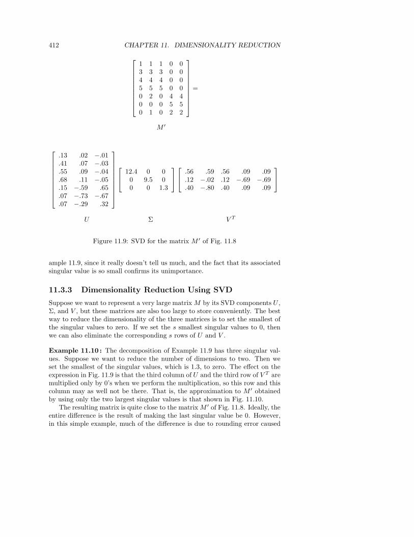
412 CHAPTER 11. DIMENSIONALITY REDUCTION
1 1 1 0 03 3 3 0 04 4 4 0 05 5 5 0 00 2 0 4 40 0 0 5 50 1 0 2 2
=
M ′
.13 .02 −.01
.41 .07 −.03
.55 .09 −.04
.68 .11 −.05
.15 −.59 .65
.07 −.73 −.67
.07 −.29 .32
12.4 0 00 9.5 00 0 1.3
.56 .59 .56 .09 .09
.12 −.02 .12 −.69 −.69
.40 −.80 .40 .09 .09
U Σ V T
Figure 11.9: SVD for the matrix M ′ of Fig. 11.8
ample 11.9, since it really doesn’t tell us much, and the fact that its associatedsingular value is so small confirms its unimportance.
11.3.3 Dimensionality Reduction Using SVD
Suppose we want to represent a very large matrix M by its SVD components U ,Σ, and V , but these matrices are also too large to store conveniently. The bestway to reduce the dimensionality of the three matrices is to set the smallest ofthe singular values to zero. If we set the s smallest singular values to 0, thenwe can also eliminate the corresponding s rows of U and V .
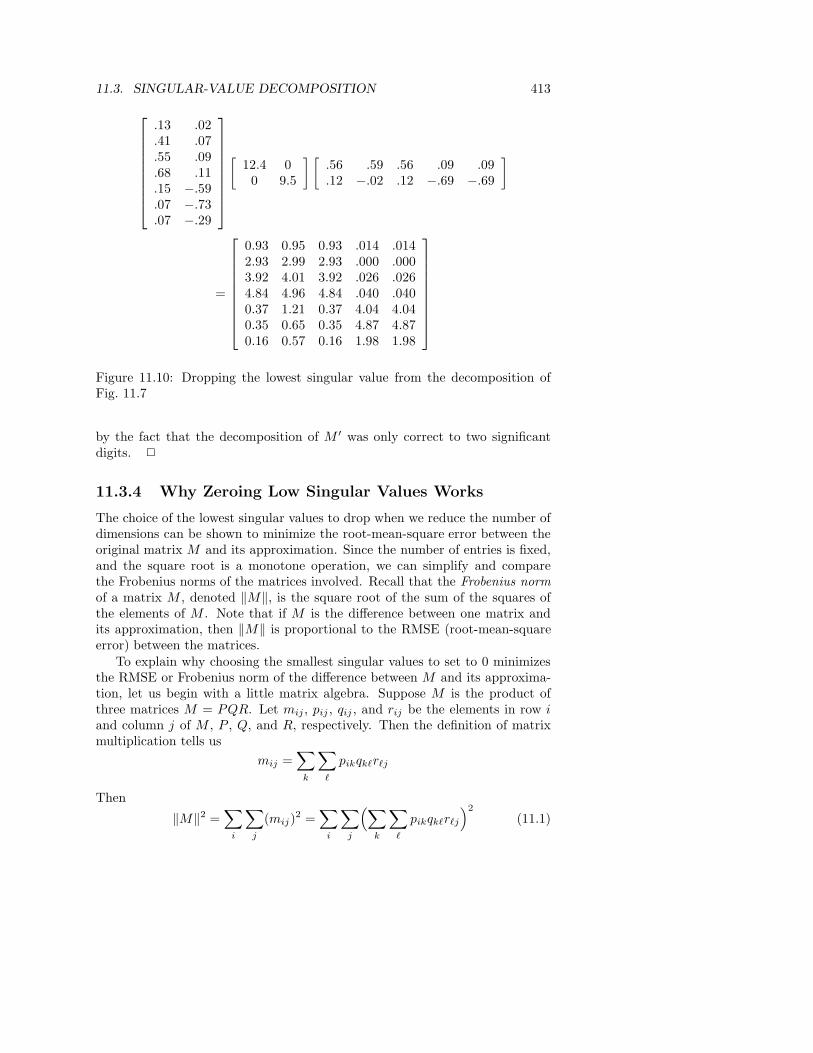
Example 11.10 : The decomposition of Example 11.9 has three singular val-ues. Suppose we want to reduce the number of dimensions to two. Then weset the smallest of the singular values, which is 1.3, to zero. The effect on theexpression in Fig. 11.9 is that the third column of U and the third row of V T aremultiplied only by 0’s when we perform the multiplication, so this row and thiscolumn may as well not be there. That is, the approximation to M ′ obtainedby using only the two largest singular values is that shown in Fig. 11.10.
The resulting matrix is quite close to the matrix M ′ of Fig. 11.8. Ideally, theentire difference is the result of making the last singular value be 0. However,in this simple example, much of the difference is due to rounding error caused
11.3. SINGULAR-VALUE DECOMPOSITION 413
.13 .02
.41 .07
.55 .09
.68 .11
.15 −.59
.07 −.73
.07 −.29
[
12.4 00 9.5
] [
.56 .59 .56 .09 .09
.12 −.02 .12 −.69 −.69
]
=
0.93 0.95 0.93 .014 .0142.93 2.99 2.93 .000 .0003.92 4.01 3.92 .026 .0264.84 4.96 4.84 .040 .0400.37 1.21 0.37 4.04 4.040.35 0.65 0.35 4.87 4.870.16 0.57 0.16 1.98 1.98
Figure 11.10: Dropping the lowest singular value from the decomposition ofFig. 11.7
by the fact that the decomposition of M ′ was only correct to two significantdigits. 2
11.3.4 Why Zeroing Low Singular Values Works
The choice of the lowest singular values to drop when we reduce the number ofdimensions can be shown to minimize the root-mean-square error between theoriginal matrix M and its approximation. Since the number of entries is fixed,and the square root is a monotone operation, we can simplify and comparethe Frobenius norms of the matrices involved. Recall that the Frobenius norm
of a matrix M , denoted ‖M‖, is the square root of the sum of the squares ofthe elements of M . Note that if M is the difference between one matrix andits approximation, then ‖M‖ is proportional to the RMSE (root-mean-squareerror) between the matrices.
To explain why choosing the smallest singular values to set to 0 minimizesthe RMSE or Frobenius norm of the difference between M and its approxima-tion, let us begin with a little matrix algebra. Suppose M is the product ofthree matrices M = PQR. Let mij , pij , qij , and rij be the elements in row iand column j of M , P , Q, and R, respectively. Then the definition of matrixmultiplication tells us
mij =∑
k
∑
ℓ
pikqkℓrℓj
Then
‖M‖2 =∑
i
∑
j
(mij)2 =
∑
i
∑
j
(
∑
k
∑
ℓ
pikqkℓrℓj
)2
(11.1)
414 CHAPTER 11. DIMENSIONALITY REDUCTION
How Many Singular Values Should We Retain?
A useful rule of thumb is to retain enough singular values to make up90% of the energy in Σ. That is, the sum of the squares of the retainedsingular values should be at least 90% of the sum of the squares of all thesingular values. In Example 11.10, the total energy is (12.4)2 + (9.5)2 +(1.3)2 = 245.70, while the retained energy is (12.4)2 + (9.5)2 = 244.01.Thus, we have retained over 99% of the energy. However, were we toeliminate the second singular value, 9.5, the retained energy would beonly (12.4)2/245.70 or about 63%.
When we square a sum of terms, as we do on the right side of Equation 11.1, weeffectively create two copies of the sum (with different indices of summation)and multiply each term of the first sum by each term of the second sum. Thatis,
(
∑
k
∑
ℓ
pikqkℓrℓj
)2
=∑
k
∑
ℓ
∑
m
∑
n
pikqkℓrℓjpinqnmrmj
we can thus rewrite Equation 11.1 as
‖M‖2 =∑
i
∑
j
∑
k
∑
ℓ
∑
n
∑
m
pikqkℓrℓjpinqnmrmj (11.2)
Now, let us examine the case where P , Q, and R are really the SVD of M .That is, P is a column-orthonormal matrix, Q is a diagonal matrix, and R isthe transpose of a column-orthonormal matrix. That is, R is row-orthonormal;its rows are unit vectors and the dot product of any two different rows is 0. Tobegin, since Q is a diagonal matrix, qkℓ and qnm will be zero unless k = ℓ andn = m. We can thus drop the summations for ℓ and m in Equation 11.2 andset k = ℓ and n = m. That is, Equation 11.2 becomes
‖M‖2 =∑
i
∑
j
∑
k
∑
n
pikqkkrkjpinqnnrnj (11.3)
Next, reorder the summation, so i is the innermost sum. Equation 11.3 hasonly two factors pik and pin that involve i; all other factors are constants as faras summation over i is concerned. Since P is column-orthonormal, We knowthat
∑
i pikpin is 1 if k = n and 0 otherwise. That is, in Equation 11.3 we canset k = n, drop the factors pik and pin, and eliminate the sums over i and n,yielding
‖M‖2 =∑
j
∑
k
qkkrkjqkkrkj (11.4)
Since R is row-orthonormal,∑
j rkjrkj is 1. Thus, we can eliminate theterms rkj and the sum over j, leaving a very simple formula for the Frobenius
11.3. SINGULAR-VALUE DECOMPOSITION 415
norm:
‖M‖2 =∑
k
(qkk)2 (11.5)
Next, let us apply this formula to a matrix M whose SVD is M = UΣV T .Let the ith diagonal element of Σ be σi, and suppose we preserve the first nof the r diagonal elements of Σ, setting the rest to 0. Let Σ′ be the resultingdiagonal matrix. Let M ′ = UΣ′V T be the resulting approximation to M . ThenM − M ′ = U(Σ − Σ′)V T is the matrix giving the errors that result from ourapproximation.
If we apply Equation 11.5 to the matrix M − M ′, we see that ‖M − M ′‖2
equals the sum of the squares of the diagonal elements of Σ − Σ′. But Σ − Σ′
has 0 for the first n diagonal elements and σi for the ith diagonal element,where n < i ≤ r. That is, ‖M −M ′‖2 is the sum of the squares of the elementsof Σ that were set to 0. To minimize ‖M − M ′‖2, pick those elements to bethe smallest in Σ. So doing gives the least possible value of ‖M − M ′‖2 underthe constraint that we preserve n of the diagonal elements, and it thereforeminimizes the RMSE under the same constraint.
11.3.5 Querying Using Concepts
In this section we shall look at how SVD can help us answer certain queriesefficiently, with good accuracy. Let us assume for example that we have decom-posed our original movie-rating data (the rank-2 data of Fig. 11.6) into the SVDform of Fig. 11.7. Quincy is not one of the people represented by the originalmatrix, but he wants to use the system to know what movies he would like. Hehas only seen one movie, Matrix, and rated it 4. Thus, we can represent Quincyby the vector q = [4, 0, 0, 0, 0], as if this were one of the rows of the originalmatrix.
If we used a collaborative-filtering approach, we would try to compareQuincy with the other users represented in the original matrix M . Instead,we can map Quincy into “concept space” by multiplying him by the matrix Vof the decomposition. We find qV = [2.32, 0].3 That is to say, Quincy is highin science-fiction interest, and not at all interested in romance.
We now have a representation of Quincy in concept space, derived from, butdifferent from his representation in the original “movie space.” One useful thingwe can do is to map his representation back into movie space by multiplying[2.32, 0] by V T . This product is [1.35, 1.35, 1.35, 0, 0]. It suggests that Quincywould like Alien and Star Wars, but not Casablanca or Titanic.
Another sort of query we can perform in concept space is to find users similarto Quincy. We can use V to map all users into concept space. For example,Joe maps to [1.74, 0], and Jill maps to [0, 5.68]. Notice that in this simpleexample, all users are either 100% science-fiction fans or 100% romance fans, soeach vector has a zero in one component. In reality, people are more complex,
3Note that Fig. 11.7 shows VT , while this multiplication requires V .
416 CHAPTER 11. DIMENSIONALITY REDUCTION
and they will have different, but nonzero, levels of interest in various concepts.In general, we can measure the similarity of users by their cosine distance inconcept space.
Example 11.11 : For the case introduced above, note that the concept vectorsfor Quincy and Joe, which are [2.32, 0] and [1.74, 0], respectively, are not thesame, but they have exactly the same direction. That is, their cosine distanceis 0. On the other hand, the vectors for Quincy and Jill, which are [2.32, 0] and[0, 5.68], respectively, have a dot product of 0, and therefore their angle is 90degrees. That is, their cosine distance is 1, the maximum possible. 2
11.3.6 Computing the SVD of a Matrix
The SVD of a matrix M is strongly connected to the eigenvalues of the symmet-ric matrices MT M and MMT . This relationship allows us to obtain the SVDof M from the eigenpairs of the latter two matrices. To begin the explanation,start with M = UΣV T , the expression for the SVD of M . Then
MT = (UΣV T )T = (V T )T ΣT UT = V ΣT UT
Since Σ is a diagonal matrix, transposing it has no effect. Thus, MT = V ΣUT .
Now, MT M = V ΣUT UΣV T . Remember that U is an orthonormal matrix,so UT U is the identity matrix of the appropriate size. That is,
MT M = V Σ2V T
Multiply both sides of this equation on the left by V to get
MT MV = V Σ2V T V
Since V is also an orthonormal matrix, we know that V T V is the identity. Thus
MT MV = V Σ2 (11.6)
Since Σ is a diagonal matrix, Σ2 is also a diagonal matrix whose entry in theith row and column is the square of the entry in the same position of Σ. Now,Equation (11.6) should be familiar. It says that V is the matrix of eigenvectorsof MT M and Σ2 is the diagonal matrix whose entries are the correspondingeigenvalues.
Thus, the same algorithm that computes the eigenpairs for MT M gives usthe matrix V for the SVD of M itself. It also gives us the singular values forthis SVD; just take the square roots of the eigenvalues for MT M .
Only U remains to be computed, but it can be found in the same way wefound V . Start with
MMT = UΣV T (UΣV T )T = UΣV T V ΣUT = UΣ2UT
11.3. SINGULAR-VALUE DECOMPOSITION 417
Then by a series of manipulations analogous to the above, we learn that
MMT U = UΣ2
That is, U is the matrix of eigenvectors of MMT .A small detail needs to be explained concerning U and V . Each of these
matrices have r columns, while MT M is an n×n matrix and MMT is an m×mmatrix. Both n and m are at least as large as r. Thus, MT M and MMT shouldhave an additional n− r and m− r eigenpairs, respectively, and these pairs donot show up in U , V , and Σ. Since the rank of M is r, all other eigenvalueswill be 0, and these are not useful.
11.3.7 Exercises for Section 11.3
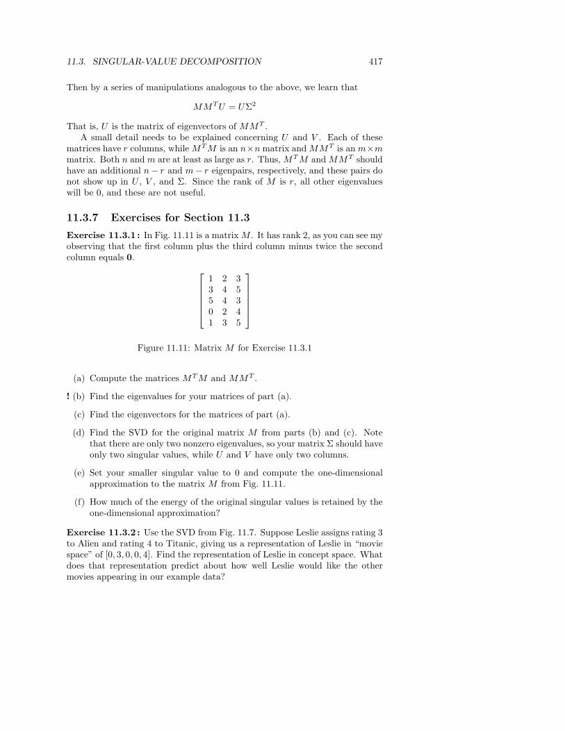
Exercise 11.3.1 : In Fig. 11.11 is a matrix M . It has rank 2, as you can see myobserving that the first column plus the third column minus twice the secondcolumn equals 0.
1 2 33 4 55 4 30 2 41 3 5
Figure 11.11: Matrix M for Exercise 11.3.1
(a) Compute the matrices MT M and MMT .
! (b) Find the eigenvalues for your matrices of part (a).
(c) Find the eigenvectors for the matrices of part (a).
(d) Find the SVD for the original matrix M from parts (b) and (c). Notethat there are only two nonzero eigenvalues, so your matrix Σ should haveonly two singular values, while U and V have only two columns.
(e) Set your smaller singular value to 0 and compute the one-dimensionalapproximation to the matrix M from Fig. 11.11.
(f) How much of the energy of the original singular values is retained by theone-dimensional approximation?
Exercise 11.3.2 : Use the SVD from Fig. 11.7. Suppose Leslie assigns rating 3to Alien and rating 4 to Titanic, giving us a representation of Leslie in “moviespace” of [0, 3, 0, 0, 4]. Find the representation of Leslie in concept space. Whatdoes that representation predict about how well Leslie would like the othermovies appearing in our example data?
418 CHAPTER 11. DIMENSIONALITY REDUCTION
! Exercise 11.3.3 : Demonstrate that the rank of the matrix in Fig. 11.8 is 3.
! Exercise 11.3.4 : Section 11.3.5 showed how to guess the movies a personwould most like. How would you use a similar technique to guess the peoplethat would most like a given movie, if all you had were the ratings of that movieby a few people?
11.4 CUR Decomposition
There is a problem with SVD that does not show up in the running exampleof Section 11.3. In large-data applications, it is normal for the matrix M beingdecomposed to be very sparse; that is, most entries are 0. For example, amatrix representing many documents (as rows) and the words they contain (ascolumns) will be sparse, because most words are not present in most documents.Similarly, a matrix of customers and products will be sparse because mostpeople do not buy most products.
We cannot deal with dense matrices that have millions or billions of rowsand/or columns. However, with SVD, even if M is sparse, U and V will bedense.4 Σ, being diagonal, will be sparse, but Σ is usually much smaller thanU and V , so its sparseness does not help.
In this section, we shall consider another approach to decomposition, calledCUR-decomposition. The merit of this approach lies in the fact that if M issparse, then the two large matrices (called C and R for “rows” and “columns”)analogous to U and V in SVD are also sparse. Only the matrix in the middle(analogous to Σ in SVD) is dense, but this matrix is small so the density doesnot hurt too much.
Unlike SVD, which gives an exact decomposition as long as the parameter ris taken to be at least as great as the rank of the matrix M , CUR-decompositionis an approximation no matter how large we make r. There is a theory thatguarantees convergence to M as r gets larger, but typically you have to make rso large to get, say within 1% that the method becomes impractical. Neverthe-less, a decomposition with a relatively small value of r has a good probabilityof being a useful and accurate decomposition.
11.4.1 Definition of CUR
Let M be a matrix of m rows and n columns. Pick a target number of “concepts”r to be used in the decomposition. A CUR-decomposition of M is a randomlychosen set of r columns of M , which form the m× r matrix C, and a randomlychosen set of r rows of M , which form the r×n matrix R. There is also an r× rmatrix U that is constructed from C and R as follows:
4In Fig. 11.7, it happens that U and V have a significant number of 0’s. However, that is
an artifact of the very regular nature of our example matrix M and is not the case in general.
11.4. CUR DECOMPOSITION 419
Why the Pseudoinverse Works
In general suppose a matrix M is equal to a product of matrices XZY .If all the inverses exist, then the rule for inverse of a product tell usM−1 = Y −1Z−1X−1. Since in the case we are interested in, XZY isan SVD, we know X is column-orthonormal and Y is row-orthonormal.In either of these cases, the inverse and the transpose are the same. Thatis, XXT is an identity matrix of the appropriate size, and so is Y Y T .Thus, M−1 = Y T Z−1XT .
We also know Z is a diagonal matrix. If there are no 0’s along thediagonal, then Z−1 is formed from Z by taking the numerical inverse ofeach diagonal element. It is only when there are 0’s along the diagonalof Z that we are unable to find an element for the same position in theinverse such that we can get an identity matrix when we multiply Z byits inverse. That is why we resort to a “pseudoinverse,” accepting thefact that the product ZZ+ will not be an identity matrix, but rather adiagonal matrix where the ith diagonal entry is 1 if the ith element of Zis nonzero and 0 if the ith element of Z is 0.
1. Let W be the r × r matrix that is the intersection of the chosen columnsof C and the chosen rows of R. That is, the element in row i and columnj of W is the element of M whose column is the jth column of C andwhose row is the ith row of R.
2. Compute the SVD of W ; say W = XΣY T .
3. Compute Σ+, the Moore-Penrose pseudoinverse of the diagonal matrixΣ. That is, if the ith diagonal element of Σ is σ 6= 0, then replace it by1/σ. But if the ith element is 0, leave it at 0.
4. Let U = Y (Σ+)2XT .
We shall defer an example to Section 11.4.3, where we illustrate the entire CURprocess, including the important matter of how the matrices C and R shouldbe chosen to make the approximation to M have a small expected value.
11.4.2 Choosing Rows and Columns Properly
Recall that the choice of rows and columns is random. However, this choicemust be biased so that more important rows and columns have a better chanceof being picked. The measure of importance we must use is the square of theFrobenius norm, that is, the sum of the squares of the elements of the row orcolumn. Let f =
∑
i,j m2ij , the square of the Frobenius norm of M . Then each
time we select a row, the probability pi with which we select row i is∑
j m2ij/f .
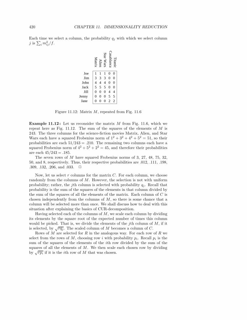
420 CHAPTER 11. DIMENSIONALITY REDUCTION
Each time we select a column, the probability qj with which we select columnj is
∑
i m2ij/f .
1 1 1 0 03 3 3 0 04 4 4 0 05 5 5 0 00 0 0 4 40 0 0 5 50 0 0 2 2
JoeJim
JohnJackJill
JennyJane
Casablanca
Matrix
Titanic
Alien
Star W
ars
Figure 11.12: Matrix M , repeated from Fig. 11.6
Example 11.12 : Let us reconsider the matrix M from Fig. 11.6, which werepeat here as Fig. 11.12. The sum of the squares of the elements of M is243. The three columns for the science-fiction movies Matrix, Alien, and StarWars each have a squared Frobenius norm of 12 + 32 + 42 + 52 = 51, so theirprobabilities are each 51/243 = .210. The remaining two columns each have asquared Frobenius norm of 42 + 52 + 22 = 45, and therefore their probabilitiesare each 45/243 = .185.
The seven rows of M have squared Frobenius norms of 3, 27, 48, 75, 32,50, and 8, respectively. Thus, their respective probabilities are .012, .111, .198,.309, .132, .206, and .033. 2
Now, let us select r columns for the matrix C. For each column, we chooserandomly from the columns of M . However, the selection is not with uniformprobability; rather, the jth column is selected with probability qj . Recall thatprobability is the sum of the squares of the elements in that column divided bythe sum of the squares of all the elements of the matrix. Each column of C ischosen independently from the columns of M , so there is some chance that acolumn will be selected more than once. We shall discuss how to deal with thissituation after explaining the basics of CUR-decomposition.
Having selected each of the columns of M , we scale each column by dividingits elements by the square root of the expected number of times this columnwould be picked. That is, we divide the elements of the jth column of M , if itis selected, by
√rqj . The scaled column of M becomes a column of C.
Rows of M are selected for R in the analogous way. For each row of R weselect from the rows of M , choosing row i with probability pi. Recall pi is thesum of the squares of the elements of the ith row divided by the sum of thesquares of all the elements of M . We then scale each chosen row by dividingby
√rpi if it is the ith row of M that was chosen.
11.4. CUR DECOMPOSITION 421
Example 11.13 : Let r = 2 for our CUR-decomposition. Suppose that ourrandom selection of columns from matrix M of Fig. 11.12 is first Alien (thesecond column) and then Casablanca (the fourth column). The column for Alienis [1, 3, 4, 5, 0, 0, 0]T , and we must scale this column by dividing by
√rq2. Recall
from Example 11.12 that the probability associated with the Alien column is.210, so the division is by
√2 × 0.210 = 0.648. To two decimal places, the
scaled column for Alien is [1.54, 4.63, 6.17, 7.72, 0, 0, 0]T . This column becomesthe first column of C.
The second column of C is constructed by taking the column of M forCasablanca, which is [0, 0, 0, 0, 4, 5, 2]T , and dividing it by
√rp4 =
√2 × 0.185 =
0.430. Thus, the second column of C is [0, 0, 0, 0, 9.30, 11.63, 4.65]T to twodecimal places.
Now, let us choose the rows for R. The most likely rows to be chosen arethose for Jenny and Jack, so let’s suppose these rows are indeed chosen, Jennyfirst. The unscaled rows for R are thus
[
0 0 0 5 55 5 5 0 0
]
To scale the row for Jenny, we note that its associated probability is 0.206, sowe divide by
√2 × 0.206 = 0.454. To scale the row for Jack, whose associated
probability is 0.309, we divide by√
2 × 0.309 = 0.556. Thus, the matrix R is[
0 0 0 11.01 11.018.99 8.99 8.99 0 0
]
2
11.4.3 Constructing the Middle Matrix
Finally, we must construct the matrix U that connects C and R in the decom-position. Recall that U is an r × r matrix. We start the construction of Uwith another matrix of the same size, which we call W . The entry in row i andcolumn j of W is the entry of M whose row is the one from which we selectedthe ith row of R and whose column is the one from which we selected the jthcolumn of C.
Example 11.14 : Let us follow the selections of rows and columns made inExample 11.13. We claim
W =
[
0 55 0
]
The first row of W corresponds to the first row of R, which is the row for Jennyin the matrix M of Fig. 11.12. The 0 in the first column is there because thatis the entry in the row of M for Jenny and the column for Alien; recall that thefirst column of C was constructed from the column of M for Alien. The 5 in thesecond column reflects the 5 in M ’s row for Jenny and column for Casablanca;the latter is the column of M from which the second column of C was derived.
422 CHAPTER 11. DIMENSIONALITY REDUCTION
Similarly, the second row of W is the entries in the row for Jack and columnsfor Alien and Casablanca, respectively. 2
The matrix U is constructed from W by the Moore-Penrose pseudoin-verse described in Section 11.4.1. It consists of taking the SVD of W , sayW = XΣY T , and replacing all nonzero elements in the matrix Σ of singu-lar values by their numerical inverses, to obtain the pseudo-inverse Σ+. ThenU = Y (Σ+)2XT .
Example 11.15 : Let us construct U from the matrix W that we constructedin Example 11.14. First, here is the SVD for W :
W =
[
0 55 0
]
=
[
0 11 0
] [
5 00 5
] [
1 00 1
]
That is, the three matrices on the right are X , Σ, and Y T , respectively. Σ hasno zeros along the diagonal, so each element is replaced by its numerical inverseto get its Moore-Penrose pseudo-inverse:
Σ+ =
[
1/5 00 1/5
]
X and Y are symmetric, so they are their own transposes. Thus,
U = Y (Σ+)2XT =
[
1 00 1
] [
1/5 00 1/5
]2 [
0 11 0
]
=
[
0 1/251/25 0
]
2
11.4.4 The Complete CUR Decomposition
We now have a method to select randomly the three component matrices C,U , and R. Their product will approximate the original matrix M . As wementioned at the beginning of the discussion, the approximation is only for-mally guaranteed to be close when very large numbers of rows and columnsare selected. However, the intuition is that by selecting rows and columns thattend to have high “importance” (i.e., high Frobenius norm), we are extractingthe most significant parts of the original matrix, even with a small number ofrows and columns. As an example, let us see how well we do with the runningexample of this section.
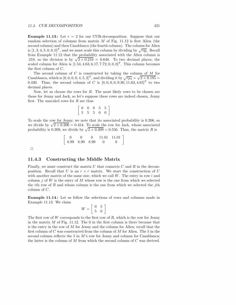
Example 11.16 : For our running example, the decomposition is shown inFig. 11.13. While there is considerable difference between this result and theoriginal matrix M , especially in the science-fiction numbers, the values are inproportion to their originals. This example is much too small, and the selectionof the small numbers of rows and columns was arbitrary rather than random, forus to expect close convergence of the CUR decomposition to the exact values.2
11.4. CUR DECOMPOSITION 423
CUR =
1.54 04.63 06.17 07.72 0
0 9.300 11.630 4.65
[
0 1/251/25 0
] [
0 0 0 11.01 11.018.99 8.99 8.99 0 0
]
=
0.55 0.55 0.55 0 01.67 1.67 1.67 0 02.22 2.22 2.22 0 02.78 2.78 2.78 0 0
0 0 0 4.10 4.100 0 0 5.12 5.120 0 0 2.05 2.05
Figure 11.13: CUR-decomposition of the matrix of Fig. 11.12
11.4.5 Eliminating Duplicate Rows and Columns
It is quite possible that a single row or column is selected more than once.There is no great harm in using the same row twice, although the rank of thematrices of the decomposition will be less than the number of row and columnchoices made. However, it is also possible to combine k rows of R that are eachthe same row of the matrix M into a single row of R, thus leaving R with fewerrows. Likewise, k columns of C that each come from the same column of Mcan be combined into one column of C. However, for either rows or columns,the remaining vector should have each of its elements multiplied by
√k.
When we merge some rows and/or columns, it is possible that R has fewerrows than C has columns, or vice-versa. As a consequence, W will not be asquare matrix. However, we can still take its pseudoinverse by decomposing itinto W = XΣY T , where Σ is now a diagonal matrix with some all-0 rows orcolumns, whichever it has more of. To take the pseudoinverse of such a diagonalmatrix, we treat each element on the diagonal as usual (invert nonzero elementsand leave 0 as it is), but then we must transpose the result.
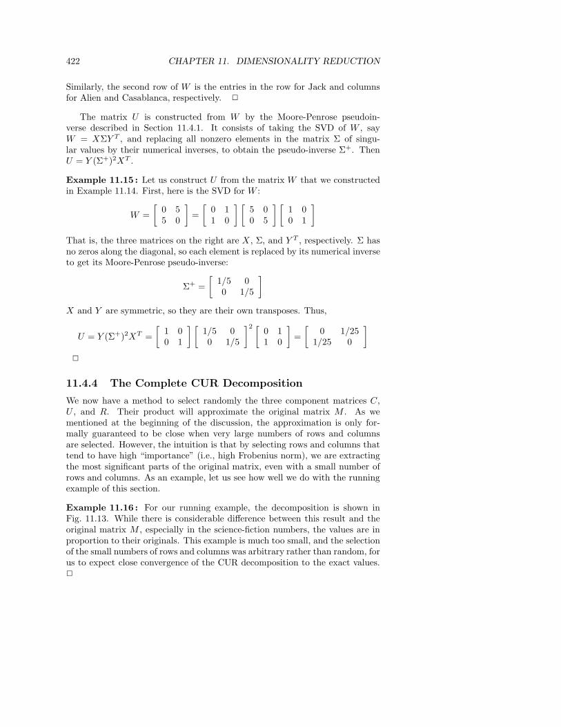
Example 11.17 : Suppose
Σ =
2 0 0 00 0 0 00 0 3 0
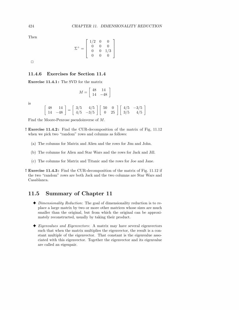
424 CHAPTER 11. DIMENSIONALITY REDUCTION
Then
Σ+ =
1/2 0 00 0 00 0 1/30 0 0
2
11.4.6 Exercises for Section 11.4
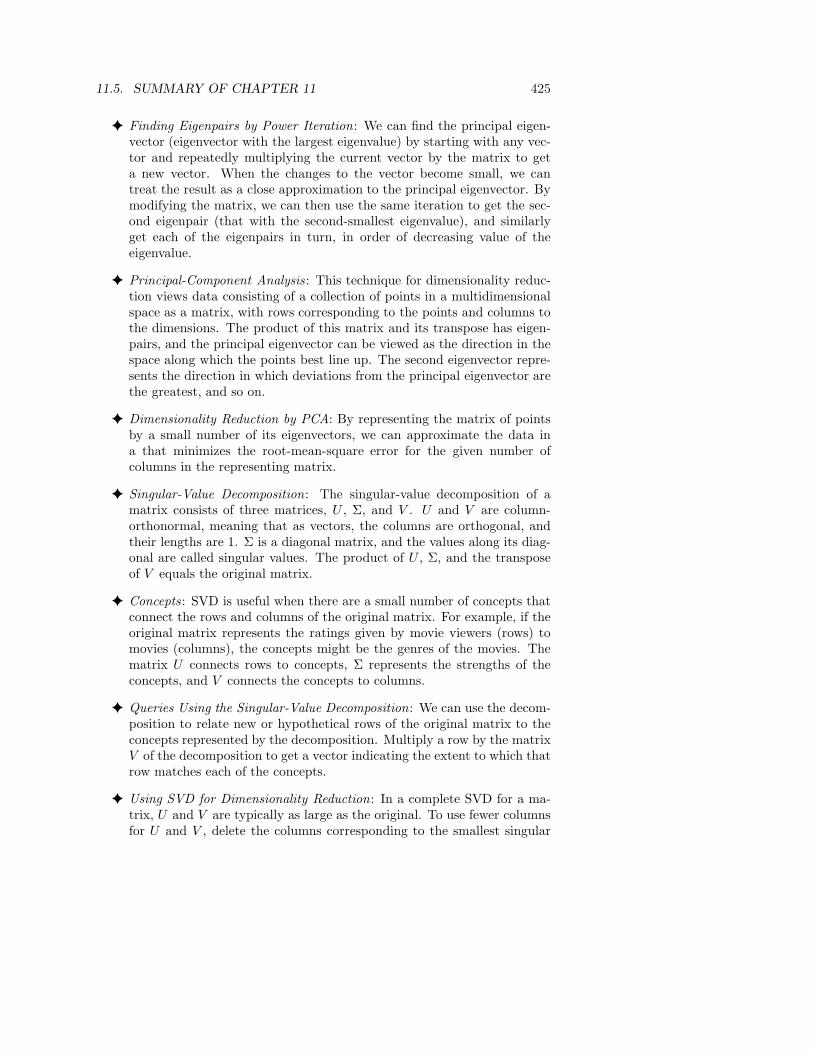
Exercise 11.4.1 : The SVD for the matrix
M =
[
48 1414 −48
]
is[
48 1414 −48
]
=
[
3/5 4/54/5 −3/5
] [
50 00 25
] [
4/5 −3/53/5 4/5
]
Find the Moore-Penrose pseudoinverse of M .
! Exercise 11.4.2 : Find the CUR-decomposition of the matrix of Fig, 11.12when we pick two “random” rows and columns as follows:
(a) The columns for Matrix and Alien and the rows for Jim and John.
(b) The columns for Alien and Star Wars and the rows for Jack and Jill.
(c) The columns for Matrix and Titanic and the rows for Joe and Jane.
! Exercise 11.4.3 : Find the CUR-decomposition of the matrix of Fig. 11.12 ifthe two “random” rows are both Jack and the two columns are Star Wars andCasablanca.
11.5 Summary of Chapter 11
✦ Dimensionality Reduction: The goal of dimensionality reduction is to re-place a large matrix by two or more other matrices whose sizes are muchsmaller than the original, but from which the original can be approxi-mately reconstructed, usually by taking their product.
✦ Eigenvalues and Eigenvectors : A matrix may have several eigenvectorssuch that when the matrix multiplies the eigenvector, the result is a con-stant multiple of the eigenvector. That constant is the eigenvalue asso-ciated with this eigenvector. Together the eigenvector and its eigenvalueare called an eigenpair.
11.5. SUMMARY OF CHAPTER 11 425
✦ Finding Eigenpairs by Power Iteration: We can find the principal eigen-vector (eigenvector with the largest eigenvalue) by starting with any vec-tor and repeatedly multiplying the current vector by the matrix to geta new vector. When the changes to the vector become small, we cantreat the result as a close approximation to the principal eigenvector. Bymodifying the matrix, we can then use the same iteration to get the sec-ond eigenpair (that with the second-smallest eigenvalue), and similarlyget each of the eigenpairs in turn, in order of decreasing value of theeigenvalue.
✦ Principal-Component Analysis : This technique for dimensionality reduc-tion views data consisting of a collection of points in a multidimensionalspace as a matrix, with rows corresponding to the points and columns tothe dimensions. The product of this matrix and its transpose has eigen-pairs, and the principal eigenvector can be viewed as the direction in thespace along which the points best line up. The second eigenvector repre-sents the direction in which deviations from the principal eigenvector arethe greatest, and so on.
✦ Dimensionality Reduction by PCA: By representing the matrix of pointsby a small number of its eigenvectors, we can approximate the data ina that minimizes the root-mean-square error for the given number ofcolumns in the representing matrix.
✦ Singular-Value Decomposition: The singular-value decomposition of amatrix consists of three matrices, U , Σ, and V . U and V are column-orthonormal, meaning that as vectors, the columns are orthogonal, andtheir lengths are 1. Σ is a diagonal matrix, and the values along its diag-onal are called singular values. The product of U , Σ, and the transposeof V equals the original matrix.
✦ Concepts : SVD is useful when there are a small number of concepts thatconnect the rows and columns of the original matrix. For example, if theoriginal matrix represents the ratings given by movie viewers (rows) tomovies (columns), the concepts might be the genres of the movies. Thematrix U connects rows to concepts, Σ represents the strengths of theconcepts, and V connects the concepts to columns.
✦ Queries Using the Singular-Value Decomposition: We can use the decom-position to relate new or hypothetical rows of the original matrix to theconcepts represented by the decomposition. Multiply a row by the matrixV of the decomposition to get a vector indicating the extent to which thatrow matches each of the concepts.
✦ Using SVD for Dimensionality Reduction: In a complete SVD for a ma-trix, U and V are typically as large as the original. To use fewer columnsfor U and V , delete the columns corresponding to the smallest singular
426 CHAPTER 11. DIMENSIONALITY REDUCTION
values from U , V , and Σ. This choice minimizes the error in reconstruct-ing the original matrix from the modified U , Σ, and V .
✦ Decomposing Sparse Matrices : Even in the common case where the givenmatrix is sparse, the matrices constructed by SVD are dense. The CURdecomposition seeks to decompose a sparse matrix into sparse, smallermatrices whose product approximates the original matrix.
✦ CUR Decomposition: This method chooses from a given sparse matrixa set of columns C and a set of rows R, which play the role of U andV T in SVD; the user can pick any number of rows and columns. Thechoice of rows and columns is made randomly with a distribution thatdepends on the Frobenius norm, or the square root of the sum of thesquares of the elements. Between C and R is a square matrix called Uthat is constructed by a pseudo-inverse of the intersection of the chosenrows and columns.
11.6 References for Chapter 11
A well regarded text on matrix algebra is [4].
Principal component analysis was first discussed over a century ago, in [6].
SVD is from [3]. There have been many applications of this idea. Twoworth mentioning are [1] dealing with document analysis and [8] dealing withapplications in Biology.
The CUR decomposition is from [2] and [5]. Our description follows a laterwork [7].
1. S. Deerwester, S.T. Dumais, G.W. Furnas, T.K. Landauer, and R. Harsh-man, “Indexing by latent semantic analysis,” J. American Society for
Information Science 41:6 (1990).
2. P. Drineas, R. Kannan, and M.W. Mahoney, “Fast Monte Carlo algo-rithms for matrices III: Computing a compressed approximate matrixdecomposition,” SIAM J. Computing 36:1 (2006), pp. 184–206.
3. G.H. Golub and W. Kahan, “Calculating the singular values and pseudo-inverse of a matrix,” J. SIAM Series B 2:2 (1965), pp. 205–224.
4. G.H.Golub and C.F. Van Loan, Matrix Computations, JHU Press, 1996.
5. M.W. Mahoney, M. Maggioni, and P. Drineas, Tensor-CUR decomposi-tions For tensor-based data, SIGKDD pp. 327–336, 2006.
6. K. Pearson, “On lines and planes of closest fit to systems of points inspace,” Philosophical Magazine 2:11 (1901), pp. 559–572.

11.6. REFERENCES FOR CHAPTER 11 427
7. J. Sun, Y. Xie, H. Zhang, and C. Faloutsos, “Less is more: compactmatrix decomposition for large sparse graphs,” Proc. SIAM Intl. Conf.
on Data Mining, 2007.
8. M.E. Wall, A. Reichtsteiner and L.M. Rocha, “Singular value decom-position and principal component analysis,” in A Practical Approach to
Microarray Data Analysis (D.P. Berrar, W. Dubitzky, and M. Granzoweds.), pp. 91–109, Kluwer, Norwell, MA, 2003.