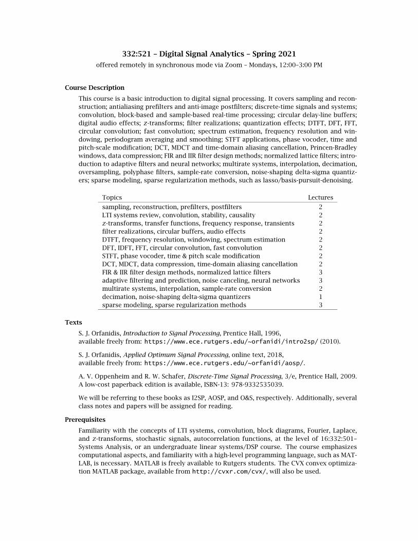
332:521 – Digital Signal Analytics – Spring 2021

offered remotely in synchronous mode via Zoom – Mondays, 12:00–3:00 PM

Course Description

This course is a basic introduction to digital signal processing. It covers sampling and recon-struction; antialiasing prefilters and anti-image postfilters; discrete-time signals and systems;convolution, block-based and sample-based real-time processing; circular delay-line buffers;digital audio effects; z-transforms; filter realizations; quantization effects; DTFT, DFT, FFT,circular convolution; fast convolution; spectrum estimation, frequency resolution and win-dowing, periodogram averaging and smoothing; STFT applications, phase vocoder, time andpitch-scale modification; DCT, MDCT and time-domain aliasing cancellation, Princen-Bradleywindows, data compression; FIR and IIR filter design methods; normalized lattice filters; intro-duction to adaptive filters and neural networks; multirate systems, interpolation, decimation,oversampling, polyphase filters, sample-rate conversion, noise-shaping delta-sigma quantiz-ers; sparse modeling, sparse regularization methods, such as lasso/basis-pursuit-denoising.

Topics Lectures

sampling, reconstruction, prefilters, postfilters 2LTI systems review, convolution, stability, causality 2z-transforms, transfer functions, frequency response, transients 2filter realizations, circular buffers, audio effects 2DTFT, frequency resolution, windowing, spectrum estimation 2DFT, IDFT, FFT, circular convolution, fast convolution 2STFT, phase vocoder, time & pitch scale modification 2DCT, MDCT, data compression, time-domain aliasing cancellation 2FIR & IIR filter design methods, normalized lattice filters 3adaptive filtering and prediction, noise canceling, neural networks 3multirate systems, interpolation, sample-rate conversion 2decimation, noise-shaping delta-sigma quantizers 1sparse modeling, sparse regularization methods 3

Texts

S. J. Orfanidis, Introduction to Signal Processing, Prentice Hall, 1996,available freely from: https://www.ece.rutgers.edu/~orfanidi/intro2sp/ (2010).

S. J. Orfanidis, Applied Optimum Signal Processing, online text, 2018,available freely from: https://www.ece.rutgers.edu/~orfanidi/aosp/.

A. V. Oppenheim and R. W. Schafer, Discrete-Time Signal Processing, 3/e, Prentice Hall, 2009.A low-cost paperback edition is available, ISBN-13: 978-9332535039.

We will be referring to these books as I2SP, AOSP, and O&S, respectively. Additionally, severalclass notes and papers will be assigned for reading.

Prerequisites

Familiarity with the concepts of LTI systems, convolution, block diagrams, Fourier, Laplace,and z-transforms, stochastic signals, autocorrelation functions, at the level of 16:332:501–Systems Analysis, or an undergraduate linear systems/DSP course. The course emphasizescomputational aspects, and familiarity with a high-level programming language, such as MAT-LAB, is necessary. MATLAB is freely available to Rutgers students. The CVX convex optimiza-tion MATLAB package, available from http://cvxr.com/cvx/, will also be used.

Course Requirements

The final grade is based on:

1. Final exam2. Two midterm exams3. Computer projects

Computer Projects

The computer projects are an essential part of the course and may not be skipped or delayed.Project reports and other related materials, such as audio files, should be uploaded to Sakai As-signments by the due date. Please prepare your reports in PDF format using LaTeX (preferably)or Word, and observe the following guidelines:

a. Include a discussion section on the purposes and results of the project.

b. Any numerical and/or theoretical calculations and graphs must be presented in the dis-cussion section.

c. Source code must be attached as an Appendix at the end of the report. (Please neverattach numerical data listings – unless specifically asked.)

d. Please work alone. Collaboration with other students is not allowed.

Project Assigned Due

1. Sampling, prefilter/postfilter design, quantization & dithering 2/01 2/082. Time-constants, bandwidth, filter-lag, zero-lag filters, noise reduction 2/08 2/153. Dynamic range control, compressors, limiters, expanders, duckers 2/15 2/224. Spectrum estimation, periodogram averaging and smoothing 2/22 3/015. Fast convolution, overlap-add & overlap-save methods 3/01 3/086. STFT, phase vocoder, time-scale and pitch-scale modification 3/08 3/227. Data compression, DCT, MDCT, time-domain aliasing cancellation 3/22 3/298. Filter design methods, normalized lattice, quantization effects 3/29 4/059. Adaptive filtering and prediction, LMS and RLS algorithms 4/05 4/19

10. Interpolation, decimation, oversampling, delta-sigma ADCs 4/19 4/2611. Trend extraction, regularized and sparse methods 4/26 5/1012. Sparse modeling, lasso/basis-pursuit-denoising 4/26 5/10

Academic Integrity

By taking this course you agree to work alone on your exams and projects, and you accept andadhere to the Rutgers academic integrity policy described in:

http://academicintegrity.rutgers.edu/academic-integrity-at-rutgers/

Please read also the IEEE code of ethics that should guide your professional life:

https://www.ieee.org/about/corporate/governance/p7-8.html

Instructor

Sophocles J. OrfanidisRoom ELE-230Tel: 848-445-5017e-mail: orfanidi@rci.rutgers.eduOffice hours by email.

Fig.1 – Conventional DSP system.

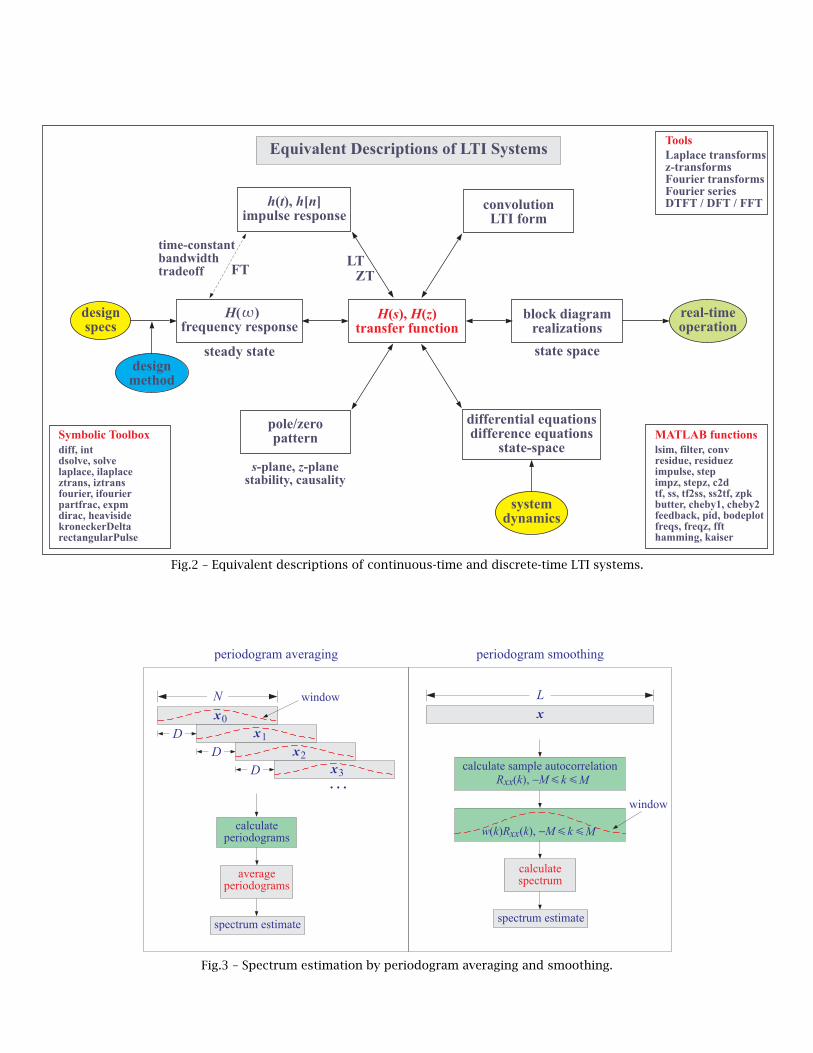
Fig.2 – Equivalent descriptions of continuous-time and discrete-time LTI systems.

Fig.3 – Spectrum estimation by periodogram averaging and smoothing.

Fig.4 – Overlap-add block convolution.

Fig.5 – Overlap-save block convolution.

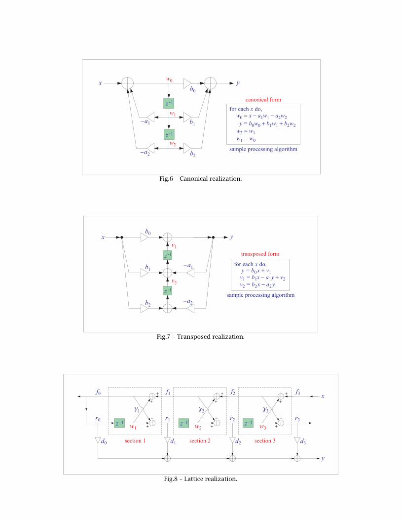
Fig.6 – Canonical realization.

Fig.7 – Transposed realization.

Fig.8 – Lattice realization.

Fig.9 – Optimum Wiener filter and its adaptive implementation.

Fig.10 –Adaptive noise canceling system.

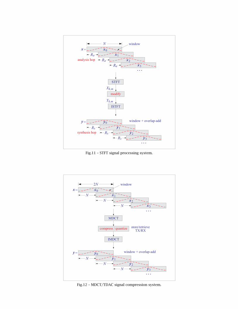
Fig.11 – STFT signal processing system.

Fig.12 – MDCT/TDAC signal compression system.

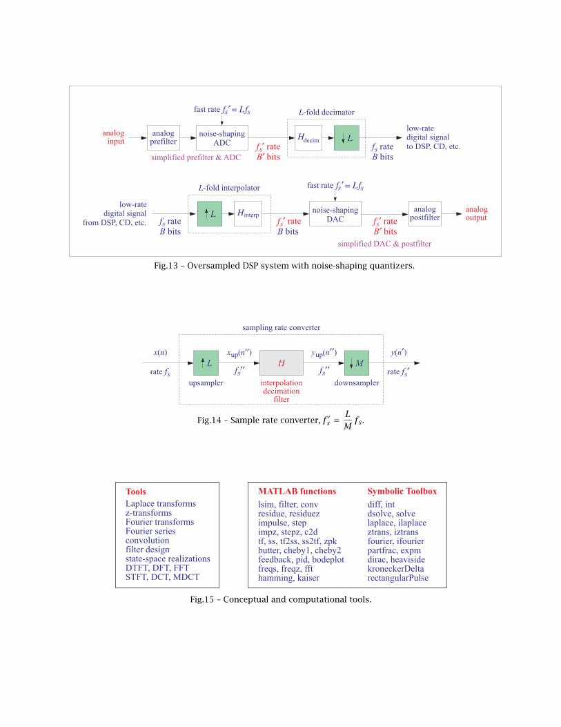
Fig.13 – Oversampled DSP system with noise-shaping quantizers.

Fig.14 – Sample rate converter, f ′s =LMfs.

Fig.15 – Conceptual and computational tools.

0 500 1000 1500 2000

−1

−0.5

0

0.5

1

n

sparse input, s(n)

0 500 1000 1500 2000−20

−10

0

10

20

n

observations, y(n)

0 500 1000 1500 2000

−1

−0.5

0

0.5

1

n

L2, minimum−norm solution, x(n)

error = 71.21 %

0 500 1000 1500 2000

−1

−0.5

0

0.5

1

n

L1, CVX solution, x(n)

error = 2.54 %

0 500 1000 1500 2000

−1

−0.5

0

0.5

1

n

L1, IRLS solution, x(n)

error = 2.54 %

0 500 1000 1500 2000

−1

−0.5

0

0.5

1

n

L0, IRLS solution, x(n)

error = 0.63 %

Fig.16 – Recovered signal based on the L2, L1, and L0 criteria.

(L0): J = ‖b−Ax‖22 + λ‖x‖0 = min

(L1): J = ‖b−Ax‖22 + λ‖x‖1 = min

(L2): J = ‖b−Ax‖22 + λ‖x‖2

2 = min

0 20 40 60 80 100 120 140 160 180 200

−4

−2

0

2

4

6

8

10

exact input, s(n)

n0 20 40 60 80 100 120 140 160 180 200

−4

−2

0

2

4

6

8

10

noisy observations, y(n)

n

SNR = 38 dB

0 20 40 60 80 100 120 140 160 180 200−0.4

−0.2

0

0.2

0.4

0.6

0.8

1

1.2impulse response, h(n)

n0 0.2 0.4 0.6 0.8 1

−40

−30

−20

−10

0

10

20

30

40magnitude response in dB, |H(ω)|

dB

ω / π

0 20 40 60 80 100 120 140 160 180 200

−4

−2

0

2

4

6

8

10

ordinary least−squares solution, x(n), λ = 0

n

percent error = 139.28

0 20 40 60 80 100 120 140 160 180 200

−4

−2

0

2

4

6

8

10

L2 − regularized solution, x(n), λ = 0.01

n

percent error = 77.65

s(n) x(n)

Fig.17a – Sparse deconvolution based on the L2, L1, and L0 criteria.

0 20 40 60 80 100 120 140 160 180 200

−4

−2

0

2

4

6

8

10

L1 − CVX solution, x(n), λ = 0.1

n

percent error = 26.64

0 20 40 60 80 100 120 140 160 180 200

−4

−2

0

2

4

6

8

10

L1 − IRLS solution, x(n), λ = 0.1

n

percent error = 25.57

0 20 40 60 80 100 120 140 160 180 200

−4

−2

0

2

4

6

8

10

L0 − IRLS solution, x(n), λ = 0.1

n

percent error = 0.52

0 4 8 12 16 20

0

10

20

30

40

50

60

iterations, k

perc

ent

L0 − IRLS iteration error, P(k)

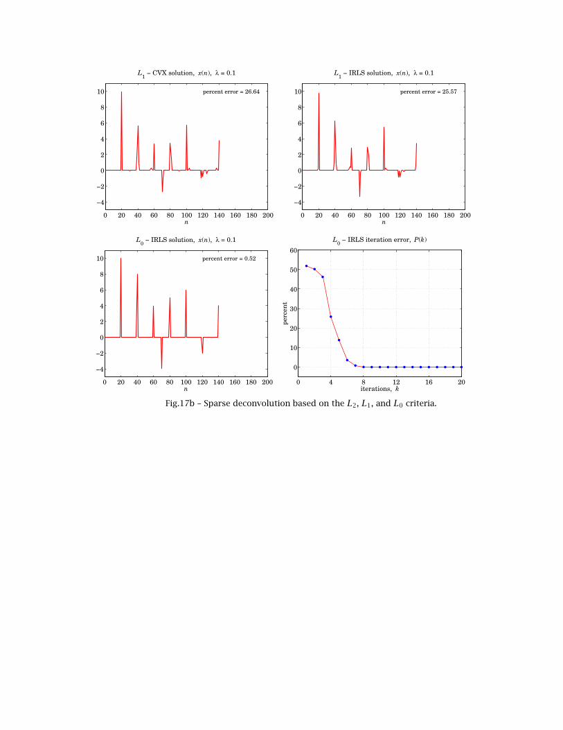
Fig.17b – Sparse deconvolution based on the L2, L1, and L0 criteria.

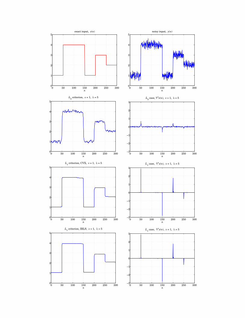
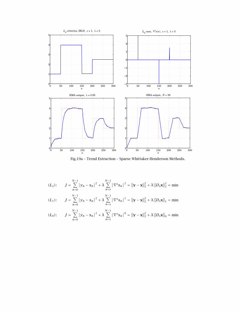
0 50 100 150 200 250 3000

1

2

3

4

5

n

exact input, x(n)

0 50 100 150 200 250 3000

1

2

3

4

5

n

noisy input, y(n)

0 50 100 150 200 250 3000

1

2

3

4

5

n

L2 criterion, s = 1, λ = 5

0 50 100 150 200 250 300−3

−2

−1

0

1

2

3

n

L2 case, ∇sx(n), s = 1, λ = 5

0 50 100 150 200 250 3000

1

2

3

4

5

n

L1 criterion, CVX, s = 1, λ = 5

0 50 100 150 200 250 300−3

−2

−1

0

1

2

3

n

L1 case, ∇sx(n), s = 1, λ = 5

0 50 100 150 200 250 3000

1

2

3

4

5

n

L1 criterion, IRLS, s = 1, λ = 5

0 50 100 150 200 250 300−3

−2

−1

0

1

2

3

n

L1 case, ∇sx(n), s = 1, λ = 5

0 50 100 150 200 250 3000

1

2

3

4

5

n

L0 criterion, IRLS, s = 1, λ = 5

0 50 100 150 200 250 300−3

−2

−1

0

1

2

3

n

L0 case, ∇sx(n), s = 1, λ = 5

0 50 100 150 200 250 3000

1

2

3

4

5

n

EMA output, λ = 0.95

0 50 100 150 200 250 3000

1

2

3

4

5

n

SMA output, N = 39

Fig.19a – Trend Extraction – Sparse Whittaker-Henderson Methods.

(L2): J =N−1∑

n=0

∣∣yn − xn∣∣2 + λ

N−1∑

n=s

∣∣∇sxn∣∣2 = ∥∥y− x

∥∥22 + λ

∥∥Dsx∥∥2

2 = min

(L1): J =N−1∑

n=0

∣∣yn − xn∣∣2 + λ

N−1∑

n=s

∣∣∇sxn∣∣1 = ∥∥y− x

∥∥22 + λ

∥∥Dsx∥∥

1 = min

(L0): J =N−1∑

n=0

∣∣yn − xn∣∣2 + λ

N−1∑

n=s

∣∣∇sxn∣∣0 = ∥∥y− x

∥∥22 + λ

∥∥Dsx∥∥

0 = min

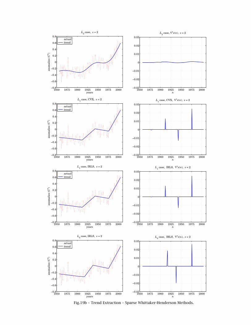
1850 1875 1900 1925 1950 1975 2000−0.8

−0.6

−0.4

−0.2

0

0.2

0.4

0.6

0.8

years

anom

alie

s (C

o )

L2 case, s = 2

actual trend

1850 1875 1900 1925 1950 1975 2000−0.03

−0.02

−0.01

0

0.01

0.02

0.03

n

L2 case, ∇sx(n), s = 2

1850 1875 1900 1925 1950 1975 2000−0.8

−0.6

−0.4

−0.2

0

0.2

0.4

0.6

0.8

years

anom

alie

s (C

o )

L1 case, CVX, s = 2

actual trend

1850 1875 1900 1925 1950 1975 2000−0.03

−0.02

−0.01

0

0.01

0.02

0.03

n

L1 case, CVX, ∇sx(n), s = 2

1850 1875 1900 1925 1950 1975 2000−0.8

−0.6

−0.4

−0.2

0

0.2

0.4

0.6

0.8

years

anom

alie

s (C

o )

L1 case, IRLS, s = 2

actual trend

1850 1875 1900 1925 1950 1975 2000−0.03

−0.02

−0.01

0

0.01

0.02

0.03

n

L1 case, IRLS, ∇sx(n), s = 2

1850 1875 1900 1925 1950 1975 2000−0.8

−0.6

−0.4

−0.2

0

0.2

0.4

0.6

0.8

years

anom

alie

s (C

o )

L0 case, IRLS, s = 2

actual trend

1850 1875 1900 1925 1950 1975 2000−0.03

−0.02

−0.01

0

0.01

0.02

0.03

n

L0 case, IRLS, ∇sx(n), s = 2

Fig.19b – Trend Extraction – Sparse Whittaker-Henderson Methods.