43

3.0 POSITIONING THE NEXRAD STAGEIII CELLS RELATIVE TO THE

DIGITAL ELEVATION MODEL CELLS

In order to define the flow length from each NEXRAD precipitation cell to the

watershed outlets, a mesh of NEXRAD cells must be created in the same coordinate

system as the digital elevation data. This apparently simple task is complicated by the

fact that the original NEXRAD mesh is defined on a spherical earth datum but the

locations of all the radars are recorded in latitudes and longitudes on an ellipsoidal earth

datum. The distinction between these two datums is sufficiently important to require a

careful examination of their definitions and how to make transformations between them.

3.1 GEODETIC (ELLIPSOIDAL) AND GEOCENTRIC (SPHERICAL)

COORDINATES

In a spherical coordinate system, the latitude of a point on the earth's surface is the

angle between the equatorial plane and a line drawn from a point on the earth's surface to

the center of the earth, and the longitude is the angle a plane drawn through a particular

meridian makes with a similar plane drawn through the Greenwich meridian. These are

called geocentric coordinates. But the earth is an oblate spheroid rather than a sphere,

being flattened slightly at the poles compared to the equator such that the polar radius

(6357 km) is about 1/300 shorter than the equatorial radius (6378 km). If the earth is

represented as a sphere of constant radius, such as 6371 km, the "earth surface" or

equivalent of mean sea level is about 7 km below the ocean surface at the equator, and

about 14 km above the ocean surface in the polar regions. To avoid this discrepancy,

geographers represent the earth mathematically by an ellipsoid of rotation with the major

axis of the ellipse in the equatorial plane and the minor axis between the poles. This

change does not alter longitudes but it means that latitudes normally used for mapping

are not defined by a line passing through the center of the earth.

Snyder (1987, p. 13) gives the following definition: "the geographic or geodetic

latitude, which is normally the latitude referred to for a point on the Earth, is the angle

which a line perpendicular to the surface of the ellipsoid at the given point makes with

the plane of the equator. It is slightly greater than the geocentric latitude, except at the

equator and the poles, where it is equal. The geocentric latitude is the angle made by a

line to the center of the ellipsoid with the equatorial plane." For a sphere, the geodetic

44

and geocentric latitudes are identical because a line normal to the surface always passes

through the center but for an ellipsoid they are different.

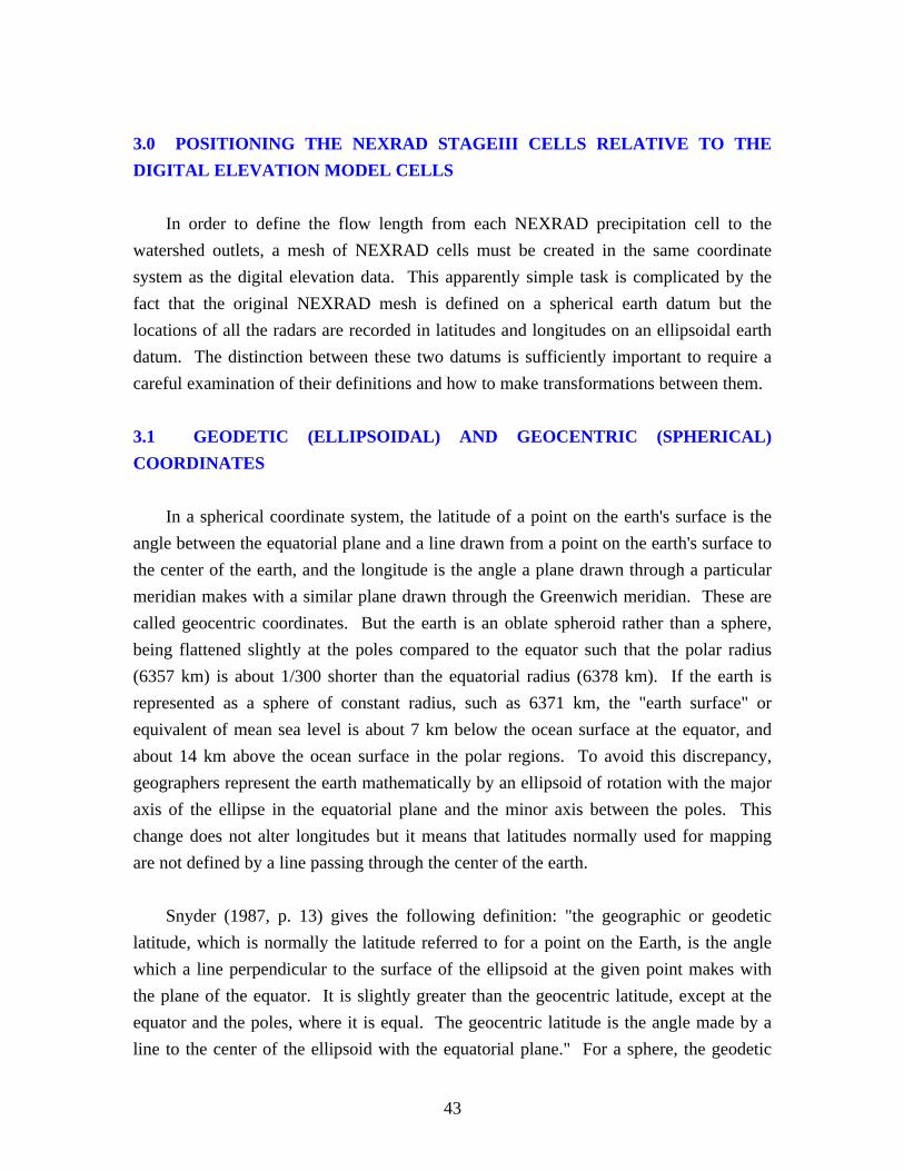
Figure 3.1 is a conceptual diagram illustrating geodetic (φ) and geocentric latitude(φg) of a point B on the earth’s surface where the center of the earth is at point O.

Sphere

Ellipsoid

Rb

a

φφgO

A B (x,y)

C D

Equator

Pole

x

y

Figure 3.1: Geocentric and Geodetic Latitudes

Geometrically, the geocentric latitude of a point B on the earth's surface is given by φg =

angle BOD, and the geodetic latitude by φ = angle BCD, where the line BC is normal to

the surface at the point B and the line BD is tangent to the ellipsoid at point B. Anequivalent point with geocentric latitude φg is located at point A on a sphere of radius R.

It can be seen that the shape of the curve of the ellipse produces a geodetic latitude φgreater than the geocentric latitude φg. The relation between these two latitudes can be

derived in the following manner. The equation for an ellipse is

x2

a 2 + y2

b2 =1 (3.1)

where the coordinates (x,y) of any point B are measured from the center O. By

differentiating Eq. (3.1), the gradient of the surface at B is given by

2x

a2 + 2y

b2

dy

dx= 0

45

ordy

dx= − b2

a2

x

y(3.2)

which is equal to the slope of the tangent line BD. The slope of the line CB which is

normal to the surface and perpendicular to BD is given by the negative inverse of the

slope of BD, or

tan = a2

b2

y

x(3.3)

The line OAB has slope y/x, so the geocentric latitude satisfies the relation

tan g = y

x(3.4)

Thus the geodetic and geocentric latitudes are related by

tan = a2

b2 tan g (3.5)

Snyder (1987, p. 17) presents an equivalent equation to Eq. (3.5) in the form

g = arctan[(1 − e2 )tan ] (3.6)

where the eccentricity e is given by

e2 =1 − b2

a2 (3.7)

It can be verified that Eqs (3.5) and (3.6) are equivalent.

3.1.1 Conversions Between Geodetic and Geocentric Latitudes

As discussed in Section 1.5, three ellipsoids used for mapping in the United States

are GRS 80, Clarke 1866, and WGS 72. The values of the major and minor axis lengths

46

and the corresponding eccentricities of these three ellipsoids are as follows (Snyder,

1987, p.12-13)

GRS 80: a = 6378.137 km, b = 6356.7523 km, e2 = 0.00669438

Clarke 1866: a = 6378.2064 km, b = 6356.5838 km, e2 = 0.006768658

WGS 72: a = 6378.135 km, b = 6356.7505 km, e2 = 0.00669432

By substituting values for a and b for GRS 80 into Eq. (3.5), the following relations arefound between GRS 80 geodetic latitude, φ , and geocentric latitude, φg:

= tan −1(1.00673950tan g) (3.8)

g = tan −1(0.99330562tan ) (3.9)

The simplest connection between the sphere and an ellipsoid is to use either the GRS 80

ellipsoid or the WGS 72 ellipsoid because the NAD 83, WGS 84, and WGS 72 datums

use their respective ellipsoids in a geocentered position. In NAD 27, the Clarke ellipsoid

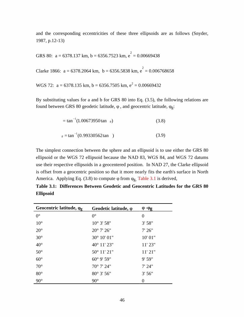
is offset from a geocentric position so that it more nearly fits the earth's surface in NorthAmerica. Applying Eq. (3.8) to compute φ from φg, Table 3.1 is derived,

Table 3.1: Differences Between Geodetic and Geocentric Latitudes for the GRS 80

Ellipsoid

Geocentric latitude, φφg Geodetic latitude, φφ φφ -φφg

0° 0° 0

10° 10° 3' 58'' 3' 58"

20° 20° 7' 26" 7' 26"

30° 30° 10' 01" 10' 01"

40° 40° 11' 23" 11' 23"

50° 50° 11' 21" 11' 21"

60° 60° 9' 59" 9' 59"

70° 70° 7' 24" 7' 24"

80° 80° 3' 56" 3' 56"

90° 90° 0

47

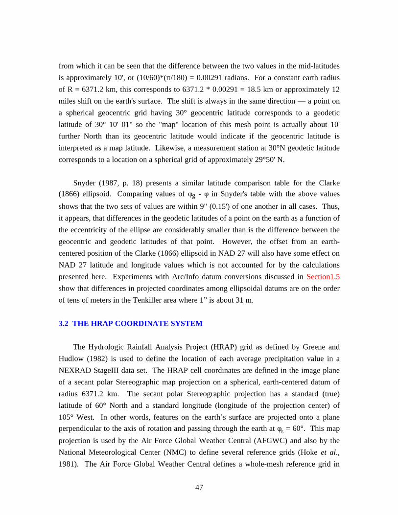
from which it can be seen that the difference between the two values in the mid-latitudes

is approximately 10', or (10/60)*(π/180) = 0.00291 radians. For a constant earth radius

of R = 6371.2 km, this corresponds to 6371.2 * 0.00291 = 18.5 km or approximately 12

miles shift on the earth's surface. The shift is always in the same direction — a point on

a spherical geocentric grid having 30° geocentric latitude corresponds to a geodetic

latitude of 30° 10' 01" so the "map" location of this mesh point is actually about 10'

further North than its geocentric latitude would indicate if the geocentric latitude is

interpreted as a map latitude. Likewise, a measurement station at 30°N geodetic latitude

corresponds to a location on a spherical grid of approximately 29°50' N.

Snyder (1987, p. 18) presents a similar latitude comparison table for the Clarke(1866) ellipsoid. Comparing values of φg - φ in Snyder's table with the above values

shows that the two sets of values are within 9" (0.15') of one another in all cases. Thus,

it appears, that differences in the geodetic latitudes of a point on the earth as a function of

the eccentricity of the ellipse are considerably smaller than is the difference between the

geocentric and geodetic latitudes of that point. However, the offset from an earth-

centered position of the Clarke (1866) ellipsoid in NAD 27 will also have some effect on

NAD 27 latitude and longitude values which is not accounted for by the calculations

presented here. Experiments with Arc/Info datum conversions discussed in Section1.5

show that differences in projected coordinates among ellipsoidal datums are on the order

of tens of meters in the Tenkiller area where 1” is about 31 m.

3.2 THE HRAP COORDINATE SYSTEM

The Hydrologic Rainfall Analysis Project (HRAP) grid as defined by Greene and

Hudlow (1982) is used to define the location of each average precipitation value in a

NEXRAD StageIII data set. The HRAP cell coordinates are defined in the image plane

of a secant polar Stereographic map projection on a spherical, earth-centered datum of

radius 6371.2 km. The secant polar Stereographic projection has a standard (true)

latitude of 60° North and a standard longitude (longitude of the projection center) of

105° West. In other words, features on the earth’s surface are projected onto a plane

perpendicular to the axis of rotation and passing through the earth at φg = 60°. This map

projection is used by the Air Force Global Weather Central (AFGWC) and also by the

National Meteorological Center (NMC) to define several reference grids (Hoke et al.,

1981). The Air Force Global Weather Central defines a whole-mesh reference grid in

48

this map projection and several finer-resolution grids relative to the whole mesh grid. By

definition, the whole-mesh grid length is 381 km. Finer resolution grids are defined as

one-half, one-quarter, one-eighth, and one sixty-fourth of the whole-mesh grid. The

half-mesh grid length is 190.5 km (Hoke et al., 1981). The HRAP grid size is equivalent

to one-eightieth of the whole-mesh grid, resulting in a grid length of 381/80 = 4.7625

km. However, the standard longitude of the Air Force Global Weather Central reference

grids (10° E) is different than the standard longitude for HRAP (105° W) which means

that the orientation of HRAP cells relative to map features is different than that of whole-

mesh grid cells. In other words, HRAP cells do not fall in alignment with the whole-

mesh grid cells. The grid cell lengths cited above are in the projected plane. Lengths in

the projected plane are only equivalent to lengths on the surface of the spherical earth

datum at 60° N.

3.2.1 Forward Transformation from Geocentric to HRAP Coordinates

The procedure for projecting spherical coordinates in degrees on the earth’s surface

to Cartesian coordinates in meters on a flat surface can be thought of in two parts. First,

convert the geographic coordinates in latitude and longitude (φg,λ) into equivalent polar

coordinates (R,λ) on a flat plane. Second, convert the polar coordinates (R,λ) to

Cartesian coordinates (x,y) in the same plane. Finally, a grid mesh is defined in the

projected plane by specifying a point of origin (xo,yo) and then a mesh size and

orientation about that point. The steps are the same when an ellipsoidal datum is used

but the conversion from ellipsoidal coordinates to polar coordinates in a plane is more

complex because the radius of curvature on an ellipsoidal earth varies continuously with

latitude and also varies continuously with direction at any point.

3.2.1.1 From Geographic to Polar Coordinates

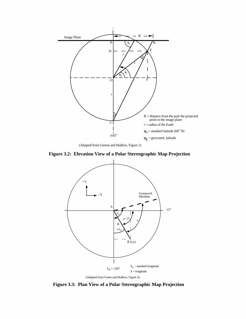
The polar Stereographic projection is an azimuthal projection (projection onto a plane).

Figure3.2 illustrates the geometry of the polar Stereographic map transformation with a

standard latitude of 60° N. A light shining from point C will project point E on the

Earth's surface onto the image plane at point B. In the polar Stereographic projection,

the point B on the image plane can be defined by two parameters, the distance from the

pole R and the longitude (λ) measured from the Greenwich Meridian. An expression for

R as a function of latitude (φg) can be derived from Figure 3.2 .

.

B

C

D E

O

R

r

φg

φο

β

r

r

β

φο

-105°

Image Plane

F

(Adapted from Greene and Hudlow, Figure 1)

φo = standard latitude (60° N)

φg = geocentric latitude

r = radius of the Earth

R = distance from the pole the projected point in the image plane

A

+ X

+ Y

R

B (x,y)

λo = -105°

GreenwichMeridian

λ+ 15°λ

λ-λo

λo

A

λo = standard longitude

λ = longitude

(Adapted from Green and Hudlow, Figure 2)

-15°

Figure 3.2: Elevation View of a Polar Stereographic Map Projection

Figure 3.3: Plan View of a Polar Stereographic Map Projection

50

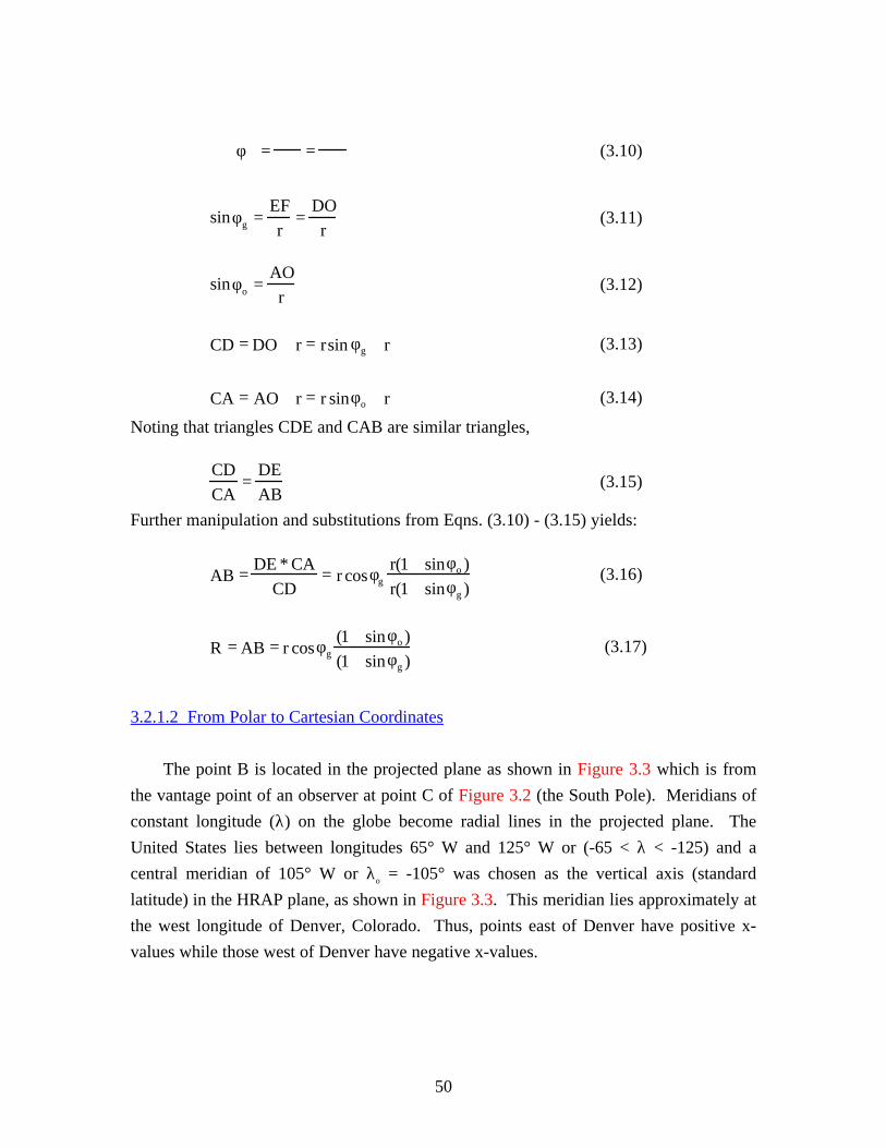
φ = = (3.10)

sinφg =EF

r=

DO

r(3.11)

sinφo =AO

r(3.12)

CD = DO + r = rsin φg + r (3.13)

CA = AO + r = r sinφo + r (3.14)

Noting that triangles CDE and CAB are similar triangles,

CD

CA=

DE

AB(3.15)

Further manipulation and substitutions from Eqns. (3.10) - (3.15) yields:

AB = DE * CA

CD= r cosφg

r(1 + sinφo )

r(1 + sinφg )(3.16)

R = AB = r cosφg

(1 + sinφo )

(1 + sinφg ) (3.17)

3.2.1.2 From Polar to Cartesian Coordinates

The point B is located in the projected plane as shown in Figure 3.3 which is from

the vantage point of an observer at point C of Figure 3.2 (the South Pole). Meridians of

constant longitude (λ) on the globe become radial lines in the projected plane. The

United States lies between longitudes 65° W and 125° W or (-65 < λ < -125) and a

central meridian of 105° W or λo = -105° was chosen as the vertical axis (standard

latitude) in the HRAP plane, as shown in Figure 3.3. This meridian lies approximately at

the west longitude of Denver, Colorado. Thus, points east of Denver have positive x-

values while those west of Denver have negative x-values.

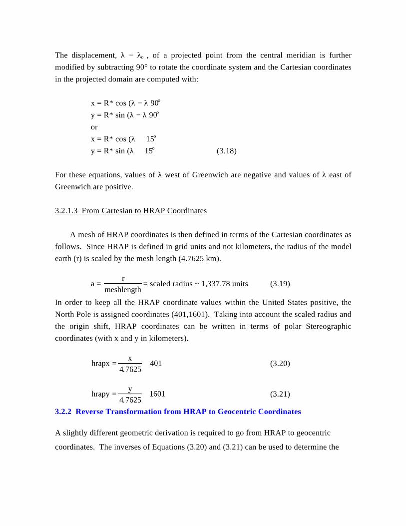
The displacement, λ − λo , of a projected point from the central meridian is furthermodified by subtracting 90° to rotate the coordinate system and the Cartesian coordinatesin the projected domain are computed with:

x = R* cos (λ − λ 90ο )y = R* sin (λ − λ 90ο )orx = R* cos (λ + 15ο )y = R* sin (λ + 15ο ) (3.18)

For these equations, values of λ west of Greenwich are negative and values of λ east ofGreenwich are positive.

3.2.1.3 From Cartesian to HRAP Coordinates

A mesh of HRAP coordinates is then defined in terms of the Cartesian coordinates asfollows. Since HRAP is defined in grid units and not kilometers, the radius of the modelearth (r) is scaled by the mesh length (4.7625 km).

a = r

meshlength= scaled radius ~ 1,337.78 units (3.19)

In order to keep all the HRAP coordinate values within the United States positive, theNorth Pole is assigned coordinates (401,1601). Taking into account the scaled radius andthe origin shift, HRAP coordinates can be written in terms of polar Stereographiccoordinates (with x and y in kilometers).

hrapx =x

4.7625+ 401 (3.20)

hrapy =y

4.7625+1601 (3.21)

3.2.2 Reverse Transformation from HRAP to Geocentric Coordinates

A slightly different geometric derivation is required to go from HRAP to geocentric

coordinates. The inverses of Equations (3.20) and (3.21) can be used to determine the

52

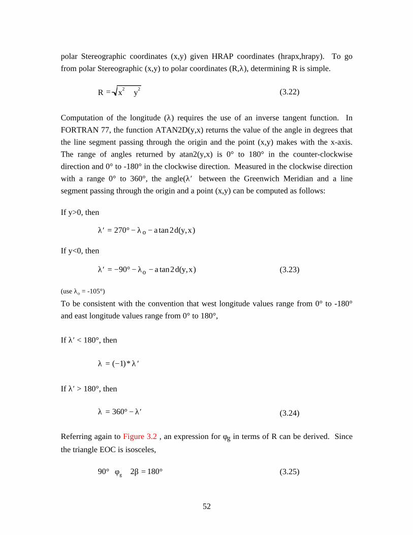
polar Stereographic coordinates (x,y) given HRAP coordinates (hrapx,hrapy). To go

from polar Stereographic (x,y) to polar coordinates (R,λ), determining R is simple.

R = x2 + y

2 (3.22)

Computation of the longitude (λ) requires the use of an inverse tangent function. In

FORTRAN 77, the function ATAN2D(y,x) returns the value of the angle in degrees that

the line segment passing through the origin and the point (x,y) makes with the x-axis.

The range of angles returned by atan2(y,x) is 0° to 180° in the counter-clockwise

direction and 0° to -180° in the clockwise direction. Measured in the clockwise direction

with a range 0° to 360°, the angle(λ′) between the Greenwich Meridian and a line

segment passing through the origin and a point (x,y) can be computed as follows:

If y>0, then

′ λ = 270° − λo − a tan2d(y,x)

If y<0, then

′ λ = −90° − λo − a tan2d(y,x) (3.23)

(use λo = -105°)

To be consistent with the convention that west longitude values range from 0° to -180°

and east longitude values range from 0° to 180°,

If λ′ < 180°, then

λ = (−1)* ′ λ

If λ′ > 180°, then

λ = 360° − ′ λ (3.24)

Referring again to Figure 3.2 , an expression for φg in terms of R can be derived. Since

the triangle EOC is isosceles,

90°+φg + 2β = 180° (3.25)

53

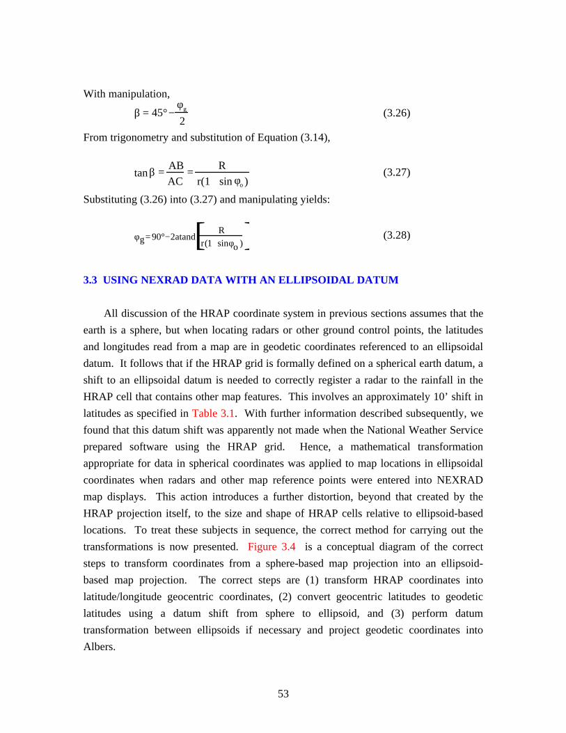
With manipulation,

β = 45°−φg

2(3.26)

From trigonometry and substitution of Equation (3.14),

tanβ = AB

AC= R

r(1+ sin φo )(3.27)

Substituting (3.26) into (3.27) and manipulating yields:

φg=90°−2atandR

r(1+sinφo )[ ] (3.28)

3.3 USING NEXRAD DATA WITH AN ELLIPSOIDAL DATUM

All discussion of the HRAP coordinate system in previous sections assumes that the

earth is a sphere, but when locating radars or other ground control points, the latitudes

and longitudes read from a map are in geodetic coordinates referenced to an ellipsoidal

datum. It follows that if the HRAP grid is formally defined on a spherical earth datum, a

shift to an ellipsoidal datum is needed to correctly register a radar to the rainfall in the

HRAP cell that contains other map features. This involves an approximately 10’ shift in

latitudes as specified in Table 3.1. With further information described subsequently, we

found that this datum shift was apparently not made when the National Weather Service

prepared software using the HRAP grid. Hence, a mathematical transformation

appropriate for data in spherical coordinates was applied to map locations in ellipsoidal

coordinates when radars and other map reference points were entered into NEXRAD

map displays. This action introduces a further distortion, beyond that created by the

HRAP projection itself, to the size and shape of HRAP cells relative to ellipsoid-based

locations. To treat these subjects in sequence, the correct method for carrying out the

transformations is now presented. Figure 3.4 is a conceptual diagram of the correct

steps to transform coordinates from a sphere-based map projection into an ellipsoid-

based map projection. The correct steps are (1) transform HRAP coordinates into

latitude/longitude geocentric coordinates, (2) convert geocentric latitudes to geodetic

latitudes using a datum shift from sphere to ellipsoid, and (3) perform datum

transformation between ellipsoids if necessary and project geodetic coordinates into

Albers.

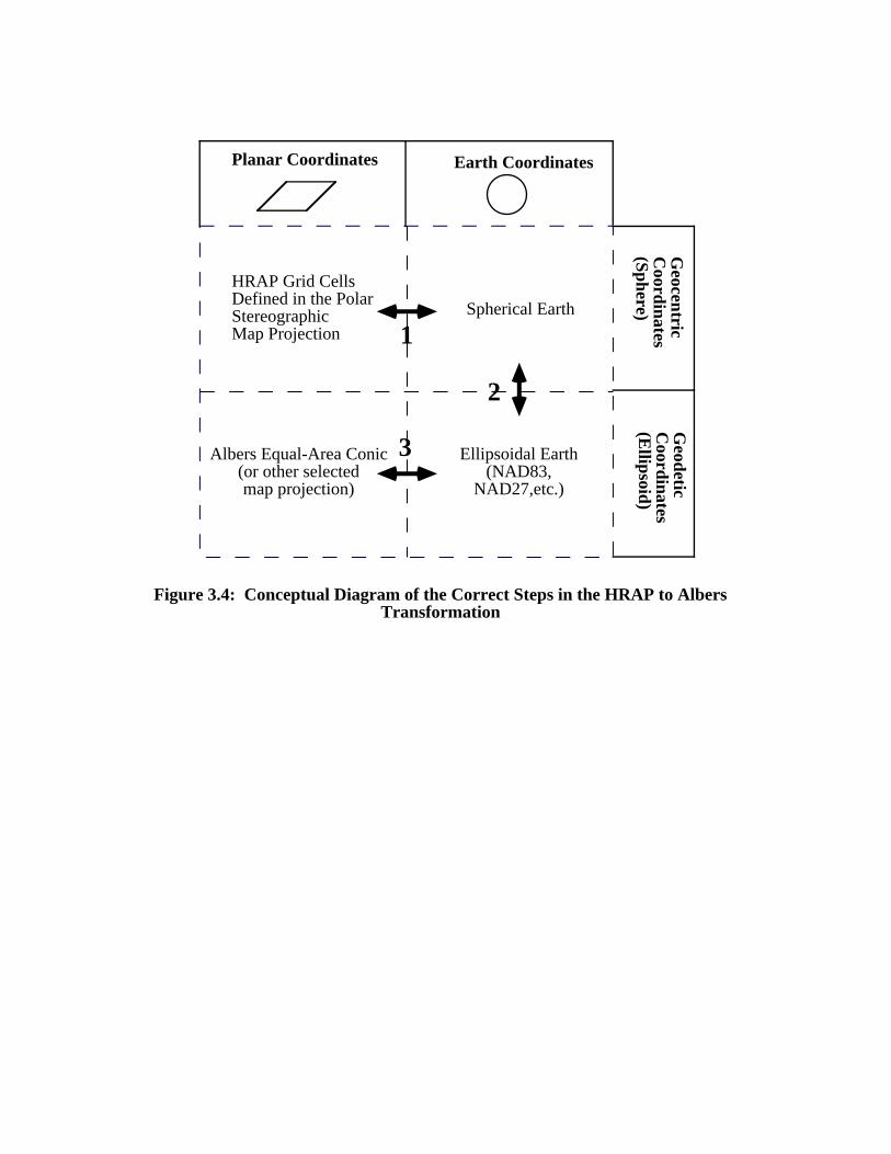
Planar Coordinates Earth Coordinates

HRAP Grid CellsDefined in the PolarStereographicMap Projection

Albers Equal-Area Conic(or other selectedmap projection)

Spherical Earth

Ellipsoidal Earth(NAD83,

NAD27,etc.)

1

2

3

Geocentric

Coordinates

(Sphere)

Geodetic

Coordinates

(Ellipsoid)

Figure 3.4: Conceptual Diagram of the Correct Steps in the HRAP to AlbersTransformation

55

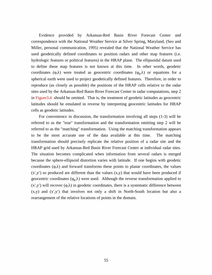
Evidence provided by Arkansas-Red Basin River Forecast Center and

correspondence with the National Weather Service at Silver Spring, Maryland, (Seo and

Miller, personal communication, 1995) revealed that the National Weather Service has

used geodetically defined coordinates to position radars and other map features (i.e.

hydrologic features or political features) in the HRAP plane. The ellipsoidal datum used

to define these map features is not known at this time. In other words, geodetic

coordinates (φ,λ) were treated as geocentric coordinates (φg,λ) or equations for a

spherical earth were used to project geodetically defined features. Therefore, in order to

reproduce (as closely as possible) the positions of the HRAP cells relative to the radar

sites used by the Arkansas-Red Basin River Forecast Center in radar computations, step 2

in Figure3.4 should be omitted. That is, the treatment of geodetic latitudes as geocentric

latitudes should be emulated in reverse by interpreting geocentric latitudes for HRAP

cells as geodetic latitudes.

For convenience in discussion, the transformation involving all steps (1-3) will be

referred to as the "true" transformation and the transformation omitting step 2 will be

referred to as the "matching" transformation. Using the matching transformation appears

to be the most accurate use of the data available at this time. The matching

transformation should precisely replicate the relative position of a radar site and the

HRAP grid used by Arkansas-Red Basin River Forecast Center at individual radar sites.

The situation becomes complicated when information from several radars is merged

because the sphere-ellipsoid distortion varies with latitude. If one begins with geodetic

coordinates (φ,λ) and forward transforms these points to planar coordinates, the values

(x′,y′) so produced are different than the values (x,y) that would have been produced if

geocentric coordinates (φg,λ) were used. Although the reverse transformation applied to

(x′,y′) will recover (φ,λ) in geodetic coordinates, there is a systematic difference between

(x,y) and (x′,y′) that involves not only a shift in North-South location but also a

rearrangement of the relative locations of points in the domain.

56

3.4 DISTORTIONS INVOLVED WITH USING THE HRAP COORDINATE

SYSTEM

It is difficult for us to assess the magnitude of radar mapping errors without more

knowledge about how distances traced out by a NEXRAD radar beam are converted to

distances in the HRAP plane. It is also recognized that discussion of errors in this section

is strictly limited to distortion due to map transformations without considering other

errors, such as beam refraction, associated with radar detection of rainfall — other errors

may be considerably larger than map transformation distortions (Seo and Miller, personal

communication, 1995).

There are two types of distortions inherent in the mapping of NEXRAD products in

the HRAP plane and using a spherical transformation on ellipsoidal coordinates: (1)

variation of the scale factor (defined below) with latitude; (2) distortion of the scale

factor because of the spherical transformation applied to ellipsoidal coordinates.

3.4.1 Scale Factor

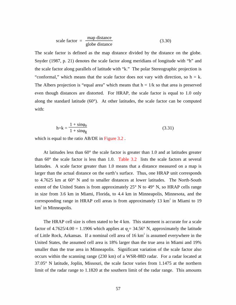
When a map is produced, the dimensions on the earth’s surface are first reduced to

dimensions on a globe in proportion to the map scale, where

map scale = globe distance

earth distance(3.29)

For example, a map scale of 1:100,000 means that 1 cm on the globe corresponds to

100,000 or 1 km on the earth. For HRAP, the map scale is 1 unit = 4.7625 km. The area

on the earth’s surface that an HRAP cell represents varies with latitude. In the HRAP

image plane, all HRAP cells are square and have a side length equal to one unit. When

HRAP cell coordinates are converted to polar Stereographic coordinates, the cells remain

square in the map plane and the map distance of each cell side is 4.7625 km but this is

not the length of a cell side measured on the globe. When a portion of the globe is

projected onto a flat plane, the distance between two points on the globe is distorted by a

scale factor:

57

scale factor = map distance

globe distance(3.30)

The scale factor is defined as the map distance divided by the distance on the globe.

Snyder (1987, p. 21) denotes the scale factor along meridians of longitude with “h” and

the scale factor along parallels of latitude with “k.” The polar Stereographic projection is

“conformal,” which means that the scale factor does not vary with direction, so h = k.

The Albers projection is “equal area” which means that h = 1/k so that area is preserved

even though distances are distorted. For HRAP, the scale factor is equal to 1.0 only

along the standard latitude (60°). At other latitudes, the scale factor can be computed

with:

h=k = 1 + sinφo

1 + sinφg (3.31)

which is equal to the ratio AB/DE in Figure 3.2 .

At latitudes less than 60° the scale factor is greater than 1.0 and at latitudes greater

than 60° the scale factor is less than 1.0. Table 3.2 lists the scale factors at several

latitudes. A scale factor greater than 1.0 means that a distance measured on a map is

larger than the actual distance on the earth’s surface. Thus, one HRAP unit corresponds

to 4.7625 km at 60° N and to smaller distances at lower latitudes. The North-South

extent of the United States is from approximately 25° N to 49° N, so HRAP cells range

in size from 3.6 km in Miami, Florida, to 4.4 km in Minneapolis, Minnesota, and the

corresponding range in HRAP cell areas is from approximately 13 km2 in Miami to 19

km2 in Minneapolis.

The HRAP cell size is often stated to be 4 km. This statement is accurate for a scale

factor of 4.7625/4.00 = 1.1906 which applies at φg= 34.56° N, approximately the latitude

of Little Rock, Arkansas. If a nominal cell area of 16 km2 is assumed everywhere in the

United States, the assumed cell area is 18% larger than the true area in Miami and 19%

smaller than the true area in Minneapolis. Significant variation of the scale factor also

occurs within the scanning range (230 km) of a WSR-88D radar. For a radar located at

37.05° N latitude, Joplin, Missouri, the scale factor varies from 1.1475 at the northern

limit of the radar range to 1.1820 at the southern limit of the radar range. This amounts

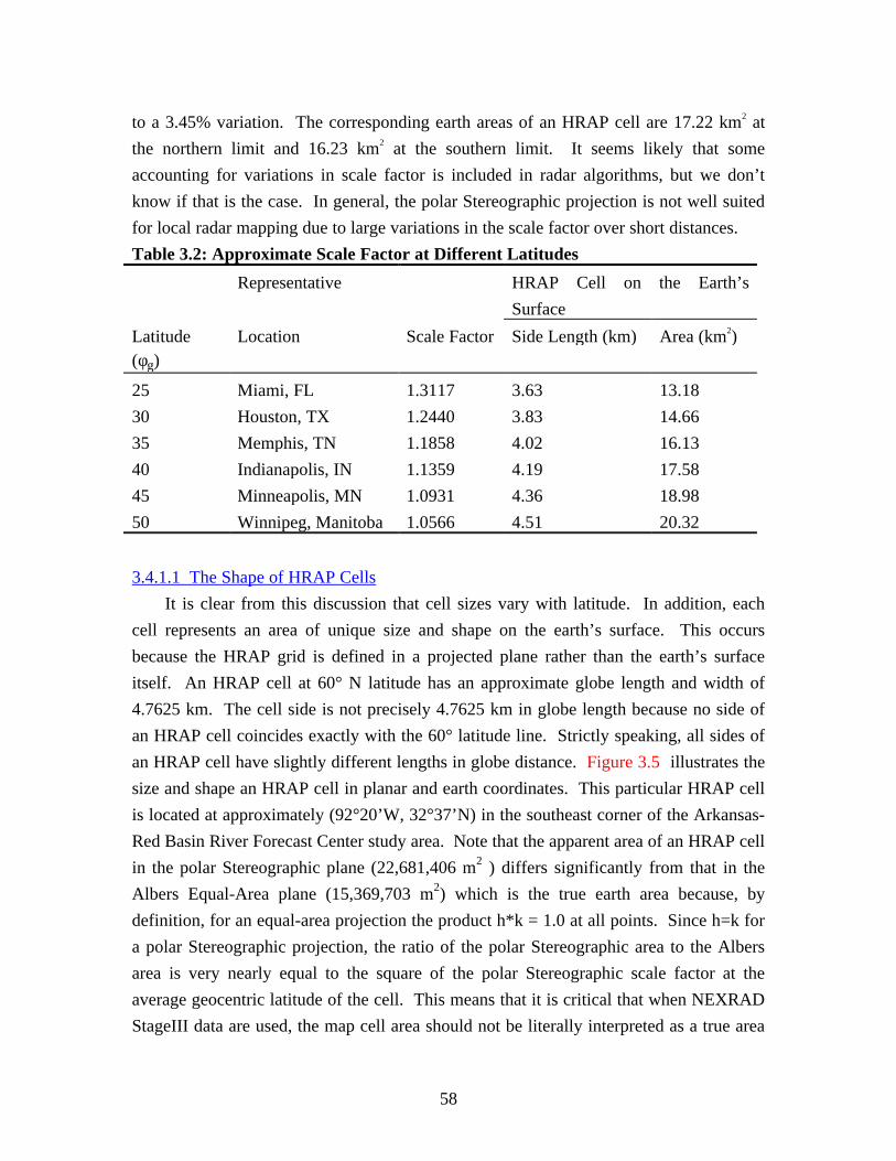
58

to a 3.45% variation. The corresponding earth areas of an HRAP cell are 17.22 km2 at

the northern limit and 16.23 km2 at the southern limit. It seems likely that some

accounting for variations in scale factor is included in radar algorithms, but we don’t

know if that is the case. In general, the polar Stereographic projection is not well suited

for local radar mapping due to large variations in the scale factor over short distances.

Table 3.2: Approximate Scale Factor at Different Latitudes

Representative HRAP Cell on the Earth’s

Surface

Latitude(φg)

Location Scale Factor Side Length (km) Area (km2)

25 Miami, FL 1.3117 3.63 13.18

30 Houston, TX 1.2440 3.83 14.66

35 Memphis, TN 1.1858 4.02 16.13

40 Indianapolis, IN 1.1359 4.19 17.58

45 Minneapolis, MN 1.0931 4.36 18.98

50 Winnipeg, Manitoba 1.0566 4.51 20.32

3.4.1.1 The Shape of HRAP Cells

It is clear from this discussion that cell sizes vary with latitude. In addition, each

cell represents an area of unique size and shape on the earth’s surface. This occurs

because the HRAP grid is defined in a projected plane rather than the earth’s surface

itself. An HRAP cell at 60° N latitude has an approximate globe length and width of

4.7625 km. The cell side is not precisely 4.7625 km in globe length because no side of

an HRAP cell coincides exactly with the 60° latitude line. Strictly speaking, all sides of

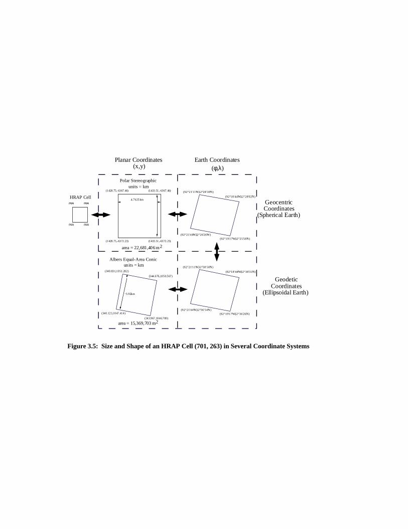
an HRAP cell have slightly different lengths in globe distance. Figure 3.5 illustrates the

size and shape an HRAP cell in planar and earth coordinates. This particular HRAP cell

is located at approximately (92°20’W, 32°37’N) in the southeast corner of the Arkansas-

Red Basin River Forecast Center study area. Note that the apparent area of an HRAP cell

in the polar Stereographic plane (22,681,406 m2 ) differs significantly from that in the

Albers Equal-Area plane (15,369,703 m2) which is the true earth area because, by

definition, for an equal-area projection the product h*k = 1.0 at all points. Since h=k for

a polar Stereographic projection, the ratio of the polar Stereographic area to the Albers

area is very nearly equal to the square of the polar Stereographic scale factor at the

average geocentric latitude of the cell. This means that it is critical that when NEXRAD

StageIII data are used, the map cell area should not be literally interpreted as a true area

(92°21'11" W, 32°38'58" N)

(92°21'44" W, 32°36'54" N)(92°19'17" W, 32°36'26" N)

(92°18'44" W, 32°38'31" N)

(92°21'11" W, 32°28'30" N)

(92°21'44" W , 32°26'26" W)(92°19'17" W, 32°25'58" N)

(92°18'44" W, 32°28'02" N)

(1428.75,-6367.46) (1433.51,-6367.46)

(1428.75,-6372.23) (1433.51,-6372.23)

GeocentricCoordinates

(Spherical Earth)

GeodeticCoordinates

(Ellipsoidal Earth)

(701,264) (702,264)

(701,263) (702,263)

HRAP Cell

Polar Stereographicunits = km

Albers Equal-Area Conicunits = km

area = 15,369,703 m2

area = 22,681,406 m2

Planar Coordinates(x,y)

Earth Coordinates(φ,λ)

4.7625 km

˜3.92 km

(340.123,1047.414)

(340.831,1051.282)

(344.676,1050.567)

(343.967,1046.700)

Figure 3.5: Size and Shape of an HRAP Cell (701, 263) in Several Coordinate Systems

λ �����: λ� ����:

φJ� ����1

φ� ���������1

φ� ���������1

1: 1(

6: 6(

φJ� ����1

� �

��

� �

��

�

��

����

��

��

����

(Denver, CO) (Springfield, IL)

(South of El Paso, TX) (New Orleans, LA)

(Denver, CO)$UHD� ������������P�1:

(Springfield, IL)$UHD� ������������P�1(

(South of El Paso, TX)$UHD� ������������P�6:

(New Orleans, LA)$UHD� ������������P�6(

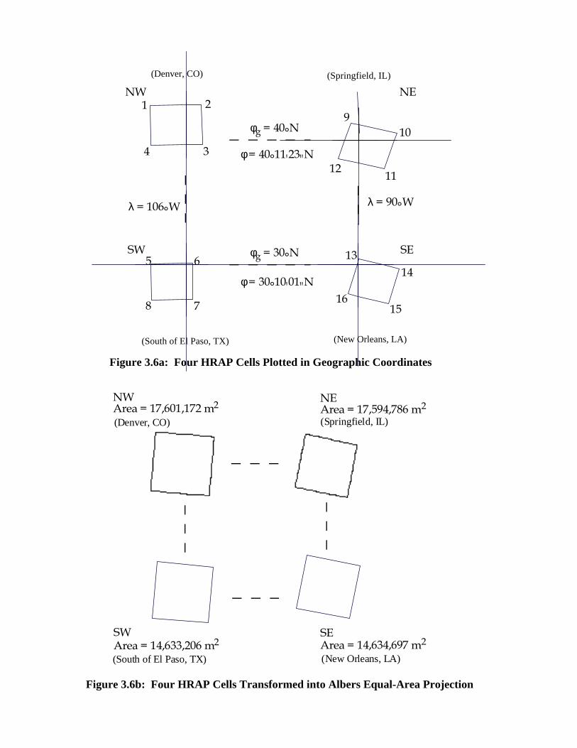
Figure 3.6a: Four HRAP Cells Plotted in Geographic Coordinates

Figure 3.6b: Four HRAP Cells Transformed into Albers Equal-Area Projection

61

on the ground, particularly if a polar Stereographic projection is used. A more reliable

approach is to project the cells into an equal-area projection so that the true earth area is

closely approximated even if each cell still has a unique size and shape.

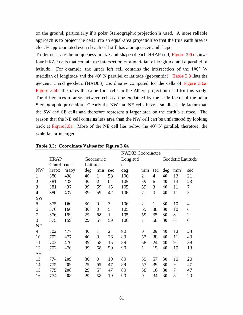
To demonstrate the uniqueness in size and shape of each HRAP cell, Figure 3.6a shows

four HRAP cells that contain the intersection of a meridian of longitude and a parallel of

latitude. For example, the upper left cell contains the intersection of the 106° W

meridian of longitude and the 40° N parallel of latitude (geocentric). Table 3.3 lists the

geocentric and geodetic (NAD83) coordinates computed for the cells of Figure 3.6a.

Figure 3.6b illustrates the same four cells in the Albers projection used for this study.

The differences in areas between cells can be explained by the scale factor of the polar

Stereographic projection. Clearly the NW and NE cells have a smaller scale factor than

the SW and SE cells and therefore represent a larger area on the earth’s surface. The

reason that the NE cell contains less area than the NW cell can be understood by looking

back at Figure3.6a. More of the NE cell lies below the 40° N parallel; therefore, the

scale factor is larger.

Table 3.3: Coordinate Values for Figure 3.6a

NAD83 CoordinatesHRAPCoordinates

GeocentricLatitude

Longitude

Geodetic Latitude

NW hrapx hrapy deg min sec deg min sec deg min sec1 380 438 40 1 58 106 2 4 40 13 212 381 438 40 2 0 105 59 6 40 13 233 381 437 39 59 45 105 59 3 40 11 74 380 437 39 59 42 106 2 0 40 11 5SW5 375 160 30 0 3 106 2 1 30 10 46 376 160 30 0 5 105 59 38 30 10 67 376 159 29 58 1 105 59 35 30 8 28 375 159 29 57 59 106 1 58 30 8 0NE9 702 477 40 1 2 90 0 29 40 12 2410 703 477 40 0 26 89 57 38 40 11 4911 703 476 39 58 15 89 58 24 40 9 3812 702 476 39 58 50 90 1 15 40 10 13SE13 774 209 30 0 19 89 59 57 30 10 2014 775 209 29 59 47 89 57 39 30 9 4715 775 208 29 57 47 89 58 16 30 7 4716 774 208 29 58 19 90 0 34 30 8 20

63

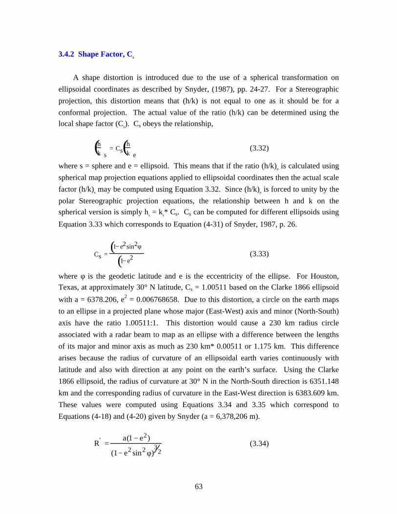
3.4.2 Shape Factor, Cs

A shape distortion is introduced due to the use of a spherical transformation on

ellipsoidal coordinates as described by Snyder, (1987), pp. 24-27. For a Stereographic

projection, this distortion means that (h/k) is not equal to one as it should be for a

conformal projection. The actual value of the ratio (h/k) can be determined using the

local shape factor (Cs). Cs obeys the relationship,

h

k()s

= Csh

k()e

(3.32)

where s = sphere and e = ellipsoid. This means that if the ratio (h/k)e is calculated using

spherical map projection equations applied to ellipsoidal coordinates then the actual scale

factor (h/k)s may be computed using Equation 3.32. Since (h/k)e is forced to unity by the

polar Stereographic projection equations, the relationship between h and k on the

spherical version is simply hs = ks* Cs. Cs can be computed for different ellipsoids using

Equation 3.33 which corresponds to Equation (4-31) of Snyder, 1987, p. 26.

Cs =1−e2sin2φ( )

1−e2( )(3.33)

where φ is the geodetic latitude and e is the eccentricity of the ellipse. For Houston,

Texas, at approximately 30° N latitude, Cs = 1.00511 based on the Clarke 1866 ellipsoid

with a = 6378.206, e2 = 0.006768658. Due to this distortion, a circle on the earth maps

to an ellipse in a projected plane whose major (East-West) axis and minor (North-South)

axis have the ratio 1.00511:1. This distortion would cause a 230 km radius circle

associated with a radar beam to map as an ellipse with a difference between the lengths

of its major and minor axis as much as 230 km* 0.00511 or 1.175 km. This difference

arises because the radius of curvature of an ellipsoidal earth varies continuously with

latitude and also with direction at any point on the earth’s surface. Using the Clarke

1866 ellipsoid, the radius of curvature at 30° N in the North-South direction is 6351.148

km and the corresponding radius of curvature in the East-West direction is 6383.609 km.

These values were computed using Equations 3.34 and 3.35 which correspond to

Equations (4-18) and (4-20) given by Snyder (a = 6,378,206 m).

R' =a(1 − e2)

(1− e2 sin2 φ)3

2(3.34)

64

R’ = radius of curvature in the plane of the meridian

N = a

(1 − e2 sin 2 φ)1

2(3.35)

N = radius of curvature in the plane perpendicular to the meridian and also perpendicular to the tangent

surface

The ratio of the two radii of curvature at 30° N is 6383.609/6351.148 = 1.00511 which is

how the shape factor Cs is determined.

Although the mapping error associated with using a spherical transformation on

ellipsoidal coordinates might seem large (about 0.5% in the example above), it is

important to keep in mind that maps extending over large areas typically introduce larger

variations in the scale factor (Snyder, p.27). For example, with the national Albers

projection used in this study both h and k vary by 0.8% between 30° N and 40° N.

3.5 RECONSIDERING THE MAPPING PROBLEM

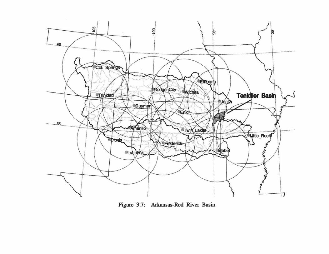
Figure 3.7 shows circles representing the 230 km beam coverage of radars under the

jurisdiction of the the Arkansas-Red Basin River Forecast Center in an Albers Equal-

Area projection. Each circular coverage is a plane, traced out by the radar beam as it

rotates. The angle of elevation of the beam changes during rotation to better sense the

rainfall at different distances from the radar, but essentially each radar coverage is like a

flat map, drawn in the plane of the beam, in which distance and bearing are measured in

polar coordinates relative to the center of rotation, which is the radar location.

There is a class of map projections called azimuthal projections formed by a flat

map tangent to the earth at a given location. The Stereographic projection is one of these

(polar Stereographic means that the projection plane is perpendicular to the polar axis).

If each radar is treated as an individual map and the mosaicing of radar data to form a

composite map is desired, the operation in GIS terms is very straightforward. Each input

“map” is in an azimuthal projection with the projection origin at the radar location and is

forward transformed to a common map reference frame. If the Lambert Azimuthal

Equal-Area projection is used on the input side and Albers Equal-Area on the output

side, the area of radar cells will be preserved in this process. The overlay and

compositing of the precipitation from various radars on the output map is a standard GIS

66

operation. This GIS-based radar data transformation includes all of the required steps in

Figure 3.4 and eliminates the shape factor distortion discussed above.

3.6 VERIFYING CONSISTENCY WITH ARKANSAS-RED BASIN RIVER

FORECAST CENTER HRAP CELLS

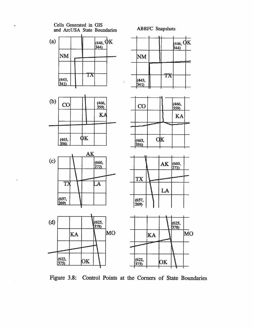
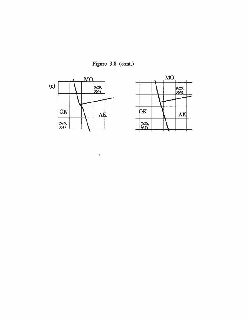
Because of the complications involved with reproducing the HRAP cells in an

ellipsoid-based coordinate system, some checks were made at control points provided by

the Arkansas-Red Basin River Forecast Center to show that the sphere-ellipsoid

transformation (Eqn. 3.8) should not be used for a matching transformation. Norm

Bingham at the Arkansas-Red Basin River Forecast Center provided five “GIF”

snapshots from their software depicting HRAP cells, state boundaries, and a few USGS

gaging stations in the HRAP plane. The five snapshots are in the vicinity of state corners

including the northwest corner of the Texas panhandle, the southeast corner of Colorado,

the northwest corner of Louisiana, the northeast corner of Oklahoma, and the southwest

corner of Missouri. Figure 3.8 (a-e) shows HRAP cells generated in GIS along with

state boundaries from Environmental Systems Research Institute’s ArcUSA CD-ROM in

comparison with Arkansas-Red Basin River Forecast Center snapshots. The state

boundaries from ArcUSA were transformed from geodetic coordinates into the HRAP

coordinate system using Equations 3.17, 3.18, 3.20, and 3.21 for a spherical earth. After

aligning the HRAP cells in our reproduction (first column in Figure 3.8 ) and those

depicted in the ABRFC snapshots (second column in Figure 3.8 ), the distances between

the corners of the state boundaries given by the two sources were approximated. The

largest discrepancy occurred at the northeast corner of Oklahoma and was about 3.3 km

measured in the polar Stereographic plane which corresponds to about 2.8 km on the

earth’s surface. A likely explanation for the discrepancy is that the two sets of state

boundaries came from different sources and are inconsistent which is obvious in Figures

3.8b and e where the two sets of state boundaries clearly have a different shape. The

ArcUSA data is at a relatively large scale, 1:2 million.

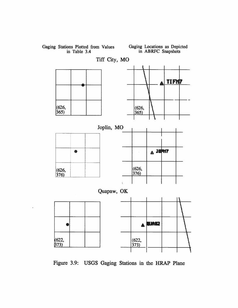
In addition to state boundaries, three USGS gaging stations were identified on the

Arkansas-Red Basin River Forecast Center snapshots, two in Missouri and one in

Oklahoma. The geodetic latitude and longitude for these stations were obtained via

Internet at the address http://h2o.usgs.gov:81/swdata.html. Again, these points were

transformed into HRAP coordinates using Equations 3.17, 3.18, 3.20, and 3.21. These

gaging stations, along with their geographic and HRAP coordinates are listed in

67

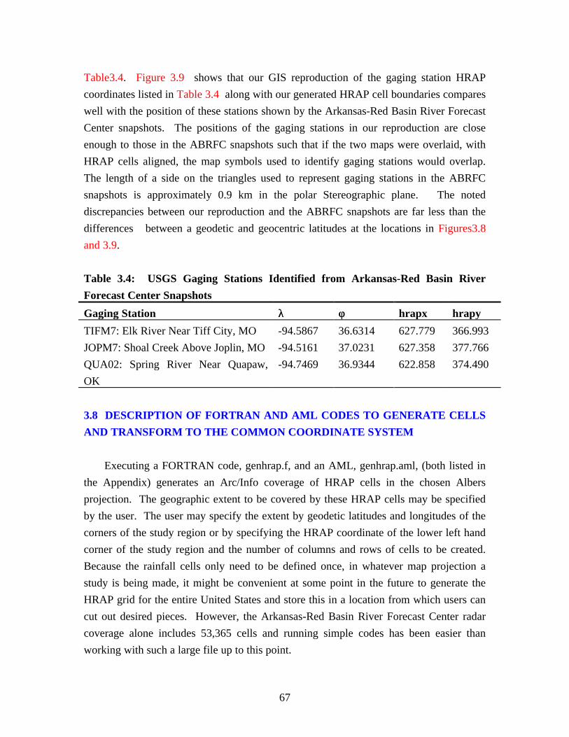
Table3.4. Figure 3.9 shows that our GIS reproduction of the gaging station HRAP

coordinates listed in Table 3.4 along with our generated HRAP cell boundaries compares

well with the position of these stations shown by the Arkansas-Red Basin River Forecast

Center snapshots. The positions of the gaging stations in our reproduction are close

enough to those in the ABRFC snapshots such that if the two maps were overlaid, with

HRAP cells aligned, the map symbols used to identify gaging stations would overlap.

The length of a side on the triangles used to represent gaging stations in the ABRFC

snapshots is approximately 0.9 km in the polar Stereographic plane. The noted

discrepancies between our reproduction and the ABRFC snapshots are far less than the

differences between a geodetic and geocentric latitudes at the locations in Figures3.8

and 3.9.

Table 3.4: USGS Gaging Stations Identified from Arkansas-Red Basin River

Forecast Center Snapshots

Gaging Station λλ φφ hrapx hrapy

TIFM7: Elk River Near Tiff City, MO -94.5867 36.6314 627.779 366.993

JOPM7: Shoal Creek Above Joplin, MO -94.5161 37.0231 627.358 377.766

QUA02: Spring River Near Quapaw,

OK

-94.7469 36.9344 622.858 374.490

3.8 DESCRIPTION OF FORTRAN AND AML CODES TO GENERATE CELLS

AND TRANSFORM TO THE COMMON COORDINATE SYSTEM

Executing a FORTRAN code, genhrap.f, and an AML, genhrap.aml, (both listed in

the Appendix) generates an Arc/Info coverage of HRAP cells in the chosen Albers

projection. The geographic extent to be covered by these HRAP cells may be specified

by the user. The user may specify the extent by geodetic latitudes and longitudes of the

corners of the study region or by specifying the HRAP coordinate of the lower left hand

corner of the study region and the number of columns and rows of cells to be created.

Because the rainfall cells only need to be defined once, in whatever map projection a

study is being made, it might be convenient at some point in the future to generate the

HRAP grid for the entire United States and store this in a location from which users can

cut out desired pieces. However, the Arkansas-Red Basin River Forecast Center radar

coverage alone includes 53,365 cells and running simple codes has been easier than

working with such a large file up to this point.

68

The code for genhrap.f consists of a main program and four subroutines. If the user

chooses to specify the study extent with latitudes and longitudes, the subroutine llinput

computes the corresponding extent of the area in HRAP coordinates. Llinput uses

equations 3.17, 3.18, 3.20, and 3.21 to compute the HRAP coordinate corresponding to

each geographic coordinate specified by the user. From the computed HRAP

coordinates, llinput assigns the minimum hrapx and hrapy coordinates to be the lower left

corner of the study area, computes the approximate number of rows and columns to span

the geographic extent, and returns these values to the main program.

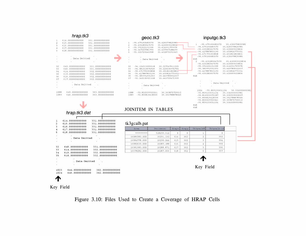
Given the geographic extent of the study area, genhrap.f first writes a file listing the

HRAP coordinates of all corner points to be created beginning with the lower-left corner

of the study area. Coordinates are written for the bottom row moving left to right,

followed by the next row up and so on. This task is performed in the main program and

the file generated is hrap.cod where cod is a user-defined code that is unique for a given

run. For Tenkiller, the file hrap.tk3 was generated. HRAP coordinates from hrap.cod are

converted to geocentric coordinates by the subroutine wll and written to geoc.cod. The

subroutine wll uses the inverses of Equations 3.20 and 3.21, and Equations 3.22, 3.23,

3.24, and 3.28. The subroutine topoly reads the list of corner points from geoc.cod and

creates a file (inputgc.cod) in the appropriate format for generating a polygon coverage.

The last subroutine called by genhrap.f, crdat, writes a file, hrap.cod.dat, used to attach

the correct HRAP-IDs as attributes to the final coverage in Albers. The hrapx and hrapy

coordinates of its lower-left hand corner serve as the ID for an HRAP cell. Precipitation

estimates available on Internet are listed according to the HRAP coordinates of a cell’s

lower-left hand corner; therefore, the HRAP-IDs are the only link between the

geographic position of a cell and a precipitation depth obtained from Arkansas-Red Basin

River Forecast Center.

Given the files inputgc.cod and hrap.cod.dat, genhrap.aml generates a polygon coverage

called codgeocc, projects this coverage into the chosen projection producing

codgeoccalb, creates an INFO data file (hrapxy.dat) and adds data from hrap.cod.dat to

this file, and joins the newly created INFO file to the PAT of codgeoccalb. The file

inputgc.cod is set up so that the polygons in geocentric coordinates that are created from

this file are numbered from left to right starting with the bottom row followed by the

next row up and so on. The numbering system is important because this is the key to

joining the HRAP-IDs to the correct polygons. These polygon numbers get stored in the

field CODGEOCCALB-ID of codgeoccalb.pat. The values in CODGEOCCALB-ID

69

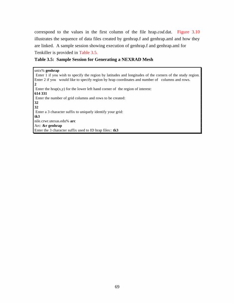
correspond to the values in the first column of the file hrap.cod.dat. Figure 3.10

illustrates the sequence of data files created by genhrap.f and genhrap.aml and how they

are linked. A sample session showing execution of genhrap.f and genhrap.aml for

Tenkiller is provided in Table 3.5.

Table 3.5: Sample Session for Generating a NEXRAD Mesh

unix% genhrap Enter 1 if you wish to specify the region by latitudes and longitudes of the corners of the study region.Enter 2 if you would like to specify region by hrap coordinates and number of columns and rows.2 Enter the hrap(x,y) for the lower left hand corner of the region of interest:614 331 Enter the number of grid columns and rows to be created:3232 Enter a 3 character suffix to uniquely identify your grid:tk3nile.crwr.utexas.edu% arcArc: &r genhrapEnter the 3 character suffix used to ID hrap files:: tk3