An Early Performance Evaluation of the NEXRAD Dual

An Early Performance Evaluation of the NEXRAD Dual-Polarization Radar RainfallEstimates for Urban Flood Applications

LUCIANA K. CUNHA

Department of Civil and Environmental Engineering, Princeton University, Princeton, New Jersey, and Willis Research

Network, London, United Kingdom

JAMES A. SMITH AND MARY LYNN BAECK

Department of Civil and Environmental Engineering, Princeton University, Princeton, New Jersey

WITOLD F. KRAJEWSKI

IIHR—Hydroscience and Engineering, The University of Iowa, Iowa City, Iowa

(Manuscript received 9 April 2013, in final form 24 July 2013)

ABSTRACT

Dual-polarization radars are expected to provide better rainfall estimates than single-polarization radars

because of their ability to characterize hydrometeor type. The goal of this study is to evaluate single- and dual-

polarization radar rainfall fields based on two overlapping radars (Kansas City, Missouri, and Topeka,

Kansas) and a dense rain gauge network in Kansas City. The study area is located at different distances from

the two radars (23–72 km for Kansas City and 104–157km for Topeka), allowing for the investigation of radar

range effects. The temporal and spatial scales of radar rainfall uncertainty based on three significant rainfall

events are also examined. It is concluded that the improvements in rainfall estimation achieved by polari-

metric radars are not consistent for all events or radars. The nature of the improvement depends funda-

mentally on range-dependent sampling of the vertical structure of the storms and hydrometeor types. While

polarimetric algorithms reduce range effects, they are not able to completely resolve issues associated with

range-dependent sampling. Radar rainfall error is demonstrated to decrease as temporal and spatial scales

increase. However, errors in the estimation of total storm accumulations based on polarimetric radars remain

significant (up to 25%) for scales of approximately 650 km2.

1. Introduction

Weather radars have been successfully used for many

years to monitor rainfall and extreme weather events. In

the United States, the first Weather Surveillance Radar-

1988 Doppler (WSR-88D) was installed in 1992, and

since then 159 single-polarization S-band radars (SPRs)

have been deployed. These instruments efficiently de-

tect the structure and evolution of storms and provide

quantitative precipitation estimates (QPEs). There are,

however, large uncertainties in these QPEs (Wilson and

Brandes 1979; Fabry et al. 1992; Baeck and Smith 1998;

Smith et al. 1996; Germann et al. 2006; Szturc et al.

2008; Villarini andKrajewski 2009). These uncertainties

limit the use of SPR QPEs as input to flood simulation

models, especially for urban basins with rapid responses

to short-term rainfall rates (e.g., Carpenter and Geor-

gakakos 2004; Javier et al. 2007; Smith et al. 2007;

Schr€oter et al. 2011; Cunha et al. 2012).

One of the major sources of uncertainty in SPR rainfall

estimates is the lack of a unique relationship between

reflectivity, measured by the radar, and rainfall rate. For

SPR QPEs, measurements of reflectivity are converted

into rainfall rate (mmh21) by a power-law relationship

(Z 5 aRb) for which parameters are empirically esti-

mated. Since the parameters of this relationship depend

on the raindrop size distribution, which varies between

and within storms, there is no unique Z–R relationship

that can satisfy all meteorological phenomena. Other

factors that lead to inaccuracies in radar-derived rainfall

estimates include bright bands (maximums in the radar

Corresponding author address: Luciana Cunha, Department

of Civil and Environmental Engineering, Princeton University,

E-208, Engineering Quad, Princeton, NJ 08544-0001.

E-mail: [email protected]

1478 WEATHER AND FORECAST ING VOLUME 28

DOI: 10.1175/WAF-D-13-00046.1

� 2013 American Meteorological Society

mailto:[email protected]

reflectivity caused by melting snow), incomplete beam

filling, calibration errors, attenuation, anomalous prop-

agation (AP), ground clutter, and the sampling strategy

used by the radar (e.g., Austin 1987; Fo et al. 1998;

Villarini and Krajewski 2009).

Upgrade of the Next Generation Weather Radar

(NEXRAD) network to dual-polarization capabilities

began in 2011. DPRs have the potential tomitigate some

of the uncertainties common to SPRs, since they are able

to discriminate between hydrometeors and other aerial

targets, and to better characterize the hydrometeor type,

as well as the raindrop size distribution illuminated by

the radar beam. SPR provides only measurements of

horizontal reflectivity, and DPR provides both vertical

and horizontal polarization measurements, which are

used to estimate differential reflectivity, differential phase

shift, and the copolar correlation coefficient [see Straka

et al. (2000) for definitions]. These additional variables

are used to improve the QPEs. Previous studies have

demonstrated the ability of DPRs to classify hydrome-

teor types (HTs), to identify the melting layer position

(Straka et al. 2000; Heinselman and Ryzhkov 2006;

Giangrande et al. 2008; Park et al. 2009), and to improve

rainfall estimation (Chandrasekar et al. 1990; Ryzhkov

et al. 2005b; Vulpiani and Giangrande 2009).

To make the best use of these instruments, we need

to fully understand the benefits they provide for QPEs

under different meteorological conditions. This is es-

pecially true for applications to urban flooding for which

high temporal and spatial resolutions, as well as accurate

rainfall estimates, are required (Krajewski and Smith

2002; Smith et al. 2002; Einfalt et al. 2004; Wright et al.

2012). In this study we evaluate SPR and operational

DPRQPEproducts collected by theKansasCity,Missouri

(KEAX), and Topeka, Kansas (KTWX), radars over the

Kansas City metropolitan region. We use Hydro-

NEXRAD to estimate SPR QPEs, while DPR QPEs

were obtained from the instantaneous precipitation rate

(IPR) product of the operational NEXRAD algorithms

and provided by the National Oceanic and Atmospheric

Administration (NOAA). Both radars overlap an area

with a very dense network of rain gauges. Our goal is to

better understandQPE improvements achieved byDPRs,

and how they can improve flood prediction across mul-

tiple scales.

We present an error analysis of QPEs by comparing

the different radar rainfall products with rain gauge

data. We evaluate possible causes of errors in SPR and

DPR QPEs and assess how QPE uncertainties vary

across a range of temporal and spatial scales. Our focus

is on urban flooding, and our evaluation is for basins with

drainage areas varying from approximately 1 to 650 km2

in the Kansas City area.

This works centers on the following questions: Are

rainfall estimates based on DPRs (consistently) better

than rainfall estimates based on SPRs? If not, in which

situations are they better or worse?What is the effect of

range on radar rainfall estimation based on DPRs and

SPRs? Do DPRs provide better estimates of hydrolog-

ically relevant rainfall properties that lead to improved

prediction of flash floods?

In the following section, we present the study area and

experimental data. In section 3, we present the analysis

methods applied in this study. In section 4, we examine

the main results; and in section 5, we discuss our con-

clusions and recommendations for future research.

2. Study area, data, and methods

In this study we compare rainfall fields obtained by

SPRs and DPRs with ground reference data obtained

from a dense rain gauge network in the Kansas City

metropolitan area. We analyze radar rainfall estimates

for three rainfall events that occurred on 19–20 March

2012, 6–7 May 2012, and 31 August–1 September 2012.

Each of the storms occurred after the implementation of

theDPR upgrades to theKEAX (10 February 2012) and

KTWX (30 January 2012) WSR-88Ds. The three storms

exhibited very different characteristics in terms of the

spatial variability of rainfall over the study region, the

magnitudes of the rainfall rate, and the distribution of

hydrometeor types.Wewill describe these differences in

the results session.

a. Rain gauge network

The city of Overland Park and Johnson County,

Kansas, maintain a dense rain gauge network with the

goal of mitigating urban floods. The network collects

rainfall data in near–real time with high temporal reso-

lution (less than 5min) and makes the data freely avail-

able (www.stormwatch.com). The network includes 136

tipping-bucket rain gauges that were operational for the

year 2012; most of the gauges are High Sierra model

2400 gauges (M. Ross 2012, personal communication).

The bucket volume is 1mm and the collected data are

transmitted to the base server in near–real time. While

the bucket size is too coarse for detailed studies of rainfall

rate variability (see Habib et al. 2001), it is deemed ad-

equate for high-intensity and accumulation events that

produce flash floods.

We collected raw data in breakpoint format (times of

1-mm tips) and estimated 15-min rain rates using the tip

interpolation method. Ciach (2003) demonstrated the

advantage of the tip interpolation method compared

to the traditional tip-counting method, especially for

shorter time scales. Even though we use gauge-based

DECEMBER 2013 CUNHA ET AL . 1479

http://www.stormwatch.com

estimates as ground reference, we recognize that tipping-

bucket rain gauge data are subject to systematic and ran-

dom instrumental errors (Zawadzki 1975; Austin 1987;

Habib et al. 2001; Lanza and Stagi 2008).

The accuracy of the gauge versus radar comparisons is

limited by the space–time sampling differences of both

instruments. While tipping buckets sample areas on the

order of 1021m2, radar samples areas of approximately

1 3 106m2. The severity of the effect depends on the

spatial variability of rainfall at a given temporal scale.

Due to the small sample of storms available for this

study, we did not pursue the error variance and co-

variance separation method (Ciach and Krajewski 1999;

Mandapaka et al. 2009) that ‘‘isolate’’ errors due to

sampling scale differences. Nevertheless, the radar versus

gauge comparison does provide diagnostic information

pertinent to our goal of comparing SPR and DPR pre-

cipitation estimates. The scale problem is especially rel-

evant in the comparison of 15-min gauge and radar rain

rates, but it isminimized aswe aggregate the observations

in space or time (Ciach and Krajewski 1999; Seo and

Krajewski 2010; Seo and Krajewski 2011). We examine

both storm total analyses (aggregation in time) and basin-

scale error analyses (aggregation in space).

b. Radar rainfall data

In this study we developed SPR and DPR rainfall

fields over an area of approximately 3600 km2 (60 km by

60 km centered) around Kansas City, using observations

from both the KEAX and KTBW radars. The distance

from the KEAX radar to the rain gauges in the Kansas

City network ranges from 23 to 72 km, while the distance

from the KTWX radar ranges from 104 to 157 km. The

difference in distance from both radars to the study area

allows us to investigate the effects of range on QPE

uncertainty. Range effects on radar rainfall estimation

were previously demonstrated by Smith et al. (1996), Fo

et al. (1998), Fulton et al. (1998), and Krajewski et al.

(2011b).

Figure 1a shows the locations of the two radars and

their distances to the study area, Fig. 1b presents a map

with the rain gauge locations, and Fig. 1c illustrates a

vertical profile where we indicate the radar beam ge-

ometry and height over the study area for both radars for

the lowest elevation angle. Range effects are caused

mainly by an increase in the radar beam height and radar

echo vertical structure heterogeneity with range. De-

pending on the range, the radar beam might partly in-

tercept the melting layer or even completely overshoot

precipitation.

For both radars we will compare rainfall fields that are

based on the SPR-only and DPR NEXRAD measure-

ments. Herein, we refer to KEAX-SPR and KTWX-SPR

for single-polarization (conventional NEXRAD sys-

tem) data and KEAX-DPR and KTWX-DPR for dual-

polarimetric data.

For the generation of the 15-min SPR NEXRAD

rainfall fields we collected level II data from the Na-

tional Climatic Data Center (NCDC) for the two radars.

We used theHydro-NEXRAD radar-rainfall estimation

algorithms to convert reflectivity into 15-min rainfall

accumulation fields at 1-km horizontal resolution. Hydro-

NEXRAD capabilities and the procedures used to

generate rainfall products are described in Krajewski

et al. (2011a) and Krajewski et al. (2007). The prepro-

cessing rain-rate algorithm converts reflectivity from

the lowest elevation angle scan to rainfall rate using

the standard Z–R relationship for convective events

(Fulton et al. 1998). The user can specify the power-law

empirical relationship between the reflectivity and

rainfall intensity. For this study we applied the ‘‘quick

look’’ algorithm (refer to Krajewski et al. 2011a), which

provides standard parameters (Z5 300R1:4) to gener-

ate 15-min and 1 km3 1 km accumulated rainfall maps.

We applied a quality control algorithm that performs

anomalous propagation correction (Steiner and Smith

2002), but omits range correction and advection cor-

rection. Hydro-NEXRAD provides rainfall fields with

a nominal grid resolution of 1 km 3 1 km in the Super

Hydrologic Rainfall Analysis Project (SHRAP) format

based on the HRAP algorithm of Reed and Maidment

(1999). We used standard procedures to reproject the

dataset to geographic coordinates.

In this study, we utilized the operational instan-

taneous precipitation rate (IPR) product to derive the

DPR rainfall fields for both KEAX and KTBW. The

DPR rainfall algorithms (Istok et al. 2009) were devel-

oped in part from the results obtained by the Joint

Polarization Experiment (JPOLE) described by Ryzhkov

et al. (2005b), Heinselman and Ryzhkov (2006), and Park

et al. (2009).

One of the advantages of DPR is the classification of

the hydrometeor type in the sample volume. In addition

to the IPR rainfall fields, we also use the operational

hybrid hydrometeor classification (HHC) fields. For the

initial operational capabilities the NEXRAD agencies

defined the following hydrometeor classes: 1) biological,

2) ground clutter and anomalous propagation, 3) ice

crystal, 4) dry snow, 5) wet snow, 6) light–moderate rain,

7) heavy rain, 8) big drops, 9) graupel, 10) hail (mixed

with rain), and 11) unknown. TheHTs are defined based

on a fuzzy logic method that takes into consideration

measurement uncertainties: lower weights are given to

uncertain measurements in the classification scheme.

Themelting layer (ML) position is usually identified based

on the layer with maximum reflectivity and differential


reflectivity, andminimum correlation coefficient (Brandes

and Ikeda 2004; Giangrande et al. 2008). Based on these

parameters a snow score is estimated and used to define

the melting-layer top and bottom. When the melting

layer cannot be identified by this procedure, the top of

the melting layer is defined at the 08C isotherm and the

bottom is located 500m below the top. The 08C isotherm

is obtained from the Rapid Update Cycle model [see

Benjamin (1989) and Schuur et al. (2011) for details].

Once the height of themelting layer is defined, theHHC

is estimated based on the best–lowest available scan

for each location. The HHC and the melting layer po-

sition determine the rainfall-rate estimation algorithm

(Giangrande andRyzhkov 2008). Note that the different

procedures used to define the melting layer can be

a source of uncertainty on the definition of HHC and

consequently on QPE estimation.

Table 1 presents a summary of the hydrometeor

classes and estimation equations used. These equations

are defined by Giangrande and Ryzhkov (2008) based

on empirical data for Oklahoma. They note that the

parameters for these equations are optimized for the

Oklahoma data and that the validity of the equations

should be tested using data collected under different

climatological conditions.

Differential reflectivity Zdr and reflectivity Z are

used in the case of light, moderate, and heavy rain, and

big drops. In the case of hail below the melting layer,

only DZ is used. For the remaining cases (wet snow,

graupel, hail above the melting layer, dry snow, and ice

crystals), the standard Z–R relationship is used and

a fixed correction is performed depending on the class

(Ryzhkov et al. 2005b). For example, for wet snow the

value calculated by the standard Z–R relationship is

FIG. 1. (a) The 200-km umbrellas of the KEAX and KTWX radars and the basin location. (b) Rain gauge locations

(blue dots) with gray shading denoting different degrees of the Kansas City impervious area (2006). (c) A schematic

vertical profile where the KEAX andKTWX sampling areas (beam geometry and height) above the basin are indicated.


reduced by 40%, and for graupel and hail by 20%. For

dry snow and ice crystals, the Z–R values area increased

by 280%.

Some of the HHC classes are identified only if the

radar beam partly (or completely) overshoots the rain-

fall and intercepts parts of the melting layer. For ex-

ample, ice crystals are observed if the radar beam

completely overshoots the melting layer. Graupel, dry

snow, andwet snow are typically all present when part of

the radar beam is actually sampling the melting layer.

We use these classes to identify the regions in the study

area for which either the KEAX or KTWX radar

overshoots the rainfall. Overshooting is more likely to

happen for KTWX since it is located farther from the

study area.

The IPR fields are in a polar coordinate system and

we used the NOAA toolkit to transform the data to

geographical coordinates, with spatial resolution of ap-

proximately 1 km3 1 km. Both IPR and HHC fields are

provided for each volume scan. In the typical rainfall

mode operation, NEXRAD radars collect a volume

scan every 4–6min. To obtain 15-min time series, we first

interpolated both variables to produce maps with 1-min

time resolution. We then aggregate the 1-min values to

the desired temporal resolution (15, 30, and 60min). For

IPC, we applied linear interpolation, while for HHC we

used the nearest-neighbor interpolation method.

c. Methods

The goal of this paper is to assess improvements in

QPEs obtained by dual-polarization radars and to explore

the potential of applying this dataset to urban hydrology

even when ground data are not available. Therefore, we

evaluate radar rainfall estimates without removing sys-

tematic biases relative to rain gauges. Moreover, this

correction requires long series of data, which are not yet

available for polarimetric radars. For all the analyses

performed in this paper, we calculate the normalized bias

(NB); the standard error (SE), also called root-mean-

square error; and the Pearson correlation coefficient

(CORR), which are defined as follows:

normalized bias,

NB(s)5�D(s,t) 2Dref(s,t)

�Dref(s,t);

standard error,

SE(s) 5

ffiffiffiffiffiffiffiffiffiffiffiffiffiffiffiffiffiffiffiffiffiffiffiffiffiffiffiffiffiffiffiffiffiffiffiffiffiffiffiffiffiffi�[D(s,t)2Dref(s,t)]

2

N

s; and

Pearson correlation coefficient,

CORR(s) 5cov[D(s,t),Dref(s,t)]

sD(s) 3sDref(s)

5E[D(s,t)2E[D(s,t)]]3E[Dref(s,t) 2E[Dref(s,t)]]

sD(s) 3sDref(s)

.

CORR measures the degree of linear association be-

tween the radar and gauge measurements. The quanti-

ties E[X] and sX are the expected value and the

standard deviation of X, respectively. NB and CORR

are dimensionless, and SE is in millimeters or millime-

ters per hour. The index s refers to a specific spatial

domain that can be a gauge location or a subbasins, and t

to the time intervals. NB is a measure of the overall bias

(B), which represents systematic average deviations of

radar estimates with respect to the rain gauge estimation

over the spatial domain of interest (gauge location or

subbasin). SE is a measure of dispersion and indicates how

TABLE 1. Hydrometeor types and radar rainfall estimation equations.

Symbol Hydrometeor type Position in relation to the ML* Rain equation

GC Ground clutter–anomalous propagation CB, PB, PA, MW R 5 0

BI Biological CB, PB, MW, PA R 5 0

RA Light–moderate rain CB or PB R(Z, Zdr)

HR Heavy rain CB or PB R(Z, Zdr)

BD Big drops CB, PB, MW, PA R(Z, Zdr)

HA Hail mixed with rain CB, PB, MW, PA R(Zdr)

CA 0.8R(Z)

DS Dry snow CB, PB, MW, PA R(Z)

CA 2.8R(Z)

WS Wet snow PB, MW, PA 0.6R(Z)

GR Graupel PB, MW, PA, CA 0.8R(Z)

IC Ice crystal CA 2.8R(Z)

UK Unknown All R(Z)

* CB 5 completely below, PB 5 partly below, MW 5 mostly within, PA 5 partly above, and CA 5 completely above.


radar measurements differ from their expected value

(gauge estimation). Sincewe do not remove themean field

bias, SE accounts for systematic and random errors.

CORR measures the degree of linear association be-

tween the radar and gauge measurements.

Depending on the analyses, the variables D and Dref

represent total storm accumulations (mm) or 15-min

rain-rate values (mmh21) calculated based on different

rainfall datasets (gauge, SPR, or DPR) estimated over

a point/pixel or over a certain spatial domain (subbasin).

The Dref refers to the gauge data, and the D to one of

the radar products. For the point analyses, the summa-

tions refers to each ith radar–gauge pair, yielding a

sample size by event equal to the number of sites for total

storm accumulations, and the number of sites times the

number of 15-min intervals for the rain-rate comparisons.

Rainfall is the main input for many hydrological

models; therefore, it is important to understand how

rainfall errors change across scales to be able to decide if

a certain dataset is adequate for hydrological application

(from hillslope to large-scale hydrology), and to better

understand uncertainties on the results of the hydro-

logical models (Seo et al. 2013). Previous studies have

demonstrated that radar rainfall estimation errors de-

crease with averaging in space and time (e.g., Knox and

Anagnostou 2009; Seo and Krajewski 2010). This is ex-

pected since averaging a large number of observations

reduces random uncertainties. This is relevant for the

hydrological community, since it means that even if

errors are large for small scales (e.g., 15min in time,

1 km3 1 km in space), there should be a scale for which

errors are in an acceptable range for flood applications.

In this study, we aggregate the information in time

(15–180min) and in space (0.02–650 km2) and calculate

statistical measures described in the previous sections

(NB, SD, and CORR). Because our focus is on pro-

viding information about radar rainfall error scaling in

a hydrologic context, we aggregate the information in

space using basin boundaries, which are natural spatial

domains in hydrology. We use the river networks anal-

ysis tool CUENCAS [see description in Mantilla and

Gupta (2005) and Cunha et al. (2011)] to automatically

extract the river network and the basin boundaries

based on the U.S. Geological Survey’s (USGS) National

Elevation Dataset (NED) 30-m Digital Elevation Map

(DEM; Gesch et al. 2009). We interpolate 15-min rain

gauge data using the inverse-distance-weighting method

to generate spatially continuous rainfall maps with the

same resolution as the radar maps. The interpolated

datasets are used as reference to evaluate radar rainfall

estimates. Due to the high density of gauges (see Fig.

1b), the interpolated maps provide accurate represen-

tation of the rainfall spatial variability in the basin. We

calculate statistical measures and hydrologic parameters

that are relevant for flood simulation, including mean

areal accumulated rainfall and mean areal maximum

rainfall intensity, for each of the nested subbasins, rang-

ing in scale from 0.01 to 650km2. We estimate the mean

areal rainfall for each basin based on the weighted aver-

age of all radar pixels that are enclosed or intersected by

the basin. The weight is proportional to the area of the

pixel that is contained by the basin. Note that even very

small basins can partially intersect more than one pixel.

3. Results

a. Flood summary and storm totals

The March, May, and September 2012 storm events

exhibit contrasting characteristics in terms of rainfall

distribution over the study region, magnitudes of rainfall

rate, melting-layer position, and HT. In Fig. 2, we il-

lustrate the spatial structure of the storm total radar

rainfall for a 160 km3 120 km domain that contains the

Kansas City study region.

The 6–7 May 2012 storm (Fig. 2) was an organized

thunderstorm system that produced damaging winds

and hail. The storm total rainfall fields exhibit large

spatial variability associated with the structure and evo-

lution of the storm system. In Fig. 2, we present rainfall

fields derived from both the DPR and SPR algorithms

for both the KEAX and KTWX radars. In addition to

the spatial variability in storm total rainfall for each of

the four rainfall fields, there are also striking contrasts

among the four radar rainfall fields. One of the central

questions we want to address is whether the DPR rain-

fall estimates are superior to the SPR rainfall estimates.

Over the Kansas City study region, rain gauge storm

totals varied from 10 to 130mm and peak rainfall in-

tensities reached 150mmh21 at 15-min time resolution.

During this event, the U.S. National Weather Service

issued numerous flood warnings for Johnson, Jackson,

andCassCounties that covered theKansasCity area. The

local news channel (KSHB, channel 41) reported the

occurrence of 1-in. hail in the southeast part of the city.

The 19–20 March 2012 storm was a typical spring ex-

tratropical system that produced moderately heavy

rainfall (Fig. 3a) over time periods of 12–24 h. Over the

course of the event there was a temperature drop of

approximately 128C (218–98C) as a cold front passed

through the region; the melting layer was low over the

entire duration of the storm. The KEAX radar detected

a few periods (approximately 1% of the time, for se-

lected regions) with dry snow, while the measurements

performed by the KTWX radar included ice crystals, dry

snow, wet snow, and graupel. These are hydrometeor


types observed only in the melting layer. The storm total

measured by rain gauges varied from 45 to 70mm over

the Kansas City study area.

The 31 August–1 September storm is typical of fall

extratropical systems that produce high storm total rain-

fall (Fig. 3b) over time periods of 12–24 h. The storm

period was characterized by a cold front that became

stationary over the region. In the beginning of the period,

temperatures dropped from a maximum of 388C to 188Cand then remained constant for the rest of the period. The

event was characterized by low-intensity rainfall that

lasted a long period, resulting in storm totals that varied

from 76 to 222mm over the Kansas City study area.

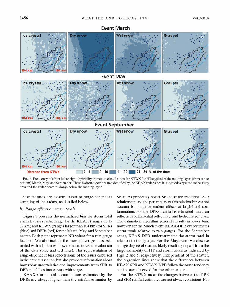
In Fig. 4, we present maps of hydrometeor-type fre-

quency for the KTWX radar for all events. The maps

represent the percentage of the time for which the radar

classified the radar target as ice crystal, dry snow, wet

snow, or graupel during each storm. For theMarch event

among the hydrometeor types are ice crystals, implying

that the radar beam overshoots the precipitation. Dry

snow, wet snow, and graupel are identified when the radar

beam is observing the melting layer. For the March and

Mayevents, themelting layer affects rainfall estimates. For

the September event there is only a brief period of time for

which the bright band affects the rainfall estimates.

In Fig. 5, we present the frequency of HT for the May

event, for light–moderate rain, heavy rain, big drops,

and hail for the KEAX and KTWX radars. The maps

would be identical if both radars were observing the

same layer of the atmosphere and if theHT classification

procedure was error free. The HT observed indicated that

the radar beam captures at least part of the atmosphere

FIG. 2. Storm total accumulation field (mm) derived from (a) KEAX-SPR, (b) KEAX-DPR, (c) KTWX-SPR, and (d) KTWX-DPR

for the May 2012 storm.


below the melting layer. There are several reports of hail

on the ground during theMay event. Both radars detected

hail mainly in the southern part of the study region. The

KTWX radar observed much more hail and more big

drops than did the KEAX radar. This is expected because

the KTWX radar is sampling higher layers of the atmo-

sphere.KEAXdetectedmore heavy rain in the same areas

where KTWX detected more hail.

Figure 6 presents gauge versus radar scatterplots of

storm total rainfall values for the March (green), May

(blue), and September (red) events for SPR (top) and

DPR (bottom) rainfall estimates and for the KEAX

(left) and KTWX (right) radars. Table 2 summarizes

the normalized bias, standard errors, and correlation of

storm total radar rainfall estimates using rain gauge

observations as reference data. We also include the av-

erage (of all gauges) of the percentage of time that each

hydrometeor type was identified by KEAX and KTWX.

The values are calculated for each event and for all

the events together. Note that the KEAX-SPR always

underestimates the storm totals for the March and

September events, and almost always for theMay event.

Close-range biases for SPR are likely caused by a biased

Z–R relationship that compensates for the typical

brightband contamination (Smith et al. 1996); the ab-

sence of brightband contamination in this case leads to

underestimation at close range. For the May event,

KEAX-SPR overestimates storm totals for some of the

gauges. Overestimation occurs for gauges with very low

storm totals in the southwest and in the north of the

basin (less than 20mm) and for regions where hail was

detected. The KEAX-DPR rainfall estimates do not

exhibit systematic underestimation of storm totals. Al-

though smaller in magnitude, bias still exists for the

DPR rainfall estimates. For the March and May storms,

the normalized bias shifts signs from SPRs to DPRs.

KEAX-DPRoverestimates the storm total accumulations.

For the September storm, both KTWX-SPR andKEAX-

DPR underestimate the storm total but KEAX-DPR has

a smaller normalized bias.

KTWX-SPR also underestimates the storm total rain-

fall for the September event, for which no brightband

contamination occurs even at the far ranges. It is likely

that even at these far ranges the effect of biased Z–R re-

lationships can be seen when no brightband contamina-

tion occurs. The opposite effect occurs for the events with

brightband contamination, for which KTWX-SPR over-

estimates rainfall. The absence of a systematic pattern in

normalized bias will be discussed in the next section

where we elaborate upon range effects on storm totals.

The correlation between storm total rainfall from ra-

dar and rain gauge storm total accumulations is larger

for all three events for the KEAX radar (Table 2). For

the KTWX radar, DPR rainfall estimates have a larger

correlation than SPR rainfall estimates for the May and

September storms, but not for the March storm. The

normalized bias is closer to 0 for theMay and September

events for KEAX-DPR rainfall estimates. For KTWX-

DPR, the normalized bias is closer to 0 for the May

storm, but not for the March and September events.

FIG. 3. Storm total accumulation field (mm) derived from KEAX-DPR for the (a) March and (b) September 2012 storms.


These features are closely linked to range-dependent

sampling of the radars, as detailed below.

b. Range effects on storm totals

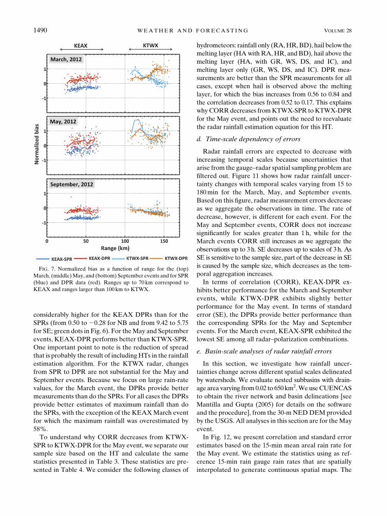
Figure 7 presents the normalized bias for storm total

rainfall versus radar range for the KEAX (ranges up to

72 km) andKTWX (ranges larger than 104 km) for SPRs

(blue) andDPRs (red) for theMarch,May, and September

events. Each point represents NB values for a rain gauge

location. We also include the moving-average lines esti-

mated with a 10-km window to facilitate visual evaluation

of the data (blue and red lines). This representation of

range-dependent bias reflects some of the issues discussed

in the previous section, but also provides information about

how radar uncertainties and improvements from SPR to

DPR rainfall estimates vary with range.

KEAX storm total accumulations estimated by the

DPRs are always higher than the rainfall estimates by

SPRs. As previously noted, SPRs use the traditional Z–R

relationship and the parameters of this relationship cannot

account for range-dependent effects of brightband con-

tamination. For the DPRs, rainfall is estimated based on

reflectivity, differential reflectivity, and hydrometeor class.

The estimation algorithm generally results in lower bias;

however, for theMarch event, KEAX-DPRoverestimates

storm totals relative to rain gauges. For the September

event, KEAX-DPR underestimates the storm total in

relation to the gauges. For the May event we observe

a large degree of scatter, likely resulting in part from the

large variability of HT and storm totals as indicated by

Figs. 2 and 5, respectively. Independent of the scatter,

the regression lines show that the differences between

KEAX-SPR andKEAX-DPR follow the same tendency

as the ones observed for the other events.

For the KTWX radar the changes between the DPR

and SPR rainfall estimates are not always consistent. For

FIG. 4. Frequency of (from left to right) hybrid hydrometeor classification for KTWX for HTs typical of the melting layer: (from top to

bottom)March,May, and September. These hydrometeors are not identified by the KEAX radar since it is located very close to the study

area and the radar beam is always below the melting layer.


the September event, we observe almost no difference

between theKTWX-SPRandKTWX-DPR storm totals.

For theMarch event, the differences betweenKTWX-SPR

and KTWX-DPR are large. KTWX-DPR improved storm

total estimates for ranges up to approximately 130km but

the estimates deteriorated at larger ranges. For the May

storm, we observed significant changes betweenKTWX-

DPR and KTWX-SPR for ranges up to 125 km, some

FIG. 5. Frequency of hybrid hydrometeor classification for (left)

KEAXand (right) KTWX for theMay event: (from top to bottom) light–

moderate rain, heavy rain, big drop rain, and hail.


changes in the 125–140-km range, and almost no changes

for ranges larger than 140 km.

Based on HHC frequency for theMay and September

storms (Table 2), the percentage of light–moderate rain

is not significantly different between KTWX and

KEAX. The main difference is that KTWX detects pe-

riods with graupel, dry snow, wet snow, and ice crystals—

hydrometeors typical of the melting layer—while KEAX

does not detect these HTs. Moreover, KTWX detects hail

more frequently than KEAX. For the March event, sig-

nificant differences are observed between the hydrome-

teor frequency observed by KEAX and by KTWX. For

that event, KTWX almost always samples above the

melting layer, resulting in large errors for KTWX-DPR

rainfall fields. We will discuss this issue in the following

section.

c. Gauge–radar 15-min rain-rate intercomparison

In the previous section we showed that differences

between storm total accumulation based on KTWX-SPR

and KTWX-DPR for the March event are not always

consistent and are range dependent. We observe two

opposing patterns of behavior: for ranges less than 125km,

KTWX-DPR exhibits superior estimation of storm total

rainfall compared to KTWX-SPR, and for ranges greater

than 125km, KTWX-DPR storm total rainfall estimates

areworse than those ofKTWX-SPR. In this section,weuse

the 15-min rain-rate fields and the hydrometeor frequency

time series to investigate the cause of these contrasts.

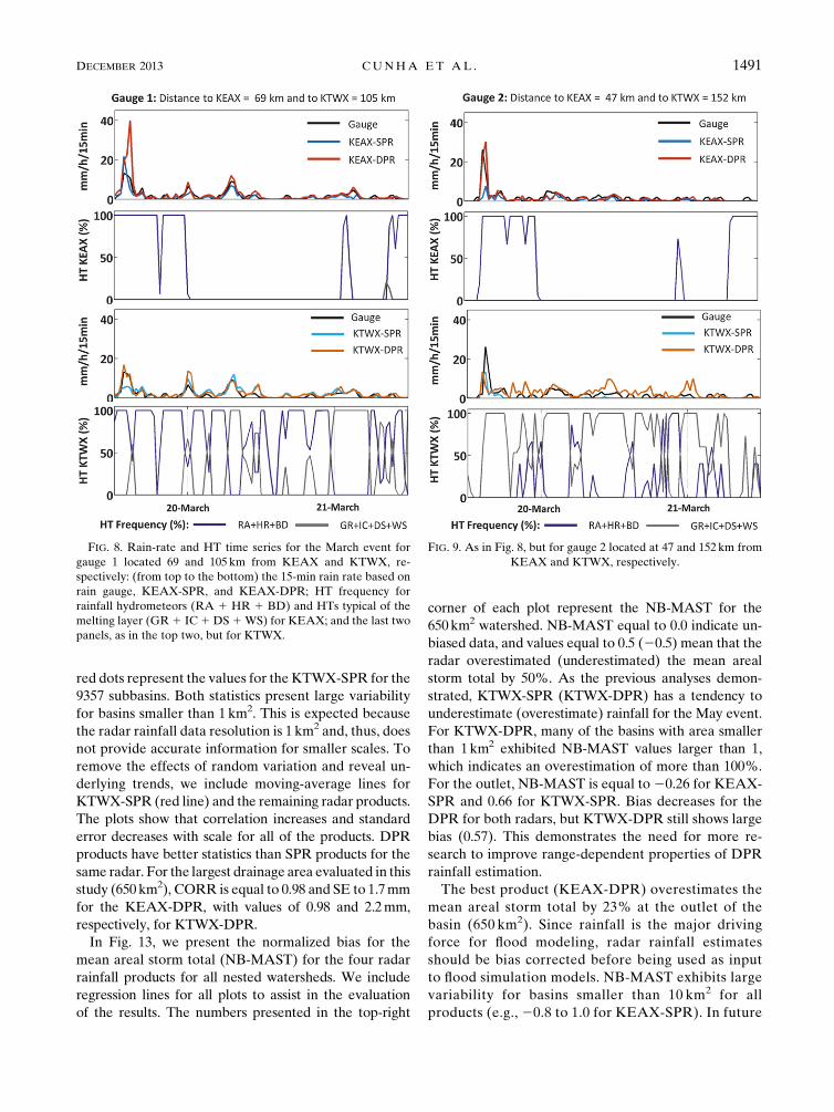
In Figs. 8 and 9, we analyze the time series of rain

rate (gauge, SPR, and DPR) and HT frequency of two

gauges, located at distances of 105 km (gauge 1) and

152 km (gauge 2) from KTWX and 69 km (gauge 1) and

47 km (gauge 2) from KEAX. Figures 8 and 9 present

the 15-min rain-rate time series from the rain gauges,

KTWX-SPR, KEAX-DPR, KTWX-SPR, and KTWX-

DPR, as well as the HT frequencies for KEAX and

KTWX. These two examples demonstrate the lack of

consistency in improvements obtained by DPRs. For

gauge 1 (Fig. 8), KEAX overestimates the first rainfall

peak for both the DPRs and SPRs, with the DPR esti-

mate being worse than that for the SPRs. For KTWX,

the DPRs overestimate and SPRs underestimate the

same peak, with the DPR estimation being considerably

FIG. 6. Scatterplot of gauge vs radar rainfall accumulation for theMarch (green),May (blue),

and September (red) events for the (top) SPR and (bottom)DPR datasets and for (left) KEAX

and (right) KTWX.


better than that of the SPRs. For the remaining time

period, with lighter rain, the KTWX-DPR and KTWX-

SPR rainfall estimates are similar for this gauge. For

gauge 2 (Fig. 9), KEAX-DPR provides a better esti-

mation of the peak than KEAX-SPR, while the KTWX-

SPR and KTWX-DPR estimates of the first peak are

practically the same. However, KTWX-DPR andKTWX-

SPR provide distinct rainfall estimates for the period

with light rainfall. KTWX-SPR did not identify rainfall

for many periods, while KTWX-DPR overestimated

rain. Note that KEAX observes mainly (almost 100%)

hydrometeors associated with rain (RA1HR1BD) for

both gauges, while KTWX observes a mix of rainfall and

melting layer HTs. When analyzing Figs. 8 and 9, we

should remember that tipping-bucket errors are large for

low-intensity rainfall and that this instrument fails to

identify the time that the rainfall started and ended.

Nevertheless, the volume of rainfall should be similar,

which is the case for the gauge 1 estimates at KTWX and

KEAX, but not for gauge 2, with KTWX-DPR over-

estimating and KTWX-SPR underestimating the rainfall.

The difference in bias among theKTWXDPRs and SPRs

for gauge 2 occurs because the DPR algorithm over-

corrects rain rates for frozen hydrometeors, while the

standard Z–R relationship underestimates rain rates

when applied for these hydrometeors.

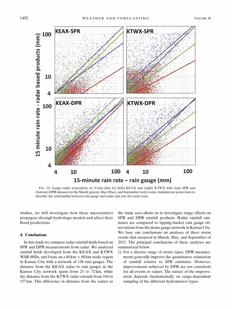
Analyses of 15-min rainfall rates (Fig. 10) indicate

that the DPR rainfall estimates for KEAX are signifi-

cantly better than the SPR rainfall estimates in terms of

both bias and standard error. Figure 10 presents a scat-

terplot of 15-min rain gauge rainfall rate versus 15-min

radar rainfall rate for the radar bin containing the gauge.

The points are color coded by event: green for theMarch

event, blue for theMay event, and red for the September

event. We use power-law functions to describe the dif-

ferences between radar and gauge rainfall as a function

of rain rate (deterministic error) (Ciach et al. 2007;

Villarini et al. 2009). We estimate the parameters of the

power-law function for each rainfall product and event

using the Levenberg–Marquardt algorithm. The improve-

ment in the 15-min radar rainfall estimates for KEAX-

DPR from KTWX-SPR is clear, while KTWX-SPR and

KTWX-DPR show very similar rain-rate estimates.

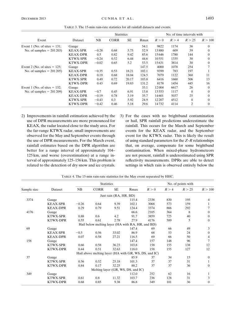
In Table 3, we summarize the 15-min rainfall estima-

tion properties for KEAX and KTWX and for SPR and

DPR measurements. To remove the effects of very low

values (for which gauges are not very accurate), we

calculate CORR, NB, and SE based on the periods for

which gauges observed 15-min rain rates larger than

4mmh21. The correlation improves from SPRs toDPRs

for all events and both radars, except the May storm

for KTWX. For the March storm, NB and SE are

TABLE 2. Storm total statistics for all rainfall datasets and events.

Mar May Sep All

Gauge Avg (mm) 47.40 49.59 126.77

Std dev (mm) 8.75 26.95 30.13

Coefficient of variation 0.18 0.54 0.24

NB KTWX-SPR 20.31 20.26 20.69 20.52

KEAX-DPR 0.31 0.21 20.19 0.00

KTWX-SPR 0.29 0.69 20.30 0.04

KTWX-DPR 0.70 0.56 20.34 0.07

CORR KTWX-SPR 0.77 0.73 0.61 0.46

KEAX-DPR 0.87 0.83 0.81 0.86

KTWX-SPR 0.77 0.85 0.38 0.53

KTWX-DPR 0.22 0.89 0.48 0.43

SE KTWX-SPR 15.95 22.55 91.02 55.39

KEAX-DPR 17.28 21.13 29.65 23.32

KTWX-SPR 21.24 41.18 46.86 38.02

KTWX-DPR 34.87 32.48 50.51 40.23

KEAX HT avg frequency % RA 28.87% 18.69% 54.88% 34.14%

% HR 0.32% 1.10% 0.00% 0.47%

% BD 0.29% 1.67% 0.21% 0.72%

HA 0.01 0.07 0.00 0.03

% GR, DS, WS, and IC 0.04% 0.00% 0.00% 0.01%

% others; no rain 70.47% 78.47% 44.91% 64.62%

KTWX HT avg frequency % RA 5.05% 17.58% 54.85% 25.83%

% HR 0.08% 1.09% 0.00% 0.39%

% BD 0.31% 1.70% 0.22% 0.74%

HA 0.05 0.34 0.00 0.13

% GR, DS, WS, and IC 41.98% 6.30% 0.72% 16.33%

% others; no rain 52.52% 73.00% 44.20% 56.57%


considerably higher for the KEAX DPRs than for the

SPRs (from 0.50 to 20.28 for NB and from 9.42 to 5.75

for SE; green dots in Fig. 6). For theMay and September

events, KEAX-DPR performs better than KTWX-SPR.

One important point to note is the reduction of spread

that is probably the result of includingHTs in the rainfall

estimation algorithm. For the KTWX radar, changes

from SPR to DPR are not substantial for the May and

September events. Because we focus on large rain-rate

values, for the March event, the DPRs provide better

measurements than do the SPRs. For all cases the DPRs

provide better estimates of maximum rainfall than do

the SPRs, with the exception of the KEAXMarch event

for which the maximum rainfall was overestimated by

58%.

To understand why CORR decreases from KTWX-

SPR to KTWX-DPR for theMay event, we separate our

sample size based on the HT and calculate the same

statistics presented in Table 3. These statistics are pre-

sented in Table 4. We consider the following classes of

hydrometeors: rainfall only (RA,HR,BD), hail below the

melting layer (HAwith RA,HR, and BD), hail above the

melting layer (HA, with GR, WS, DS, and IC), and

melting layer only (GR, WS, DS, and IC). DPR mea-

surements are better than the SPR measurements for all

cases, except when hail is observed above the melting

layer, for which the bias increases from 0.56 to 0.84 and

the correlation decreases from 0.52 to 0.17. This explains

why CORRdecreases fromKTWX-SPR toKTWX-DPR

for the May event, and points out the need to reevaluate

the radar rainfall estimation equation for this HT.

d. Time-scale dependency of errors

Radar rainfall errors are expected to decrease with

increasing temporal scales because uncertainties that

arise from the gauge–radar spatial sampling problem are

filtered out. Figure 11 shows how radar rainfall uncer-

tainty changes with temporal scales varying from 15 to

180min for the March, May, and September events.

Based on this figure, radar measurement errors decrease

as we aggregate the observations in time. The rate of

decrease, however, is different for each event. For the

May and September events, CORR does not increase

significantly for scales greater than 1 h, while for the

March events CORR still increases as we aggregate the

observations up to 3h. SE decreases up to scales of 3h. As

SE is sensitive to the sample size, part of the decrease in SE

is caused by the sample size, which decreases as the tem-

poral aggregation increases.

In terms of correlation (CORR), KEAX-DPR ex-

hibits better performance for the March and September

events, while KTWX-DPR exhibits slightly better

performance for the May event. In terms of standard

error (SE), the DPRs provide better performance than

the corresponding SPRs for the May and September

events. For the March event, KEAX-SPR exhibited the

lowest SE among all radar–polarization combinations.

e. Basin-scale analyses of radar rainfall errors

In this section, we investigate how rainfall uncer-

tainties change across different spatial scales delineated

by watersheds. We evaluate nested subbasins with drain-

age area varying from 0.02 to 650km2.WeuseCUENCAS

to obtain the river network and basin delineations [see

Mantilla and Gupta (2005) for details on the software

and the procedure], from the 30-mNEDDEMprovided

by theUSGS.All analyses in this section are for theMay

event.

In Fig. 12, we present correlation and standard error

estimates based on the 15-min mean areal rain rate for

the May event. We estimate the statistics using as ref-

erence 15-min rain gauge rain rates that are spatially

interpolated to generate continuous spatial maps. The

FIG. 7. Normalized bias as a function of range for the (top)

March, (middle)May, and (bottom) September events and for SPR

(blue) and DPR data (red). Ranges up to 70 km correspond to

KEAX and ranges larger than 100km to KTWX.


red dots represent the values for the KTWX-SPR for the

9357 subbasins. Both statistics present large variability

for basins smaller than 1 km2. This is expected because

the radar rainfall data resolution is 1 km2 and, thus, does

not provide accurate information for smaller scales. To

remove the effects of random variation and reveal un-

derlying trends, we include moving-average lines for

KTWX-SPR (red line) and the remaining radar products.

The plots show that correlation increases and standard

error decreases with scale for all of the products. DPR

products have better statistics than SPR products for the

same radar. For the largest drainage area evaluated in this

study (650 km2), CORR is equal to 0.98 and SE to 1.7mm

for the KEAX-DPR, with values of 0.98 and 2.2mm,

respectively, for KTWX-DPR.

In Fig. 13, we present the normalized bias for the

mean areal storm total (NB-MAST) for the four radar

rainfall products for all nested watersheds. We include

regression lines for all plots to assist in the evaluation

of the results. The numbers presented in the top-right

corner of each plot represent the NB-MAST for the

650km2 watershed. NB-MAST equal to 0.0 indicate un-

biased data, and values equal to 0.5 (20.5) mean that the

radar overestimated (underestimated) the mean areal

storm total by 50%. As the previous analyses demon-

strated, KTWX-SPR (KTWX-DPR) has a tendency to

underestimate (overestimate) rainfall for the May event.

For KTWX-DPR, many of the basins with area smaller

than 1km2 exhibited NB-MAST values larger than 1,

which indicates an overestimation of more than 100%.

For the outlet, NB-MAST is equal to20.26 for KEAX-

SPR and 0.66 for KTWX-SPR. Bias decreases for the

DPR for both radars, but KTWX-DPR still shows large

bias (0.57). This demonstrates the need for more re-

search to improve range-dependent properties of DPR

rainfall estimation.

The best product (KEAX-DPR) overestimates the

mean areal storm total by 23% at the outlet of the

basin (650 km2). Since rainfall is the major driving

force for flood modeling, radar rainfall estimates

should be bias corrected before being used as input

to flood simulation models. NB-MAST exhibits large

variability for basins smaller than 10 km2 for all

products (e.g., 20.8 to 1.0 for KEAX-SPR). In future

FIG. 8. Rain-rate and HT time series for the March event for

gauge 1 located 69 and 105 km from KEAX and KTWX, re-

spectively: (from top to the bottom) the 15-min rain rate based on

rain gauge, KEAX-SPR, and KEAX-DPR; HT frequency for

rainfall hydrometeors (RA 1 HR 1 BD) and HTs typical of the

melting layer (GR1 IC1DS1WS) for KEAX; and the last two

panels, as in the top two, but for KTWX.

FIG. 9. As in Fig. 8, but for gauge 2 located at 47 and 152km from

KEAX and KTWX, respectively.


studies, we will investigate how these uncertainties

propagate through hydrologic models and affect their

flood predictions.

4. Conclusions

In this study we compare radar rainfall fields based on

SPR and DPR measurements from radar. We analyzed

rainfall fields developed from the KEAX and KTWX

WSR-88Ds, and focus on a 60 km 3 60 km study region

in Kansas City with a network of 136 rain gauges. The

distance from the KEAX radar to rain gauges in the

Kansas City network spans from 23 to 72 km, while

the distance from the KTWX radar extends from 104 to

157 km. This difference in distance from the radars to

the study area allows us to investigate range effects on

SPR and DPR rainfall products. Radar rainfall esti-

mates are compared to tipping-bucket rain gauge ob-

servations from the dense gauge network inKansas City.

We base our conclusions on analyses of three storm

events that occurred in March, May, and September of

2012. The principal conclusions of these analyses are

summarized below.

1) For a diverse range of storm types, DPR measure-

ments generally improve the quantitative estimation

of rainfall relative to SPR estimates. However,

improvements achieved by DPR are not consistent

for all events or radars. The nature of the improve-

ment depends fundamentally on range-dependent

sampling of the different hydrometeor types.

FIG. 10. Gauge–radar scatterplots of 15-min data for (left) KEAX and (right) KTWX with (top) SPR and

(bottom)DPR datasets for theMarch (green),May (blue), and September (red) events. Included are power laws to

describe the relationship between rain gauge and radar rain rate for each event.


2) Improvements in rainfall estimation achieved by the

use of DPR measurements are more pronounced for

KEAX, the radar located close to the study area. For

the far-range KTWX radar, small improvements are

observed for the May and September events through

the use of DPRmeasurements. For the March event,

rainfall estimates based on the DPR algorithm are

better for a range interval of approximately 104–

125 km, and worse (overestimation) at a range in-

terval of approximately 125–156 km. This problem is

related to the detection of dry snow and ice crystals.

3) For the cases with no brightband contamination

or hail, SPR rainfall predictions underestimate the

rainfall. This occurs for the March and September

events for the KEAX radar, and the September

event for the KTWX radar. This is likely the result

of using standard parameters for theZ–R relationships

that, on average, compensate for some brightband

contamination. When mixed-phase hydrometeors

are not present, rainfall is underestimated using SPR

reflectivity measurements. DPRs are able to detect

settings in which rain is observed entirely below the

TABLE 3. The 15-min rain-rate statistics for all rainfall datasets and events.

Event Dataset

Statistics No. of time intervals with

NB CORR SE Rmax R . 0 R . 4 R . 25 R . 100

Event 1 (No. of sites 5 131;

No. of samples 5 201 203)

Gauge 54.1 9822 1174 36 0

KEAX-SPR 20.28 0.68 5.75 52.9 13 880 609 39 0

KEAX-DPR 0.5 0.82 9.42 85.6 15 646 1780 144 0

KTWX-SPR 20.24 0.52 6.44 44.6 10 551 1335 30 0

KTWX-DPR 20.02 0.65 5.2 53.5 15 631 3814 30 0



Gauge 147.5 4000 1078 254 7

KEAX-SPR 20.35 0.53 18.21 102.1 9399 783 197 1

KEAX-DPR 0.19 0.68 18.04 124.5 7079 1122 360 11

KTWX-SPR 0.49 0.72 20.17 103.8 6416 1660 506 13

KTWX-DPR 0.43 0.69 19.83 131.2 8178 1454 445 16



Gauge 33.1 12 004 6617 26 0

KEAX-SPR 20.7 0.45 6.91 13.8 13 553 1117 0 0

KEAX-DPR 20.19 0.78 3.19 35.7 14 601 5037 25 0

KTWX-SPR 20.43 0.3 5.92 24.9 12 207 4512 0 0

KTWX-DPR 20.42 0.46 5.18 29.6 14 732 4114 2 0

TABLE 4. The 15-min rain-rate statistics for the May event separated by HHC.

Sample size Dataset

Statistics No. of points with

NB CORR SE Rmax R . 0 R . 4 R . 25 R . 100

Just rain (RA, HR, BD)

3374 Gauge 115.4 2338 830 195 4

KEAX-SPR 20.26 0.64 9.39 102.1 3068 573 159 1

KEAX-DPR 0.29 0.79 9.51 124.4 3374 866 292 7

4176 Gauge 66.6 2105 364 8 0

KTWX-SPR 0.88 0.6 4.2 91.7 3859 725 40 0

KTWX-DPR 0.55 0.61 2.78 27.9 4176 589 5 0

Hail below melting layer (HA with RA, HR, and BD)

69 Gauge 147.4 69 66 49 3

KEAX-SPR 20.5 0.56 33.02 86.9 68 53 24 0

KEAX-DPR 0.07 0.58 27.21 116.5 69 66 50 4

158 Gauge 147.4 157 148 96 7

KTWX-SPR 0.66 0.58 36.23 103.8 158 155 138 12

KTWX-DPR 0.44 0.51 32.63 118.0 158 155 127 12

Hail above melting layer (HA with GR, WS, DS, and IC)

37 Gauge 85.9 37 34 15 0

KTWX-SPR 0.56 0.52 25.18 101.3 37 37 31 1

KTWX-DPR 0.84 0.17 32.25 88.2 37 37 36 0

Melting layer (GR, WS, DS, and IC)

349 Gauge 112.0 252 62 16 1

KTWX-SPR 0.61 0.8 11.32 103.7 236 128 31 3

KTWX-DPR 0.68 0.85 9.38 86.8 349 101 36 0


bright band. For these situations, rainfall is estimated

as a function of reflectivity and differential reflectivity.

The addition of differential reflectivity to the rainfall

estimation process has a significant positive impact on

the values estimated for the KEAX radar.

4) DPRs improved the estimation of rainfall when hail

occurred below the top of the melting layer, as was

the case for the Kansas City observations during the

May event. When hail mixed with rain is detected

above the melting layer, as was the case for the KTWX

observations of the May storm, we did not find signif-

icant improvements from DPR measurements.

5) Radar–rain gauge comparisons demonstrate the large

bias for the KEAX-SPR estimates, and the ability of

the DPR algorithm to correct this bias. The normal-

ized bias improved from 20.52 to 0.01. KTWX-SPR

rain rates are characterized by low bias but large

random error, which is slightly improved by the DPR

measurements (decrease in standard error from 3.62

to 3.28).

FIG. 11. Error statistics (radar products compared to gauge rainfall data) with respect to temporal scale for (top to

bottom) the March, May, and September events: (left) CORR and (right) SE.


6) Comparisons of KEAX and KTWX rainfall esti-

mates demonstrate that operational DPR algorithms

reduce range effects, relative to SPR rainfall esti-

mates. In general, improvements are substantial when

the radar detects only raindrops, but inconsistent

otherwise. This might arise from the fact that QPE

algorithms were developed based on data collected

in Oklahoma during the warm season, when snow is

FIG. 12. Error statistics for 15-min rain rates with respect to spatial scale for nested subwatersheds in the study area (May event): (left)

CORR and (right) SE.

FIG. 13. Mean areal storm total normalized biases as a function of spatial scale for nested subwatersheds in the

study area (May event): (top left) KEAX SPR and (top right) DPR; (bottom) as in (top), but for KTWX. The

number at the top right of each plot represents the NB for the 650 km2 watershed.


uncommon in the atmospheric column. Uncer-

tainties in DPR QPEs can also be caused by in-

strument miscalibration (Ryzhkov et al. 2005a). We

cannot further investigate this source of error since we

do not have information about the calibration pro-

cedures performed in KEAX and KTWX, or long

series of data to statistically quantify errorsAdditional

research is needed to address the range-dependent

error structure of DPR rainfall estimates.

7) We demonstrate that the error structure of DPR

QPEs varies considerably from event to event. This is

expected since different radar rainfall algorithms

are used depending on the type of hydrometeor

observed. Empirical models that characterize rainfall

error structure of DPRs (e.g., Villarini et al. 2009)

should explicitly account for range-dependent sam-

pling and the effects of HTs.

8) As we aggregate the observations in time, the corre-

lation increases and the standard error decreases

for all of the rainfall fields. The correlation did not

improve significantly for aggregation times larger than

1h for the May and September events, while for the

March event the correlation continues to increase for

aggregation time up to 3 h (maximum aggregation

time adopted in the study). For the same radar, DPR

rainfall fields provide higher correlations for all events

compared to the SPR fields. We also analyze un-

certainty as a function of spatial scale. We use basin

boundaries to delineate the spatial domain and ag-

gregate the information in space. The analyses dem-

onstrate that for basins up to approximately 20km2

the differences in total accumulations obtained by

gauges and radar exhibit large variability and reach

values of up to 300% for the KTWX-SPR rainfall

fields. Differences for larger basins decrease but are

still significant. For the largest basin (;650 km2) and

the best rainfall estimation, storm total radar rainfall is

overestimated by 23%.This implies that real-time and

retrospective gauge bias correction, as generally ap-

plied to SPR, are likely to be useful for DPRs as well.

This paper is an early attempt to evaluate the system

recently implemented by the NWS to estimate rainfall

based on dual-polarization radars. Future work should

include more events, allowing the use of more rigorous

statistical approaches to quantify radar rainfall errors as

a function of range and hydrometeors types.

Acknowledgments. The authors would like to ac-

knowledge the city of Overland Park Kansas, and spe-

cially Mike Ross, for providing helpful comments about

the rain gauge network. WFK acknowledges support

from the Iowa Flood Center and the Rose and Joseph

Summers endowment. This research was supported

by the Willis Research Network, the National Science

Foundation (Grant CBET-1058027), and the NOAA

Cooperative Institute for Climate Science.

REFERENCES

Austin, P. M., 1987: Relation between measured radar reflectivity

and surface rainfall. Mon. Wea. Rev., 115, 1053–1070.

Baeck,M. L., and J. A. Smith, 1998: Estimation of heavy rainfall by

the WSR-88D. Wea. Forecasting, 13, 416–436.

Benjamin, S. G., 1989: An isentropic mesoa-scale analysis system

and its sensitivity to aircraft and surface observations. Mon.

Wea. Rev., 117, 1586–1603.

Brandes, E. A., and K. Ikeda, 2004: Freezing-level estimation with

polarimetric radar. J. Appl. Meteor., 43, 1541–1553.

Carpenter, T. M., and K. P. Georgakakos, 2004: Impacts of para-

metric and radar rainfall uncertainty on the ensemble stream-

flow simulations of a distributed hydrologic model. J. Hydrol.,

298, 202–221, doi:10.1016/j.jhydrol.2004.03.036.

Chandrasekar, V., V. N. Bringi, N. Balakrishnan, and D. S. Zrni�c,

1990: Error structure of multiparameter radar and surface

measurements of rainfall. Part III: Specific differential phase.

J. Atmos. Oceanic Technol., 7, 621–629.

Ciach, G. J., 2003: Local random errors in tipping-bucket rain gauge

measurements. J. Atmos. Oceanic Technol., 20, 752–759.

——, andW. F. Krajewski, 1999: On the estimation of radar rainfall

error variance. Adv. Water Resour., 22, 585–595, doi:10.1016/

S0309-1708(98)00043-8.

——, ——, and G. Villarini, 2007: Product-error-driven uncer-

tainty model for probabilistic quantitative precipitation esti-

mation with NEXRAD data. J. Hydrometeor., 8, 1325–1347.

Cunha, L. K.,W. F. Krajewski, andR.Mantilla, 2011: A framework

for flood risk assessment under nonstationary conditions or in

the absence of historical data. J. Flood Risk Manage., 4, 3–22.

——, P. V. Mandapaka, W. F. Krajewski, R. Mantilla, and A. A.

Bradley, 2012: Impact of radar-rainfall error structure on es-

timated flood magnitude across scales: An investigation based

on a parsimonious distributed hydrological model. Water Re-

sour. Res., 48, W10515, doi:10.1029/2012WR012138.

Einfalt, T., K. Arnbjerg-Nielsen, C. Golz, N.-E. Jensen,

M. Quirmbach, G. Vaes, and B. Vieux, 2004: Towards a

roadmap for use of radar rainfall data in urban drainage.

J. Hydrol., 299, 186–202.

Fabry, F., G. L. Austin, and D. Tees, 1992: The accuracy of rainfall

estimates by radar as a function of range. Quart. J. Roy. Me-

teor. Soc., 118, 435–453.

Fo,A. J. P., K.C.Crawford, andC. L.Hartzell, 1998: ImprovingWSR-

88D hourly rainfall estimates. Wea. Forecasting, 13, 1016–1028.Fulton, R. A., J. P. Breidenbach, D.-J. Seo, D. A. Miller, and

T. O’Bannon, 1998: The WSR-88D rainfall algorithm. Wea.

Forecasting, 13, 377–395.

Germann, U., G. Galli, M. Boscacci, and M. Bolliger, 2006: Radar

precipitation measurement in a mountainous region. Quart.

J. Roy. Meteor. Soc., 132, 1669–1692.

Gesch, D., G. Evans, J. Mauck, J. Hutchinson, and W. J. Carswell

Jr., 2009. The National Map—Elevation. U.S. Geological

Survey Fact Sheet 2009-3053, 4 pp. [Available online at http://

pubs.usgs.gov/fs/2009/3053/.]

Giangrande, S. E., and A. V. Ryzhkov, 2008: Estimation of rainfall

based on the results of polarimetric echo classification. J. Appl.

Meteor. Climatol., 47, 2445–2460.


http://pubs.usgs.gov/fs/2009/3053/

http://pubs.usgs.gov/fs/2009/3053/

——, J. M. Krause, and A. Ryzhkov, 2008: Automatic designation

of themelting layer with a polarimetric prototype of theWSR-

88D radar. J. Appl. Meteor. Climatol., 47, 1354–1364.

Habib, E., W. F. Krajewski, and A. Kruger, 2001: Sampling errors

of tipping-bucket rain gaugemeasurements. J. Hydrol. Eng., 6,

159–166.

Heinselman, P. L., and A. V. Ryzhkov, 2006: Validation of polar-

imetric hail detection. Wea. Forecasting, 21, 839–850.Istok, M. J., M. Fresch, Z. Jing, and S. Smith, 2009: WSR-88D dual

polarization initial operational capabilities. Preprints, 25th

Conf. on International Interactive Information and Processing

Systems (IIPS) for Meteorology, Oceanography, and Hydrol-

ogy, Phoenix, AZ, Amer.Meteor. Soc., 15.5. [Available online

at https://ams.confex.com/ams/pdfpapers/148927.pdf.]

Javier, J. R. N., J. A. Smith, K. L. Meierdiercks, M. L. Baeck, and

A. J. Miller, 2007: Flash flood forecasting for small urban

watersheds in the Baltimore metropolitan region. Wea. Fore-

casting, 22, 1331–1344.

Knox, R., and E. N. Anagnostou, 2009: Scale interactions in radar

rainfall estimation uncertainty. J. Hydrol. Eng., 14, 944–953.

Krajewski, W. F., and J. A. Smith, 2002: Radar hydrology: Rainfall

estimation. Adv. Water Resour., 25, 1387–1394, doi:10.1016/

S0309-1708(02)00062-3.

——, B.-C. Seo, A. Kruger, P. Domaszczynski, G. Villarini, and

C. Gunyon, 2007: Hydro-NEXRAD radar-rainfall estimation

algorithm development, testing and evaluation. Proc. World

Environmental and Water Resources Congress 2007: Restoring

Our Natural Habitat, Reston, VA, American Society of Civil

Engineers, 9 pp., doi:10.1061/40927(243)279.

——, A. Kruger, J. A. Smith, R. Lawrence, and C. Gunyon, 2011a:

Towards better utilization of NEXRADdata in hydrology: An

overview of Hydro-NEXRAD. J. Hydroinf., 13, 255–266.

——, B. Vignal, B.-C. Seo, and G. Villarini, 2011b: Statistical

model of the range-dependent error in radar-rainfall estimates

due to the vertical profile of reflectivity. J. Hydrol., 402, 306–

316, doi:10.1016/j.jhydrol.2011.03.024.

Lanza, L. G., and L. Stagi, 2008: Certified accuracy of rainfall data

as a standard requirement in scientific investigations. Adv.

Geosci., 16, 43–48.

Mandapaka, P. V., W. F. Krajewski, G. J. Ciach, G. Villarini, and

J. A. Smith, 2009: Estimation of radar-rainfall error spatial

correlation. Adv. Water Resour., 32, 1020–1030, doi:10.1016/

j.advwatres.2008.08.014.

Mantilla, R., and V. K. Gupta, 2005: A GIS numerical framework

to study the process basis of scaling statistics on river net-

works. IEEE Geophys. Remote Sens. Lett., 2, 404–408.

Park, H. S., A. V. Ryzhkov, and D. S. Zrni�c, 2009: The hydrome-

teor classification algorithm for the polarimetric WSR-88D:

Description and application to an MCS.Wea. Forecasting, 24,730–748.

Reed, S. M., and D. R. Maidment, 1999: Coordinate trans-

formations for using NEXRAD data in GIS-based hydrologic

modeling. J. Hydrol. Eng., 4, 174–182.

Ryzhkov, A. V., S. E. Giangrande, V. M. Melnikov, and T. J.

Schuur, 2005a: Calibration issues of dual-polarization radar

measurements. J. Atmos. Oceanic Technol., 22, 1138–1155.——, ——, and T. J. Schuur, 2005b: Rainfall estimation with a po-

larimetric prototype of WSR-88D. J. Appl. Meteor., 44, 502–515.

Schr€oter, K., X. Llort, C. Velasco-Forero, M. Ostrowski, and

D. Sempere-Torres, 2011: Implications of radar rainfall esti-

mates uncertainty on distributed hydrological model pre-

dictions. Atmos. Res., 100, 237–245.Schuur, T. J., H.-S. Park, A. V. Ryzhkov, and H. D. Reeves, 2011:

Classification of precipitation types during transitional winter

weather using the RUC model and polarimetric radar re-

trievals. J. Appl. Meteor. Climatol., 51, 763–779.Seo, B.-C., and W. F. Krajewski, 2010: Scale dependence of radar

rainfall uncertainty: Initial evaluation of NEXRAD’s new

super-resolution data for hydrologic applications. J. Hydro-

meteor., 11, 1191–1198.——, and ——, 2011: Investigation of the scale-dependent vari-

ability of radar-rainfall and rain gauge error correlation. Adv.

Water Resour., 34, 152–163, doi:10.1016/j.advwatres.2010.10.——, L. K. Cunha, and W. F. Krajewski, 2013: Uncertainty in

radar-rainfall composite and its impact on hydrologic pre-

diction for the eastern Iowa flood of 2008. Water Resour. Res.,

49, 2747–2764, doi:10.1002/wrcr.20244.Smith, J. A., D.-J. Seo, M. L. Baeck, and M. D. Hudlow, 1996: An

intercomparison study of NEXRAD precipitation estimates.

Water Resour. Res., 32, 2035–2045.

——, M. L. Baeck, J. E. Morrison, P. L. Sturdevant-Rees,

D. F. Turner-Gillespie, and P. D. Bates, 2002: The regional

hydrology of extreme floods in an urbanizing drainage basin.

J. Hydrometeor., 3, 267–282.——, ——, K. L. Meierdiercks, A. J. Miller, and W. F. Krajewski,

2007: Radar rainfall estimation for flash flood forecasting in

small urban watersheds. Adv. Water Resour., 30, 2087–2097.

Steiner, M., and J. A. Smith, 2002: Use of three-dimensional re-

flectivity structure for automated detection and removal of

nonprecipitating echoes in radar data. J. Atmos. Oceanic

Technol., 19, 673–685.

Straka, J. M., D. S. Zrni�c, and A. V. Ryzhkov, 2000: Bulk hydro-

meteor classification and quantification using polarimetric

radar data: Synthesis of relations. J. Appl. Meteor., 39, 1341–

1372.

Szturc, J., K.O�sr�odka,A. Jurczyk, andL. Jelonek, 2008: Concept of

dealing with uncertainty in radar-based data for hydrological

purpose. Nat. Hazards Earth Syst. Sci., 8, 267–279.

Villarini, G., and W. F. Krajewski, 2009: Review of the different

sources of uncertainty in single polarization radar-based esti-

mates of rainfall. Surv. Geophys., 31, 107–129.

——, ——, G. J. Ciach, and D. L. Zimmerman, 2009: Product-

error-driven generator of probable rainfall conditioned on

WSR-88D precipitation estimates. Water Resour. Res., 45,

W01404, doi:10.1029/2008WR006946.

Vulpiani, G., and S. Giangrande, 2009: Rainfall estimation from

polarimetric S-band radar measurements: Validation of a

neural network approach. J. Appl.Meteor. Climatol., 48, 2022–

2036.

Wilson, J. W., and E. A. Brandes, 1979: Radar measurement of

rainfall—A summary. Bull. Amer. Meteor. Soc., 60, 1048–1058.

Wright, D. B., J. A. Smith, G. Villarini, andM. L. Baeck, 2012: The

hydroclimatology of flash flooding in Atlanta. Water Resour.

Res., 48, W04524, doi:10.1029/2011WR011371.

Zawadzki, I. I., 1975: On radar-raingage comparison. J. Appl.

Meteor., 14, 1430–1436.


https://ams.confex.com/ams/pdfpapers/148927.pdf

Documents

An Early Performance Evaluation of the NEXRAD Dual