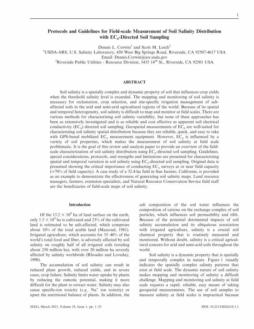
Protocols and Guidelines for Field-scale Measurement of Soil Salinity Distributionwith ECa-Directed Soil Sampling

Dennis L. Corwin1 and Scott M. Lesch2

1USDA-ARS, U.S. Salinity Laboratory, 450 West Big Springs Road, Riverside, CA 92507-4617 USA

Email: Dennis.Corwin@ars.usda.gov2Riverside Public Utilities - Resource Division, 3435 14th St., Riverside, CA 92501 USA

ABSTRACT

Soil salinity is a spatially complex and dynamic property of soil that influences crop yields

when the threshold salinity level is exceeded. The mapping and monitoring of soil salinity is

necessary for reclamation, crop selection, and site-specific irrigation management of salt-

affected soils in the arid and semi-arid agricultural regions of the world. Because of its spatial

and temporal heterogeneity, soil salinity is difficult to map and monitor at field scales. There are

various methods for characterizing soil salinity variability, but none of these approaches has

been as extensively investigated and is as reliable and cost effective as apparent soil electrical

conductivity (ECa) directed soil sampling. Geospatial measurements of ECa are well-suited forcharacterizing soil salinity spatial distribution because they are reliable, quick, and easy to take

with GPS-based mobilized ECa measurement equipment. However, ECa is influenced by a

variety of soil properties, which makes the measurement of soil salinity at field scale

problematic. It is the goal of this review and analysis paper to provide an overview of the field-

scale characterization of soil salinity distribution using ECa-directed soil sampling. Guidelines,

special considerations, protocols, and strengths and limitations are presented for characterizing

spatial and temporal variation in soil salinity using ECa-directed soil sampling. Original data is

presented showing the critical importance of conducting ECa surveys at or near field capacity($70% of field capacity). A case study of a 32.4-ha field in San Jacinto, California, is provided

as an example to demonstrate the effectiveness of generating soil salinity maps. Land resource

managers, farmers, extension specialists, and Natural Resource Conservation Service field staff

are the beneficiaries of field-scale maps of soil salinity.

Introduction

Of the 13.2 3 109 ha of land surface on the earth,

only 1.5 3 109 ha is cultivated and 23% of the cultivated

land is estimated to be salt-affected, which comprises

about 10% of the total arable land (Massoud, 1981).

Irrigated agriculture, which accounts for 35–40% of the

world’s total food and fiber, is adversely affected by soil

salinity on roughly half of all irrigated soils (totaling

about 250 million ha), with over 20 million ha severely

affected by salinity worldwide (Rhoades and Loveday,

1990).

The accumulation of soil salinity can result in

reduced plant growth, reduced yields, and in severe

cases, crop failure. Salinity limits water uptake by plants

by reducing the osmotic potential, making it more

difficult for the plant to extract water. Salinity may also

cause specific-ion toxicity (e.g., Na+ ion toxicity) or

upset the nutritional balance of plants. In addition, the

salt composition of the soil water influences the

composition of cations on the exchange complex of soil

particles, which influences soil permeability and tilth.

Because of the potential detrimental impacts of soil

salinity accumulation and its ubiquitous association

with irrigated agriculture, salinity is a crucial soil

chemical property that is routinely measured and

monitored. Without doubt, salinity is a critical agricul-

tural concern for arid and semi-arid soils throughout the

world.

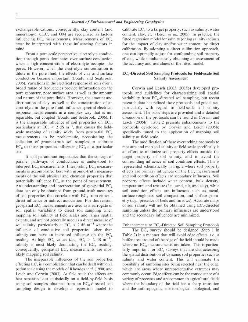
Soil salinity is a dynamic property that is spatially

and temporally complex in nature. Figure 1 visually

indicates the spatially complex salinity patterns that

exist at field scale. The dynamic nature of soil salinity

makes mapping and monitoring of salinity a difficult

challenge. Mapping and monitoring soil salinity at field

scale requires a rapid, reliable, easy means of taking

geospatial measurements. The use of soil samples to

measure salinity at field scales is impractical because

1

JEEG, March 2013, Volume 18, Issue 1, pp. 1–25 DOI: 10.2113/JEEG18.1.1

of the need for hundreds or even thousands of grid

samples. The use of soil samples to measure salinity at

field scales is only practical when sampling is directed to

minimize the number of samples that reflect the range

and variability of salinity within the area of study. This

can be achieved using easily measured spatial informa-

tion that is strongly correlated to soil salinity as a means

of directing where to take the fewest samples. Two

potential sources of correlated spatial information used

to direct where soil samples should be taken to measure

soil salinity as characterized by the electrical conductiv-

ity of the soil saturation extract (ECe) are: 1) visual crop

observations and 2) geospatial measurements of ECa

with mobile electrical resistivity (ER) or electromagnetic

induction (EMI) equipment.

Visual crop observation is a quick method, but it

has a distinct disadvantage, i.e., salinity development is

detected after crop damage has occurred; consequently,

crop yield must be sacrificed to locate areas of salinity

development. Furthermore, visual crop observations

cannot reliably identify low and moderate levels of

salinity. For management purposes, an understanding of

the spatial distribution of low and moderate salinity

levels is just as important as knowing the location of

high salinity. In addition, decreases in crop yield are not

necessarily the consequence of only salt accumulation.

Crops respond to a variety of anthropogenic (e.g.,

irrigation uniformity, farm equipment traffic), edaphic

(e.g., salinity, water content, texture, organic matter),

biological (e.g., disease, nematodes), meteorological

(e.g., precipitation, humidity, temperature), and topo-

graphical (e.g., slope, elevation, microrelief) factors, any

of which can cause yield reduction. Because of the

variety of factors influencing crop yield and quality, the

use of visual crop observations to assess soil salinity is

not definitive and can be extremely misleading.

Associated with visual crop observation, but

considered a distinct potential approach, is the use of

multi- and hyper-spectral imagery. Even though the use

of remote imagery has tremendous potential, at this

point it is still in its infancy and is restricted to research

since protocols have not been developed for general

application to mapping and monitoring salinity. The

research that has been done in the use of remote imagery

to map soil salinity is largely site specific in nature and is

not sufficiently developed to have broad application. At

present, only the use of geospatial measurements of ECa

can provide reliable, accurate maps of salinity at field

scale. Even so, remote imagery will undoubtedly play a

future role in mapping salinity, particularly at regional

scales. The potential of remote imagery in regional-scale

mapping of soil salinity is readily apparent in the recent

work of Lobell et al. (2010).

Since its early agricultural use for measuring soil

salinity, the application of ECa has evolved into a widely

accepted means of establishing the spatial variability

of several soil physical and chemical properties that

influence the ECa measurement, aside from soil salinity

(Corwin and Lesch, 2003, 2005a). Corwin and Lesch

(2005a) provide a compilation of literature pertaining to

the soil physical and chemical properties that are either

directly or indirectly measured by ECa.

Because the geospatial measurement of ECa is a

complex spatially measured property of soil that reflects

the influence of several soil physical and chemical

properties (including soil salinity, clay content and

mineralogy, water content, bulk density, organic matter,

and cation exchange capacity), it is rarely used to map a

single property but rather is used as a surrogate for

general spatial variability of those soil physical and

chemical properties that are spatially correlated with

ECa. As such, geospatial measurements of ECa are used

to direct soil sampling as a means of characterizing

spatial variability of those soil properties that correlate

with ECa at that particularly study site. Characterizing

spatial variability with ECa-directed soil sampling is

based on the notion that when ECa correlates with a soil

property or properties, then spatial ECa information can

be used to identify sites that reflect the range and

variability of the property or properties.

In instances where ECa correlates with a particular

soil property, an ECa-directed soil sampling approach

will establish the spatial distribution of that property

with an optimum number of site locations to character-

ize the variability and keep labor costs minimal (Corwin

et al., 2003a). Details for conducting a field-scale ECa

survey for the purpose of characterizing the spatial

variability of soil properties can be found in Corwin and

Lesch (2005b). General guidelines appear in Corwin and

Lesch (2003) and Corwin et al. (2003a, 2003b).

Figure 1. Aerial view of a typical salt-affected field,showing the complex spatial patterns of salinity.

2

Journal of Environmental and Engineering Geophysics

The mapping of soil salinity at field scale with

ECa-directed soil sampling has a unique set of consid-

erations that was not specifically nor comprehensively

addressed in the prior protocols developed by Corwin

and Lesch (2005b). It is the objective of this review and

analysis paper to provide an overview of the field-scale

characterization of soil salinity distribution using ECa-

directed soil sampling. Protocols, guidelines, special

considerations, and strengths and limitations are dis-

cussed for characterizing spatial and temporal variation

in soil salinity using ECa-directed soil sampling. The

protocols and guidelines are an enhancement and

update of those originally presented by Corwin and

Lesch (2003, 2005b) with a focus on soil salinity.

Original data are presented showing the critical impor-

tance of conducting ECa surveys at or near field

capacity. A case study is presented covering a range of

field-scale salinities to demonstrate the effectiveness of

generating soil salinity maps using ECa-directed soil

sampling. Basic introductory material is presented in the

Appendix to provide background reference information

useful for understanding the relationship between ECa

and soil salinity, which is crucial to the interpretation of

geo-referenced ECa measurements for the purpose of

mapping soil salinity.

Complexity of the ECa Measurement

The interpretation of ECa measurements is not

trivial because of the complexity of current flow in the

bulk soil. Numerous ECa studies have been conducted

that have revealed the site specificity and complexity of

geospatial ECa measurements with respect to the

particular property or properties influencing the ECa

measurement at the study site. Corwin and Lesch

(2005a) provide a compilation of ECa studies and the

associated dominant soil property or properties mea-

sured by ECa for that study. More pertinent to the issue

of soil salinity, Table 1 provides an update of the field

studies that have used ECa to measure and/or map soil

salinity.

The advantages of the ECa measurement are that

it is rapid, reliable, and easy to take, which have made it

an ideal field measurement tool, but because of the

multiple pathways of conductance it is often difficult to

interpret. Corwin and Lesch (2003) provided guidelines

for the use of ECa in agriculture by identifying the

complexities of the ECa measurement and how to deal

with them. Three parallel pathways of current flow

contribute to the ECa measurement: 1) a liquid phase

pathway via salts contained in the soil water occupying

the large pores, 2) a solid pathway via soil particles that

are in direct and continuous contact with one another,

and 3) a solid-liquid pathway primarily via exchange-

able cations associated with clay minerals (Rhoades

et al., 1999b). To measure soil salinity, the electrical

conductance of only the soil solution is required;

consequently, ECa measures more than just soil salinity.

In fact, ECa is a measure of anything conductive within

the volume of measurement and is influenced, whether

directly or indirectly, by any edaphic property that

affects bulk soil conductance.

Because of the pathways of conductance, ECa is

influenced by a complex interaction of edaphic proper-

ties including salinity, saturation percentage (SP), water

content, bulk density (Db), organic matter (OM), cation

exchange capacity (CEC), clay content and mineralogy,

and temperature. The SP and Db are both directly

influenced by clay content and OM (Stiven and Khan,

1966; Rhoades et al., 1990; Gavlak et al., 2003).

Furthermore, the exchange surfaces on clays and OM

provide a solid-liquid phase pathway primarily via

Table 1. Compilation of literature using ECa to measure soil salinity at laboratory, plot, and field scales.

Scale of study References

Laboratory and plot scales site

within a field)

(or singleHalvorson and Rhoades (1976), Rhoades et al. (1976), Rhoades and Corwin

(1981), Corwin and Rhoades (1982, 1984),Wollenhaupt et al. (1986), Rhoades et al.

(1989b, 1990), Corwin and Rhoades (1990), Slavich and Petterson (1990), Hanson and

Kaita (1997), Johnston et al. (1997)

Field scale (or larger spatial extent) de Jong et al. (1979), Cameron et al. (1981), Williams and Baker (1982), Greenhouse and

Slaine (1983), van der Lelij (1983), Williams and Hoey (1987), Rhoades and Corwin (1990),

Diaz and Herrero (1992), Hendrickx et al. (1992), Lesch et al. (1992, 1995a, 1995b, 1998),

Rhoades (1992, 1993), Cannon et al. (1994), Nettleton et al. (1994), Bennett and George

(1995), Mankin et al. (1997), McKenzie et al. (1997), Rhoades et al. (1997, 1999a, 1999b),

Triantafilis et al. (2001), Triantafilis et al. (2002), Mankin and Karthikeyan (2002), Herrero

et al. (2003), Paine (2003), Kaffka et al. (2005), Lesch et al. (2005), Kinal et al. (2006),

Amezketa (2007), Akramkhanov et al. (2008), Urdanoz et al. (2008), Zheng et al. (2009)

3

Corwin and Lesch: Protocols for Field-scale Mapping of Soil Salinity

exchangeable cations; consequently, clay content (and

mineralogy), CEC, and OM are recognized as factors

influencing ECa measurements. Measurements of ECa

must be interpreted with these influencing factors in

mind.

From a pore-scale perspective, electrolyte conduc-

tion through pores dominates over surface conduction

when a high concentration of electrolyte occupies the

pores. However, when the electrolyte concentration is

dilute in the pore fluid, the effects of clay and surface

conduction become important (Boadu and Seabrook,

2006). Variations in the electrical response of soils over a

broad range of frequencies provide information on the

pore geometry, pore surface area as well as the amount

and nature of the pore fluids. However, the amount and

distribution of clay, as well as the concentration of an

electrolyte in the pore fluid, influence spectral electrical

response measurements in a complex way that is not

separable, but coupled (Boadu and Seabrook, 2006). It

is the inseparable influence of soil properties on ECa,

particularly at ECa , 2 dS m21, that causes the field-

scale mapping of salinity solely from geospatial ECa

measurements to be problematic, necessitating the

collection of ground-truth soil samples to calibrate

ECa to those properties influencing ECa at a particular

site.

It is of paramount importance that the concept of

parallel pathways of conductance is understood to

interpret ECa measurements. Interpreting ECa measure-

ments is accomplished best with ground-truth measure-

ments of the soil physical and chemical properties that

potentially influence ECa at the point of measurement.

An understanding and interpretation of geospatial ECa

data can only be obtained from ground-truth measures

of soil properties that correlate with ECa from either a

direct influence or indirect association. For this reason,

geospatial ECa measurements are used as a surrogate of

soil spatial variability to direct soil sampling when

mapping soil salinity at field scales and larger spatial

extents, and are not generally used as a direct measure of

soil salinity, particularly at ECa , 2 dS m21 where the

influence of conductive soil properties other than

salinity can have an increased influence on the ECa

reading. At high ECa values (i.e., ECa . 2 dS m21),

salinity is most likely dominating the ECa reading;

consequently, geospatial ECa measurements are most

likely mapping soil salinity.

The inseparable influences of the soil properties

effecting ECa is a complication that can be dealt with on a

pedon scale using the models of Rhoades et al. (1990) and

Lesch and Corwin (2003). At field scale the effects are

best separated out statistically on a field-by-field basis

using soil samples obtained from an ECa-directed soil

sampling design to develop a regression model to

calibrate ECa to a target property, such as salinity, water

content, clay, etc. (Lesch et al., 2005). In practice, the

fitted regression model for salinity (or log salinity) adjusts

for the impact of clay and/or water content by direct

calibration. By adopting a direct calibration approach,

one can optimally adjust for confounding soil property

effects, while simultaneously obtaining an assessment of

the accuracy and usefulness of the fitted model.

ECa-Directed Soil Sampling Protocols for Field-scale Soil

Salinity Assessment

Corwin and Lesch (2003, 2005b) developed pro-

tocols and guidelines for characterizing soil spatial

variability from ECa-directed soil sampling, but recent

research data has refined these protocols and guidelines,

particularly with regard to field-scale soil salinity

assessment. The basic steps are provided and a detailed

discussion of the protocols can be found in Corwin and

Lesch (2005b). Table 2 presents enhancements to the

protocols developed by Corwin and Lesch (2005b)

specifically tuned to the application of mapping soil

salinity at field scale.

The modification of these overarching protocols to

measure and map soil salinity at field scale specifically is

an effort to minimize soil property effects outside the

target property of soil salinity, and to avoid the

confounding influence of soil condition effects. This is

represented schematically in Fig. 2 where soil property

effects are primary influences on the ECa measurement

and soil condition effects are secondary influences. Soil

property effects include water content, bulk density,

temperature, and texture (i.e., sand, silt, and clay), while

soil condition effects are influences such as metal,

surface roughness, soil compaction, and surface geom-

etry (e.g., presence of beds and furrows). Accurate maps

of soil salinity will not be obtained using ECa-directed

sampling unless the primary influences are understood

and the secondary influences are minimized.

Enhancements to ECa-Directed Soil Sampling Protocols

The ECa survey should be designed (Step 1 in

Table 2) in a manner that will avoid edge effects, i.e., a

buffer area around of the edge of the field should be made

where no ECa measurements are taken. This is particu-

larly important for ECa surveys that are characterizing

the spatial distribution of dynamic soil properties such as

salinity and water content. This will eliminate the

possibility of sampling sites being selected near the edge,

which are areas where unrepresentative extremes may

commonly occur. Edge effects can be the consequence of a

variety of processes and are common to agricultural fields

where the boundary of the field has a sharp transition

and the anthropogenic, meteorological, biological, and

4

Journal of Environmental and Engineering Geophysics

Table 2. Outline of steps to conduct an ECa field survey to map soil salinity. Modified from Corwin and Lesch (2005b)specifically for mapping soil salinity.

1. Site description and ECa survey design

a. record site metadata

b. define the project’s/survey’s objective (e.g., inventorying, spatio-temporal monitoring, site-specific management, etc.)

c. establish site boundaries

d. select GPS coordinate system

e. establish ECa measurement intensity (i.e., number and location of traverses and space between ECa measurements with careful

consideration of edge effects)

f. minimize secondary influences on ECa (e.g., compaction, surface roughness and geometry, metal)

g. special ECa survey design considerations

(1) presence of beds and furrows: perform separate surveys for the beds and for the furrows

(2) vineyards with metal trellising

(a) maximize distance from metal for surveys with EMI

(b) place an insulator between metal posts and trellis wires to break the conductance loop from the soil to the posts along

the wires and back into the soil (this applies to both ER and EMI surveys)

(3) presence of drip lines: perform separate ECa surveys over and between drip lines

(4) variations in surface geometry or roughness: perform separate surveys with separate sampling designs for each area differing

in surface roughness or surface geometry

(5) temporal studies

(a) reference all ECa measurement to 25uC or

(b) conduct ECa surveys at same time of day and same day of year

2. ECa data collection with mobile GPS-based equipment

a. conduct drift runs when using EMI to determine the effect of ambient temperature on EMI instrumentation

b. geo-reference site boundaries and significant physical geographic features with GPS

c. assure that water content at study site is at or near field capacity ($70% field capacity) throughout the field (if water content is

,70%, then do not conduct ECa survey)

d. measure geo-referenced ECa data at the pre-determined spatial intensity and record associated metadata

e. keep speed of mobile GPS-based equipment ,10 km hr21 to reduce GPS positional errors

3. Soil sample design based on geo-referenced ECa data

a. statistically analyze ECa data using an appropriate statistical sampling design (i.e., model- or design-based sampling design) to

establish the soil sample site locations

b. establish site locations, depth of sampling, sample depth increments, and number of cores per site (.100 soil samples are desirable

but the total number of samples is largely determined by the resources available to analyze the soil properties of concern)

4. Soil core sampling at specified sites designated by the sample design

a. obtain measurements of soil temperature through the profile at selected sites

b. at randomly selected locations obtain duplicate soil cores within a 1-m distance of one another to establish local-scale variation

of soil salinity (and other soil properties) for 20% or more of the sample locations

c. recordsoilcoreobservations(e.g.,temperature,color,CaCO3,gleying,organicmatter,mottling,horizonation,texturaldiscontinuities,etc.)

5. Laboratory analysis of soil salinity and other ECa-correlated soil properties relevant to the project objectives

6. Stochastic and/or deterministic calibration of ECa to ECe (and to other soil properties, e.g., water content, SP, etc.)

7. Spatial statistical analysis to determine the soil properties influencing ECa

a. perform a basic statistical analysis of soil salinity (and other relevant soil properties) by depth increment and by composite

depth over the depth of measurement of ECa

b. determine the correlation between ECa and salinity (and between ECa and other soil properties) by composite depth over the

depth of measurement of ECa

8. GIS database development

9. Graphic display of spatial distribution of soil salinity (and other properties correlated to ECa) using various interpolation

methods (e.g., inverse distance weighting, cubic spline, geostatistics)

5

Corwin and Lesch: Protocols for Field-scale Mapping of Soil Salinity

edaphic factors influencing plants (or animals) are not

representative of the field as a whole. As an example,

runoff from roads surrounding a field can cause increased

leaching of salts and higher water contents at the edges of

fields. Salts used to de-ice roads at the edge of fields canaccumulate. Higher temperatures and lower relative

humidity at the edges of a field can cause increased

evapotranspiration, which reduces leaching and lowers

water contents, thereby increasing salinity. These and

other processes can result in salinity and water content

levels at the edges of fields that are not representative and

do not reflect the processes occurring throughout the rest

of the field; consequently, a buffer area around the field isrecommended where no ECa measurements are taken so

that the sampling design is not influenced by unrepresen-

tative edge effects.

The issue of edge effects influencing the sampling

design is of particular concern for the response surface

sampling design used in the ESAP software developed

at the U.S. Salinity Laboratory by Lesch et al. (2000)

because the software identifies sampling sites by mini-mizing clustering, which often results in the identifica-

tion of sites near the edge. To combat the influence of

edge effects, ESAP has a built-in means of creating a

buffer area at the edge of a field where ECa measure-

ments can be omitted.

As a rule-of-thumb for a rectangular field, the first

and last traverses and the start and end of each traverse

using mobile geo-referenced ECa equipment should be adistance of 0.5(w/n) and 0.5(d/n), respectively, from the

edge of the field to avoid edge effects (the distance

between traverses is d/n), where w is the width of the

field, d is the length of the field and n is the number of

desired ECa traverses. For non-rectangular fields, the

first and last traverses and the start and end of each

traverse can be 0.5(w/n) from the edge of the field, where

w is now the greatest width of the field. This rule-of-thumb is of greatest importance when a small number of

soil sample sites are selected (e.g., ,10), whether by a

model- or designed-based sampling strategy, from a

minimal number of traverses (e.g., ,10). Concern for

edge effects becomes less of an issue as the number of

traverses and soil sample sites increases.

An example of an edge effect can be seen in the

ECa survey of a drip-irrigated vineyard in the Caneros

region of California’s Napa Valley (38u 159 53.00 lat., 122u199 48.14 long.). An ECa survey using a Geonics dual-

dipole EM38 was conducted on a 1.8-ha block following

the protocols presented in Table 2. Measurements were

taken approximately 5 m apart and were taken both in the

vine row and between vine rows (Fig. 3(a)). Metal trellises

supporting the vines and drip lines were present in the

vine row. In addition to EMI measurements, ER

measurements of ECa were taken at the same locations

using a Biddle electrical resistivity meter with a Wenner

array configuration and an inter-electrode spacing of

0.75 m for the four stainless-steel electrodes. Measure-

ments of ECa were taken with no consideration for a

buffer zone around the edge of the field since a large

number of traverses (29 traverses) were conducted

(Fig. 3(a)). The EMI measurements of ECa at the edges

Figure 3. Napa Valley (Caneros Region) ECa survey of

a vineyard using electromagnetic induction: a) in-row and

between row sites and b) EMh and EMv measurements

between and in row.

Figure 2. Conceptual path diagram of the primary andsecondary factors influencing an ECa survey targeted at

measuring soil salinity.

6

Journal of Environmental and Engineering Geophysics

of the vineyard block are consistently lower (Fig. 3(b)).

The lower ECa measurements on the edges are a

consequence of anthropogenic (use of a desiccant on the

road surrounding the block to reduce road slickness),

topographic (gentle downhill slope from west to east), and

meteorological (lower relative humidity) influences, which

influence the water content distribution at the edges of the

block. The large number of traverses (i.e., 29 traverses)

clearly identifies these as edge effects. When large

numbers of traverses are taken, edge effects do not

disproportionately influence the sample design, but when

few traverses are taken, the sampling design can be

unduly influenced by less representative extreme ECa

values that are the result of processes confined mainly to

the edge of the field. The average EMh (EMh is the

measurement taken with the EM38 in the horizontal

position) for the 29 in-row traverses is 0.78 dS m21, while

for 5 in-row traverses with the traverses starting and

ending at the edge of the block the average EMh is

0.72 dS m21; for 5 traverses following the 0.5(w/n) rule-of-

thumb the average EMh is 0.80 dS m21. The drier edges of

the vineyard block have a greater influence on lowering

the field average for EMh when a buffer area around the

field is not used.

Another aspect of Step 1 that needs consideration

specific to surveys of vineyards is the influence of metal,

particularly metal trellises. Metal trellises in vineyards

pose a challenge to ECa surveys, both for EMI and for

ER. Use of EMI for surveys of ECa within vineyards with

metal trellising have shown that the metal trellis distorts

the ECa values, causing increases as high as 0.50 dS m21

or more (Lamb et al., 2005). Close attention needs to be

given to take EMI measurements of ECa sufficiently far

from any metal post and trellis wires to eliminate any

magnetic influence on the EMI conductivity reading. The

ECa survey shown in Fig. 3(b) took the metal posts and

wires of the trellises into account by positioning the

EM38 midway between surrounding metal posts and

keeping the EM38 at ground level away from the trellis.

This was done for both in-row and between-row

measurements. When the trellises were ignored and

EMI measurements were taken without regard for the

position of nearby metal posts, the average EMh and

EMv (EMv is the measurement taken with the EM38 in

the vertical position) were roughly 0.10 dS m21 higher,

which are spurious elevated results resulting from the

influence of metal. When trellises in a vineyard are

comprised of steel posts, Lamb et al. (2005) recom-

mended that EMI surveys should only be conducted

where the row spacing is 3 m or more and traverses are

made mid-row.

A relavent question arises, is the increase in the

average EMh and EMv due strictly to the magnetic

influence of the metal trellis? A correlation analysis

between ECa values obtained with an EM38 in the

horizontal coil configuration (EMh) and ER (i.e., four-

electrode Wenner array with a 0.75-m inter-electrode

spacing) for in-row and for between-row ECa surveys of

the Napa Valley vineyard shows high correlations of

R 5 0.92 and 0.97, respectively. Similarly, the spatial

patterns between EMI and ER instruments are virtually

the same. This suggests that there is not only a magnetic

influence but that there is a continuous conductance

loop that extends from the soil up through the metal

post, along the trellis, back down the adjacent metal

post, and returning into the soil. This conductance loop

is measured with both EMI and ER. The lower

correlation for the in-row ER and EMI ECa measure-

ments (i.e., R 5 0.92) than for the between-row

measurements (i.e., R 5 0.97) is presumably caused by

the added magnetic influence on the EMI measure-

ments.

Ostensibly, the influence of metal trellises is not

solely a magnetic effect that only influences EMI and

not ER. The fact that ER is not affected by magnetic

influences caused by the presence of metal does not

cause it to be the instrument of choice for vineyards with

metal trellises. The presence of metal trellises is

problematic for both EMI and ER because the metal

posts and trellis wires potentially serve as a continuous

conductance loop. To remove this influence of metal on

either ER or EMI, the conductance loop must be

broken, which can be accomplished by inserting an

insulator between the metal posts and trellis wires. For

numerous geo-referenced ECa measurements, the inser-

tion of an insulator between all trellis wires and

supporting posts is likely impractical. However, as long

as the trellis system configuration (i.e., spacing of posts,

dripper guide-wire, and cordon, gripper, and foliage

wires) remains the same and measurements are taken in

the same position relative to the trellis, the metal

influences the absolute ECa values similar to ‘‘back-

ground noise.’’

The presence of beds and furrows and drip

irrigation requires special ECa survey considerations

because of the abrupt changes that occur in water content

and salt accumulation. Flood irrigation down furrows

causes the lateral and upward flow of salts into beds. To

get a comprehensive understanding of the salinity

distribution, separate ECa surveys are needed for the

furrow and for the bed. Similarly, abrupt changes in

water content and salinity distribution occur under drip

irrigation. To get a more realistic understanding of soil

salinity distribution in fields under drip irrigation, field-

scale ECa surveys should be conducted so that traverses

are made within and between drip lines. Figure 3(b)

shows the dramatic difference in the spatial patterns and

magnitude of ECa as measured with EMh for in-row and

7

Corwin and Lesch: Protocols for Field-scale Mapping of Soil Salinity

between-row traverses of the drip-irrigated vineyard in

Napa Valley. The in-row average ECa (EMh 5

0.75 dS m21) is higher than between-row average ECa

(EMh 5 0.52 dS m21) because of the higher water content

below the drip lines. The complex three-dimensional

nature of salt and water distribution under drip irrigation

cannot be understood without surveying both within and

between drip lines to avoid misinterpretation of the

spatial ECa information concerning water content and

soil salinity.

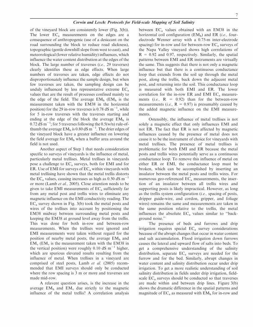
The ECa survey design (Step 1) must also consider

the surface roughness (i.e., smooth or disked surface)

and surface geometry (i.e., presence and absence of beds

and furrow). As an example, Fig. 4 shows an EMI

survey of ECa (i.e., EMh) of a field where the northern

end was disked flat and the southern end was in beds

and furrows. As can be seen, there is a sharp boundary

between the flat disked area and bed-furrow area,

showing the influence of the presence of beds and

furrows, which is a result of salt accumulation in the

beds caused by the lateral and upward flow of leached

salts from the furrow into the bed. The roughness of the

soil surface can also influence spatial ECa measure-

ments. Geospatial measurements taken on a smooth

field surface will be higher than the same field with a

rough surface from disking. This is because of the fact

that the disturbed disked soil acts as an insulating layer

to the conductance pathways, thereby reducing its

conductance. The extent of the reduction in conductance

depends upon the depth of the plow layer and the

coarseness of the clods. When conducting a geospatial

ECa survey of a field, the entire field must have the same

surface roughness and same surface geometry.

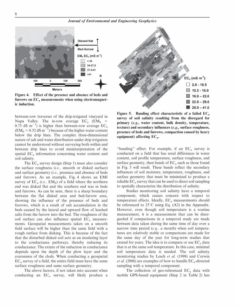
The above factors, if not taken into account when

conducting an ECa survey, will likely produce a

‘‘banding’’ effect. For example, if an ECa survey is

conducted on a field that has areal differences in water

content, soil profile temperature, surface roughness, and

surface geometry, then bands of ECa such as those found

in Fig. 5 will result. These bands reflect the secondary

influences of soil moisture, temperature, roughness, and

surface geometry that must be minimized to produce a

reliable ECa survey that can be used to direct soil sampling

to spatially characterize the distribution of salinity.

Studies monitoring soil salinity have a temporal

component, which causes concern with respect to

temperature effects. Ideally, ECa measurements should

be referenced to 25uC using Eq. (A2) in the Appendix.

However, even though soil temperature is a routine

measurement, it is a measurement that can be disre-

garded if comparisons in a temporal study are made

between data taken during the same time of day over a

narrow time period (e.g., a month) when soil tempera-

tures are relatively stable or comparisons are made for

the same day of the year for long-term studies that

extend for years. The idea is to compare or use ECa data

that is at the same soil temperature. In this case, minimal

soil temperature data is needed. The soil salinity

monitoring studies by Lesch et al. (1998) and Corwin

et al. (2006) are examples of how to handle ECa-directed

sampling with a temporal component.

The collection of geo-referenced ECa data with

mobile GPS-based equipment (Step 2 in Table 2) has

Figure 4. Effect of the presence and absence of beds and

furrows on ECa measurements when using electromagnet-

ic induction.

Figure 5. Banding effect characteristic of a failed ECa

survey of soil salinity resulting from the disregard for

primary (e.g., water content, bulk density, temperature,

texture) and secondary influences (e.g., surface roughness,presence of beds and furrows, compaction caused by heavy

equipment) affecting ECa.

8

Journal of Environmental and Engineering Geophysics

associated concerns that were not identified in the

protocols of Corwin and Lesch (2005b), including drift

runs to determine the effect of ambient temperature on

EMI instrumentation and the range of water contents

over which the ECa data must be collected to assure

reliable data due to contiguous conductance pathways

through the solution phase. A study by Robinson et al.

(2004) indicated that drift commonly observed in the

EM38 is likely caused by temperature effects on the

EM38 sensor and that a simple reflective shade over

the sensor could reduce drift effects considerably.

However, an added precaution would be to conduct

regular ‘‘drift runs’’ where repeated data is periodically

acquired throughout the day along the same transect to

adjust for the drift in the post-processing of ECa data.

Drift runs are generally conducted in the morning,

noon, and late afternoon to provide a range of diurnal

temperature effects on the EM instrument. The varia-

tions in drift provide the basis for adjusting the ECa

measurements. As a rule-of-thumb, normalization of

ECa data using the drift runs should occur when

successive drift runs are shifted by $5%.

The original general protocols by Corwin and

Lesch (2005b) indicated that ECa surveys should be

conducted at or near field capacity, but did not specify

the range of water contents. Original field data is

presented in the following subsection entitled Impor-

tance of Water Content in ECa-Directed Soil Sampling

for Field-Scale Salinity Assessment, which identifies the

range of water contents necessary to maintain contigu-

ous conductance pathways for a reliable ECa survey.

Failure to conduct an ECa survey within the identified

range of water contents can result in spurious data that

will render false conclusions about salinity distributions.

Once a geo-referenced ECa survey is conducted,

the data are used to establish the locations of the soil core

sample sites for calibration of ECa to the electrical

conductivity of the extract from a saturated paste (ECe) of

the soil sample (Step 3). To establish the locations where

soil cores are to be taken, either design-based or model-

based sampling schemes can be used (Corwin and Lesch,

2005b). Design-based sampling schemes (e.g., simple

random sampling, stratified random sampling, unsuper-

vised classification, etc.) have historically been the most

commonly used and hence are more familiar to most

research scientists. The validity and effectiveness of a

sampling strategy is fundamental to the ECa-directed soil

sampling approach. Recent validation and comparison

studies of model- and design-based sampling strategies for

characterizing the spatial variability of soil salinity with

ECa-directed soil sampling have indicated that the model-

based sampling approach resulted in better model

discrimination, more precise parameter estimates, and

smaller prediction variances than the design-based

sampling strategy (Lesch and Corwin, 2008; Corwin

et al., 2010). Even though a model-based sampling design,

such as a response surface sampling design, has been less

prevalent in the literature, it is concluded from the

comparison that there is no reason to refrain from its use

and, in fact, warrants equal consideration. The clear

advantage of the model-based sampling design, and more

specifically the use of a response surface sampling design,

is that there is a substantial reduction in the number

of samples required to characterize the variation in soil

salinity as compared to other approaches. A drawback is

that the level of technical knowledge in the use of software

such as ESAP (Lesch et al., 2000), which uses the response

surface sampling design approach, is greater than other

statistical software.

A crucial aspect of Step 4 in Table 2, which has

been largely overlooked in many past ECa-directed soil

sampling studies listed in Table 1 and deserving of

attention, is that of establishing the local-scale variation

through duplicate or replicate samples at 20% or more

of the sample sites. Knowledge of the local-scale

variation in comparison to global-scale variation is

important since this helps to define sampling require-

ments (i.e., number of replicates) and provide a per-

spective to the small- and large-scale variation in salinity

that occurs within a field. If the local-scale variation in

salinity approaches global-scale variation, then there is

just as much variation within a small area (e.g., 1 m2) as

over the entire field, which makes the ECa-directed

sampling approach untenable.

Steps 5–8 in Table 2 are the same as the original

protocols by Corwin and Lesch (2005b).

Step 9 in Table 2 focuses on the methods of

interpolation that are available to display the spatial

distribution of soil salinity. Inverse distance weighting,

cubic spline, and various geostatistical approaches are

the prevalent choices. Previous studies comparing

interpolation methods have met with mixed results;

consequently, jackknifing is often used to establish the

interpolation method that minimizes prediction error

(Isaaks and Srivastava, 1989). Bourgault et al. (1997)

provide a useful toolbox of geostatistical approaches

used on a soil salinity data set and advise the use of

cross-validation to decide the approach that is best.

The advantage of using a geostatistical approach for

interpolation over inverse distance weighting or cubic

spline is an assessment of spatial uncertainty that can be

obtained from geostatistical approaches.

Importance of Water Content in ECa-Directed Soil

Sampling for Field-scale Salinity Assessment

The ECa survey protocols of Corwin and Lesch

(2005b) emphasized the importance of conducting ECa

surveys in fields where the water content was at or near

9

Corwin and Lesch: Protocols for Field-scale Mapping of Soil Salinity

field capacity across the entire field. Field capacity refers

to the water content at approximately 1/3 bar and in the

field is taken to represent the water content at which free

drainage no longer occurs, which generally occurs 2–

4 days following a rainfall or irrigation (Peters, 1965).

Presented herein is empirical data from two field studies

illustrating over what range of water contents field-scale

ECa surveys must be conducted to provide reliable

results.

Site locations of ECa surveys. Surveys of ECa were

conducted at two field sites, one near Roswell, New

Mexico (33u 239 140 N, 104u 319 410 W) and the other

outside Sterling, Colorado (40u 359 02.7950 N, 103u 009

34.8440 W). The Roswell, NM site is a center-pivot

irrigated field of approximately 95 ha. The circular field

was subdivided into two fields, one in the north of 41 ha

and one in the south of 54 ha. The Sterling, CO site

consisted of four contiguous fields. The combined area

of the four contiguous fields was 130 ha. The soil is

predominantly Platner loam (fine, smectitic, mesic

Aridic Paleustolls), Weld loam (fine, smectitic, mesic

Aridic Argiustolls), and Rago loam (fine, smectitic,

mesic Pachic Argiustolls).

ECa surveys. The ECa surveys for the Roswell,

NM and Sterling, CO field sites were conducted using

mobile EMI equipment following the protocols outlined

by Corwin and Lesch (2005b), with the exception that

close attention was not given to the water content of the

soil at the time of the surveys, resulting in areas at both

sites that were considerably less than field capacity.

Surveys of ECa were confined to 7-ha sub-sections

in the northern and southern sections of the Roswell,

NM site. In each sub-section, seven (7) east-west

traverses were made with geo-referenced ECa measure-

ments taken with the EM38 in the horizontal (EMh) and

vertical (EMv) positions every 5 m. From the two ECa

surveys, six (6) sampling sites were selected in each sub-

section (north and south) using ESAP software (Lesch

et al., 2000). Soil samples were taken at 0.3-m in-

crements to a depth of 1.2 m. The soil samples were

analyzed for salinity (ECe, dS m21), gravimetric water

content (hg, g g21), and saturation percentage (SP)

following the methodologies provided by Rhoades

(1996). Field capacity was estimated for each depth

increment from field samples taken at each of the 6

sampling sites 2–3 days after irrigation according to the in

situ field capacity method of Cassel and Nielson (1986).

The four contiguous fields in Sterling, CO were

surveyed in April 2005 using mobile EMI equipment

with traverses every 15 m and measurements of EMh

and EMv taken with the EM38 every 5 m along each

traverse. In addition, an ECa survey using mobile ER

equipment (i.e., Veris 3,1001) was conducted so that

each traverse with the Veris 3,100 went over the same

traverse as the mobile EMI equipment. Measurements

of ECa were obtained with the Veris 3,100 at depths of

0–0.3 m and 0–0.9 m. Ten samples sites were selected in

each field using a response surface sampling design

(RSSD), and 9 sites were selected in each field using an

unsupervised classification sampling design (UCSD) for

a total of 76 sites over the four fields. Soil samples were

obtained at depth increments of 0–0.15, 0.15–0.3, 0.3–

0.6, 0.6–0.9, and 0.9–1.2 m. The soil samples were

analyzed for ECe (dS m21), bulk density (rb, g cm23), hg

(g g21), SP, and clay content (g kg21). The analytical

procedure outlined by Rhoades (1996) was used for ECe,

hg, and SP. Clay content and rb were obtained using the

hydrometer method of Gee and Or (2002) and the core

method of Grossman and Reinsch (2002), respectively.

The field capacity for each of the five depth increments

for each field was determined using the ceramic pressure

plate method at 1/3 bar for disturbed soil samples.

Results and discussion. Table 3 presents ECa-

directed sampling data for the north and south sub-

sections of the center-pivot irrigated field in Roswell,

NM. The average ECa measurements in the north are

significantly higher than in the south for both EMh and

EMv (Table 3a). The average ECas in the north are

above 1 dS m21 (i.e., 1.55 and 1.70 dS m21 for EMh and

EMv, respectively), which suggests that salinity is the

soil property most likely responsible for the high ECas.

The low average ECas in the south suggest that the

south has a low salinity level. However, Table 3b shows

that both north and south sub-sections have similar

salinity levels at all depths; both north and south sub-

sections are high in salinity (i.e., 12–15 ds m21). The SP,

which is reflective of the soil texture in low OM soils of

the arid southwestern USA, does not explain the

difference in average ECas between north and south

since both sub-sections have similar SPs at all depths.

The discrepancy in average ECa between north and

south is caused by water content. When water content is

expressed as the percent of field capacity, there is a

distinct difference between the north and south sub-

sections, where the north is wetter than the south. The

data suggest that between 50–70% of field capacity the

conductance pathways in the solution phase are broken,

causing spurious ECa measurements. The importance of

being at or near field capacity when conducting an ECa

survey is substantiated by a comparison of the

correlation of ECa (for EMv) to ECe (for the composite

1 Veris Technologies, Salina, KS, USA. Product identifica-tion is provided solely for the benefit of the reader and doesnot imply the endorsement of the USDA.

10

Journal of Environmental and Engineering Geophysics

depth of 0–1.2 m) between the north and south sub-

sections. The correlation coefficient is 0.93 for the north

and 0.36 for the south, where the percent of field

capacity is 80.3% for the north and 42.0% for the south

for the 0–1.2 m composite depth. Consequently, the ECa

measurements (both EMh and EMv) are not reliable for

the south sub-section because the water content is ,50%

of field capacity, which disrupts the liquid phase con-

ductance pathway.

Table 4 presents corroborating data indicating

that $70% of field capacity is needed down to the

depth of penetration of the geophysical approach (e.g.,

ER or EMI) used to measure ECa to prevent spurious

results from occurring caused by discontinuous conduc-

tance pathways in the soil solution phase. No correla-

tion was found between ECa as measured with EMI and

any of the soil properties expected to influence ECa at

any composite depth. This was true for both EMh,

which measures down to a depth of roughly 0.75 m, and

EMv, which measures to a depth of about 1.5 m.

Ostensibly, the lack of correlation is because of the fact

that the water content was too low over the depths of

penetration of the EMI measurements. The water

content was 49% of field capacity for 0–0.6 m, 42% of

field capacity for 0–0.9 m, and 39% of field capacity for

0–1.2 m. However, the measurement of ECa with ER did

correlate with salinity (ECe) and hg over the 0–0.3 m

increment, which was because of the fact that the water

content was greater than 70% of field capacity

(specifically measured to be 77% of field capacity) in

the top 0.3 m of soil. The water content for 0–0.6 m

dropped to 49% of field capacity and concomitantly the

correlation coefficient between ECa and ECe dropped to

0.11 and between ECa and hg dropped to 0.31. These

results are compatible with the need for water contents

$70% of field capacity for the conductance pathways in

the solution phase to be open.

As a rule-of-thumb, geo-referenced ECa data

collection (Step 2) should be conducted only when the

water content through the soil profile of interest is$70% of field capacity and preferably as close to field

capacity as possible. A gray area exists in the range of

50–70% of field capacity. Surveys of ECa are substan-

tially affected at #50% of field capacity and should not

be conducted on soils that are this dry. Sufficient water

content is needed down to the depth of penetration of

the geophysical approach that is used to prevent

spurious and misleading measurements that wouldsuggest that no salinity was present when actually there

was. This has significant ramifications, particularly for

ECa surveys conducted on dryland farms, since ECa

surveys should only be conducted after sufficient rainfall

has occurred (or sufficient irrigation water has been

applied on irrigated crop land) to wet up the soil profile

to the appropriate depth of penetration of the ECa

measurement instrumentation. If this precaution is nottaken, the reliability of the ECa survey is dubious.

Case Study of Field-scale Soil Salinity Assessment

Study Site Description

The on-farm research study site (lat. 33u 509 25.430

N, long. 117u 009 14.930 W) is located on Scott Brothers’

Dairy Farm in San Jacinto in southern California’s

Table 3. Apparent soil electrical conductivity (ECa) directed sampling data for the north and south sub-sections of a 95-ha center-pivot irrigated field in Roswell, NM: a) average ECa for the electromagnetic induction (EMI) measurements in

the horizontal (EMh) and vertical (EMv) coil configurations and b) associated averages of the soil properties of salinity

(ECe), saturation percentage (SP), and water content (expressed as percent of field capacity) by depth increment for 6

sample sites in each sub-section.

North South

(a) Average ECa (dS m21)

EMh 1.55 0.06

EMv 1.70 0.41

Depth increment (m)

ECe (dS m21) SP % of field capacity

North South North South North South

(b) Associated averages of soil properties

0–0.3 13.1 13.8 47.5 48.2 75.4 40.2

0.3–0.6 13.3 14.8 43.1 42.8 84.6 40.3

0.6–0.9 14.5 14.8 43.5 39.9 82.0 44.4

0.9–1.2 12.6 13.9 41.5 41.1 79.1 43.2

11

Corwin and Lesch: Protocols for Field-scale Mapping of Soil Salinity

Riverside County. The 32-ha center-pivot irrigated field

site provided an extensive range of spatial variability in

ECa needed to make a real-world evaluation of the

salinity mapping capability outlined in ECa-directed

sampling protocols of Table 2. The field has received

dairy lagoon water since 6 March 2008. The average

ECe, pH, NH4+, NO3

2, PO423 and sodium adsorption

ratio of the dairy lagoon water from March 2008 to June

2009 were 1.63 dS m21, 7.8, 0.94 meq L21, 0.78 meq L21,

0.23 meq L21, and 4.3, respectively.

Intensive EMI Survey

Geospatial ECa measurements were obtained with

the Geonics EM38 dual-dipole electrical conductivity

meter. The ECa survey followed the detailed survey

protocols outlined in Table 2. The ECa survey was

conducted 2–4 June 2009. The survey consisted of

geospatial ECa measurements taken with mobile EMI

equipment where measurements were simultaneously

taken both in the horizontal (EMh) and vertical coil

configurations (EMv), with traverses roughly 7.5-m

apart and measurement sites within each traverse

roughly 5-m apart. Measurements were taken at 7,168

locations on transects running in a north-south direc-

tion. Figure 6 shows the interpolated EMI survey results

for EMh and EM measurements. Table 5a indicates the

ECa summary statistics for all 7,168 sites.

Sampling and Laboratory Analysis

Apparent soil electrical conductivity serves as a

surrogate to characterize the spatial variation of those

soil properties that are found to influence ECa within a

field. Based on the variation in ECa, soil sample sites

were selected that reflect the range and variation in

ECa using a model-based sampling strategy, specifically

the response surface sample design (RSSD) used in

the ESAP software (Lesch et al., 2000). The RSSD

specified 40 locations where soil samples were collected

to map soil salinity, which are shown in Fig. 6. Soil

samples were collected for the following depth incre-

ments: 0–0.15, 0.15–0.30, 0.30–0.60, 0.60–0.90, 0.90–

1.20, 1.20–1.50, 1.50–1.80 m. Saturation extracts of the

soil sample depth increments were prepared and the

electrical conductivity of the saturation extracts (ECe,

Table 4. Correlation coefficients between ECa (from electrical resistivity (ER) and electromagnetic induction (EMI)) andsoil properties (salinity (ECe), bulk density (rb), gravimetric water content (hg), and saturation percentage (SP)) at

composite depths for Sterling, CO. EMv represents the EMI measurement in the vertical coil configuration and EMh

represents the EMI measurement in the horizontal coil configuration: a) response surface sampling design (RSSD) sites, b)

unsupervised classification sampling design (UCSD) sites, and c) RSSD and UCSD sites.

Depth increments (cm)

ER EMv EMh Number of samples

Soil property 0–30 0–90 0–15 0–30 0–60 0–90 0–120 0–15 0–30 0–60 0–90 0–120 0–15 0–30 0–60 0–90 0–120

(a) RSSD sites

ECe 0.58 20.05 20.25 20.21 20.19 20.18 20.08 20.21 20.26 20.23 20.17 20.11 40 40 40 36 26

rb 0.43 0.16 20.27 20.18 20.01 20.21 0.004 20.21 0.10 0.41 0.18 0.27 40 40 40 38 31

hg 0.64 0.02 0.27 0.23 0.21 0.32 0.07 0.55 0.60 0.34 0.46 0.46 40 40 40 38 31

SP 0.30 20.38 20.09 20.05 20.14 20.37 20.22 20.41 20.22 20.17 20.40 20.40 40 40 40 36 26

Clay 0.29 20.28 20.06 0.09 20.26 20.42 20.22 20.05 0.11 20.29 20.47 20.22 40 40 40 38 31

(b) UCSD sites

ECe 0.85 0.33 20.42 20.49 20.07 0.02 0.27 20.17 20.11 0.32 0.46 0.75 36 36 36 25 15

rb 0.47 0.35 0.16 0.06 20.01 20.23 20.14 0.49 0.41 0.20 0.08 0.04 36 36 36 31 20

hg 0.83 0.21 20.45 20.37 20.24 20.16 20.15 20.56 20.42 20.39 20.40 20.261 36 36 36 30 19

SP 0.47 20.19 20.44 20.20 20.17 20.14 20.06 20.39 20.02 20.03 20.08 20.12 36 36 36 25 15

Clay 0.33 20.22 20.01 0.44 20.15 20.32 20.25 0.07 0.27 20.40 20.1 20.37 36 36 36 31 19

(c) RSSD and UCSD sites

ECe 0.71 0.13 20.21 20.26 20.14 20.11 20.07 20.14 20.21 0.01 0.05 0.24 76 76 76 61 41

rb 0.45 0.25 0.09 0.13 0.08 0.07 20.02 0.18 0.47 0.24 0.28 0.30 76 76 76 69 51

hg 0.73 0.11 20.16 20.27 20.13 20.17 20.14 20.01 20.17 0.01 20.05 0.00 76 76 76 68 49

SP 0.38 20.29 20.26 20.10 20.14 20.26 20.16 20.18 20.13 20.11 20.26 20.32 76 76 76 61 41

Clay 0.31 20.25 20.25 0.20 20.21 20.36 20.18 20.26 0.15 20.32 20.49 20.24 76 76 76 69 50

12

Journal of Environmental and Engineering Geophysics

dS m21) were measured using the method presented in

Rhoades (1996), which also provides instructions for

measuring hg and SP. Bulk density (rb) was obtained

using the core method of Grossman and Reinsch

(2002). Table 5b provides the summary statistics for

ECe, rb, hg, and SP.

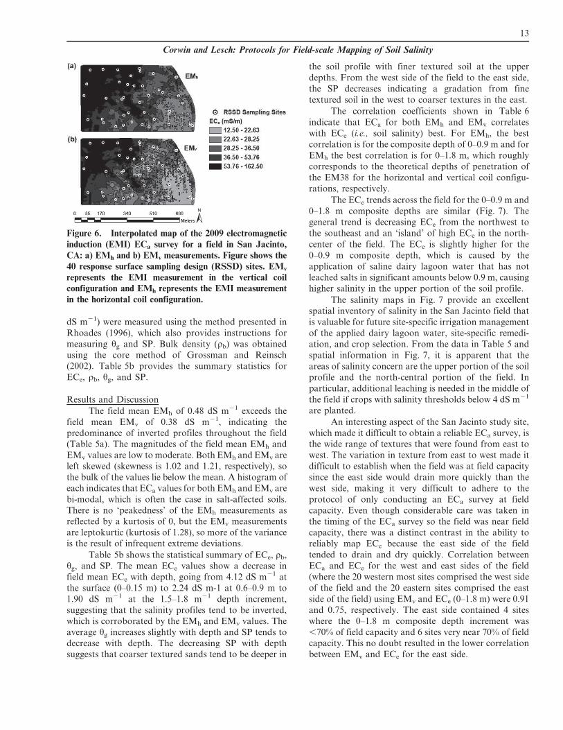
Results and Discussion

The field mean EMh of 0.48 dS m21 exceeds the

field mean EMv of 0.38 dS m21, indicating the

predominance of inverted profiles throughout the field

(Table 5a). The magnitudes of the field mean EMh and

EMv values are low to moderate. Both EMh and EMv are

left skewed (skewness is 1.02 and 1.21, respectively), so

the bulk of the values lie below the mean. A histogram of

each indicates that ECa values for both EMh and EMv are

bi-modal, which is often the case in salt-affected soils.

There is no ‘peakedness’ of the EMh measurements as

reflected by a kurtosis of 0, but the EMv measurements

are leptokurtic (kurtosis of 1.28), so more of the variance

is the result of infrequent extreme deviations.

Table 5b shows the statistical summary of ECe, rb,

hg, and SP. The mean ECe values show a decrease in

field mean ECe with depth, going from 4.12 dS m21 at

the surface (0–0.15 m) to 2.24 dS m-1 at 0.6–0.9 m to

1.90 dS m21 at the 1.5–1.8 m21 depth increment,

suggesting that the salinity profiles tend to be inverted,

which is corroborated by the EMh and EMv values. The

average hg increases slightly with depth and SP tends to

decrease with depth. The decreasing SP with depth

suggests that coarser textured sands tend to be deeper in

the soil profile with finer textured soil at the upper

depths. From the west side of the field to the east side,

the SP decreases indicating a gradation from fine

textured soil in the west to coarser textures in the east.

The correlation coefficients shown in Table 6

indicate that ECa for both EMh and EMv correlates

with ECe (i.e., soil salinity) best. For EMh, the best

correlation is for the composite depth of 0–0.9 m and for

EMh the best correlation is for 0–1.8 m, which roughly

corresponds to the theoretical depths of penetration of

the EM38 for the horizontal and vertical coil configu-

rations, respectively.

The ECe trends across the field for the 0–0.9 m and

0–1.8 m composite depths are similar (Fig. 7). The

general trend is decreasing ECe from the northwest to

the southeast and an ‘island’ of high ECe in the north-

center of the field. The ECe is slightly higher for the

0–0.9 m composite depth, which is caused by the

application of saline dairy lagoon water that has not

leached salts in significant amounts below 0.9 m, causing

higher salinity in the upper portion of the soil profile.

The salinity maps in Fig. 7 provide an excellent

spatial inventory of salinity in the San Jacinto field that

is valuable for future site-specific irrigation management

of the applied dairy lagoon water, site-specific remedi-

ation, and crop selection. From the data in Table 5 and

spatial information in Fig. 7, it is apparent that the

areas of salinity concern are the upper portion of the soil

profile and the north-central portion of the field. In

particular, additional leaching is needed in the middle of

the field if crops with salinity thresholds below 4 dS m21

are planted.

An interesting aspect of the San Jacinto study site,

which made it difficult to obtain a reliable ECa survey, is

the wide range of textures that were found from east to

west. The variation in texture from east to west made it

difficult to establish when the field was at field capacity

since the east side would drain more quickly than the

west side, making it very difficult to adhere to the

protocol of only conducting an ECa survey at field

capacity. Even though considerable care was taken in

the timing of the ECa survey so the field was near field

capacity, there was a distinct contrast in the ability to

reliably map ECe because the east side of the field

tended to drain and dry quickly. Correlation between

ECa and ECe for the west and east sides of the field

(where the 20 western most sites comprised the west side

of the field and the 20 eastern sites comprised the east

side of the field) using EMv and ECe (0–1.8 m) were 0.91

and 0.75, respectively. The east side contained 4 sites

where the 0–1.8 m composite depth increment was

,70% of field capacity and 6 sites very near 70% of field

capacity. This no doubt resulted in the lower correlation

between EMv and ECe for the east side.

Figure 6. Interpolated map of the 2009 electromagnetic

induction (EMI) ECa survey for a field in San Jacinto,

CA: a) EMh and b) EMv measurements. Figure shows the

40 response surface sampling design (RSSD) sites. EMv

represents the EMI measurement in the vertical coilconfiguration and EMh represents the EMI measurement

in the horizontal coil configuration.

13

Corwin and Lesch: Protocols for Field-scale Mapping of Soil Salinity

Conclusion

Enhancements to the protocols of Corwin and

Lesch (2005b) have been made that refine the method-

ology for mapping soil salinity at field scale. These

enhancements focused on minimizing primary (e.g.,

water content, temperature, texture) and secondary

influences (e.g., surface geometry and roughness, metal)

that will affect the target soil property of soil salinity. Of

greatest concern is conducting an ECa survey at $70%

of field capacity to assure that contiguous conductance

pathways are present for either ER or EMI. Failure to

do so will result in the breaking off of the solution phase

conductance pathways, which are crucial to the mea-

surement of soil salinity.

These protocol enhancements produce a more

robust set of guidelines to assure reliable field-scale

maps of soil salinity with the implication that future

research on field-scale mapping of soil salinity with ECa-

directed sampling will be based on a standardized

procedure suitable for a spectrum of applications related

to salinity and broad range of conditions (e.g., drip

irrigation, vineyards with trellising, presence of beds and

furrows, temporal studies).

Table 5. San Jacinto, CA: a) 2009 ECa survey data summary statistics and b) associated soil property summary statisticswhere salinity is represented by ECe (dS m21), bulk density is represented by rb (g cm23), gravimetric water content is

represented by hg (g g21), and saturation percentage is represented by SP. EMv represents the EMI measurement in the

vertical coil configuration and EMh represents the EMI measurement in the horizontal coil configuration.

(a) ECa survey summary statistics (N = 7,168 sites)

Statistical parameter EMv (dS m21) EMh (dS m21)

Mean 0.38 0.48

Standard deviation 0.19 0.24

Skewness 1.21 1.02

Kurtosis 1.28 0.00

(b) Soil property summary statistics (N = 40 sites)

Depth increments (cm)

0–15 15–30 30–60 60–90 90–120 120–150 150–180 0–15 15–30 30–60 60–90 90–120 120–150 150–180

Mean Standard deviation

ECe 4.12 3.71 3.13 2.24 2.11 2.65 1.90 1.24 1.74 2.25 1.74 1.69 3.50 1.53

rb 1.36 1.72 1.43 1.31 1.39 1.44 1.43 0.25 0.26 0.22 0.27 0.23 0.34 0.25

hg 0.22 0.21 0.16 0.16 0.24 0.24 0.24 0.04 0.05 0.07 0.08 0.10 0.11 0.11

SP 41.16 39.67 37.08 34.65 34.46 33.39 31.67 3.78 5.40 6.40 8.36 8.27 7.98 7.19

Minimum Maximum

ECe 1.99 1.14 0.76 0.42 0.22 0.23 0.22 6.77 9.39 13.03 7.58 6.87 20.50 5.83

rb 0.70 1.01 0.71 0.77 0.95 0.79 0.81 2.08 2.56 1.79 1.87 1.85 2.15 2.17

hg 0.07 0.07 0.07 0.07 0.06 0.07 0.06 0.27 0.22 0.25 0.35 0.37 0.37 0.41

SP 34.66 30.23 24.89 19.36 22.09 20.90 20.84 50.96 58.27 53.83 53.70 57.53 56.15 49.73

Skewness Kurtosis

ECe 0.35 0.88 2.40 1.49 1.09 3.79 0.93 20.53 1.62 8.90 2.01 0.28 18.01 20.01

rb 0.56 0.47 21.38 20.19 20.05 0.25 0.37 2.39 2.73 2.96 20.63 20.83 20.46 1.75

hg 0.05 0.18 0.71 1.14 0.59 0.17 0.40 20.13 21.17 20.71 0.40 20.68 21.15 20.83

SP 0.35 1.06 0.40 0.66 0.80 0.85 0.68 0.12 2.23 0.25 0.08 0.54 0.72 20.43

Coefficient of variation

ECe 30.03 47.03 72.08 77.51 79.91 131.94 80.51

rb 18.68 15.05 15.57 20.83 16.94 23.32 17.13

hg 26.22 42.86 59.64 70.87 58.32 64.87 61.28

SP 9.19 13.61 17.27 24.12 24.00 23.90 22.70

14

Journal of Environmental and Engineering Geophysics

Even though ECa-directed sampling is widely used

for mapping field-scale salinity, there are definite

advantages, disadvantages, and limitations that deter-

mine where and under what conditions it is best used

and where there might be concerns for its use. There

are three advantages of ECa-directed sampling. First,

it substantially reduces the number of soil samples

compared to grid sampling since it uses geospatial ECa

measurements as a surrogate to establish the optimum

number and location of sample sites to characterize

the range and variability of soil salinity. The reduction

in the number of samples greatly reduces labor and

cost. Second, ECa-directed sampling renders quick and

reliable results that are statistically tied to ground-

truth measurements of ECe from soil samples, so there

is a direct relationship with salinity. Third, EMI is a

non-destructive measurement and ER results in minimal

soil disturbance.

The disadvantages of ECa-directed soil sampling

do not overshadow the advantages, but are nonetheless

worthy of careful consideration by laymen and un-

trained users. First, the complex interactions of various

soil properties and their resulting influences on the ECa

measurement make it a complex measurement that is

often difficult to interpret. Second, ECa-directed sam-

pling requires expensive and technologically sophisti-

cated geophysical and GPS equipment and requires

trained personnel to operate it.

There are three major limitations that determine

the conditions under which ECa-directed sampling must

be used. First, there must be sufficient water content

(i.e., $70% of field capacity) so that continuous

conductance pathways are maintained down to the

depth of penetration of the geophysical approach used

to measure ECa (i.e., ER or EMI). This may be of

particular concern for soils with impermeable layers,

dryland soils, or shallow soils above bedrock. Second,

the ER approach requires good physical contact

between the electrodes and soil surface and, as such,

ER is not generally used in stoney soils or soils with dry

surfaces. Third, fields with wide ranging soil textures

present a challenge since it may become difficult for the

entire field to be at or near field capacity.

Table 6. Correlation coefficients between ECa (from electromagnetic induction (EMI)) and soil properties (salinity(ECe), bulk density (rb), gravimetric water content (hg), and saturation percentage (SP)) at composite depths for San

Jacinto, CA. a) EMv represents the EMI measurement in the vertical coil configuration and b) EMh represents the EMI

measurement in the horizontal coil configuration.

Composite depth (cm)

Property 0–15 0–30 0–60 0–90 0–120 0–150 0–180

(a) EMh

ECe 0.4502 0.5586 0.7198 0.8843 0.8700 0.7747 0.7874

rb 20.1182 20.1092 20.4734 20.5251 20.5290 20.5950 20.5373

hg 0.1253 0.1999 0.4350 0.4882 0.6998 0.6374 0.6511

SP 20.0211 0.0000 0.2398 0.4427 0.5054 0.5113 0.5028

(b) EMv

ECe 0.4412 0.5096 0.6452 0.7035 0.8012 0.8174 0.8327

rb 20.1610 20.0960 20.5098 20.5753 20.5922 20.6653 20.6196

hg 0.1035 0.1916 0.4012 0.4628 0.6042 0.6517 0.6785

SP 0.0031 0.0107 0.2747 0.4809 0.5662 0.5789 0.5675

Figure 7. Interpolated map of soil salinity (ECe, dS

m21) for the field in San Jacinto, CA from the 40 ECa-

directed sampling sites for composite depths of a) 0–0.9 m

and b) 0–1.8 m.

15

Corwin and Lesch: Protocols for Field-scale Mapping of Soil Salinity

Acknowledgments

The authors wish to acknowledge the numerous hours of

diligent technical work that were performed in the field and in

the laboratory by several technicians whose efforts and

conscientiousness were crucial to obtaining the data presented

in this review and analysis, including Kevin Yemoto, Clay

Wilkinson, and Harry Forster. Special acknowledgment and

thanks go to Cliff Landers for his collection of the Roswell, NM

ECa data. The authors thank the technical support and

assistance of Drs. Cinthia Johnson, Eran Segal, Scott Bradford,

and Todd Skaggs on collaborative work. The authors also thank

the hard work of Danielle Rodriguez at the San Jacinto field site.

References

Akramkhanov, A., Sommer, R., Martius, C., Hendrickx,

J.M.H., and Vlek, P.L.G., 2008, Comparison and

sensitivity of measurement techniques for spatial distri-

bution of soil salinity: Irrig. Drainage Syst., 22, 115–126.

Amezketa, E., 2007, Soil salinity assessment using directed soil

sampling from a geophysical survey with electromag-

netic technology: A case study: Spanish J. Agric. Res.,

5(1) 91–101.

Amoozegar-Fard, A., Nielsen, D.R., and Warrick, A.W.,

1982, Soil solute concentration distributions for spatially

varying pore water velocities and apparent diffusion

coefficients: Soil Sci. Soc. Am. J., 46, 3–9.

Barnes, H.E., 1952, Soil investigation employing a new method

of layer-value determination for earth resistivity inter-

pretation: Highway Res. Board Bull., 65, 26–36.

Bennett, D.L., and George, R.J., 1995, Using the EM38 to

measure the effect of soil salinity on Eucalyptus globulus

in south-western Australia: Agric. Water Manage., 27,

69–86.

Biggar, J.W., and Nielsen, D.R., 1976, Spatial variability of

the leaching characteristics of a field soil: Water Resour.

Res., 12, 78–84.

Boadu, F.K., and Seabrook, B., 2006, Effect of clay and

salinity on the spectral electrical response of soils: J.

Environ. Eng. Geophysics, 11, 161–170.

Borchers, B., Uram, T., and Hendrickx, J.M.H., 1997,

Tikhonov regularization of electrical conductivity depth

profiles in field soils: Soil Sci. Soc. Am. J., 61,

1004–1009.

Bourgault, G., Journel, A.G., Rhoades, J.D., Corwin, D.L.,

and Lesch, S.M., 1997, Geostatistical analysis of a soil

salinity data set, in Advances in agronomy, Sparks, D.L.

(ed.), Academic Press, San Diego, California.

Bresler, E., McNeal, B.L., and Carter, D.L., 1982. Saline and sodic

soils, Springer-Verlag, New York, New York, 174–181.

Burger, H.R., 1992. Exploration geophysics of the shallow

subsurface, Prentice Hall PTR, Upper Saddle River,

New jersey.

Cameron, D.R., de Jong, E., Read, D.W.L., and Oosterveld,

M., 1981, Mapping salinity using resistivity and

electromagnetic inductive techniques: Can. J. Soil Sci.,

61, 67–78.

Cannon, M.E., McKenzie, R.C., and Lachapelle, G., 1994,

Soil-salinity mapping with electromagnetic induction

and satellite-based navigation methods: Can. J. Soil Sci.,

74(3) 335–343.

Cassel, D.K., and Nielsen, D.R., 1986, Field capacity and

available water, in Methods of soil analysis, Part 1 –

Physical and mineralogical methods, 2nd ed., Agronomy

Monograph No. 9, Klute, A. (ed.), SSSA, Madison,

Wisconsin, 901–926.

Corwin, D.L., 2002, Solute content and concentration -

Measurement of solute concentration using soil water

extraction: Porous matrix sensors, in Methods of soil

analysis, Part 4-Physcial methods, SSSA Book Series

No. 5, Dane, J.H., and Topp, G.C. (eds.), SSSA,

Madison, Wisconsin, 1269–1273.

Corwin, D.L., 2005, Geospatial measurements of apparent soil

electrical conductivity for characterizing spatial variability,

in Soil-water-solute process characterization: An integrat-

ed approach, Alvarez-Benedi, J., and Munoz-Carpena, R.

(eds.), CRC Press, Boca Raton, Florida, 639–672.

Corwin, D.L., and Hendrickx, J.M.H., 2002, Solute content

and concentration – Indirect measurement of solute

concentration: Electrical resistivity – Wenner array, in

Methods of soil analysis, Part 4-Physcial methods,

Agronomy Monograph No. 9, Dane, J.H., and Topp,

G.C. (eds.), SSSA, Madison, Wisconsin, 1282–1287.

Corwin, D.L., and Lesch, S.M., 2003, Application of soil

electrical conductivity to precision agriculture: Theory,

principles, and guidelines: Agron. J., 95, 455–471.

Corwin, D.L., and Lesch, S.M., 2005a, Apparent soil electrical

conductivity measurements in agriculture: Comput.

Electron. Agric., 46(1–3) 11–43.

Corwin, D.L., and Lesch, S.M., 2005b, Characterizing soil

spatial variability with apparent soil electrical conduc-

tivity: I. Survey protocols: Comput. Electron. Agric.,

46(1–3) 103–133.

Corwin, D.L., and Rhoades, J.D., 1982, An improved

technique for determining soil electrical conductivity-

depth relations from above-ground electromagnetic

measurements: Soil Sci. Soc. Am., 46, 517–520.

Corwin, D.L., and Rhoades, J.D., 1984, Measurement of

inverted electrical conductivity profiles using electro-

magnetic induction: Soil Sci. Soc. Am. J., 48, 288–291.

Corwin, D.L., and Rhoades, J.D., 1990, Establishing soil

electrical conductivity - depth relations from electro-

magnetic induction measurements: Commun. Soil Sci.

Plant Anal., 21(11–12) 861–901.

Corwin, D.L., Kaffka, S.R., Hopmans, J.W., Mori, Y., Lesch,

S.M., and Oster, J.D., 2003a, Assessment and field-scale

mapping of soil quality properties of a saline-sodic soil:

Geoderma, 114(3–4) 231–259.

Corwin, D.L., Lesch, S.M., Oster, J.D., and Kaffka, S.R.,

2006, Monitoring management-induced spatio-temporal

changes in soil quality through soil sampling directed

by apparent electrical conductivity: Geoderma, 131,

369–387.

Corwin, D.L., Lesch, S.M., Segal, E., Shouse, P.J., Skaggs,

T.H., and Bradford, S.A., 2010, Comparison of model-

and design-based sampling strategies for characterizing

16

Journal of Environmental and Engineering Geophysics

spatial variability with ECa-directed soil sampling: J.

Environ. Eng. Geophysics, 15(3) 147–162.

Corwin, D.L., Lesch, S.M., Shouse, P.J., Soppe, R., and

Ayars, J.E., 2003b, Identifying soil properties that

influence cotton yield using soil sampling directed by

apparent soil electrical conductivity: Agron. J., 95(2)

352–364.

Dalton, F.N., 1992, Development of time domain reflectom-

etry for measuring soil water content and bulk soil

electrical conductivity, in Advances in measurement of

soil physical properties: Bringing theory into practice,

SSSA Special Publication 30, Topp, G.C., Reynolds,

W.D., and Green, R.E. (eds.), SSSA, Madison, Wiscon-

sin, 143–167.

Dalton, F.N., Herkelrath, W.N., Rawlins, D.S., and Rhoades,

J.D., 1984, Time-domain reflectometry: Simultaneous

measurement of soil water content and electrical

conductivity with a single probe: Science, 224, 989–990.

de Jong, E., Ballantyne, A.K., Caneron, D.R., and Read,

D.W., 1979, Measurement of apparent electrical con-

ductivity of soils by an electromagnetic induction probe

to aid salinity surveys: Soil Sci. Soc. Am. J., 43, 810–

812.

Diaz, L., and Herrero, J., 1992, Salinity estimates in irrigated

soils using electromagnetic induction: Soil Sci., 154,

151–157.

Dobrin, M.B., 1960. Introduction to geophysical prospecting,

McGraw-Hill Book Company, New York, New York.

England, C.B., 1974, Comments on ‘‘A technique using porous

cups for water sampling at any depth in the unsaturated

zone,’’ by W.W. Wood: Water Resour. Res., 10, 1049.

Gavlak, R.G., Homeck, D.A., and Miller, R.O., 2003. Soil,

plant and water reference methods for the western region,

WCC-103 Publication, WREP-125, 2nd ed., 17–36.

Gee, G.W., and Or, D., 2002, Particle-size analysis, in

Methods of soil analysis, Part 4 - Physical methods,

SSSA Book Series No. 5, Dane, J.H., and Topp, G.C.

(eds.), SSSA, Madison, Wisconsin, 255–293.

Giese, K., and Tiemann, R., 1975, Determination of the

complex permittivity from thin-sample time domain

reflectometry: Improved analysis of the step response

waveform: Adv. Mol. Relax. Processes, 7, 45–59.

Greenhouse, J.P., and Slaine, D.D., 1986, Geophysical

modelling and mapping of contaminated groundwater

around three waste disposal sites in southern Ontario:

Can. Geotech. J., 23, 372–384.

Grossman, R.B., and Reinsch, T.G., 2002, Bulk density and

linear extensibility, in Methods of soil analysis, Part 4 -

Physical methods, SSSA Book Series No. 5, Dane, J.H.,

and Topp, G.C. (eds.), SSSA, Madison, Wisconsin,

201–228.

Haines, B.L., Waide, J.B., and Todd, R.L., 1982, Soil solution

nutrient concentrations sampled with tension and zero-

tension lysimeters: Report of discrepancies: Soil Sci. Soc.

Am. J., 46, 658–661.

Halvorson, A.D., and Rhoades, J.D., 1976, Field mapping soil

conductivity to delineate dryland seeps with four-

electrode techniques: Soil Sci. Soc. Am. J., 44, 571–575.

Hanson, B.R., and Kaita, K., 1997, Response of electromag-

netic conductivity meter to soil salinity and soil-water

content: J. Irrig. Drain. Eng., 123, 141–143.

Hart, G.L., and Lowery, B., 1997, Axial-radial influence of

porous cup soil solution samplers in a sandy soil: Soil

Sci. Soc. Am. J., 61, 1765–1773.

Heimovaara, T.J., Focke, A.G., Bouten, W., and Verstraten,

J.M., 1995, Assessing temporal variations in soil water

composition with time domain reflectometry: Soil Sci.

Soc. Am. J., 59, 689–698.

Hendrickx, J.M.H., Baerends, B., Raza, Z.I., Sadig, M., and

Chaudhry, M.A., 1992, Soil salinity assessment by

electromagnetic induction of irrigated land: Soil Sci.

Soc. Am. J., 56, 1933–1941.

Hendrickx, J.M.H., Borchers, B., Corwin, D.L., Lesch, S.M.,

Hilgendorf, A.C., and Schlue, J., 2002, Inversion of soil

conductivity profiles from electromagnetic induction

measurements: Theory and experimental verification:

Soil Sci. Soc. Am. J., 66, 673–685.

Hendrickx, J.M.H., and Kachanoski, R.G., 2002, Solute

content and concentration - Indirect measurement of

solute concentration: Nonintrusive electromagnetic in-

duction, in Methods of soil analysis. Part 4-Physcial

methods, Agronomy Monograph No. 9, Dane, J.H., and

Topp, G.C. (eds.), SSSA, Madison, Wisconsin, 1297–

1306.

Herrero, J., Ba, A.A., and Aragues, R., 2003, Soil salinity

and its distribution determined by soil sampling and

electromagnetic techniques: Soil Use Manage, 19(2)

119–126.

Isaaks, E.H., and Srivastava, R.M., 1989. Applied geostatis-

tics, Oxford University Press, New York, New York.

Jacobsen, O.H., and Schjønning, P., 1993, A laboratory

calibration of time domain reflectometry for soil water

measurements including effects of bulk density and

texture: J. Hydrol. (Amsterdam), 151, 147–157.

Johnston, M.A., Savage, M.J., Moolman, J.H., and du Pleiss,

H.M., 1997, Evaluation of calibration methods for

interpreting soil salinity from electromagnetic induction

measurements: Soil Sci. Soc. Am. J, 61, 1627–1633.

Kaffka, S.R., Lesch, S.M., Bali, K.M., and Corwin, D.L.,

2005, Site-specific management in salt-affected sugar

beet fields using electromagnetic inductive methods:

Comput. Electron. Agric., 46, 329–350.

Kinal, J., Stoneman, G.L., and Williams, M.R., 2006,

Calibrating and using EM31 electromagnetic induction

meter to estimate and map soil salinity in the jarrah and

karri forests of south-western Australia: For. Ecol.

Manage., 233, 78–84.

Lamb, D.W., Mitchell, A., and Hyde, G., 2005, Vineyard

trellising with steel posts distorts data from EM soil

surveys: Aust. J. Grape Wine Res., 11, 24–32.

Lesch, S.M., 2005, Sensor-directed response surface sampling

designs for characterizing spatial variation in soil

properties: Comput. Electron. Agric., 46(1–3) 153–179.

Lesch, S.M., and Corwin, D.L., 2003, Using the dual-pathway

parallel conductance model to determine how different

soil properties influence conductivity survey data:

Agron. J., 95, 365–379.

17

Corwin and Lesch: Protocols for Field-scale Mapping of Soil Salinity

Lesch, S.M., and Corwin, D.L., 2008, Prediction of spatial soil

property information from ancillary sensor data using

ordinary linear regression models: Model derivations,

residual assumptions, and model validation tests:

Geoderma, 148, 130–140.

Lesch, S.M., Corwin, D.L., Robinson., and D.A., 2005,

Apparent soil electrical conductivity mapping as an

agricultural management tool in arid zone soils:

Comput. Electron. Agric., 46(1–3) 351–378.

Lesch, S.M., Herrero, J., Rhoades., and J.D., 1998, Monitor-

ing for temporal changes in soil salinity using electro-

magnetic induction techniques: Soil Sci. Soc. Am. J., 62,

232–242.

Lesch, S.M., Rhoades, J.D., Lund, L.J., and Corwin, D.L.,

1992, Mapping soil salinity using calibrated electromag-

netic measurements: Soil Sci. Soc. Am. J., 56, 540–548.

Lesch, S.M., Rhoades, J.D., and Corwin, D.L., 2000. ESAP-95

version 2.10R: User and tutorial guide, Research Rpt.

146, USDA-ARS, U.S. Salinity Laboratory, Riverside,

California.

Lesch, S.M., Strauss, D.J., and Rhoades, J.D., 1995a, Spatial

prediction of soil salinity using electromagnetic induc-

tion techniques: 1. Statistical prediction models: A

comparison of multiple linear regression and cokriging:

Water Resour. Res., 31, 373–386.

Lesch, S.M., Strauss, D.J., and Rhoades, J.D., 1995b, Spatial

prediction of soil salinity using electromagnetic induc-

tion techniques: 2. An efficient spatial sampling algo-

rithm suitable for multiple linear regression model

identification and estimation: Water Resour. Res., 31,

387–398.

Lobell, D.B., Lesch, S.M., Corwin, D.L., Ulmer, M.G.,

Anderson, K.A., Potts, D.J., Doolittle, J.A., Matos,

M.R., and Baltes, M.J., 2010, Regional-scale assessment

of soil salinity in the Red River Valley using multi-year

MODIS EVI and NDVI: J. Environ. Qual., 39(1) 35–41.

Mallants, D., Vanclooster, M., Toride, N., Vanderborght, J.,

van Genuchten, M.Th., and Feyen, J., 1996, Compar-

ison of three methods to calibrate TDR for monitoring

solute movement in undisturbed soil: Soil Sci. Soc. Am.

J., 60, 747–754.

Mankin, K.R., Ewing, K.L., Schrock, M.D., and Kluitenberg,

G.J., 1997. Field measurement and mapping of soil

salinity in saline seeps, ASAE Paper No. 973145, 1997

ASAE Winter Meetings, Dec. 1997, Chicago, IL: ASAE,

St. Joseph, Michigan.

Mankin, K.R., and Karthikeyan, R., 2002, Field assessment of

saline seep remediation using electromagnetic induction:

Trans. ASAE, 45(1) 99–107.

Maas, E.V., 1986, Salt tolerance of plants: Appl. Agric. Res.,

1, 12–25.

Massoud, F.I., 1981. Salt affected soils at a global scale and

concepts for control, FAO Land and Water Develop-

ment Div., Technical Paper, Food and Agriculture

Organization of the United Nations, Rome, Italy, 21 pp.

McKenzie, R.C., George, R.J., Woods, S.A., Cannon, M.E.,

and Bennet, D.L., 1997, Use of electromagnetic-induc-

tion meter (EM38) as a tool in managing salinisation:

Hydrogeol. J., 5(1) 37–50.

McNeill, J.D., 1980. Electromagnetic terrain conductivity

measurement at low induction numbers, Technical Note

TN-6, Geonics Limited, Mississauga, Ontario, Canada.

Morris, E.R., 2009, Height-above-ground effects on penetra-

tion depth and response of electromagnetic induction

soil conductivity meters: Comput. Electron. Agric., 68,

150–156.

Nettleton, W.D., Bushue, L., Doolittle, J.A., Wndres, T.J.,

and Indorante, S.J., 1994, Sodium affected soil identi-

fication in south-central Illinois by electromagnetic

induction: Soil Sci. Soc. Am. J., 58, 1190–1193.

Paine, J.G., 2003, Determining salinization extent, identifying

salinity sources, and estimating chloride mass using

surface, borehole, an airborne electromagnetic induction

methods: Water Resour. Res., 39(3) 1059.

Peters, D.B., 1965, Water availability, in Methods of soil

analysis, Part 1 – Physical and mineralogical properties,

including statistics of measurement and sampling,

Agronomy Monograph No. 9, Black, C.A., Evans,

D.D., White, J.L., Ensminger, L.E., and Clark, F.E.

(eds.), ASA, Madison, Wisconsin, 279–285.

Raulund-Rasmussen, K., 1989, Aluminum contamination and

other changes of acid soil solution isolated by means of

porcelain suction cups: J. Soil Sci., 40, 95–102.

Reece, C.F., 1998, Simple method for determining cable length

resistance in time domain reflectometry systems: Soil

Sci. Soc. Am. J., 62, 314–317.

Reitemeier, R.F., and Wilcox, L.V., 1946, A critique of

estimating soil solution concentrations from the electri-

cal conductivity of saturated soils: Soil Sci., 61, 281–293.

Rhoades, J.D., 1992, Instrumental field methods of salinity

appraisal, in Advances in measurement of soil physical

properties: Bring theory into practice, SSSA Special

Publication No. 30, Topp, G.C., Reynolds, W.D., and

Green, R.E. (eds.), Soil Science Society of America,

Madison, Wisconsin, USA, 231–248.

Rhoades, J.D., 1993, Electrical conductivity methods for

measuring and mapping soil salinity, in Advances in

agronomy, vol. 49, Sparks, D.L. (ed.), Academic Press,

San Diego, California, 201–251.

Rhoades, J.D., 1996, Salinity: Electrical conductivity and total

dissolved solids, in Methods of soil analysis, Part 3 -

Chemical methods, SSSA Book Series No. 5, Sparks,

D.L. (ed.), SSSA, Madison, Wisconsin, 417–435.

Rhoades, J.D., and Corwin, D.L., 1990, Soil electrical

conductivity: Effects of soil properties and application

to soil salinity appraisal: Commun. Soil Sci. Plant Anal.,

21, 837–860.

Rhoades, J.D., and Corwin, D.L., 1981, Determining soil

electrical conductivity-depth relations using an inductive

electromagnetic soil conductivity meter: Soil Sci. Soc.

Am. J., 45, 255–260.

Rhoades, J.D., and Halvorson, A.D., 1977. Electrical conduc-

tivity methods for detecting and delineating saline seeps

and measuring salinity in Northern Great Plains soils,

ARS W-42, USDA-ARS Western Region, Berkeley,

California, 45 pp.

Rhoades, J.D., and Loveday, J., 1990, Salinity in irrigated

agriculture, in Irrigation of agricultural crops, Agrono-

18

Journal of Environmental and Engineering Geophysics

my Monograph No. 30, Stewart, B.A., and Nielsen,

D.R. (eds.), SSSA, Madison, Wisconsin, 1089–1142.

Rhoades, J.D., Chanduvi, F., and Lesch, S.M., 1999a. Soil

salinity assessment: Methods and interpretation of

electrical conductivity measurements, FAO Irrigation

and Drainage Paper #57, Food and Agriculture Orga-

nization of the United Nations, Rome, Italy, 150 pp.

Rhoades, J.D., Corwin, D.L., and Lesch, S.M., 1990. Effect of

soil ECa-depth profile pattern on electromagnetic

induction measurements, Res. Report #125, USDA-

ARS, U.S. Salinity Laboratory, Riverside, California,

108 pp.

Rhoades, J.D., Corwin, D.L., and Lesch, S.M., 1999b,

Geospatial measurements of soil electrical conductivity

to assess soil salinity and diffuse salt loading from

irrigation, in Assessment of non-point source pollution

in the vadose zone, Geophysical Monograph 108,

Corwin, D.L., Loague, K., and Ellsworth, T.R. (eds.),

AGU, Washington, D.C., 197–215.

Rhoades, J.D., Lesch, S.M., LeMert, R.D., and Alves, W.J.,

1997, Assessing irrigation/drainage/salinity management

using spatially referenced salinity measurements: Agric.

Manage., 35, 147–165.

Rhoades, J.D., Manteghi, N.A., Shouse, P.J., and Alves, W.J.,

1989a, Estimating soil salinity from saturated soil-paste

electrical conductivity: Soil Sci. Soc. Am. J., 53,

428–433.

Rhoades, J.D., Manteghi, N.A., Shouse, P.J., and Alves, W.J.,

1989b, Soil electrical conductivity and soil salinity: New

formulations and calibrations: Soil Sci. Soc. Am. J., 53,

433–439.

Rhoades, J.D., Raats, P.A.C., and Prather, R.J., 1976, Effects

of liquid-phase electrical conductivity, water content

and surface conductivity on bulk soil electrical conduc-

tivity: Soil Sci. Soc. Am. J., 40, 651–655.

Rhoades, J.D., Shouse, P.J., Alves, W.J., Manteghi, N.M., and

Lesch, S.M., 1990, Determining soil salinity from soil

electrical conductivity using different models and

estimates: Soil Sci. Soc. Am. J., 54, 46–54.

Robinson, D.A., Lebron, I., Lesch, S.M., and Shouse, P.,

2004, Minimizing drift in electrical conductivity mea-

surements in high temperature environments using the

EM-38: Soil Sci. Soc. Am. J., 68, 339–345.

Sheets, K.R., and Hendrickx, J.M.H., 1995, Non-invasive soil

water content measurement using electromagnetic in-

duction: Water Resour. Res., 31, 2401–2409.

Slavich, P.G., and Petterson, G.H., 1990, Estimating average

rootzone salinity from electromagnetic induction (EM-

38) measurements: Aust. J. Soil Res., 28, 453–463.

Smith, C.N., Parrish, R.S., and Brown, D.S., 1990, Conduct-

ing field studies for testing pesticide leaching models:

Int. J. Environ. Anal. Chem., 39, 3–21.

Spaans, E.J.A., and Baker, J.M., 1993, Simple baluns in

parallel probes for time domain reflectometry: Soil Sci.

Soc. Am. J., 57, 668–673.

Stiven, G.A., and Khan, M.A., 1966, Saturation percentage as

a measure of soil texture in the Lower Indus Basin: J.

Soil Sci., 17(2) 255–263.

Suarez, D.L., and Taber, P., 2007. ExtractChem software,

Version 1.0.18: U.S. Salinity Laboratory, Riverside,

California.

Sudduth, K.A., Drummond, S.T., and Kitchen, N.R., 2001,

Accuracy issues in electromagnetic induction sensing of

soil electrical conductivity for precision agriculture:

Comput. Electron. Agric., 31, 239–264.

Telford, W.M., Gledart, L.P., and Sheriff, R.E., 1990. Applied

geophysics, 2nd ed.: Cambridge University Press, Cam-

bridge, U.K.

Topp, G.C., and Davis, J.L., 1981, Detecting infiltration of

water through the soil cracks by time-domain reflec-

tometry: Geoderma, 26, 13–23.

Topp, G.C., Davis, J.L., and Annan, A.P., 1980, Electromagnetic

determination of soil water content: Measurement in coaxial

transmission lines: Water Resour. Res., 16, 574–582.

Topp, G.C., Davis, J.L., and Annan, A.P., 1982, Electromag-

netic determination of soil water content using TDR: 1.

Applications to wetting fronts and steep gradients: Soil

Sci. Soc. Am. J., 46, 672–678.

Triantafilis, J., Ahmed, M.F., and Odeh, I.O.A., 2002,

Application of a mobile electromagnetic sensing system

(MESS) to assess cause and management of soil

salinization in an irrigated cotton-growing field: Soil

Use Manage., 18(4) 330–339.

Triantafilis, J., Odeh, I.O.A., and McBratney, A.B., 2001, Five

geostatistical models to predict soil salinity from

electromagnetic induction data across irrigated cotton:

Soil Sci. Soc. Am. J., 65, 869–878.

Urdanoz, V., Amezketa, E., Claverıa, I., Ochoa, V., and

Aragues, R., 2008, Mobile and georeferenced electro-

magnetic sensors and applications for salinity assess-

ment: Spanish J. Agric. Res., 6(3) 469–478.

U.S. Salinity Laboratory Staff, 1954, Diagnosis and improve-

ment of saline and alkali soils, U.S. Department of

Agriculture Handbook No. 60, U.S. Printing Office,

Washington, D.C., 160 pp.

van der Lelij, A., 1983. Use of an electromagnetic induction

instrument (Type EM38) for mapping of soil salinity,

Internal Report Research Branch, Water Resources

Commission, NSW, Australia.

Wesseling, J., and Oster, J.D., 1973, Response of salinity

sensors to rapidly changing salinity: Soil Sci. Soc. Am.

Proc., 37, 553–557.

Williams, B.G., and Baker, G.C., 1982, An electromagnetic

induction technique for reconnaissance surveys of soil

salinity hazards: Aust. J. Soil Res., 20, 107–118.

Williams, B.G., and Hoey, D., 1987, The use of electromag-

netic induction to detect the spatial variability of the salt

and clay contents of soils: Aust. J. Soil Res., 25, 21–27.

Wollenhaupt, N.C., Richardson, J.L., Foss, J.E., and Doll,

E.C., 1986, A rapid method for estimating weighted soil

salinity from apparent soil electrical conductivity

measured with an aboveground electromagnetic induc-

tion meter: Can. J. Soil Sci., 66, 315–321.

Wraith, J.M., 2002, Solute content and concentration -

Indirect measurement of solute concentration: Time

domain reflectometry, in Methods of soil analysis, Part

4-Physcial methods, Agronomy Monograph No. 9,

19

Corwin and Lesch: Protocols for Field-scale Mapping of Soil Salinity

Dane, J.H., and Topp, G.C. (eds.), SSSA, Madison,

Wisconsin, 1289–1297.

Zheng, Z., Zhang, F., Ma, F., Chai, X., Zhu, Z., Shi, J., and

Zhang, S., 2009, Spatiotemporal changes in soil salinity

in a drip-irrigated field: Geoderma, 149, 243–248.

APPENDIX

Background Information Regarding Measurement of Soil

Salinity with Electrical Conductivity

The most common technique for the measurement

of soil salinity is laboratory analysis of aqueous extracts

of soil samples. Soil salinity is quantified in terms of the

concentration of total salts in the soil. The measurement

of the total salt concentration of the aqueous extracts

of soil samples can be done either directly through

chemical analysis of the chemical constitutes that

comprise soil salinity or indirectly through the measure-

ment of electrical conductivity (EC). The chemical

species of primary interest in salt-affected soils include:

four major cations (i.e., Na+, K+, Mg+2, Ca+2) and four

major anions (i.e., Cl2, HCO32, SO4

22 and CO322) in

the soil solution, exchangeable cations (i.e., Na+, K+,

Mg+2, Ca+2), and the precipitated salts calcium carbon-

ate (lime) and calcium sulfate (gypsum). However, an

analysis of the chemical constituents of soil salinity is

too labor and cost intensive to be practical, particularly

when large numbers of samples are involved such as

field-scale assessments of salinity; consequently, the

salinity of aqueous extracts of soil samples has been

most often measured by EC.

It is well-known that the EC of water is a function

of its chemical salt composition and total salt concen-

tration (U.S. Salinity Laboratory Staff, 1954). In the

laboratory, soil salinity is commonly determined from

the measurement of the EC of soil solution extracts,

where the current-carrying capacity of the soil solution

is proportional to the concentration of ions in the

solution. The total concentration of the soluble salts in

soil is measured by EC of the soil solution in dS m21.

Over a range of mixed salt concentrations commonly

found in soils (i.e., 1–50 meq L21), total salt concentra-

tion (C) in meq L21 is linearly related to electrical

conductance of the solution by Eq. (A1):

C&10 :ECw@25oC ðA1Þ

where ECw@250C is the electrical conductivity of the soil

solution referenced to 25uC (dS m21). If C is measured

in mg L21 or ppm, then C is related to ECw@25oC by a

factor of 640 (i.e., C & 640 :ECw@25oC). Over a broader

range of salt concentrations (i.e., 1–500 meq L21), the

relationship between C and ECw@25oC is no longer linear

and is best fit with a third-order polynomial (i.e.,

ECw@25oC 5 k1 + k2C + k3C2 + k4C3) or an exponential

equation (i.e., ECw@25oC 5 k0Cb). Another useful

relationship is between osmotic potential (yp) and EC,

where yp in bars is related to ECw@25oC by a factor of

20.36 (i.e., yp&{0:36 :ECw@25oC; for 3 # ECw@25oC #

30 dS m21).

Temperature influences EC; consequently, EC

must be referenced to a specific temperature to permit

comparison. Electrolytic conductivity increases at a rate

of approximately 1.9% per degree centigrade increase in

temperature. Customarily, EC is expressed at a reference

temperature of 25uC. The EC measured at a particular

temperature t (in uC), ECt, can be adjusted to a reference

EC at 25uC, EC25uC, using Eq. (2) from Handbook 60

(U.S. Salinity Laboratory Staff, 1954):

EC25oC~ft:ECt ðA2Þ

where, f t~0:4470z1:4034 exp (t=26:815) from Sheets

and Hendrickx (1995).

To determine the EC of a soil solution extract, the

solution is placed in a cell containing two electrodes of

constant geometry and distance of separation. An

electrical potential is imposed across the electrodes, and

the resistance of the solution between the electrodes is

measured. The measured conductance is a consequence

of the solution’s salt concentration and the electrode

geometry whose effects are embodied in a cell constant.

At constant potential the current is inversely proportional

to the solution’s resistance as shown in Eq. (A3):

ECt~k=Rt ðA3Þ

where ECt is the electrical conductivity of the soil solution

in dS m21 at temperature t (EC), k is the cell constant,

and Rt is the measured resistance in ohms at temperature

t. One dS m21 is equivalent to one mS cm21 and one

mmho cm21, where mmho cm21 are the obsolete units of

EC.

Except for the measurement of EC of a saturated

soil paste (ECp), the determination of soluble salts in

disturbed soil samples consists of two basic steps: 1)

preparation of a soil-water extract and 2) the measure-

ment of the salt concentration of the extract using EC.

Customarily, soil salinity has been defined in terms of

laboratory measurements of the EC of the extract of a

saturated soil paste (ECe). This is because it is

impractical for routine purposes to extract soil water

from samples at typical field water contents; conse-

quently, soil solution extracts must be made at

saturation or higher water contents. The saturation

paste extract is the lowest soil-to-water ratio that can be

easily extracted with vacuum, pressure, or centrifuga-

tion, while providing a sample of sufficient size to

20

Journal of Environmental and Engineering Geophysics

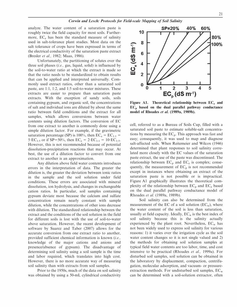
analyze. The water content of a saturation paste is

roughly twice the field capacity for most soils. Further-

more, ECe has been the standard measure of salinity

used in salt-tolerance plant studies. Most data on the

salt tolerance of crops have been expressed in terms of

the electrical conductivity of the saturation paste extract

(Bresler et al., 1982; Maas, 1986).

Unfortunately, the partitioning of solutes over the

three soil phases (i.e., gas, liquid, solid) is influenced by

the soil-to-water ratio at which the extract is made so

that the ratio needs to be standardized to obtain results

that can be applied and interpreted universally. Com-

monly used extract ratios, other than a saturated soil

paste, are 1:1, 1:2, and 1:5 soil-to-water mixtures. These

extracts are easier to prepare than saturation paste

extracts. With the exception of sandy soils, soils

containing gypsum, and organic soil, the concentrations

of salt and individual ions are diluted by about the same

ratio between field conditions and the extract for all

samples, which allows conversions between water

contents using dilution factors. The conversion of EC

from one extract to another is commonly done using a

simple dilution factor. For example, if the gravimetric

saturation percentage (SP) is 100%, then ECe 5 EC1:1 5

5?EC1:5 or if SP550%, then ECe 5 2?EC1:1 5 10?EC1:5.

However, this is not recommended because of potential

dissolution-precipitation reactions that may occur. At

best, the use of a dilution factor to convert from one

extract to another is an approximation.

Any dilution above field water contents introduces

errors in the interpretation of data. The greater the

dilution is, the greater the deviation between ionic ratios

in the sample and the soil solution under field

conditions. These errors are associated with mineral

dissolution, ion hydrolysis, and changes in exchangeable

cation ratios. In particular, soil samples containing

gypsum deviate most because the calcium and sulfate

concentration remain nearly constant with sample

dilution, while the concentrations of other ions decrease

with dilution. The standardized relationship between the

extract and the conditions of the soil solution in the field

for different soils is lost with the use of soil-to-water

above saturation. However, the recent development of

software by Suarez and Taber (2007) allows for the

accurate conversion from one extract ratio to another,

provided sufficient chemical information is known (i.e.,

knowledge of the major cations and anions and

presence/absence of gypsum). The disadvantage of

determining soil salinity using a soil sample is the time

and labor required, which translates into high cost.

However, there is no more accurate way of measuring

soil salinity than with extracts from soil samples.

Prior to the 1950s, much of the data on soil salinity

was obtained by using a 50-mL cylindrical conductivity

cell, referred to as a Bureau of Soils Cup, filled with a

saturated soil paste to estimate soluble-salt concentra-

tions by measuring the ECp. This approach was fast and

easy; consequently, it was used to map and diagnose

salt-affected soils. When Reitemeier and Wilcox (1946)

determined that plant responses to soil salinity corre-

lated more closely with the EC values of the saturation

paste extract, the use of the paste was discontinued. The

relationship between ECp and ECe is complex; conse-

quently, the measurement of ECp is not recommended

except in instances where obtaining an extract of the

saturation paste is not possible or is impractical.

Figure A1 graphically illustrates the theoretical com-

plexity of the relationship between ECp and ECe based

on the dual parallel pathway conductance model of

Rhoades et al. (1989a, 1989b).

Soil salinity can also be determined from the

measurement of the EC of a soil solution (ECw), where

the water content of the soil is less than saturation,

usually at field capacity. Ideally, ECw is the best index of

soil salinity because this is the salinity actually

experienced by the plant root. Nevertheless, ECw has

not been widely used to express soil salinity for various

reasons: 1) it varies over the irrigation cycle as the soil

water content changes so it is not single valued and 2)

the methods for obtaining soil solution samples at

typical field water contents are too labor, time, and cost

intensive to be practical (Rhoades et al., 1999a). For

disturbed soil samples, soil solution can be obtained in

the laboratory by displacement, compaction, centrifu-

gation, molecular adsorption, and vacuum- or pressure-

extraction methods. For undisturbed soil samples, ECw

can be determined with a soil-solution extractor, often

Figure A1. Theoretical relationship between ECe and

ECp based on the dual parallel pathway conductance

model of Rhoades et al. (1989a, 1989b).

21

Corwin and Lesch: Protocols for Field-scale Mapping of Soil Salinity

referred to as a porous cup extractor, or using an in situ,

imbibing-type porous-matrix salinity sensor.

There are various advantages and disadvantages

to measuring EC using soil solution extractors or soil

salinity sensors. The obvious advantage is that ECw is

being measured, but this is outweighed by the disad-

vantages. Even though the sample volume of a soil-

solution extractor (i.e., 10–100 cm3) is roughly an order

of magnitude larger than a salinity sensor (i.e., 1–2 cm3),

both measure very limited sample volumes; consequent-

ly, there are serious doubts about the ability of soil

solution extractors and porous-matrix salinity sensors to

provide representative soil water samples, particularly at

field scales (England, 1974; Raulund-Rasmussen, 1989;

Smith et al., 1990). Soil heterogeneity significantly

affects chemical concentrations in the soil solution.

Because of their small sphere of measurement, both

solution extractors and salt sensors do not adequately

integrate spatial variability (Amoozegar-Fard et al.,

1982; Haines et al., 1982; Hart and Lowery, 1997).

Biggar and Nielsen (1976) suggested that soil solution

samples are ‘‘point samples’’ that can provide a good

qualitative measurement of soil solutions, but not

adequate quantitative measurements unless the field-scale

variability is adequately established. Furthermore, salinity

sensors demonstrate a response time lag that is dependent

upon the diffusion of ions between the soil solution and

solution in the porous ceramic, which is affected by 1) the

thickness of the ceramic conductivity cell, 2) the diffusion

coefficients in soil and ceramic, and 3) the fraction of the

ceramic surface in contact with soil (Wesseling and Oster,

1976). The salinity sensor is generally considered the least

desirable method for measuring ECw because of its low

sample volume, unstable calibration over time, and slow

response time (Corwin, 2002). Soil solution extractors

have the drawback of requiring considerable maintenance

because of cracks in the vacuum lines and clogging of the

ceramic cups with algae and fine soil particles. Both

solution extractors and salt sensors are considered slow

and labor intensive.

The ability to obtain the EC of a soil solution when

the water content is at or less than field capacity, which are

the water contents most commonly found in the field, is

considerably more difficult than extracts for water contents

at or above saturation because of the pressure or suction

required to remove the soil solution at field capacity and

lower water contents. The EC of the saturated paste is the

easiest to obtain followed by the EC of extracts greater

than SP, followed by the EC of extracts less than SP.

However, it is ECe above all others that is most preferred;

consequently, either measuring ECe or being able to relate

the EC measurement to ECe is critical.

Because of the time and cost of obtaining soil

solution extracts and the lag time associated with porous

ceramic cups, developments in the measurement of soil

EC shifted in the 1970s to the measurement of the soil

electrical conductivity of the bulk soil, referred to as

apparent soil electrical conductivity (ECa). Apparent

soil electrical conductivity provides an immediate, easy-

to-take measurement of conductance with no lag time

and no need to obtain a soil extract. Furthermore, ECa

can be related to ECe. However, ECa is a complex

measurement that has been misinterpreted and misun-

derstood by users in the past because of the fact that it is a

measure of the electrical conductance of the bulk soil and

not just a measure of the conductance of the soil solution,

which is the desired measurement since the soil solution is

the soil phase that contains the salts affecting plant roots.

The techniques of ER, EMI, and TDR measure ECa. The

most comprehensive body of research concerning the

adaptation and application of geophysical techniques to

the measurement of soil salinity within the root zone (top

1 to 1.5 m of soil) was compiled by scientists at the U.S.

Salinity Laboratory. The most recent reviews of this body

of research can be found in Rhoades et al. (1999a, 1999b),

Corwin (2005), and Corwin and Lesch (2005a).

Electrical Resistivity

Electrical resistivity was originally used by geo-

physicists to measure the resistivity of the geological

subsurface. Electrical resistivity methods involve the

measurement of the resistance to current flow across

four electrodes inserted in a straight line on the soil

surface at a specified distance between the electrodes

(Corwin and Hendrickx, 2002). The electrodes are

connected to a resistance meter that measures the

potential gradient between the current and potential

electrodes (Fig. A2). These four-electrode methods were

developed in the second decade of the 1900s by Conrad

Schlumberger in France and Frank Wenner in the USA

for the evaluation of near-surface ER (Rhoades and

Halvorson, 1977; Burger, 1992).

Even though two electrodes (one current and one

potential electrode) can be used, the stability of the

reading is greatly improved with the use of four

electrodes. With two electrodes, measurements are

obscured or even masked by electrode polarization,

which happens because of the interaction of the charged

electrode surface with free charges in the electrolyte

forming an electrical double layer on the electrode

surface with a large capacitance. The factors affecting

the double layer thickness are electrolyte concentration,

valency, and electrode design. Four-electrode measure-

ment techniques mitigated the problem of electrode

polarization by providing a second pair of electrodes to

measure the voltage across the soil.

The resistance is converted to EC using Eq. (A3),

where the cell constant, k, in Eq. (A3) is determined by

22

Journal of Environmental and Engineering Geophysics

the electrode configuration and distance. The depth of

penetration of the electrical current and the volume of

measurement depends on the electrode configuration

and spacing between the electrodes. The two most

common electrode configurations are the Wenner array

and the Schluberger array. The four electrodes for the

Wenner array are equidistantly spaced (inter-electrode

spacing 5 a). For a homogeneous soil, the depth of

penetration of the Wenner array is approximately equal

to 1.5a and the soil volume measured is roughly equal to

pa3. Whereas, for the Schlumberger array the two inner

potential electrodes are fixed and spaced closer together

than the distance from inner to outer electrodes. The

depth of penetration of the electrical current and the

volume of measurement increases as the distance

between the potential and current electrodes increases

for both the Wenner and Schlumberger arrays.

There are additional four-electrode configurations

that are frequently used, as discussed by Burger (1992),

Telford et al. (1990), and Dobrin (1960). The influence

of the inter-electrode configuration and distance on ECa

is reflected in Eq. (A4):

ECa,25oC~1000

2pRt

� �ft

1

1

r1{

1

r2{

1

R1z

1

R2

8>>>>>><>>>>>>:

9>>>>>>=>>>>>>;ðA4Þ

where ECa,25oC is the apparent soil electrical conductivity

temperature corrected to a reference of 25uC (dS m21)

and r1, r2, R1, and R2 are the distances in cm between the

electrodes as shown in Fig. A2. For the Wenner array,

where a 5 r1 5 r2 5 R1 5 R2, Eq. (A4) reduces to ECa 5

159.2 ft/aRt and 159.2/a represents the cell constant (k).

Electrical resistivity is a technique that requires

good contact between the soil and four electrodes

inserted into the soil; consequently, it produces less

reliable measurements in dry or stony soils than EMI,

which does not require physical contact with the soil.

Nevertheless, ER has a flexibility that has proven

advantageous for field application, i.e., the depth and

volume of measurement can be easily changed by

altering the spacing between the electrodes. A distinct

advantage of the ER approach is that the volume of

measurement is determined by the spacing between the

electrodes, which makes a large volume of measurement

possible. For example, a 1-m inter-electrode spacing for

a Wenner array results in a volume of measurement of

more than 3 m3. This large volume of measurement

integrates the high level of local-scale variability often

associated with ECa measurements.

Because ECe is regarded as the standard measure

of salinity, a relation between ECa and ECe is needed to

relate ECa to salinity. The relationship between ECa and

ECe is linear when ECa is above 2 dS m21 and is

dependent on soil texture as shown in Fig. A3. Rough

approximations of ECe from ECa in dS m21 when ECa

$ 2 dS m21 are: ECe < 3.5 ? ECa for fine-textured soils,

ECe < 5.5 ? ECa for medium-textured soils, and ECe <7.5 ? ECa for coarse-textured soils. For ECa , 2 dS m21

the relation between ECa and ECe is more complex. In

general, at ECa $ 2 dS m21 salinity is the dominant

conductive constituent; consequently, the relationship

between ECa and ECe is linear. However, when ECa ,

2 dS m21 other conductive properties (e.g., water and

clay content) and properties influencing conductance

(e.g., bulk density) have greater influence. For this

reason, it is recommended that below an ECa of 2 dS m21

the relation between ECa and ECe is established by

calibration. The calibration between ECa and ECe is

established by measuring the ECe of soil samples taken

at a minimum of 3–4 locations within a study area where

associated ECa measurements have been taken. These

samples should reflect a range of ECas and should be

collected over the volume of measurement for the ECa

technology used (i.e., ER or EMI).

Electromagnetic Induction

Electromagnetic induction consists of a transmit-

ter coil located at one end of the EMI instrument that

induces circular eddy-current loops in the soil with the

magnitude of these loops directly proportional to the

electrical conductivity in the vicinity of that loop. Each

current loop generates a secondary electromagnetic field

that is proportional to the value of the current flowing

within the loop. A fraction of the secondary induced

electromagnetic field from each loop is intercepted by

the receiver coil of the instrument and the sum of these

signals is amplified and formed into an output voltage,

which is related to a depth-weighted ECa. The amplitude

and phase of the secondary field will differ from those of

the primary field as a result of soil properties (e.g., clay

content, water content, salinity), spacing of the coils and

Figure A2. Schematic of four-electrode probe electrical

resistivity used to measure apparent soil electrical con-

ductivity (Corwin and Hendrickx, 2002).

23

Corwin and Lesch: Protocols for Field-scale Mapping of Soil Salinity

their orientation, frequency, and distance from the soil

surface (Hendrickx and Kachanoski, 2002).

The most commonly used EMI conductivity

meters in soil science and in vadose zone hydrology

are the Geonics2 EM31 and EM38 and the DUALEM-

23. The EM38 has had considerably greater application

for agricultural purposes because the depth of measure-

ment corresponds roughly to the root zone (i.e.,

generally 1 to 1.5 m.). When the instrument is placed

in the vertical coil configuration (EMv, i.e., coils are

perpendicular to the soil surface) the depth of measure-

ment is about 1.5 m and in the horizontal coil

configuration (EMh, i.e., coils are parallel to the soil

surface), the depth of the measurement is 0.75–1.0 m.

The EM31 has an inter-coil spacing of 3.66 m, which

corresponds to a penetration depth of 3 and 6 m in the

horizontal and vertical dipole orientations, respectively,

which extends well beyond the root zone of agricultural

crops. However, the EM38 has one major pitfall, which

is the need for calibration, which the DUALEM-2 does

not require. Further details about and operation of the

EM31 and EM38 equipment are discussed in Hendrickx

and Kachanoski (2002). Documents concerning the

DUALEM-2 can be found online at http://www.

dualem.com/documents.html (verified 27 Sept. 2012).

Apparent soil electrical conductivity measured by

EMI at ECa , 1.0 dS m21 is given by Eq. (A5) from

McNeill (1980),

ECa{4

2pm0fs2

Hs

Hp

� �ðA5Þ

where ECa is measured in S m21; Hp and Hs are the

intensities of the primary and secondary magnetic fields

at the receiver coil (A m21), respectively; f is the

frequency of the current (Hz); m0 is the magnetic

permeability of air (4p1027 H m21); and s is the inter-

coil spacing (m).

Both ER and EMI are rapid and reliable

technologies for the measurement of ECa, each with its

advantage and disadvantage. The primary advantage of

EMI over ER is that EMI does not require physical

contact with the soil, so it can be used on dry and stony

soils that would not be amenable to ER equipment. The

primary advantage of ER over EMI is the ease of

instrument calibration. Calibrating the EM31 and

EM38 is more involved than for ER equipment.

However, as previously mentioned there is no need to

calibrate the DUALEM-2.

Profiling of soil ECa at various depth increments

using ER is a straightforward calculation and process.

For example, discrete depth intervals of soil ECa can be

determined with the Wenner array by measuring the

ECa of successive layers by increasing the inter-electrode

spacing from ai-1 to ai and using Eq. (A6) from Barnes

(1952) for resistors in parallel:

ECx~ECai{ai{1{

(ECai:ai){(ECai{1

{ai{1)

(ai{ai{1)ðA6Þ

where ai is the inter-electrode spacing, which equals the

depth of sampling and ai-1 is the previous inter-electrode

spacing, which equals the depth of previous sampling.

Unlike ER, profiling of ECa using EMI, though theo-

retically possible, is complex (Rhoades and Corwin 1981;

Corwin and Rhoades, 1982; Rhoades et al., 1990; Borchers

et al., 1997; Hendrickx et al., 2002; Morris, 2009) and has

resulted in limited application for this purpose.

Because of the different response functions of ER

and EMI instruments with depth, a comparison of ECa

measurements taken for the same volume of soil will not

be the same except by coincidence.

Time Domain Reflectometry

Time domain reflectometry (TDR) was initially

adapted for use in measuring water content, h (Topp et

al., 1980, 1982; Topp and Davis, 1981). The TDR

technique is based on the time for a voltage pulse to

travel down a soil probe and back, which is a function of

the dielectric constant (e) of the porous media being

2Geonics Limited, Mississauga, Ontario, Canada. Productidentification is provided solely for the benefit of the readerand does not imply the endorsement of the USDA.

3DUALEM Inc., Milton, Ontario, Canada. Product iden-tification is provided solely for the benefit of the reader anddoes not imply the endorsement of the USDA.

Figure A3. Relationships between ECa and ECe for

representative soil types found in the northern Great

Plains, USA. Modified from Rhoades and Halvorson

(1977).

24

Journal of Environmental and Engineering Geophysics

measured. Later, Dalton et al. (1984) demonstrated theutility of TDR to also measure ECa. The measurement

of ECa with TDR is based on the attenuation of the

applied signal voltage as it traverses the medium of

interest with the relative magnitude of energy loss

related to ECa (Wraith, 2002).

By measuring e, h can be determined through

calibration (Dalton, 1992). The e is calculated with Eq.

(A7) from Topp et al. (1980),

e~ct

2l

� �2

~la

lvp

� �2

ðA7Þ

where c is the propagation velocity of an electromag-

netic wave in free space (2.997 3 108 m s21), t is the

travel time (s), l is the real length of the soil probe (m), lais the apparent length (m) as measured by a cable tester,and vp is the relative velocity setting of the instrument.

The relationship between h and e is approximately linear

and is influenced by soil type, rb, clay content, and

organic matter (Jacobsen and Schjønning, 1993).

By measuring the resistive load impedance across

the probe (ZL), ECa can be calculated with Eq. (A8)

from Giese and Tiemann (1975),

ECa~e0c

l: Z0

ZLðA8Þ

where e0 is the permittivity of free space (8.854 3

10212 F m21), Z0 is the probe impedance (V), and ZL 5

Zu[(2V0/Vf)-1]21 where Zu is the characteristic imped-

ance of the cable tester, V0 is the voltage of the pulsegenerator or zero-reference voltage, and Vf is the final

reflected voltage at a very long time. To reference ECa to

25uC, Eq. (A9) is used:

ECa~KcftZ{1L ðA9Þ

where Kc is the TDR probe cell constant (Kc [m21] 5

e0cZ0/l), which is determined empirically.

Advantages of TDR for measuring ECa include: 1)

a relatively noninvasive nature since there is only minor

interference with soil processes, 2) an ability to measure

both soil water content and ECa, 3) an ability to detect

small changes in ECa under representative soil condi-

tions, 4) the capability of obtaining continuous unat-

tended measurements, and 5) a lack of a calibration

requirement for soil water content measurements in

many cases (Wraith, 2002). Even so, TDR has not been

the instrument of choice for the measurement of salinity,

whether in the laboratory or in the field; consequently, it

will not be discussed in detail.

Soil ECa has become one of the most reliable and

frequently used measurements to characterize field

variability for application to precision agriculture be-

cause of its ease of measurement and reliability (Corwin

and Lesch, 2003). Although TDR has been demonstrated

to compare closely with other accepted methods of ECa

measurement (Heimovaara et al., 1995; Mallants et al.,

1996; Spaans and Baker, 1993; Reece ,1998), it is still not

sufficiently simple, robust or fast enough for the general

needs of field-scale soil salinity assessment (Rhoades et

al., 1999b). Only ER and EMI have been adapted for the

geo-referenced measurement of ECa at field-scales and

larger (Rhoades et al., 1999a, 1999b).

25

Corwin and Lesch: Protocols for Field-scale Mapping of Soil Salinity