EOSC 512 2019

3 (More on) The Stress Tensor and the Navier-Stokes Equations

3.1 The symmetry of the stress tensor

In principle, the stress tensor has nine independent components. BUT only six of these are independent. That is

because the o↵-diagonal elements (those representing tangent or shear stresses as opposed to normal stresses) must

satisfy a symmetry condition, �ij = �ji. That is,

�12 = �21

�23 = �32

�13 = �31

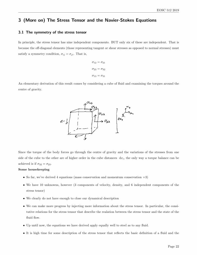
An elementary derivation of this result comes by considering a cube of fluid and examining the torques around the

centre of gravity.

Since the torque of the body forces go through the centre of gravity and the variations of the stresses from one

side of the cube to the other are of higher order in the cube distances dxi, the only way a torque balance can be

achieved is if �32 = �23.

Some housekeeping

• So far, we’ve derived 4 equations (mass conservation and momentum conservation ⇥3)

• We have 10 unknowns, however (3 components of velocity, density, and 6 independent components of the

stress tensor)

• We clearly do not have enough to close our dynamical description

• We can make more progress by injecting more information about the stress tensor. In particular, the consi-

tutive relations for the stress tensor that describe the realation between the stress tensor and the state of the

fluid flow.

• Up until now, the equations we have derived apply equally well to steel as to any fluid.

• It is high time for some description of the stress tensor that reflects the basic definition of a fluid and the

Page 22

EOSC 512 2019

properties of fluids like water and air that are of principal interest to us...

3.2 Putting the stress tensor in diagonal form

A key step in formulating the equations of motion for a fluid requires specifying the stress tensor in terms of the

properties of the flow (and in particular the velocity field) so that the theory becomes closed. That is, the number

of variables is reduced to the number of governing equations.

A key step towards this aim is to recognize that because the stress tensor is symmetric, we can always find a

coordinate frame in which the stresses are purely normal (where the stress tensor is diagonal).

Aside: In practice, finding this frame amounts to diagonalizing the

stress tensor �ij (which in the geographical x�y�z frame is generally

not diagonal to begin with). This is done by finding a transformation

matrix aij which renders �ij diagonal in a new frame. This exercise

yields an eigenvalue problem for the �j in the diagonalized tensor

and defines three eigenvalues corresponding to the three diagonal el-

ements of the new stress tensor. For each eigenvalue, there will be

an eigenvector. Sine the stress tensor is symmetric, the eigenvectors

corresponding to di↵erent eigenvalues are orthogonal and define the

coordinate frame in which � is diagonal (purely normal stresses).

We won’t review this diagonalization exercise here, although it is a

standard topic in most introductory linear algenbra courses if you

want a refresher.

Instead, we will move on secure in the knowledge that because the stress tensor is symmetric (�ij = �ji) we can

always find a frame in which the stress tensor is diagonal,

�ij =

0

BBB@

�1 0 0

0 �2 0

0 0 �3

1

CCCA(3.1)

3.3 A bit of an aside... The static (or hydrostatic) pressure and the deviatoric stress

Recall that one definition of a fluid is a material that, if subject to forces or stresses that will not lead to a change

of volume, deforms at a constant rate and so will not remain at rest.

In follows that in a fluid at rest, the stress tensor must have only diagonal terms. Further, the stress tensor would

have to be diagonal in any coordinate frame because the fluid doesn’t know which frame we choose to use to describe

the stress tensor.

The only 2nd order stress tensor that is diagonal in all frames is one in which each diagonal element is the same.

We define that value as the static pressure P (sometimes called the hydrostatic pressure – this is the pressure in a

Page 23

EOSC 512 2019

fluid at rest). In this case, the stress tensor is:

�ij = �P �ij = �P

0

BBB@

1 0 0

0 1 0

0 0 1

1

CCCA(3.2)

Where �ij is the Kronecker delta (�ij = 1 if i = j and �ij = 0 if i 6= j).

The fact that the stress tensor is isotropic implies that the normal stress in any orientation is always �P , and the

tangential stress is always zero (This isotropy of pressure is often called Pascal’s Law).

When the fluid is moving, the pressure (often defined as the average normal force on a fluid element) need not be

the thermodynamic pressure. That is,

�jj/3 =1

3(�11 + �22 + �33) (3.3)

Where �jj is the trace of the stress tensor (think back to Einstein notation!) and the RHS is the definition of

pressure in terms of the elements of the stress tensor for a moving fluid.

This definition is useful because the trace of the stress tensor �jj is invariant under coordinate transformations (As

you will show in an assignment!).

The deviatoric stress

We can always split the stress tensor into two parts and write it as:

�ij = �P �ij + ⌧ij (3.4)

Where ⌧ij (the deviatoric stress) is simply defined as the di↵erence between the pressure and the total stress tensor.

If We define the pressure as the average normal stress as above, then the race of the deviatoric stress tensor music

be zero (but if the pressure is so defined the we cannot guarantee it is equal to the thermodynamic pressure and

we will have to represent the di↵erence of the two also in terms of the fluid motion).

On the other hand, if we define the pressure as the thermodynamic pressure then the trace of ⌧ij 6= 0. Of course,

it is a matter of choice which of these we choose. The final equations will be the same.

3.4 The analysis of fluid motion at a point

We are next going to try to relate the stress tensor to some property of fluid motion. In almost all cases of interest

to us, this relationship will be a local one (This is an important property true for simple fluids).

Our approach will be to analyze the nature of the flow in the vicinity of an arbitrary point and discover what

aspects of the motion will determine the stress.

Consider the fluid motion near the point xi. Within a small neighbourhood of that point and using the continuous

nature of fluid motion we can represent the velocity in terms of a Taylor series. If the neighbourhood under con-

sideration is small, only the first term of this expansion is important.

ui(xj + �xj) = ui(xj) +@ui

@xj�xj (3.5)

Page 24

EOSC 512 2019

Where @ui@xj

is the deformation tensor and @ui@xj

�xj = �ui(xj) is the velocity deformation. Note that both the velocity

and the displacement �xi are vectors, so @ui@xj

is a second order tensor.

We can rewrite the velocity deviation as the sum of a symmetric tensor, �u(s)i and an antisymmetric part, �u(a)

i .

That is, �ui = �u(s)i + �u(a)

i , where:

�u(s)i = eij�xj =

1

2

✓@ui

@xj+

@uj

@xi

◆�xj (3.6)

�u(a)i = ⇠ij�xj

1

2

✓@ui

@xj�

@uj

@xi

◆�xj (3.7)

Where eij is the rate of strain tensor and ⇠ij is related to the vorticity.

3.5 The vorticity

Consider the antisymmetric part of the velocity deviation, ⇠ij�xj . ⇠ij has three components,0

@i = 2

j = 1

1

A ⇠21 =1

2

✓@u2

@x1�

@u1

@x2

◆= �⇠12

0

@i = 2

j = 1

1

A ⇠32 =1

2

✓@u3

@x2�

@u2

@x3

◆= �⇠23

0

@i = 1

j = 3

1

A ⇠13 =1

2

✓@u1

@x3�

@u3

@x1

◆= �⇠31

(3.8)

These are the three components of the vector 12~! = 1

2r⇥ ~u, where ! ⌘ curl(~u).

Or, in index notation, !i = "ijk@uk@xj

. We call "ijk the alternating tensor (Or Levi-Civita). "ijk = 1 if (i, j, k) is an

even permutation of (1, 2, 3), "ijk = �1 if (i, j, k) is an odd permutation of (1, 2, 3), and "ijk = 0 if any index is

repeated.

We call ~! ⌘ Vorticity. As we shall see, vorticity occupies a central place in the dynamics of atmospheric and oceanic

phenomena and it is one of the fundamental portions of the general composition of fluid motion.

The relationship between ⇠ij and the vorticity is fairly straightforward. For example, xi32 = !12 , with the other

fomponents following cycllically. In general,

⇠ij = �1

2"ijk!k (3.9)

The antisymmetric part of the velocity deviation �u(a)i is then

�u(a)i = ⇠ij�xj = �

1

2"ijk!k�xj = �

1

2"ikj!k�xj (3.10)

This may be more recognizable written in vector form,

�~u(a) =1

2~! ⇥ �~x (3.11)

Physically, �~u(a) represents the deviation velocity due to a pure rotation at a rotation rate which is one half the

local value of the vorticity. We recognize that it is a pure rotation because the associated velocity vector �~u(a) is

always perpendicular to the displacement �~x so there is no increase in the length of �~x, only a change in direction.

Page 25

EOSC 512 2019

3.6 The rate of strain tensor

Now consider the contribution of the symmetric part of the velocity deviation, eij =12

⇣@ui@xj

+ @uj

@xi

⌘�xj . This is the

rate of strain tensor.

To see the connection to the rate of strain, consider two di↵erential line element vectors, �~x and �~x0, originating at

the some point separated by angle ✓. The their respective lengths be �s and �s0:

Now, assuming the common origin is following the fluid, the each displacement vector will change depending on

changes in the di↵erence between the position of the origin and the position of the tip of the vector.

d

dt�xi = �ui (3.12)

Now consider the inner product of our two displacement vectors, �xi�x0i = �s�s0 cos ✓. The time rate of change of

this inner product is then:

d

dt�xi�x

0i =

d

dt(�s�s0 cos ✓)

=

✓�s

d

dt�s0 + �s0

d

dt�s

◆cos ✓ � sin ✓

d✓

dt�s�s0

(3.13)

We can also write ddt�xi�x0

i = �xi�u0i + �x0

i�ui (by applying product rule). By substituting �u0i = @ui

@xj�x0

j and

�ui =@ui@xj

�xj ,

d

dt�xi�x

0i = �xi

@ui

@xj�x0

j + �x0i@ui

@xj�xj interchanging dummy indices i and j in the last term

= �xi�xj

✓@ui

@xj+

@uj

@xi

◆

= 2eij�xi�x0j

(3.14)

Equating the RHS of equation 3.13 and equation 3.14 and dividing by �s�s0 (since we assume neither is singular)

yields:

cos ✓

✓1

�s0d

dt�s0 +

1

�s

d

dt�s

◆� sin ✓

d✓

dt= 2eij

�xi

�s

�x0j

�s0(3.15)

Page 26

EOSC 512 2019

Where �xi�s and

�x0j

�s0 are unit vectors in the directions of �~x and �~x0. We can use this equation to interpret the

components of the tensor eij

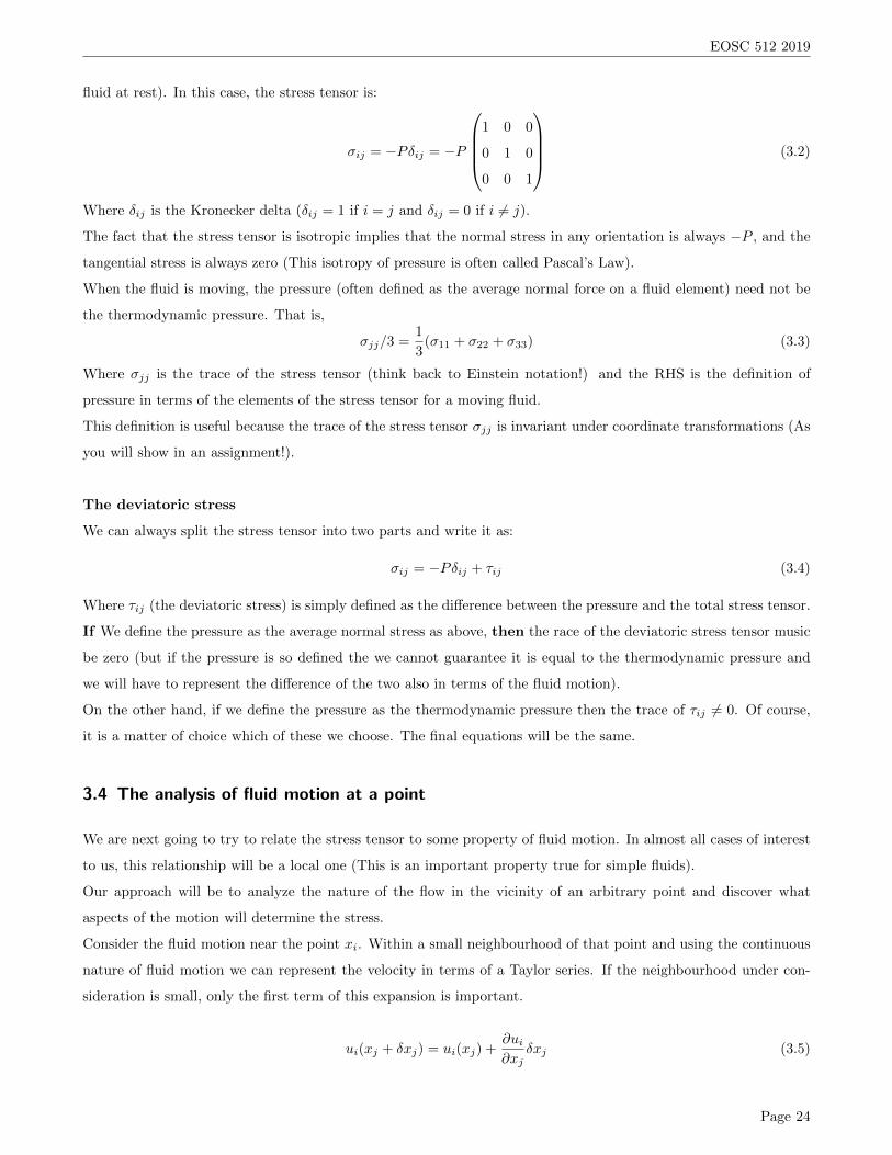
Example 3.1. Let �~x and �~x0 be colinear so that ✓ = 0 and let �~x lie along the x1 axis, �~x = (�x1, 0, 0).

If ✓ = 0, then cos ✓ = 1, sin ✓ = 1, and �s = �x1. Equation 3.15 then implies:

1

�x01

d

dt�x0

1 +1

�x1

d

dt�x1 (3.16)

If we take �x1 and �x01 to be the same length,

1

�x1

d

dt�x1 = e11 (3.17)

Physically, the diagonal elements of the rate of strain tensor represent the rate of stretching of a fluid element

along the corresponding axis.

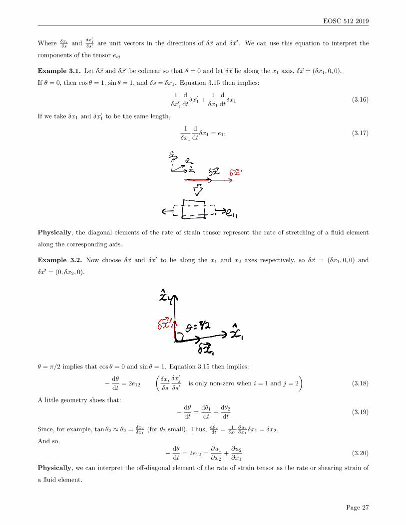
Example 3.2. Now choose �~x and �~x0 to lie along the x1 and x2 axes respectively, so �~x = (�x1, 0, 0) and

�~x0 = (0, �x2, 0).

✓ = ⇡/2 implies that cos ✓ = 0 and sin ✓ = 1. Equation 3.15 then implies:

�d✓

dt= 2e12

✓�xi

�s

�x0j

�s0is only non-zero when i = 1 and j = 2

◆(3.18)

A little geometry shoes that:

�d✓

dt=

d✓1dt

+d✓2dt

(3.19)

Since, for example, tan ✓2 ⇡ ✓2 = �x2�x1

(for ✓2 small). Thus, d✓2dt = 1

�x1

@u2@x1

�x1 = �x2.

And so,

�d✓

dt= 2e12 =

@u1

@x2+

@u2

@x1(3.20)

Physically, we can interpret the o↵-diagonal element of the rate of strain tensor as the rate or shearing strain of

a fluid element.

Page 27

EOSC 512 2019

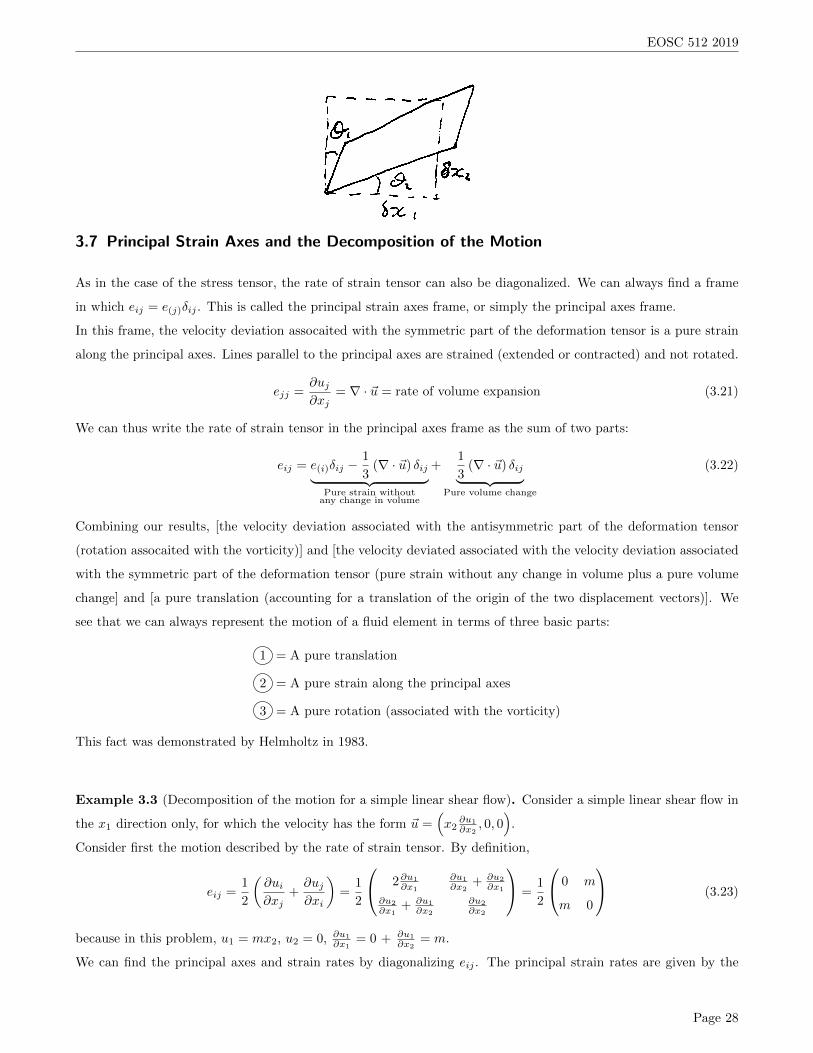
3.7 Principal Strain Axes and the Decomposition of the Motion

As in the case of the stress tensor, the rate of strain tensor can also be diagonalized. We can always find a frame

in which eij = e(j)�ij . This is called the principal strain axes frame, or simply the principal axes frame.

In this frame, the velocity deviation assocaited with the symmetric part of the deformation tensor is a pure strain

along the principal axes. Lines parallel to the principal axes are strained (extended or contracted) and not rotated.

ejj =@uj

@xj= r · ~u = rate of volume expansion (3.21)

We can thus write the rate of strain tensor in the principal axes frame as the sum of two parts:

eij = e(i)�ij �1

3(r · ~u) �ij

| {z }Pure strain withoutany change in volume

+1

3(r · ~u) �ij

| {z }Pure volume change

(3.22)

Combining our results, [the velocity deviation associated with the antisymmetric part of the deformation tensor

(rotation assocaited with the vorticity)] and [the velocity deviated associated with the velocity deviation associated

with the symmetric part of the deformation tensor (pure strain without any change in volume plus a pure volume

change] and [a pure translation (accounting for a translation of the origin of the two displacement vectors)]. We

see that we can always represent the motion of a fluid element in terms of three basic parts:

1 = A pure translation

2 = A pure strain along the principal axes

3 = A pure rotation (associated with the vorticity)

This fact was demonstrated by Helmholtz in 1983.

Example 3.3 (Decomposition of the motion for a simple linear shear flow). Consider a simple linear shear flow in

the x1 direction only, for which the velocity has the form ~u =⇣x2

@u1@x2

, 0, 0⌘.

Consider first the motion described by the rate of strain tensor. By definition,

eij =1

2

✓@ui

@xj+

@uj

@xi

◆=

1

2

0

@ 2@u1@x1

@u1@x2

+ @u2@x1

@u2@x1

+ @u1@x2

@u2@x2

1

A =1

2

0

@ 0 m

m 0

1

A (3.23)

because in this problem, u1 = mx2, u2 = 0, @u1@x1

= 0 + @u1@x2

= m.

We can find the principal axes and strain rates by diagonalizing eij . The principal strain rates are given by the

Page 28

EOSC 512 2019

eigenvalues e(j) roots of the characteristic equation defined by the condition for the vanishing determinant of the

2⇥ 2 matrix,

eij � e(j)I = 0������

0� e(j) 12m

12m 0� e(j)

������= 0

⇣e(j)

⌘2=

✓1

2m

◆2

= 0

e(j) = ±1

2m

(3.24)

So e(1) = + 12m and e(2) = �

12m. The are the principal strain rates (the elements of the rate of strain tensor in

diagonal form).

The principal axes are the eigenvectors (aj1, aj2)T that satisfy:

(eij � e(j))

0

@aj1

aj2

1

A = 0

0

@0� e(j) 12m

12m 0� e(j)

1

A

0

@aj1

aj2

1

A = 0

(3.25)

For e(1) = + 12m:

�1

2maj1 +

1

2maj2 = 0

�aj1 + aj2 = 0

Choose aj1 = aj2 =1p2

So the vector has unit length

(3.26)

The first eigenvector is any two element column vector in which the two elements have equal magnitude and sign.

For e(2) = �12m:

1

2maj1 +

1

2maj2 = 0

aj1 + aj2 = 0

aj1 = �aj2

Choose aj1 =1p2

and aj2 = �1p2

So the vector has unit length

(3.27)

The second eigenvector is any two element column vector in which the two element have equal magnitude and

opposite sign.

Thus, the principal axes are defined by the orthogonal eigenvectors 12 (1, 1)

T and 12 (1,�1)T. The rate of strain along

these axis directions is given by the eigenvalues e(1) and e(2), equal to + 12m and �

12m, respectively.

Page 29

EOSC 512 2019

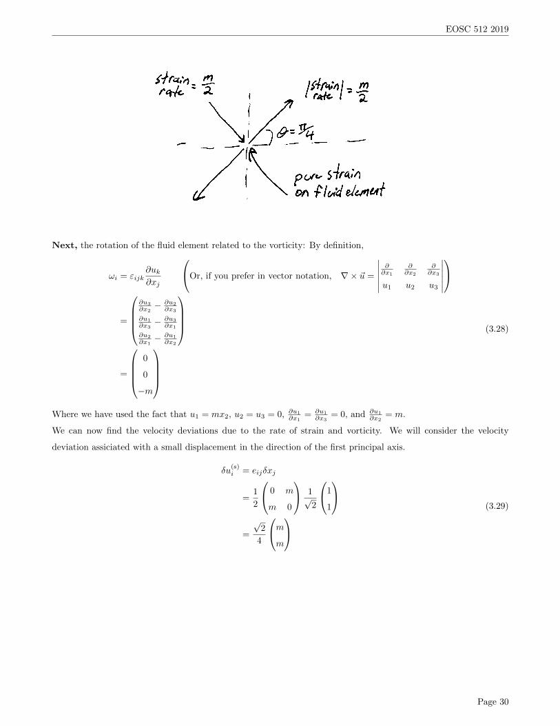
Next, the rotation of the fluid element related to the vorticity: By definition,

!i = "ijk@uk

@xj

0

@Or, if you prefer in vector notation, r⇥ ~u =

������

@@x1

@@x2

@@x3

u1 u2 u3

������

1

A

=

0

BBB@

@u3@x2

�@u2@x3

@u1@x3

�@u3@x1

@u2@x1

�@u1@x2

1

CCCA

=

0

BBB@

0

0

�m

1

CCCA

(3.28)

Where we have used the fact that u1 = mx2, u2 = u3 = 0, @u1@x1

= @u1@x3

= 0, and @u1@x2

= m.

We can now find the velocity deviations due to the rate of strain and vorticity. We will consider the velocity

deviation assiciated with a small displacement in the direction of the first principal axis.

�u(s)i = eij�xj

=1

2

0

@ 0 m

m 0

1

A 1p2

0

@1

1

1

A

=

p2

4

0

@m

m

1

A

(3.29)

Page 30

EOSC 512 2019

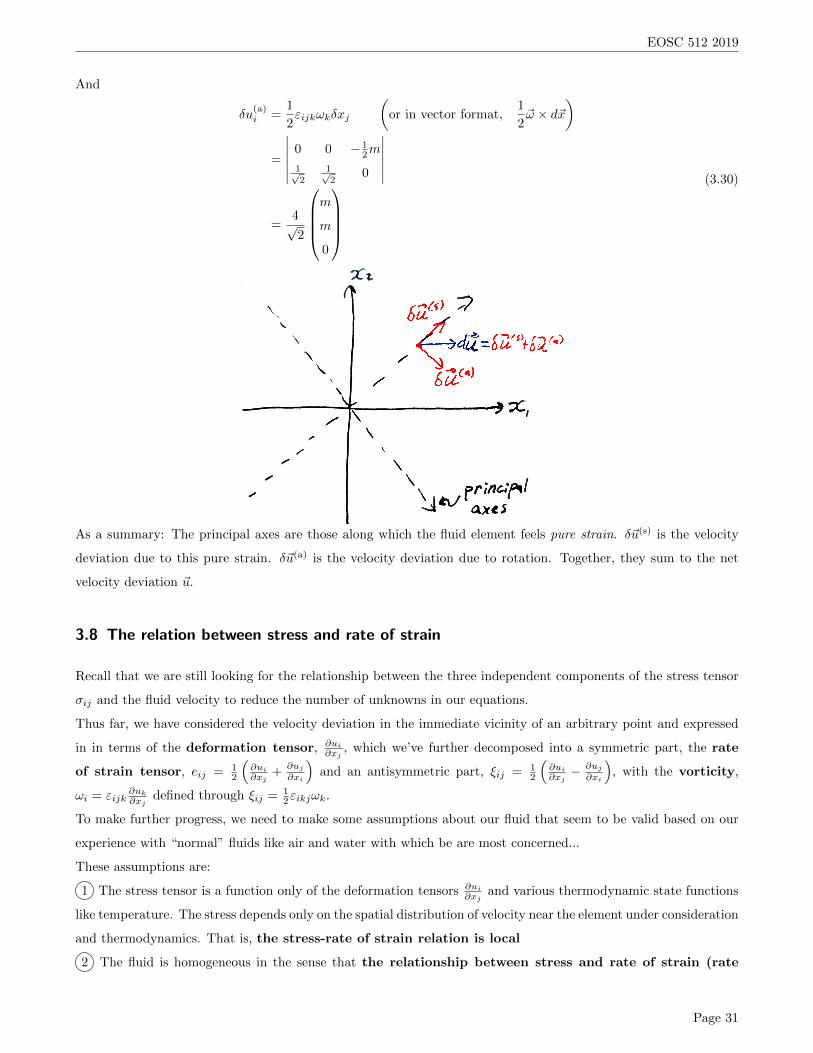
And

�u(a)i =

1

2"ijk!k�xj

✓or in vector format,

1

2~! ⇥ d~x

◆

=

������

0 0 �12m

1p2

1p2

0

������

=4p2

0

BBB@

m

m

0

1

CCCA

(3.30)

As a summary: The principal axes are those along which the fluid element feels pure strain. �~u(s) is the velocity

deviation due to this pure strain. �~u(a) is the velocity deviation due to rotation. Together, they sum to the net

velocity deviation ~u.

3.8 The relation between stress and rate of strain

Recall that we are still looking for the relationship between the three independent components of the stress tensor

�ij and the fluid velocity to reduce the number of unknowns in our equations.

Thus far, we have considered the velocity deviation in the immediate vicinity of an arbitrary point and expressed

in in terms of the deformation tensor, @ui@xj

, which we’ve further decomposed into a symmetric part, the rate

of strain tensor, eij = 12

⇣@ui@xj

+ @uj

@xi

⌘and an antisymmetric part, ⇠ij = 1

2

⇣@ui@xj

�@uj

@xi

⌘, with the vorticity,

!i = "ijk@uk@xj

defined through ⇠ij =12"ikj!k.

To make further progress, we need to make some assumptions about our fluid that seem to be valid based on our

experience with “normal” fluids like air and water with which be are most concerned...

These assumptions are:

1 The stress tensor is a function only of the deformation tensors @ui@xj

and various thermodynamic state functions

like temperature. The stress depends only on the spatial distribution of velocity near the element under consideration

and thermodynamics. That is, the stress-rate of strain relation is local

2 The fluid is homogeneous in the sense that the relationship between stress and rate of strain (rate

Page 31

EOSC 512 2019

of change of deformation) is the same everywhere. There is spatial variation in the stress �ij only due to

spatial variations on the deformation tensor @ui@xj

. (This distinguishes a fluid from a solid, for which the stress tensor

depends on the strain itself.)

3 The fluid is isotropic. The relation between stress and rate of strain has no preferred spatial orientation.

Obviously, given a particular rate of strain, as in the previous example, there will be a special direction for the

stress. But this is only because of the geometry of the strain field and not because of the structure of the fluid.

This is not true for certain fluids with long chain molecules in their structures for which rates of strain along the

direction of the chains give stresses di↵erent than in other directions.

Aside:

Assumptions 1 , 2 , and 3 collectively define what is called a

Stokesian Fluid (after George Gabriel Stokes). One important prop-

erty of a Stokesian Fluid is that the principal axes of the stress and

the principal axes of strain must coincide.

4 The relationship between stress and rate of strain is linear. This assumptions defines a Newtonian

fluid. A Newtonian fluid is one in which the viscous stresses arising from its flow, at every point, are linearly

proportional to the local rate of strain. Water and air satisfy this assumption. Ketchup and toothpaste don’t!

If assumptions 1 through 4 are satisfied, it implies we are searching for a general relation between the de-

viatoric stress and the deformation tensor of the form:

⌧ij = Tijkl@uk

@xl(3.31)

Wher Tijkl is a 4th order proportionality tensor that satisfies the conditions of homogeneity and isotropy. This

implies that Tijkl is independent of orientation in space, and any spatial structure to stress must reflect the spatial

structure of the deformation.

One can show that this most general 4th order isotropic tensor has the form:

Tijkl = ↵�ij�kl + �(�ik�jl + �il�jk) (3.32)

(One can also appreciate the evasion of this derivation... Ask if you want to see the proof, or trust blindly!)

From this, it follows that the stress tensor has the form:

�ij = �P �ij + ⌧ij

= �P �ij + (↵�ij�kl + �(�ik�jl + �il�jk))@uk

@xl

= �P �ij + ↵�ij@uk

@xk+ �

✓@ui

@xj+

@uj

@ui

◆(3.33)

The traditional notation uses � for ↵ and µ for �, so it is common to write the stress tensor as:

�ij = �P �ij + 2µeij + �ekk�ij (3.34)

Page 32

EOSC 512 2019

This is the stress tensor defined in terms of pressure and the rate of strain tensor which is valid for a fluid that

satisfies a local stress-rate of strain relation⇣

1⌘, is homogeneous

⇣2⌘, is isotropic

⇣3⌘, and has a linear

stress-rate of strain relation⇣

4⌘.

Some notes to keep in mind:

• The stress tensor depends on P and eij but not on the vorticity/antisymmetric part of the deformation tensor.

• The 3rd term, �ekk�ij , is proportional to the divergence of the velocity field (ekk = @uk@xk

when thinking

of Einstein notation). Recall that the divergence is related to the rate of volume change. If the fluid is

incompressible (which water is on the scale of ocean motions, for example), then this term is zero. Even if

the fluid is compressible (like air) in dynamics of interest, the deviatoric stress is important when the shear is

large (usually near boundaries) and typically dominates this relatively small divergence term

Back to the definition of P: Equation 3.34 Says that the stress tensor �ij depends on three scalars: P , µ, and

�. As we have discussed, there are two obvious definitions of P that need not be the same: The average normal

stress and the thermodynaic pressure.

If we define P as the average normal stress (momentarily we will label this as P ), then

P = P = �1

3�ii =

1

3(�11 + �22 + �33) (3.35)

This is a mechanical definition of pressure. It implies that the trace of the deviatoric stress must be zero:

Tr(⌧ij) = ⌧ii = 2µeii + �ekk�ii

= ejj(2µ+ 3�) (by swapping dummy indices)

= 0

(3.36)

This implies a relation between � and µ,

� = �2

3µ (3.37)

But at the end of the day, we will have to write out equations in a way that links the mechanics and thermodynamics,

and we will want to introduce the equilibrium thermodynamic pressure Pe.

P and Pe will di↵er by an amount depending on the normal stresses of deformation tensor that arise from the fluid’s

motion. More precisely, in an isotropic medium, the di↵erence between the two definitions of pressure is:

P = Pe � ⌘@ui

@xj�ij = Pe � ⌘ [dvujxj ] = Pe � ⌘r · ~u (3.38)

So the stress tensor in terms of the thermodynamic pressure becomes:

�ij = Pe�ij + 2µeij + (⌘ � 2/3µ)ekk�ij (3.39)

Of course, if we defined P as the thermodynamic in equation 3.34 we would have arrived at the result:

�ij = Pe�ij + 2µeij + �ekk�ij (3.40)

(So the relation between the two formulations tells us � = ⌘ � 2/3µ.)

Page 33

EOSC 512 2019

Some notes:

• P and Pe di↵er when the fluid is composed of complex molecules with internal degrees of freedom. In this

case, the stress can also depend on the rate at which the fluid density is changing with time.

• We see this dependence as a contribution to the pressure in the form ⌘(r · ~u) where r · ~u is a measure of

the rate of density change (it represents the rate of change of the fluid volume per unit volume as seen by an

observer moving with the fluid).

• For the fluid of interest to us, ⌘ can be quite large: Approximated 3µ for water and 100µ for air at STP. But

the e↵ect on the flow of this term involving ⌘ and r · ~u is usually small even in compressible flows. This is

true except when density changes over vary small distances (in shockwaves) or very short timescales (high

intensity ultrasound).

• In “practical” GFD, it is common to take ⌘ = 0 and neglect this term,

�ij = �Pe�ij + 2µeij + �ekk�ij (3.41)

where � = �2/3µ.

• This form of the stress tensor was derived first by the fluid dynamicist Claude-Louis Navier in 1822 without

the divergence terms. Other derivations followed by Cauchy (1828), Poisson (1829), Saint-Venant (1843), and

finally a form more closely resembling the above by Stokes (1845). The resulting fluid momentum equations

with the full stress tensor in this form are called the Navier-Stokes equations.

3.9 The Navier-Stokes Equations

Now that we have an explicit form for the stress tensor in terms of the pressure and the fluid velocity (specifically

the spatial gradient of the fluid velocity in the form of the deformation tensors), we can write the momentum

equation in a form suitable for a fluid. Using equation 3.41 and substituting into the momentum equation 2.33, we

get:

⇢Dui

Dt= ⇢Fi �

@P

@xi+

@

@xj(2µeij) +

@

@xi

✓�@uk

@xk

◆(3.42)

Or equivalently, by expanding eij in terms of the velocity gradients:

⇢Dui

Dt= ⇢Fi �

@P

@xi+

@

@xj

✓µ

✓@ui

@xj+

@uj

@xi

◆◆+

@

@xi

✓�@uk

@xk

◆(3.43)

These are the full Navier-Stokes equations in index notation! Here (and henceforth) we have dropped the subscript

e on the pressure and we are assuming P is the thermodynamic pressure and not the average normal stress. As

they stand, it is di�cult to write these equations completely in vector form, but with some notational looseness,

⇢D~u

Dt= ⇢~F �rP + µr2 + (�+ µ)r (r · ~u) + (r�) (r · ~u) + ii2eij

@u

@xj(3.44)

Page 34

EOSC 512 2019

Which, if the fluid is incompressible and and if the temperature variations in the fluid are small enough so the

viscosity can be approximated as a constant becomes the more familiar:

⇢D~u

Dt= �rP + ⇢~F + µr2~u (3.45)

Some housekeeping

• We currently have four equations (mass conservation and three momentum equations) and five unknowns. So

we are still one equation short. To resolve this, we would need a way to relate density to the pressure field. Or

in the simplest case, we could assume constant density. In all other cases, we will have to consider coupling

the dynamical equations we have derived to continuum statements of the laws of thermodynamics.

• Note that the total time derivative D~ut contains the nonlinear ~u ·r~u, which is awkward to express in other

coordinates (such as spherical coordinates, which is particularly relevant to describing fluid motions on a

rotating planet...)

• We use the identity ~u ·r~u = ~! ⇥ ~u+r|~u|2/2 to derive another form of the Navier-Stokes equations:

⇢

✓@u

@t+ ~! ⇥ ~u

◆= ⇢~F

⇣rP + ⇢r|~u|2/2

⌘+ µr2~u (3.46)

• Once again, note that the Navier-Stokes equations are nonlinear due to the advection of momentum by the

velocity field.

• It can also be helpful to note that if the fluid is incompressible, you can show that the frictional force µr2~u

can be witten as �µr⇥ ~!. So you can express friction force in terms of the vorticity!

Page 35