Embed Size (px)
Citation preview

3He Injection Coils
Christopher Crawford, Genya Tsentalovich,
Wangzhi Zheng, Septimiu Balascuta,
Steve Williamson
nEDM Collaboration Meeting
2011-06-07
Injection beamline magnetic elements
4K shield
77K sheild
TR1a coil at 4K
TR1b coil at 77K
TR2a coil at 300K
TR2b coil at 300K
TR3a Helmholtz coils (outer TR3b
coils not in model)
trouble
regions
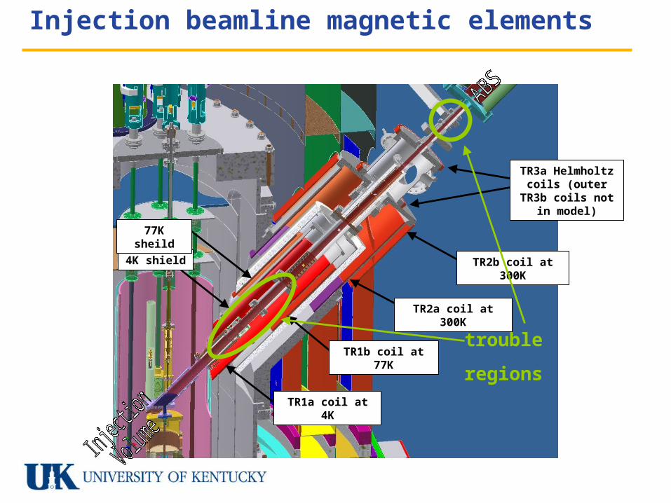
Previous spin precession simulations
Wangzhi Zheng
doubling the injection field improves to 95% polarization
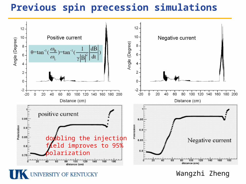
Old approach
PROBLEMS1. The magnetic field from ABS quadrupole on μ-metal shield is about 2G.2. The solenoidal field near the ABS exit is too small to preserve polarization.3. The field is less than Earth field outside the μ-metal shield (active shielding doesn’t shield the external fields).4. The direction of polarization is wrong before the entrance into cosθ coil.
ABS quadrupole
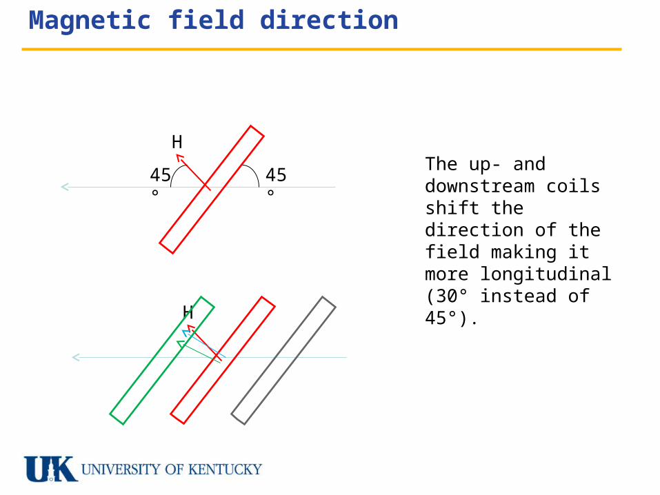
Magnetic field direction
H
45°
45°
H
The up- and downstream coils shift the direction of the field making it more longitudinal(30° instead of 45°).
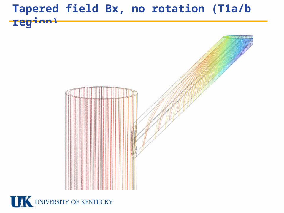
Tapered field Bx, no rotation (T1a/b region)
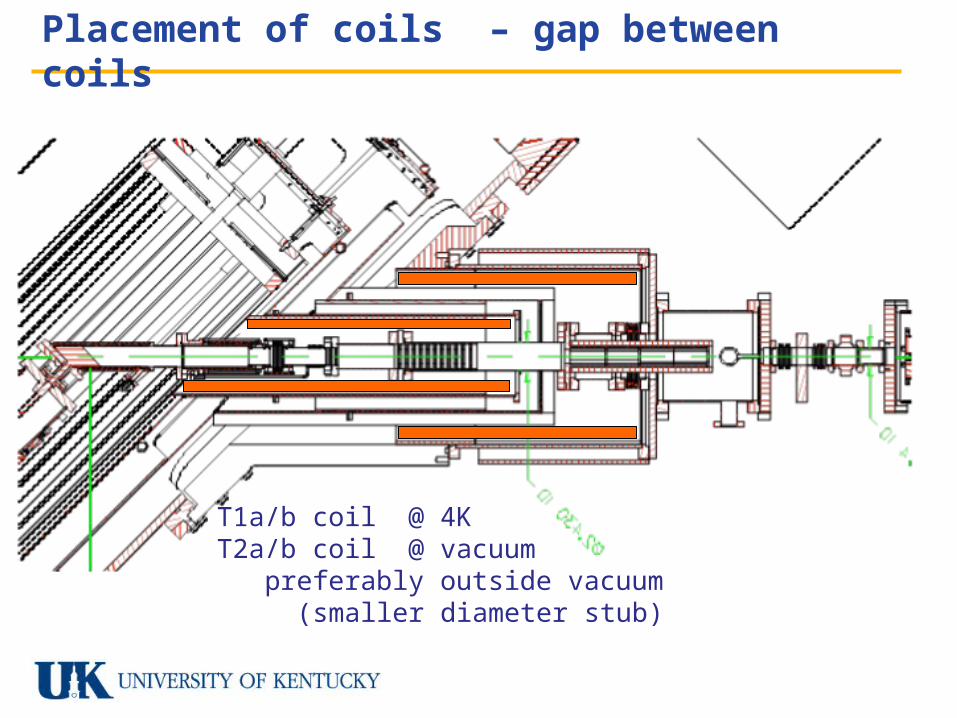
Placement of coils – gap between coils
T1a/b coil @ 4KT2a/b coil @ vacuum preferably outside vacuum (smaller diameter stub)
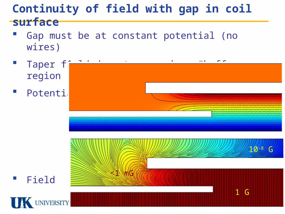
Continuity of field with gap in coil surface
Gap must be at constant potential (no wires)
Taper field down to zero in a “buffer region”
Potential
Field
1 G
<1 mG
10-8 G
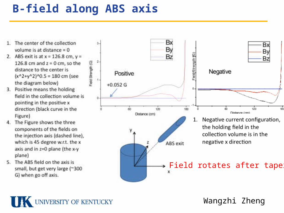
B-field along ABS axis
Field rotates after taper
Wangzhi Zheng
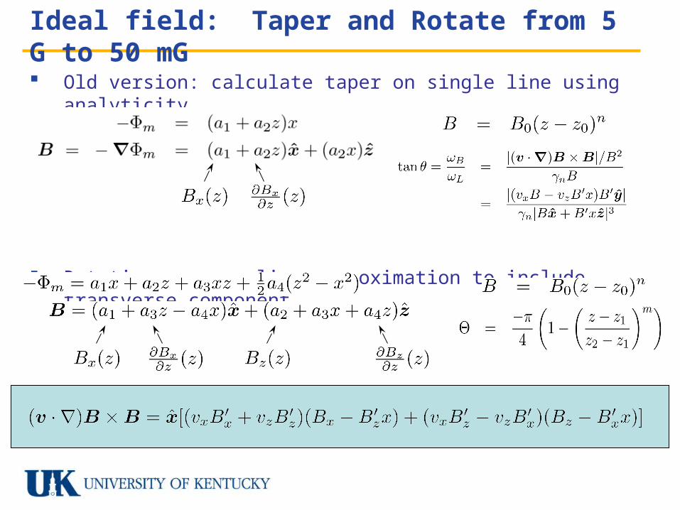
Ideal field: Taper and Rotate from 5 G to 50 mG
Old version: calculate taper on single line using analyticity
Rotation: generalize approximation to include transverse component
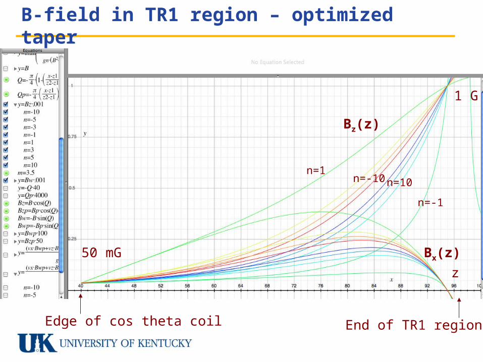
B-field in TR1 region – optimized taper
Edge of cos theta coil End of TR1 region
n=-1
n=1n=10n=-10
Bz(z)
z
Bx(z)50 mG
1 G
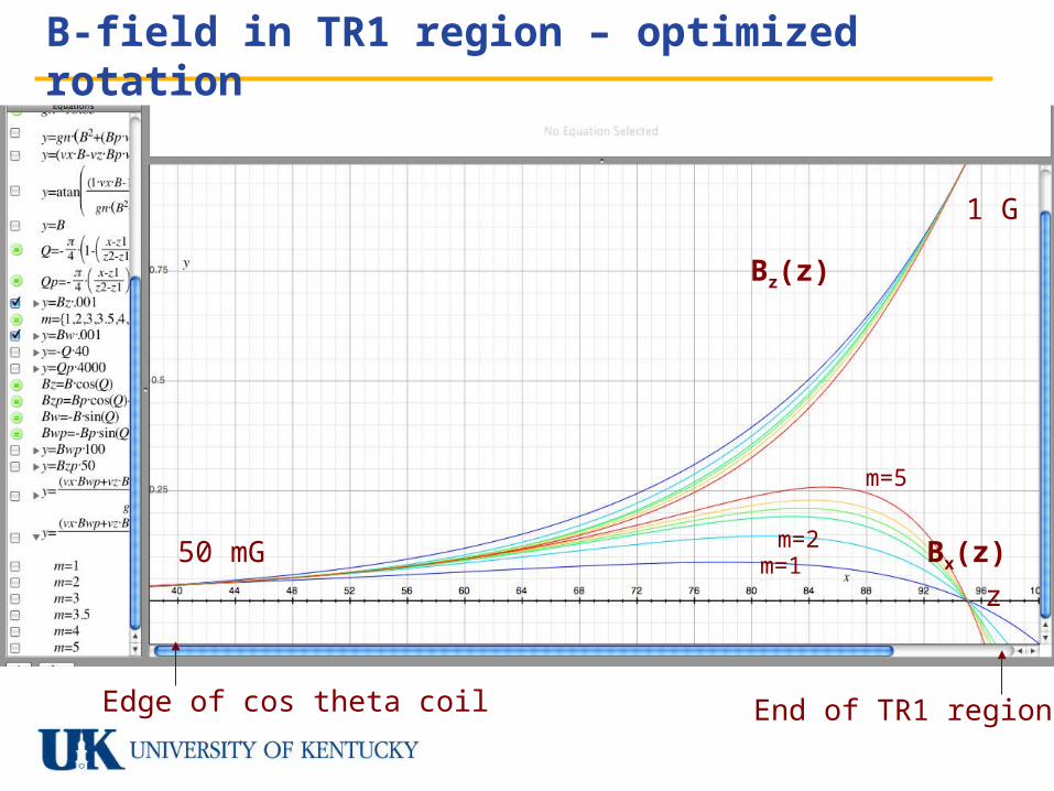
B-field in TR1 region – optimized rotation
1 G
Edge of cos theta coil End of TR1 region
m=5
m=1m=2
Bz(z)
z
Bx(z)50 mG
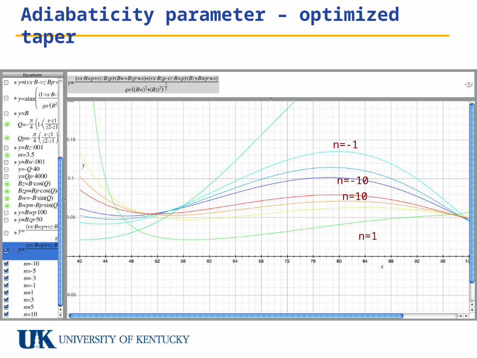
Adiabaticity parameter – optimized taper
n=-1
n=1
n=10
n=-10
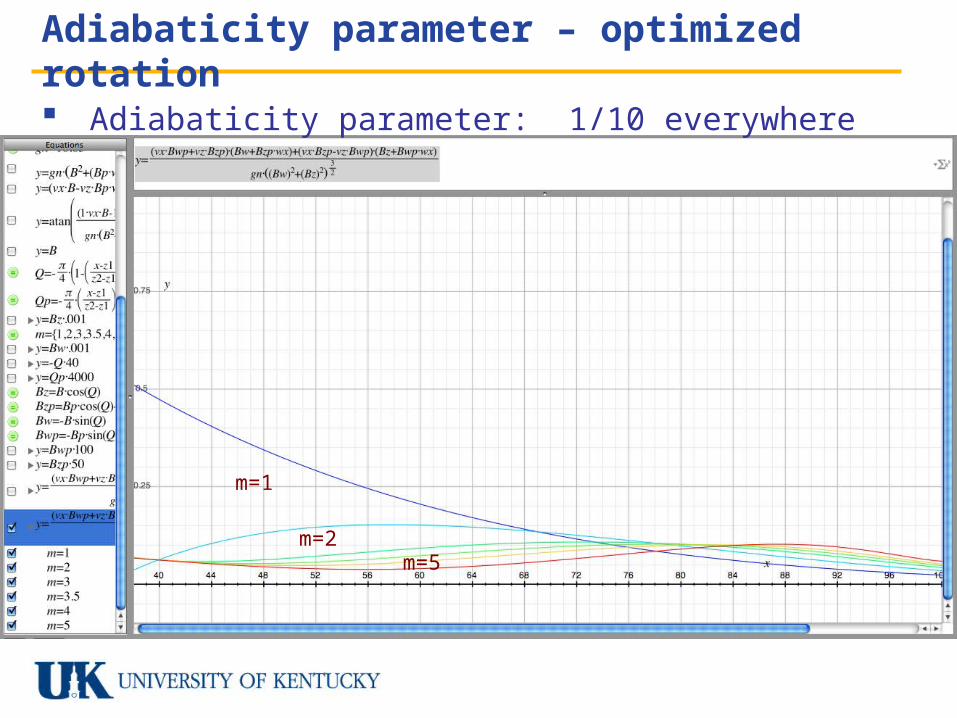
Adiabaticity parameter – optimized rotation
Adiabaticity parameter: 1/10 everywhere
m=5
m=1
m=2
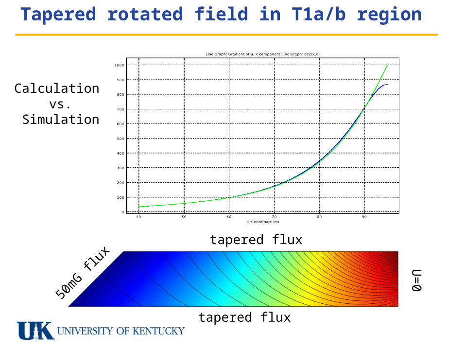
Tapered rotated field in T1a/b region
tapered flux
tapered flux
50m
G flux
U=
0
Calculation vs.
Simulation
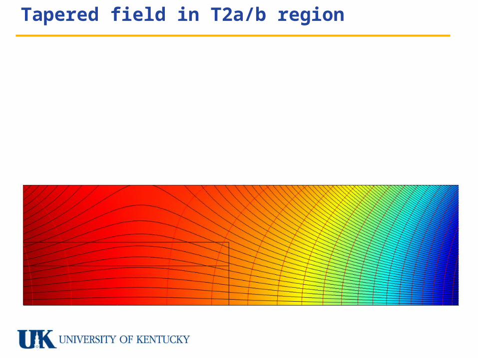
Tapered field in T2a/b region
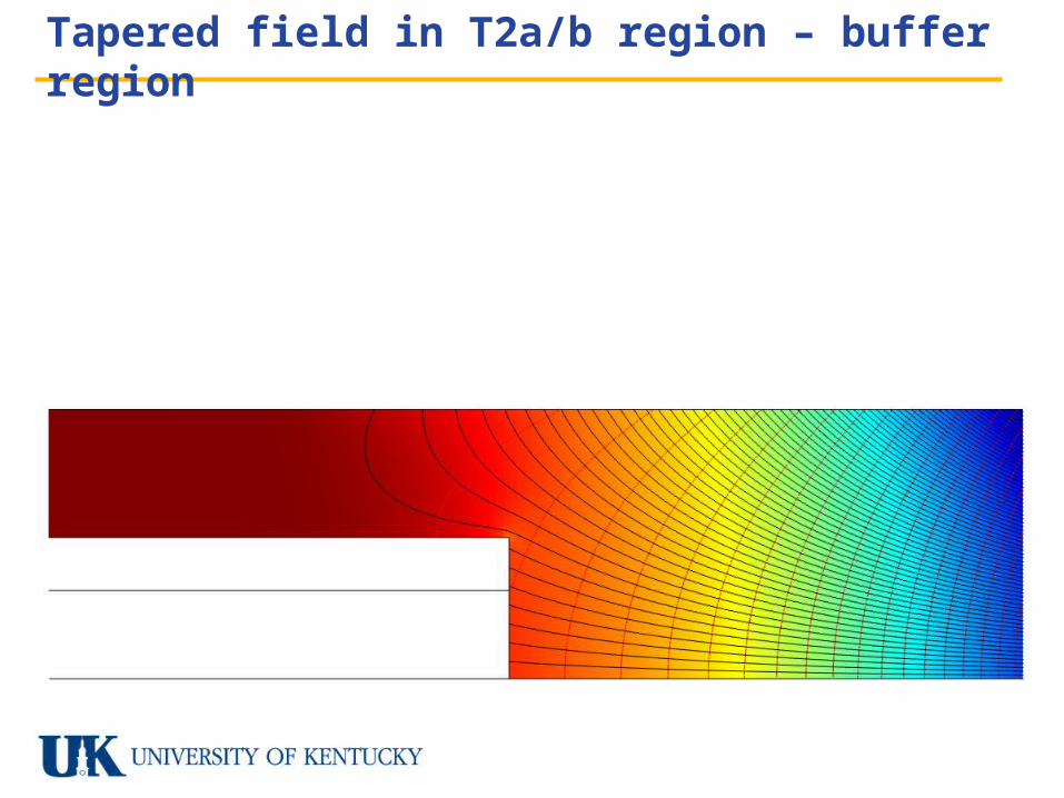
Tapered field in T2a/b region – buffer region
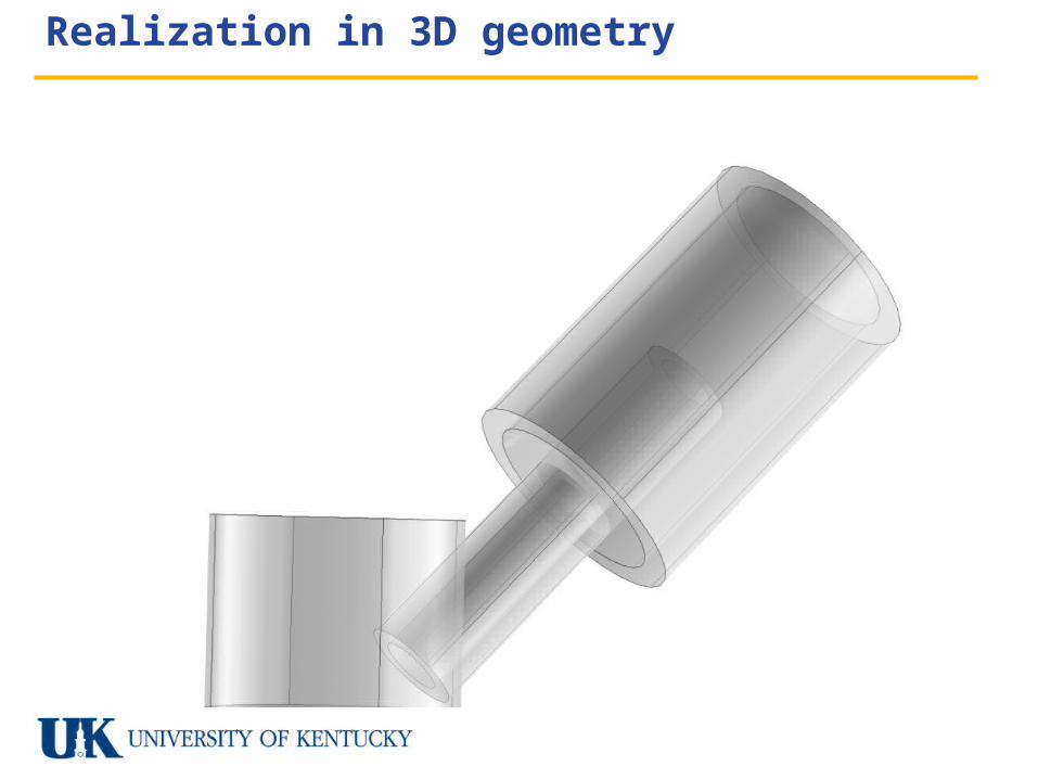
Realization in 3D geometry
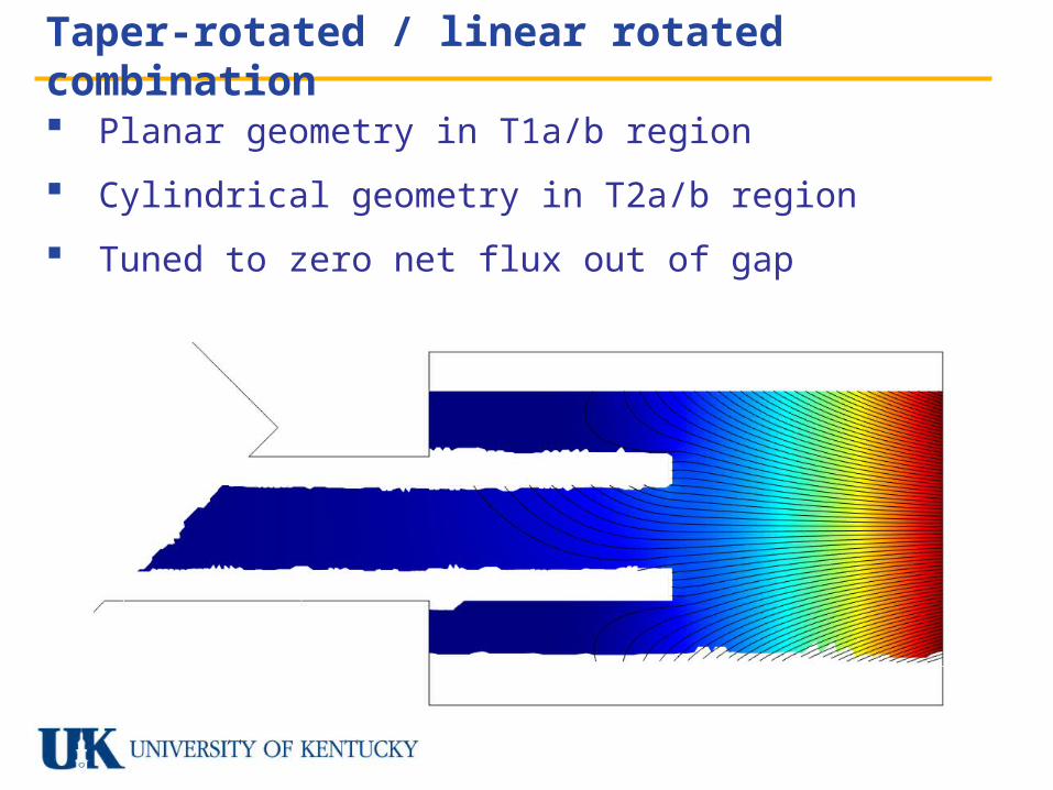
Taper-rotated / linear rotated combination
Planar geometry in T1a/b region
Cylindrical geometry in T2a/b region
Tuned to zero net flux out of gap
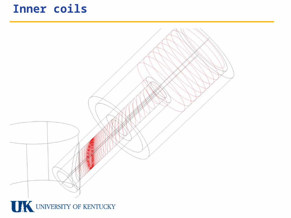
Inner coils
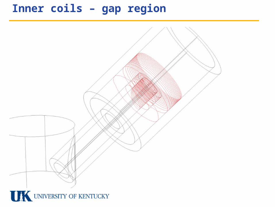
Inner coils – gap region
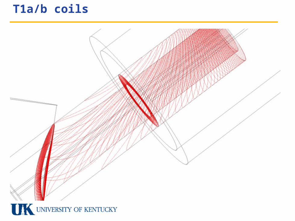
T1a/b coils
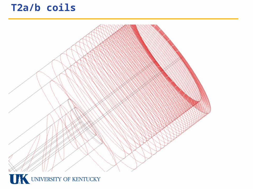
T2a/b coils
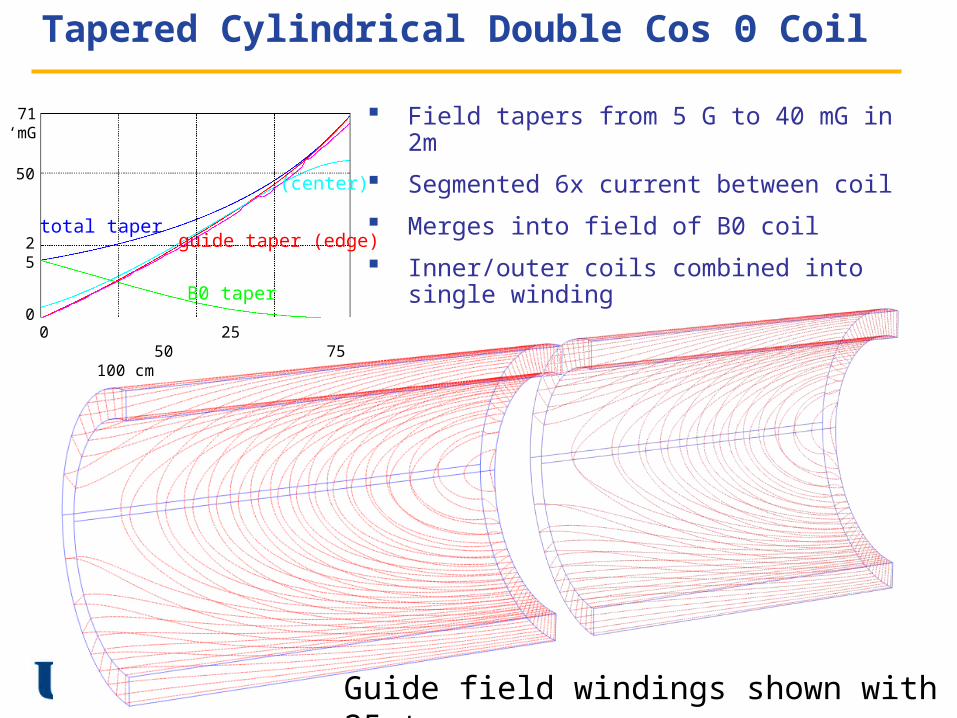
Tapered Cylindrical Double Cos Θ Coil
Field tapers from 5 G to 40 mG in 2m
Segmented 6x current between coil
Merges into field of B0 coil
Inner/outer coils combined intosingle winding
0 25 50 75 100 cm
0
25
50
71 ‘mG
total taper
B0 taper
guide taper (edge)
(center)
Guide field windings shown with 25 turns
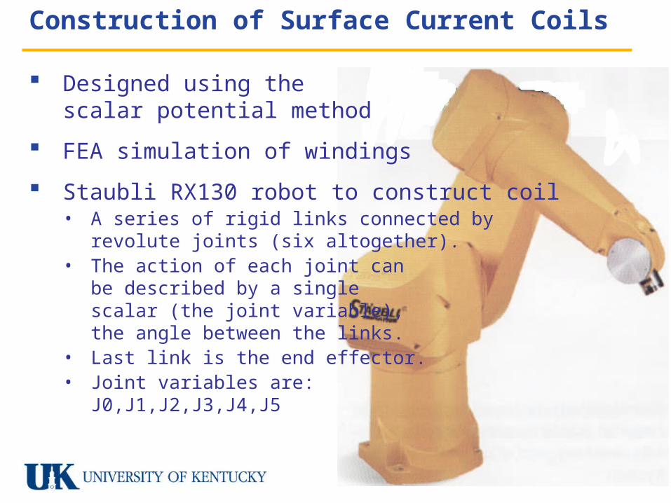
Construction of Surface Current Coils
Designed using thescalar potential method
FEA simulation of windings
Staubli RX130 robot to construct coil• A series of rigid links connected by
revolute joints (six altogether).• The action of each joint can
be described by a singlescalar (the joint variable),the angle between the links.
• Last link is the end effector.• Joint variables are:
J0,J1,J2,J3,J4,J5
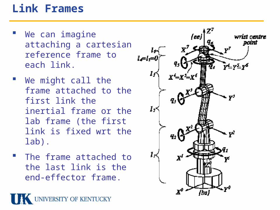
Link Frames
We can imagine attaching a cartesian reference frame to each link.
We might call the frame attached to the first link the inertial frame or the lab frame (the first link is fixed wrt the lab).
The frame attached to the last link is the end-effector frame.
Coordinate Transforms
Given the coordinates of a point in one frame, what are its coordinates in another frame?
The relationship between the end-effector frame and the inertial frame is of particular interest. (The location of the drill is fixed w/r the end-effector frame. The location of the electroplated form is fixed w/r the inertial frame).
Generally, six independent parameters are needed to relate one frame to another (3 to say where the second origin is, 3 to orient the second set of axes).
For the link frames, the position of each origin is flexible, so the relation can be specified with 4 parameters, one of which is the joint variable. These are the DH parameters.
DH Parameters / Homogeneous Transform Matrix
To repeat: the relationship between link frames can be characterized by 4 parameters, one of which is the joint variable. The other 3 are fixed, and relate to the size and placement of the links.
Using the fixed DH parameters and the joint variable, we can compute a transformation matrix needed to translate one link's coordinates into the adjacent link's coordinates.
T(J) is a 4x4 matrix of the following form:
i' j' k' T ( 0 0 0 1 )
We can compose transformations to relate any two frames.
Problem: Forward / Inverse Kinematics
With these concepts in place, we can address the following problem:
Given an actuation, determine the position and orientation (i.e., the pose) of some body fixed in the end-effector frame with respect to the inertial frame.
{J0, J1, J2, J3, J4, J5} -> {x, y, z, alpha, beta, gamma}
Solution: Build the transformation matrix for the given actuation and apply it to every point in the body. Alpha, beta and gamma can be compute directly from i', j’, k'.
Conversely:
Given a pose, find an actuation that will produce it.
Problem: Calibration
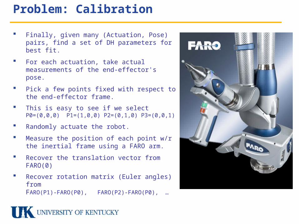
Finally, given many (Actuation, Pose) pairs, find a set of DH parameters for best fit.
For each actuation, take actual measurements of the end-effector's pose.
Pick a few points fixed with respect to the end-effector frame.
This is easy to see if we select P0=(0,0,0) P1=(1,0,0) P2=(0,1,0) P3=(0,0,1)
Randomly actuate the robot.
Measure the position of each point w/r the inertial frame using a FARO arm.
Recover the translation vector from FARO(0)
Recover rotation matrix (Euler angles) fromFARO(P1)-FARO(P0), FARO(P2)-FARO(P0), …
Positioning [Tooling]
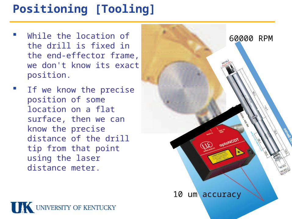
While the location of the drill is fixed in the end-effector frame, we don't know its exact position.
If we know the precise position of some location on a flat surface, then we can know the precise distance of the drill tip from that point using the laser distance meter.
60000 RPM
10 um accuracy
Geometry Capture/Wire Placement
Once the robot is calibrated (that is to say, we know the pose of its end effector for any actuation), we can capture the geometry of the electroplated form using the laser displacement meter.
Coil Design: [Magnetic Scalar Potential Technique]1. A digital representation of the form geometry.2. A description of the field we desire within the form.
Feed output of COMSOL back to robot to drill windings on the form
Conclusion
New techniques• Rotating fields• Gap between current surface
Converging on designs for guide fields• Neutron guide• 3He injection tube• 3He transfer region
Developing the capability to construct coils• Robotic arm with • laser displacement sensor• high speed spindle


![arxiv.org · arXiv:math/0608572v2 [math.RA] 9 Feb 2007 MORITA EQUIVALENCES INDUCED BY BIMODULES OVER HOPF-GALOIS EXTENSIONS STEFAAN CAENEPEEL, SEPTIMIU CRIVEI, ANDREI MARCUS, AND](https://img.pdfslide.us/doc/110x75/5e4bc978a2ae9505ba1100e4/arxivorg-arxivmath0608572v2-mathra-9-feb-2007-morita-equivalences-induced.jpg)