Embed Size (px)
Citation preview

Essays in Security Analysis and Trading
DISSERTATIONof the University of St.Gallen
School of Management,Economics, Law, Social Sciences
and International Affairsto obtain the title of
Doctor of Philosophy in Finance
Submitted by
Alexandru Septimiu Rif
from
Romania
Approved on the application of
Prof. Dr. Karl Frauendorfer
and
Prof. Dr. Marc Arnold
Dissertation no. 5013
Difo-Druck GmbH, Untersiemau 2020

The University of St.Gallen, School of Management, Economics, Law, SocialSciences and International Affairs hereby consents to the printing of thepresent dissertation, without hereby expressing any opinion on the viewsherein expressed.
St Gallen, May 25, 2020
The President:
Prof. Dr. Bernhard Ehrenzeller

Acknowledgements
I would like to extend my gratitude to a number of remarkable peoplethat have generously helped and guided me throughout my doctoral studies.
A special acknowledgment goes to Prof. Dr. Karl Frauendorfer, mysupervisor for his valuable support. I would like to thank my co-authors, Prof.Robert Gutsche, Ph.D. and Prof. Dr. Sebastian Utz for their collaborationand valuable insights. I would also like to thank my co-supervisors Prof. Dr.Marc Arnold and Prof. Dr. Angelo Ranaldo for their helpful comments andsuggestions. Furthermore, I would like to acknowledge the very helpful inputreceived during the PiF Seminars at the University of St Gallen.
Last but not least, I would like to thank my family and friends, who havealways offered me their unconditional support. Thank you!
St Gallen, January 2020
Alexandru Rif
i

Summary
This dissertation lies at the intersection of fundamental and technical in-vestment analysis. In their search for key market signals, which lie at thefoundation of investment decisions, both fundamental and technical investorsare faced with the challenging task of acquiring and interpreting financialdata, with the goal of extracting decision relevant information. Advancesin computation technology and data management systems have enabled thesurfacing of intra-day algorithmic traders, relying on their fast reaction timesand computational power to interpret market signals and identify key invest-ment and divestment signals. On the other hand, the fundamental investoruses financial statements as his primary source of information in order toidentify and assess a company’s individual value drivers.
Chapter I of this dissertation is devoted to investigating stock priceoverreactions around idiosyncratic crashes on the Nasdaq100. The scope ofthe analysis is to uncover whether liquidity provision after stock price crashesis beneficial for investors with short reaction times.
Chapter II investigates market conditions across individual exchangesin the case of cross-listed securities around a macro-economic event whichtriggered a concomitant three sigma negative return for 71 Nasdaq100 mem-bers. Specifically, this chapter looks into developments in liquidity, tradingcosts and trading activity across primary, secondary and tertiary exchanges.
Chapter III aims at analyzing the effect of segment reporting on ana-lysts’ earnings forecast accuracy. Particularly, it investigates the link betweenEPS forecast errors and the arising profitability “gap” when comparing prof-itability aggregated from segment reporting and firm profitability as derivedfrom consolidated financial statements.
ii

Zusammenfassung
Thematisch befindet sich diese Dissertation am Schnittpunkt fundamen-taler und technischer Investitionsanalyse. Auf der Suche nach wichtigenMarktsignalen und entscheidungsrelevanten Informationen stehen sowohl fun-damentale als auch technische Anleger vor der Herausforderung, Finanz-daten fur ihre Anlageentscheidungen erfassen und interpretieren zu konnen.Fortschritte in der Computertechnologie und in Datenverwaltungssystemenfuhren zum Einen dazu, dass im taglichen Handel vermehrt Algorithmenzur Interpretation relevanter Marktsignale und zur Identifikation transak-tionsauslosender Investitions- und Verausserungssignale Anwendung finden.Die Algorithmen zielen dabei insbesondere auf schnelle Reaktionszeiten undRechenleistung ab. Zum Anderen nutzt der fundamentale Investor den Ab-schluss als primare Informationsquelle, um die individuellen Werttreiber einesUnternehmens zu identifizieren und zu bewerten.
Kapitel I dieser Dissertation befasst sich mit der Untersuchung ubertrieb-ener Aktienkursreaktionen im Zusammenhang mit idiosynkratischen Kurs-sturzen von Nasdaq100-Unternehmen. Im Rahmen der Analyse soll herausge-funden werden, ob die Bereitstellung von Liquiditat nach einem Borsencrashfur Anleger mit kurzen Reaktionszeiten einen Vorteil bietet.
Kapitel II untersucht anhand 71 Nasdaq100-Unternehmen die Marktbe-dingungen fur auf einzelnen Borsen zweitkotierten Wertpapiere im Zusam-menhang mit makrookonomischen Ereignissen, die eine Drei-Sigma-Negativ-rendite auslosten. Dieses Kapitel befasst sich insbesondere mit der Entwick-lung der Liquiditat, der Handelskosten und der Handelsaktivitat an Primar-,Sekundar- und Tertiarborsen.
Kapitel III zielt darauf ab, die Auswirkungen der Segmentberichterstat-tung auf die Genauigkeit der Gewinnprognosen der Analysten zu analysieren.Insbesondere wird der Zusammenhang zwischen Gewinnerwartungen von An-alysten und den Rentabilitatsabweichungen untersucht, die entstehen, wenndie Segmentberichterstattung und nicht der konsolidierte Abschluss zu Prog-nosezwecken verwendet wird.
iii

Table of Contents
1 Acknowledgments . . . . . . . . . . . . . . . . . . . . . . . . . . . . . . . . . . . . . . . . . . . . . . . . . . . . . . . . i
2 Summary . . . . . . . . . . . . . . . . . . . . . . . . . . . . . . . . . . . . . . . . . . . . . . . . . . . . . . . . . . . . . . . ii
3 Zusammenfassung . . . . . . . . . . . . . . . . . . . . . . . . . . . . . . . . . . . . . . . . . . . . . . . . . . . . . . iii
4 Chapter I . . . . . . . . . . . . . . . . . . . . . . . . . . . . . . . . . . . . . . . . . . . . . . . . . . . . . . . . . . . . . . . 2
4.1 Introduction . . . . . . . . . . . . . . . . . . . . . . . . . . . . . . . . . . . . . . . . . . . . . . . . . . . . . . . .4
4.2 Data . . . . . . . . . . . . . . . . . . . . . . . . . . . . . . . . . . . . . . . . . . . . . . . . . . . . . . . . . . . . . . 10
4.3 Methodology and Results . . . . . . . . . . . . . . . . . . . . . . . . . . . . . . . . . . . . . . . . . .11
4.4 Conclusion . . . . . . . . . . . . . . . . . . . . . . . . . . . . . . . . . . . . . . . . . . . . . . . . . . . . . . . . 30
4.5 References . . . . . . . . . . . . . . . . . . . . . . . . . . . . . . . . . . . . . . . . . . . . . . . . . . . . . . . . 32
4.6 Appendix . . . . . . . . . . . . . . . . . . . . . . . . . . . . . . . . . . . . . . . . . . . . . . . . . . . . . . . . . 36
5 Chapter II . . . . . . . . . . . . . . . . . . . . . . . . . . . . . . . . . . . . . . . . . . . . . . . . . . . . . . . . . . . . . 39
5.1 Introduction . . . . . . . . . . . . . . . . . . . . . . . . . . . . . . . . . . . . . . . . . . . . . . . . . . . . . . 41
5.2 Theoretical Framework . . . . . . . . . . . . . . . . . . . . . . . . . . . . . . . . . . . . . . . . . . . . 45
5.3 Sample Selection and Data . . . . . . . . . . . . . . . . . . . . . . . . . . . . . . . . . . . . . . . . 49
5.4 Analysis and Main Results . . . . . . . . . . . . . . . . . . . . . . . . . . . . . . . . . . . . . . . . 57
5.5 Conclusion . . . . . . . . . . . . . . . . . . . . . . . . . . . . . . . . . . . . . . . . . . . . . . . . . . . . . . . . 70
5.6 References . . . . . . . . . . . . . . . . . . . . . . . . . . . . . . . . . . . . . . . . . . . . . . . . . . . . . . . . 71
5.7 Appendix . . . . . . . . . . . . . . . . . . . . . . . . . . . . . . . . . . . . . . . . . . . . . . . . . . . . . . . . . 75
6 Chapter III . . . . . . . . . . . . . . . . . . . . . . . . . . . . . . . . . . . . . . . . . . . . . . . . . . . . . . . . . . . . 84
6.1 Introduction . . . . . . . . . . . . . . . . . . . . . . . . . . . . . . . . . . . . . . . . . . . . . . . . . . . . . . 86
6.2 Background Literature and Hypothesis . . . . . . . . . . . . . . . . . . . . . . . . . . . . 88
6.3 Research Design . . . . . . . . . . . . . . . . . . . . . . . . . . . . . . . . . . . . . . . . . . . . . . . . . . . 95
6.4 Data . . . . . . . . . . . . . . . . . . . . . . . . . . . . . . . . . . . . . . . . . . . . . . . . . . . . . . . . . . . . . 100
6.5 Empirical Results . . . . . . . . . . . . . . . . . . . . . . . . . . . . . . . . . . . . . . . . . . . . . . . . 103
6.6 Conclusion . . . . . . . . . . . . . . . . . . . . . . . . . . . . . . . . . . . . . . . . . . . . . . . . . . . . . . . 116
6.7 References . . . . . . . . . . . . . . . . . . . . . . . . . . . . . . . . . . . . . . . . . . . . . . . . . . . . . . . 120
6.8 Appendix . . . . . . . . . . . . . . . . . . . . . . . . . . . . . . . . . . . . . . . . . . . . . . . . . . . . . . . . 126
7 Vita . . . . . . . . . . . . . . . . . . . . . . . . . . . . . . . . . . . . . . . . . . . . . . . . . . . . . . . . . . . . . . . . . . 130
1

Chapter IShort-term Stock Price Reversals after
Extreme Events
Alexandru Rif Sebastian Utz
Abstract
We studied the intraday effects of market fragmentation and returnoverreactions around stock price crashes of Nasdaq100 constituentsbased on nanosecond data. We analyzed whether market fragmenta-tion and liquidity provision after stock price crashes is beneficial forinvestors with short reaction time. We found that market fragmenta-tion does not affect the recovery after the crash which we documentto be at 31% of the negative one-minute crash interval return in thesubsequent trading minute. The relative magnitude of the reversalafter crash intervals was particularly high for the 20% most liquid andthe 20% smallest firms of our sample.
JEL classification: G12, G14, L11.
Keywords : Stock price reversal; High-frequency trading; Stock price crash;Market fragmentation.

List of Figures
1 . . . . . . . . . . . . . . . . . . . . . . . . . . . . . . . . . . . 6
2 . . . . . . . . . . . . . . . . . . . . . . . . . . . . . . . . . . . 7
3 . . . . . . . . . . . . . . . . . . . . . . . . . . . . . . . . . . . 8
4 . . . . . . . . . . . . . . . . . . . . . . . . . . . . . . . . . . . 17
List of Tables
1 . . . . . . . . . . . . . . . . . . . . . . . . . . . . . . . . . . . 15
2 . . . . . . . . . . . . . . . . . . . . . . . . . . . . . . . . . . . 20
3 . . . . . . . . . . . . . . . . . . . . . . . . . . . . . . . . . . . 23
4 . . . . . . . . . . . . . . . . . . . . . . . . . . . . . . . . . . . 25
5 . . . . . . . . . . . . . . . . . . . . . . . . . . . . . . . . . . . 28
6 . . . . . . . . . . . . . . . . . . . . . . . . . . . . . . . . . . . 29
7 . . . . . . . . . . . . . . . . . . . . . . . . . . . . . . . . . . . 36
8 . . . . . . . . . . . . . . . . . . . . . . . . . . . . . . . . . . . 37
9 . . . . . . . . . . . . . . . . . . . . . . . . . . . . . . . . . . . 38
3
1. Introduction
The rise of electronic, fully-automated markets resulted in an unprece-
dented increase in market fragmentation, triggering increased levels of at-
tention from regulators, investors and academic scholars alike. An ardent
discussion emerged on whether increased market fragmentation is beneficial
or detrimental to financial markets’ liquidity. Aitken et al. (2017) found that
market fragmentation is associated with improved market quality, while Up-
son and VanNess (2017) and Bessembinder (2003) argued that competition
between exchanges was linked with lower transaction costs and increased
liquidity. These studies primarily investigate the effects of market fragmen-
tation in normal trading conditions, while the role of market fragmentation
in times of extreme intraday events, remains an open empirical question.
In market microstructure literature, a vivid discussion emerged on the
question of whether a new type of investors, so-called high frequency traders
(HFTs) provide or detract liquidity on financial markets. HFTs are defined
as ‘professional traders acting in proprietary capacity’ who use ‘extraordi-
narily high-speed and sophisticated computer programs for generating, rout-
ing, and executing orders’ by the U.S. Securities and Exchange Commission
(SEC). The rise of electronic markets, increased computing power, algorith-
mic trading and reduced latency have been the primary enabling factors for
the emergence of HFTs. Concerning van Kervel and Menkveld (2019), Kora-
jczyk and Murphy (2018), HFTs acted as market makers in a normal market
environment (i.e., provided liquidity), but traded in line with the market per-
ception (i.e., detracted liquidity) as soon as they detected a persistent trend.
However, the general literature on the impact of HFTs on bid-ask spreads
and price efficiency, as well as their contribution to extreme market move-
ments such as the flash crash is mixed. While Hasbrouck and Saar (2013),
Chaboud et al. (2014), Hasbrouck (2018) documented a negative correlation
between HFT and crashes, Gao and Mizrach (2016), Boehmer et al. (2018),
Kirilenko et al. (2017) showed an increased frequency of crashes related to
4

HFT activities.
This paper investigates short-term price movements in the context of
stocks with various degrees of market fragmentation. At least two types of
events exist that can trigger large price movements: an update in information
and imbalances of trades. While the information contained in news updates
results in a rapid adjustment of prices on efficient markets, imbalances of
trades push prices away from fundamental values. In recent times, the emer-
gence of extreme transitory price movements, such as the flash crash on May
3, 2010, have attracted significant attention from researchers and regulators
alike. While the majority of studies have focused on such systematic events
to understand the role played by various automated traders (high-frequency
traders, algorithmic traders etc.) from a market liquidity perspective, we aim
at investigating differences in market conditions and trading activity around
an exogenous price shock.
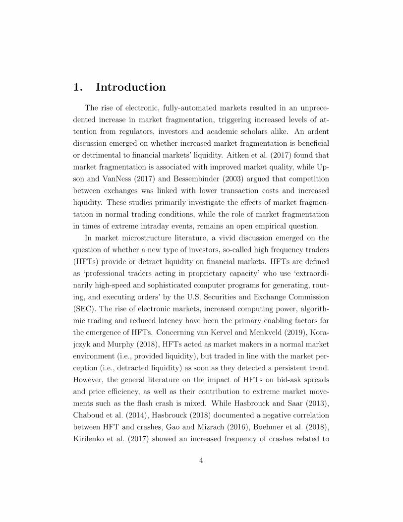
We analyzed investment returns around stock price crashes. Figure 1
shows an example of such a stock price crash for LBrands on February 23,
2017. The daily return calculated based on open and close price was −3.1%
on this day. However, the development of intraday prices exhibited high
volatility, i.e., prices took to reach new market equilibrium. Specifically, by
11:05 AM, LBrands was trading −5% lower than its open price, exhibiting
a steep declining pattern, followed by a period of recovery lasting up until
12:05, at which time LBrands was reporting −2% return for the day.
Hasbrouck and Saar (2013),Chordia et al. (2008) found that HFTs in-
crease liquidity in such extreme situations, being associated with greater
market efficiency (Carrion, 2013; Brogaard et al., 2014; Chaboud et al., 2014).
Moreover, Shkilko and Sokolov (2020) associate reduced HFT activity with
lower adverse selection and lower trading costs.
Thus, we state the hypothesis that during a price shock, market pric-
ing is inefficient only for a very short period due to overreactions. This
situation provides the opportunity to exploit the advantages of low-latency
5

data transfer and increased computational power to trade against the wind,
provide short-term liquidity, and gain returns from short-term stock price
reversals.
09:30 16:00
48
49
50
51
Time
Sto
ckpri
ce
Fig. 1. Intraday price development of LBrands on February 23, 2017.
On the topic of return reversals, a large body of literature addressed the
risk-bearing capacity of intermediaries (Kirilenko et al., 2017; Nagel, 2012;
Hameed and Mian, 2015). Nagel (2012), So and Wang (2014) showed that
providing liquidity during reversals is profitable. Furthermore, Handa and
Schwarz (1993) show that placing a network of buy and sell limit order as
part of a trading strategy is profitable. HFTs can react marginally faster to
market signals, and thus conduct so-called latency arbitrage and stale quote
sniping (Foucault et al., 2003; Menkveld and Zoican, 2017; Budish et al.,
2015). Brogaard et al. (2017), Brogaard et al. (2018) studied HFTs during a
short-sale ban and around extreme price movements. Empirical results (see
Hasbrouck and Sofianos, 1993; Madhavan and Smidt, 1993) highlighted that
intraday mean-reversion in inventories, and relatively high trading volume are
noticeable characteristics of intermediation, which are categorized as high-
frequency traders or high-frequency market makers (Biais et al., 2015; Ait-
6

Sahalia and Saglam, 2017; Jovanovic and Menkveld, 2016). Concerning the
finding of Brogaard et al. (2018), HFTs speed up the reversal process after
extreme price movements.
Fig. 2. This figure shows the average return profile across our set of 15,242identified extreme return intervals. It shows the minute returns during thefive individual minutes before and after extreme interval. All returns areexpressed in basis points.
Our study investigates the effect of market fragmentation and intraday
return patterns around extreme price movements. We analyze a sample of
intraday quote and trade data of the Nasdaq100 constituents for the period
from January 2014 to January 2019. We divide each trading day into 390
one-minute intervals and clustered intervals according to their returns in the
crash and non-crash intervals. Crash intervals exhibit characteristics (such as
return and trading activity) significantly different from non-crash intervals.
7

The one-minute return of a crash interval was 72 basis points lower than the
return of a non-crash interval (see Figure 2). Multivariate analyses show the
existence of an after-crash reversal, which is about 27% of the crash return,
while the reversal has the highest proportion of the crash return for firms
with high-liquid stocks and high firm size.
Figure 3 portrays an example of how the algorithmic crash identification
approach would flag and label the minute intervals based on an extreme event
occurring around t, whereby t − 1, t and t + 1 represent the cutoff points
delimiting fixed minuted intervals. The interval starting at t− 1 and ending
at t would be flagged as a crash interval, while consecutively the interval
beginning at t and ending at t+ 1 constitutes the follow-up reversal interval.
Consequently, it is important to note, that the algorithmic approach does
not take the minimum of a minute interval in calculating the returns, or
the crash return respectively, but rather relies on chronological delimiters
which are ex-ante defined to be fixed. While this does indeed potentially
cause understatements of crash and reversal returns, this approach ensures
the robustness and systematic nature of the identification algorithm.
t-1 t t+1
98
98.5
99
99.5
100
Fig. 3. Generic example of crash interval.
In an event study, whereby 45 Nasdaq100 constituents experienced a con-
8

comitant extreme negative price movements, we investigate differences in
trade and volume patterns between stocks with different degrees of market
fragmentation. On December 1st, 2017, between 11:14 AM and 11:15 AM the
market experienced an external shock, reacting to a news release reporting
that Michael Flynn pleaded guilty to lying to federal agents in the context
of President Trump’s Russian election interference investigation. By using
a difference-in-differences approach we find no evidence on discrepancies or
deviations in trade, volume and return patterns between stocks with an in-
creased volume split across individual exchanges and stocks whose trading
volume is concentrated on one single exchange. These results provide evi-
dence that market fragmentation does negatively affect the aforementioned
reversal process.
To the best of our knowledge, our study is the first one looking into the
role played by market fragmentation around extreme price movements. On
the topic of short term return reversals and HFT activity, one related paper is
Brogaard et al. (2018), which investigated the role of HFTs around extreme
stock price movements, in particular by analyzing quote data. In contrast,
our study examines the return structure around extreme return intervals by
relying on realized trade prices to capture real investment returns.
Using recent advances and increasing affordability in cloud computing
services the analysis included in this paper covers all the constituents in the
Nasdaq100 over the period from January 2014 to January 2019, in contrast
to the (post-)financial crisis period of 2008 and 2009 covered in Brogaard
et al. (2018). Additionally, we focused on downward price movements and
characterized the stock price development in an eleven-minute time window
around the crash minute. Moreover, we extend the results presented in Upson
and VanNess (2017) and Bessembinder (2003), who document a positive
effect of volume fragmentation on general market conditions.
The remainder of the paper proceeds as follows. In Section 2, we discuss
the data employed in this paper. In Section 3, we present our empirical
9

methodology and results. In Section 4, we conclude.
2. Data
We employed intraday trading data from the NYSE Daily Trade and
Quote (DTAQ) database available over the WRDS Cloud platform. Specif-
ically, we sourced data from the Daily TAQ files from where we retrieved
millisecond-level data from January 1st, 2014, microsecond level data start-
ing from July 27th, 2015, and nanosecond level data starting from October
24th, 2016. The data covers trade, quote, and national best bid and offer
(NBBO) data for a basket of the 100 stocks comprising the Nasdaq100. Our
observation period ranges from January 2014 to January 2019, yielding a
sample of 1,564,388,227 analyzed trades in total.
We restricted our data to trades and quotes posted within the regular
trading hours of the NYSE (9:30 a.m to 4:00 p.m.). Concerning the handling
of withdrawn quotes and quotes with abnormal conditions, we followed the
methodology outlined in Holden and Jacobsen (2014). Namely, we considered
crossed quotes (quotes where the bid price is higher than the ask price) if they
arose because the ask price was zero while the bid price was non-zero. We
excluded quotes with abnormal quote and trade conditions, such as situations
where trading has been halted. Further, we focused on trades of common
stocks in our sample. In this respect, we dropped any observation for which
the quote and trade conditions are listed as A, B, H, K, L, O, R, V, W, and
Z∗. We also excluded data points where the bid price is greater than the ask
price, if listed by the same exchange, or for which either price or quantity
was equal to zero. In line with Chordia et al. (2001), we also dropped any
data points where the quoted spread was higher than 5 USD.
We corrected the original NBBO daily file considering data from all of the
available exchanges following Holden and Jacobsen (2014). Subsequently, we
∗ Table 8 in the Appendix defines all abnormal trade and quote conditions.
10
matched trades with corresponding NBBO quotes at the microsecond level.
Based on this matched data set, we classified trades as buyer- or seller-
initiated trades in line with the classification method proposed by Lee and
Ready (1991).
3. Methodology and Results
A. Crash Intervals and Summary Statistics
To investigate the reversal returns after stock price crashes, we split each
trading day within the matched trade and NBBO quote data into fixed equal
one-minute time intervals. Hence, splitting a typical trading day resulted
in 390 individual one-minute intervals. One minute intervals may appear
very long compared to the time HFT algorithms require in order to re-
evaluate a trading strategy. While Brogaard et al. (2018) considered 10-
second-intervals, van Kervel and Menkveld (2019) 30-minutes update time
stamps. In particular, Brogaard et al. (2018) showed that prices continued
to move in the direction of the largest return for several seconds after the
first indication for an extreme price movement. In this respect, we decided
to use one-minute intervals. In unreported tests, we varied the time horizon
from 30 seconds to five minutes. The results stayed qualitatively similar.
For each interval, we then calculated the actual realized interval return
based on the recorded trades, the standard deviation of the realized returns
based on the within-interval realized trades, the minimum and the maximum
realized return within each interval. Additionally, we determined the average
quoted spread, the total traded share volume, and the net volume of shares
bought or sold within each one-minute interval.
Moreover, we relied on the literature on stock price crashes to identify ex-
treme price changes across the one-minute intervals. Therefore, we assigned
the strategy of Brogaard et al. (2018), Hutton et al. (2009) and defined a
one-minute interval as a crash interval if the actual return is an event oc-
11
curring once in a thousand observations, i.e., the 0.1%-quantile. Equation 1
shows the identification rule for crash interval variable Cm,ki,t :
Cm,ki,t =
1 ri,t ≤ µm,ki,t + Φ−1(0.001) · σm,k
i,t
0 ri,t > µm,ki,t + Φ−1(0.001) · σm,k
i,t
, (1)
where ri,t is the actual return of the respective one-minute interval t of firm
i, µm,ki,t is the expected return for firm i in one-minute interval t, σm,k
i,t is the
standard deviation of the expected return for firm i in one-minute interval t,
and Φ−1(0.001) = −3.09 represents the critical value for the 0.1%-quantile of
the standard normal distribution with mean zero and standard deviation one.
We specified µm,ki,t and σm,k
i,t according to two different conceptual procedures
(m = {1, 2}) to identify extreme downward price movements. k refers to the
number of historical observations that are used in either procedure.
The first procedure (m = 1) considered consecutive k previous one-minute
intervals to estimate the expected interval return and its standard deviation.
We used a varying number of observations k in Equation 1 corresponding
to 5, 15, and 60 previous one-minute intervals, as well as 390 one-minute
intervals for one day, 1950 one-minute intervals for one week, 40,950 one-
minute intervals for one month, and 122,850 one-minute intervals for one
quarter-time spans.
Our second procedure (m = 2) used matched time intervals, as opposed
to consecutive time intervals. We defined a matched time interval as the
interval corresponding to the identical time interval, albeit in a prior trading
day. For instance, yesterday‘s first trading minute (9:30:00-9:31:00) served
as a matched interval for today‘s first trading minute. The second procedure
addressed the significantly different intraday return pattern of large returns
in the early morning, which leveled off during the day. Therefore, we as-
sessed whether an interval classifies as a stock price crash by determining the
crash variable of Equation 1 based on 5, 21, 63, and 252 matched intervals,
corresponding to a week, month, quarter, and one year time spans.
12

Finally, we defined a crash dummy variable Ci,t for each one-minute in-
terval t of a specific firm i. The crash dummy equals one if all of the above-
mentioned identification methods flag the interval as a crash interval and
zero otherwise:
Ci,t =
1 Cm,ki,t = 1 ∀m, k
0 otherwise, (2)
In total, we identified 15,242 one-minute intervals, which we labeled as
crash intervals, while 46,773,469 one-minute intervals show no extreme down-
ward movements (see Table 1). Panel A of Table 1 provides pooled raw
descriptive statistics of our data set, contrasting the characteristics of non-
crash and crash intervals. The first set of columns reports values for the
non-crash intervals. The mean bid-ask spread in a non-crash one-minute in-
terval was 5.72 basis points (bp). This number almost tripled in crash inter-
vals (14.67bp). In particular, the standard deviation of the bid-ask spreads
among the one-minute intervals is substantially higher for crash intervals
than for non-crash intervals (43.52bp vs 13.24bp). While the return of non-
crash one-minute intervals was 0.02bp on average, crash intervals observed
an average return of −72.03bp. The standard deviation of the one-minute re-
turns observed for crash intervals was ten times larger than the one observed
for non-crash intervals. In a 10th percentile one-minute crash interval, the
return was −145.17bp compared to −8.18bp in a non-crash interval.
Moreover, we calculated the minimum and maximum returns between two
subsequent trades in each one-minute interval. Non-crash intervals exhibited
on average −4.9bp for the minimum and 4.93bp for the maximum. The
range from the 10th percentile of the minimum return (−9.6bp) and the
90th percentile of the maximum return (9.63bp) was rather narrow. The
respective quantities in crash intervals showed a substantially higher variation
in trading returns. While the 10th percentile of the minimum return equaled
a return lower than −1%, we also observed high positive returns of 50bp
13

(90th percentile of the maximum return).
We constructed a momentum indicator that counts the number of succes-
sive intervals during which negative (positive) realized returns were observed.
I.e., if we obtained negative returns in Intervals t − 3, t − 2, and t − 1, the
value of the momentum variable for Interval t is −3. Symmetrically, if the
series of interval returns were positive, the momentum indicator takes the
value of +3. Alternatively, if returns in intervals t−3 and t−1 were negative
but positive in the Interval t− 2, the momentum indicator for Interval t is 0
as a change in sign has been recorded.
The average momentum of non-crash intervals is 0.28, the 10th percentile
of the momentum was −1, and the 90th percentile of the momentum was
2. These values indicate a market structure with mostly alternating one-
minute interval returns with only 10% observations with at least a series
of two subsequent negative one-minute interval returns and another 10%
observations with at least a series of three subsequent positive one-minute
interval returns. Crash intervals, however, occurred on average after two
prior one-minute intervals with negative returns. Only 10% of the crash
intervals were preceded by a series of at least three one-minute intervals with
a negative return.
A fundamental distinction between non-crash and crash intervals was the
trading activity in the respective one-minute interval in terms of trading
volume and number of trades. While the number of actual trades recorded
within an interval increased more than threefold vs a non-crash interval, the
average trading volume in the crash intervals was approximately 7.5 times
higher. On average, 13,500 shares were traded in a non-crash one-minute
interval, while 101,180 shares were traded in a crash one-minute interval. The
increased volume was due to a substantially higher number of trades in the
respective intervals (215 vs 717). The negative average of the LRQty variable
(the LRQty is the number of buyer-initiated trades minus the number of
seller-initiated trades) indicated that during crash intervals, a substantially
14

Tab
le1:
This
table
rep
orts
onp
ool
edra
wan
dst
andar
diz
eddes
crip
tive
stat
isti
csfo
rcr
ash
and
non
-cra
shm
inute
inte
rval
s.O
ur
sam
ple
consi
sts
ofal
ltr
ades
and
quot
esfo
rth
eco
nst
ituen
tsof
the
Nas
daq
100
thro
ugh
out
anob
serv
atio
np
erio
dra
ngi
ng
from
Jan
uar
y20
14to
Jan
uar
y20
19ag
greg
ated
into
one-
min
ute
inte
rval
s.T
he
unit
ofth
ere
por
ted
spre
adan
dre
turn
quan
titi
esis
bas
isp
oints
.
Non
-Cra
shIn
terv
als
(N=
46,7
73,4
69)
Cra
shIn
terv
als
(N=
15,2
42)
Mea
nS
D10
th%
ile
Med
ian
90th
%il
eM
ean
SD
10th
%il
eM
edia
n90
th%
ile
Pan
elA
:R
awqu
anti
ties
Bid
Ask
5.72
13.2
41.
553.
3010
.59
14.6
743
.52
1.94
5.55
26.9
6R
et0.
028.
94−
8.18
0.00
8.17−
72.0
380
.16−
145.
17−
46.3
9−
23.6
0M
inR
et−
4.90
9.28
−9.
60−
3.23
−1.
27−
44.9
086
.14−
106.
77−
17.6
8−
4.65
Max
Ret
4.93
9.37
1.28
3.24
9.63
22.6
567
.69
2.04
9.04
52.8
0S
D1.
842.
700.
551.
203.
568.
9222
.50
0.98
2.93
19.2
2M
om0.
261.
67−
1.00
0.00
2.00
−0.
881.
44−
3.00
0.00
0.00
Vol
13.5
054
.63
0.51
3.99
29.3
510
1.18
292.
142.
3023
.80
235.
63N
rTrd
215.
4638
1.79
20.0
095
.00
504.
0071
7.98
1,29
7.18
58.1
031
2.50
1,66
0.00
LR
Qty
−0.
6139
.94
−3.
95−
19.0
03.
68−
34.1
616
8.01
−71
.08
−6.
220.
90
Pan
elB
:S
tan
dard
ized
quan
titi
esB
idA
sk−
5.84
E−
40.
99−
0.64
−0.
140.
701.
828.
38−
0.40
0.22
3.71
Ret
2.66
E−
30.
97−
0.93−
4.54
E−
40.
93−
8.16
9.39
−15
.98
−5.
16−
3.04
Min
Ret
1.52
E−
30.
98−
0.46
0.14
0.41
−4.
6610
.24−
11.6
6−
1.39
−0.
03M
axR
et−
6.56
E−
40.
99−
0.41
−0.
140.
462.
017.
87−
0.28
0.44
5.55
SD−
9.96
E−
40.
99−
0.50
−0.
160.
563.
089.
06−
0.25
0.51
7.80
Mom
2.26
E−
41.
00−
0.81
−0.
131.
11−
0.70
0.88
−1.
93−
0.24
−0.
07V
ol−
8.13
E−
40.
99−
0.40
−0.
190.
472.
505.
39−
0.22
0.87
6.38
NrT
rd−
6.85
E−
41.
00−
0.76
−0.
271.
032.
103.
40−
0.45
1.21
5.41
LR
Qty
4.27
E−
41.
00−
0.26
4.27
E−
40.
25−
1.31
4.50
−3.
51−
0.50
0.08
15

higher number of trades were seller-initiated trades compared to non-crash
intervals.
Panel B of Table 1 provides the same statistics after a z-transformation
of the interval statistics. We present these quantities to capture the effect of
the difference in absolute values of single firms. For instance, trading volume
significantly varies across firms. Even after controlling for firm-specific in-
fluences, the summary statistics display a similar relationship between non-
crash and crash intervals. Since the average values of all variables in the
non-crash sample were almost zero, the average z-scores of the crash sample
indicated the significance level of the crash interval variables different from
zero (alternative hypothesis). Except for the momentum and the LRQty
variables, all other variables were significantly different from zero, and thus
from the ones of the non-crash sample.
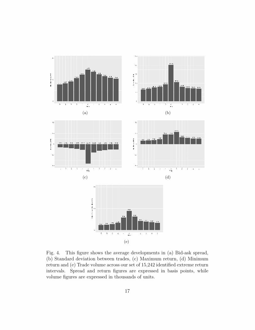
We continued focusing on the crash interval. We investigated the consec-
utive one-minute intervals five minutes before and after the crash interval to
understand the development of the variables around such an extreme event.
Therefore, we structured the bid-ask spread, the return standard deviation
(between single trades), the average minimum return, the average maximum
return, and the trade volume in event-time and aggregated each variable
across the cross-section. Figure 4 exhibits the development of these vari-
ables. We observed a gradual increase in the quoted bid-ask spread, peaking
in the crash interval followed by a moderate, gradual recovery in the follow-
up minute intervals (Subfigure (a)). The recorded trading volume (Subfigure
(b)) exhibited a spike pattern, with minimal increases in the five minutes
running up to the crash, followed by a more than twofold increase in the
actual crash interval. This pattern suggests that traders with a fast reaction
could be behind such an increase in trading activity.
Turning to the metrics calculated based on the individual within-interval
trades, we observed a similar pattern such as the one of the quoted spread
for the standard deviation of realized returns (Subfigure (e)). The average
16
(a) (b)
(c) (d)
(e)
Fig. 4. This figure shows the average developments in (a) Bid-ask spread,(b) Standard deviation between trades, (c) Maximum return, (d) Minimumreturn and (e) Trade volume across our set of 15,242 identified extreme returnintervals. Spread and return figures are expressed in basis points, whilevolume figures are expressed in thousands of units.
17

minimum return between two trades showed downward spikes, which were
more than three times smaller during the crash minute than in the minutes
before the event (Subfigure (c)). Conversely, the average maximum return
increased considerably, effectively doubling in t−1 and staying at this level in
t, it reached its peak only in t+1, providing preliminary evidence supporting
the idea of a trading strategy aimed at capitalizing on a potential overreaction
taking place in t and a possible reversal in t+ 1.
B. Structure of One-Minute Interval Returns
We began with an analysis of the one-minute interval returns. Therefore,
we ran OLS regression models with firm and year fixed-effects, and clustered
standard errors on firm-level (Equation 3):
Reti,t = β0 + Θ · Controlsi + αi + ut + εit (3)
where Θ is the vector of coefficients of the independent variables, αi is
the firm fixed effect, ut is the time fixed effect, and εit is the error term. We
estimated nine different model specifications. The dependent variable was
the log return (in basis points) of each of our 46 million one-minute interval
observations. We organized the data according to the event time and used
each one-minute interval as the interval under consideration once, i.e., its
index is t. We explained the variation of these one-minute interval returns of
index t by a set of control variables including crash dummy variable, the log
returns observed in the five one-minute intervals before and after the analyzed
minute interval t, the momentum observed as of t−1, as well as the standard
deviation of within interval returns, the bid-ask spread, and trading volume
recorded across the previous individual five one-minute intervals. Moreover,
we include interaction variables between the five lagged and lead returns and
the crash dummy to investigate the specific return structure before and after
crash intervals. The nine model specifications distinguished by the subset
18

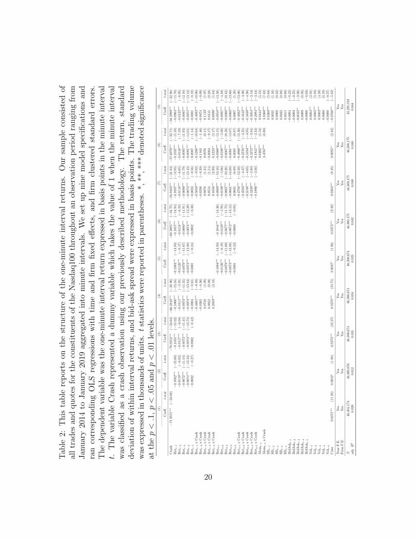
of control variables we included in the estimation. Model specification (9)
contains the entire list of control variables.
In the first model specification, we explained the variation of the log
returns of the one-minute intervals with the crash dummy variable (see Ta-
ble 2). According to the estimation, the coefficient of the crash dummy in
Model (1) showed that intervals flagged as crash intervals exhibited on aver-
age a return which is about 72bp lower when compared to the average returns
of non-crash intervals. The coefficient was strongly significant different from
zero. We augmented this model specification by lagged and lead returns and
their interactions with the crash dummy in model specifications (2) – (7).
Although the coefficient of the dummy variable slightly reduced in magni-
tude, it remained statistically significantly different from zero at a p < 0.01
level.
In line with extant literature, we observed and confirmed a negative cor-
relation structure between the returns experienced in the pre- and post-crash
intervals. This negative correlation structure remains constant throughout
model specifications (2) to (9) with statistically significant and negative co-
efficients displayed for the four interval returns before the Interval t. The
strongest effect was observed for Interval t−1, where the negative coefficient
for Rett−1 suggests the occurrence of a reversal in t, quantifying to roughly
10% of the return recorded in Interval t−1. We observed a similar correlation
pattern when looking at returns recorded in the four one-minute intervals af-
ter t in model specifications (5) to (9). The negative coefficient for Rett+1
is symmetrical in magnitude and sign to the coefficient reported for Rett−1
pointing to the existence of a return reversal, which is strongest in t+1. This
pattern supported an alternating return development in which the current
return shows a 10% reversal of the return of the last one-minute interval.
We further noticed that the occurrence of a crash in t has a statistically
significant and amplifying effect on the observed return structure. For crash
intervals, the reversal pattern was intensified since the coefficient of the in-
19
Tab
le2:
This
table
rep
orts
onth
est
ruct
ure
ofth
eon
e-m
inute
inte
rval
retu
rns.
Our
sam
ple
consi
sted
ofal
ltr
ades
and
quot
esfo
rth
eco
nst
ituen
tsof
the
Nas
daq
100
thro
ugh
out
anob
serv
atio
np
erio
dra
ngi
ng
from
Jan
uar
y20
14to
Jan
uar
y20
19ag
greg
ated
into
min
ute
inte
rval
s.W
ese
tup
nin
em
odel
spec
ifica
tion
san
dra
nco
rres
pon
din
gO
LS
regr
essi
ons
wit
hti
me
and
firm
fixed
effec
ts,
and
firm
clust
ered
stan
dar
der
rors
.T
he
dep
enden
tva
riab
lew
asth
eon
e-m
inute
inte
rval
retu
rnex
pre
ssed
inbas
isp
oints
inth
em
inute
inte
rval
t.T
he
vari
able
Cra
shre
pre
sente
da
dum
my
vari
able
whic
hta
kes
the
valu
eof
1w
hen
the
min
ute
inte
rval
was
clas
sified
asa
cras
hob
serv
atio
nusi
ng
our
pre
vio
usl
ydes
crib
edm
ethodol
ogy.
The
retu
rn,
stan
dar
ddev
iati
onof
wit
hin
inte
rval
retu
rns,
and
bid
-ask
spre
adw
ere
expre
ssed
inbas
isp
oints
.T
he
trad
ing
volu
me
was
expre
ssed
inth
ousa
nds
ofunit
s.t
stat
isti
csw
ere
rep
orte
din
par
enth
eses
.*,
**,**
*den
oted
sign
ifica
nce
atth
ep<.1
,p<.0
5an
dp<.0
1le
vels
.(1
)(2
)(3
)(4
)(5
)(6
)(7
)(8
)(9
)
Coeff
.t-
stat
Coeff
.t-
stat
Coeff
.t-
stat
Coeff
.t-
stat
Coeff
.t-
stat
Coeff
.t-
stat
Coeff
.t-
stat
Coeff
.t-
stat
Coeff
.t-
stat
Cra
sh−
71.9
571∗∗∗
(−33
.08)
−70
.925
2∗∗∗
(−34
.64)−
66.2
842∗∗∗
(−38
.96)
−69
.389
5∗∗∗
(−34
.75)−
56.9
403∗∗∗
(−31
.83)−
57.6
979∗∗∗
(−32
.71)−
58.2
999∗∗∗
(−32
.90)
Ret
t−1
−0.
1082∗∗∗
(−15
.00)
−0.
1055∗∗∗
(−15
.02)
−0.
1006∗∗∗
(−15
.05)−
0.10
84∗∗∗
(−14
.93)
−0.
1057∗∗∗
(−14
.94)
−0.
1007∗∗∗
(−14
.95)
−0.
1037∗∗∗
(−15
.50)
−0.
0964∗∗∗
(−15
.70)
Ret
t−2
−0.
0119∗∗∗
(−6.
02)−
0.01
17∗∗∗
(−6.
04)−
0.01
11∗∗∗
(−5.
91)−
0.01
26∗∗∗
(−6.
17)−
0.01
24∗∗∗
(−6.
19)−
0.01
18∗∗∗
(−6.
05)−
0.01
48∗∗∗
(−7.
19)−
0.01
23∗∗∗
(−6.
95)
Ret
t−3
−0.
0072∗∗∗
(−11
.14)
−0.
0073∗∗∗
(−11
.41)
−0.
0074∗∗∗
(−11
.35)−
0.00
79∗∗∗
(−11
.67)
−0.
0080∗∗∗
(−11
.91)
−0.
0080∗∗∗
(−11
.79)
−0.
0095∗∗∗
(−11
.93)
−0.
0085∗∗∗
(−12
.10)
Ret
t−4
−0.
0074∗∗∗
(−13
.34)
−0.
0074∗∗∗
(−13
.75)
−0.
0074∗∗∗
(−13
.84)−
0.00
73∗∗∗
(−12
.88)
−0.
0074∗∗∗
(−13
.29)
−0.
0074∗∗∗
(−13
.43)
−0.
0081∗∗∗
(−14
.01)
−0.
0075∗∗∗
(−13
.12)
Ret
t−5
−0.
0002
(−0.
27)−
0.00
02(−
0.42
)−
0.00
04(−
0.61
)−
0.00
01(−
0.24
)−
0.00
02(−
0.38
)−
0.00
03(−
0.56
)−
0.00
07(−
1.14
)−
0.00
01(−
0.18
)R
ett−
1x
Cra
sh−
0.46
81∗∗∗
(−8.
40)
−0.
5050∗∗∗
(−9.
92)−
0.52
80∗∗∗
(−10
.64)
−0.
4883∗∗∗
(−10
.06)
Ret
t−2
xC
rash
−0.
0265
(−0.
36)
−0.
0290
(−0.
39)−
0.11
63(−
1.46
)−
0.00
74(−
0.09
)R
ett−
3x
Cra
sh0.
0758
(1.0
9)0.
0876
(1.2
4)0.
0076
(0.1
1)0.
1133∗
(1.9
7)R
ett−
4x
Cra
sh0.
0052
(0.0
8)0.
0554
(1.1
4)−
0.00
84(−
0.17
)0.
0141
(0.2
8)R
ett−
5x
Cra
sh0.
2059∗∗∗
(3.1
8)0.
1656∗∗∗
(2.8
9)0.
1223∗∗
(2.1
7)0.
0998∗
(1.8
4)R
ett+
1−
0.10
84∗∗∗
(−14
.93)
−0.
1044∗∗∗
(−14
.36)
−0.
0989∗∗∗
(−13
.16)
−0.
0989∗∗∗
(−13
.15)
−0.
0918∗∗∗
(−13
.38)
Ret
t+2
−0.
0126∗∗∗
(−6.
18)−
0.01
20∗∗∗
(−5.
95)−
0.01
00∗∗∗
(−5.
06)−
0.01
00∗∗∗
(−5.
06)−
0.00
81∗∗∗
(−4.
48)
Ret
t+3
−0.
0079∗∗∗
(−11
.69)
−0.
0077∗∗∗
(−11
.75)
−0.
0067∗∗∗
(−10
.26)
−0.
0067∗∗∗
(−10
.26)
−0.
0060∗∗∗
(−10
.42)
Ret
t+4
−0.
0073∗∗∗
(−12
.88)
−0.
0072∗∗∗
(−13
.12)
−0.
0061∗∗∗
(−14
.08)
−0.
0061∗∗∗
(−14
.07)
−0.
0060∗∗∗
(−13
.60)
Ret
t+5
−0.
0001
(−0.
23)−
0.00
00(−
0.05
)0.
0005
(0.8
9)0.
0005
(0.8
7)0.
0007
(1.2
0)R
ett+
1x
Cra
sh−
0.47
94∗∗∗
(−13
.38)
−0.
4806∗∗∗
(−13
.46)
−0.
4882∗∗∗
(−13
.06)
Ret
t+2
xC
rash
−0.
3593∗∗∗
(−4.
37)−
0.35
76∗∗∗
(−4.
35)−
0.34
42∗∗∗
(−4.
08)
Ret
t+3
xC
rash
−0.
3188∗∗∗
(−4.
05)−
0.31
94∗∗∗
(−4.
05)−
0.34
38∗∗∗
(−4.
30)
Ret
t+4
xC
rash
−0.
3339∗∗∗
(−3.
80)−
0.33
72∗∗∗
(−3.
84)−
0.30
54∗∗∗
(−3.
54)
Ret
t+5
xC
rash
−0.
1896∗∗∗
(−3.
56)−
0.18
45∗∗∗
(−3.
43)−
0.20
94∗∗∗
(−3.
44)
Mom
t−1
0.04
62∗∗∗
(5.5
4)0.
0444∗∗∗
(5.5
5)M
omt−
1x
Cra
sh3.
4767∗∗∗
(8.8
0)2.
8368∗∗∗
(7.4
2)SD
t−1
0.03
68∗∗∗
(5.6
8)SD
t−2
0.00
31(1
.16)
SD
t−3
0.00
08(0
.32)
SD
t−4
0.00
22(0
.89)
SD
t−5
0.00
15(0
.68)
Bid
Ask
t−1
−0.
0004
(−0.
22)
Bid
Ask
t−2
−0.
0003
(−0.
25)
Bid
Ask
t−3
−0.
0023∗∗
(−2.
00)
Bid
Ask
t−4
0.00
09(0
.95)
Bid
Ask
t−5
−0.
0000
(−0.
03)
Vol
t−1
0.00
04∗∗∗
(2.9
1)V
olt−
20.
0005∗∗∗
(5.9
4)V
olt−
30.
0003∗∗∗
(4.3
9)V
olt−
40.
0000
(0.1
9)V
olt−
5−
0.00
00(−
0.37
)C
ons
0.02
71∗∗∗
(11.
26)
0.00
42∗
(1.8
6)0.
0273∗∗∗
(10.
37)
0.02
70∗∗∗
(10.
75)
0.00
47∗
(1.8
6)0.
0273∗∗∗
(9.4
8)0.
0263∗∗∗
(9.4
5)0.
0095∗∗
(2.4
4)−
0.07
66∗∗∗
(−5.
82)
Yea
rF
.E.
Yes
Yes
Yes
Yes
Yes
Yes
Yes
Yes
Yes
Fir
mF
.E.
Yes
Yes
Yes
Yes
Yes
Yes
Yes
Yes
Yes
N46
,301
,174
46,3
00,6
7646
,300
,674
46,3
00,6
7446
,300
,674
46,3
00,1
7546
,300
,175
46,3
00,1
7543
,291
,019
adj.R
20.
020
0.01
20.
031
0.03
40.
023
0.04
20.
048
0.04
80.
044
20

teraction term of Rett−1 and the crash dummy was about −0.5. Specifically,
a one basis point increase in Rett−1 is associated, on average, with a crash re-
turn which was 0.5bp more negative than the return in a non-crash interval.
I.e., if the one-minute interval t was a crash interval, the log return in this
interval was 0.5 · Rett−1 smaller than for a non-crash interval. Additionally,
we observed the return reversal in the one-minute interval after the crash.
This effect is symmetrical when looking at the observed coefficients reported
for the interaction terms between the crash dummy and the lead five returns
reported in model specifications (7), (8), and (9). The log return of a firm
experiencing a stock price crash in t showed a stock price reversal in the
first minute after the crash which is 48% ·Rett higher as the reversal after a
non-crash interval.
Referring to Model (8), we observed a positive, statistically significant
impact of the momentum indicator on the return recorded in Interval t.
Given the average momentum of 0.2 as computed for non-crash intervals,
momentum had a minor impact on the magnitude of the return recorded in
t when no crash was recorded. This effect was substantially amplified when
looking at crash intervals. Specifically, any unit decrease in momentum was
associated with a crash return which was, on average, roughly 3.5bp lower.
The standard deviation of within interval returns and the observed bid-
ask spread had a weak and immaterial association with the return in Interval
t. The reported coefficients in Model (9) were statistically insignificant apart
from the coefficient for the bid-ask spread at t− 3, which nevertheless could
be regarded as immaterial given the average size of quoted bid-ask spread.
Similarly, while the coefficients of the lagged trading volume were strongly
statistically significant, they showed no material association with the return
at t.
21

C. Reversal Return After Crash Intervals
We continued our analysis on the subset of crash one-minute intervals to
study the return reversals after a crash. Therefore, we explained the variation
of the log returns of the one-minute crash interval one minute after the crash
by the crash interval return and further control variables:
Reti,t+1 = β0 + β1 ·Rett + Γ · Controlsi + αi + ut + εit (4)
where Γ is the vector of coefficients of the independent variables, αi is the
firm fixed effect, ut is the time fixed effect, and εit is the error term.
The negative and statistically significant coefficients for Rett across all
four model specifications showed that indeed, a reversal was present (see
Table 3). The magnitude of this reversal, one minute after the crash interval,
was about 27% of the size of the log return during the crash interval (see
model specification (1)). Furthermore, Model (2) showed that the return
of the interval before the crash interval was also associated with the return
in the reversal Interval t + 1. Namely, a positive return of one basis point
recorded in the Interval t − 1 is associated with a 0.2 basis point reduction
of the reversal in t + 1. Model (3) documented a positive and statistically
significant association between the return in the reversal interval and the
momentum variable before the crash. Specifically, a positive momentum up
to the crash interval is linked to a stronger reversal. Each unit increase in
the momentum variable was linked to a 1.3 basis point increase in the return
observed in the recovery interval.
D. Firm Characteristics and the Magnitude of the Crash Re-
versal Return
Given the strong statistical evidence documenting the occurrence of a
reversal in Interval t + 1, we further analyzed the influence of firm charac-
teristics on the size of the reversal. Accordingly, we split our sample of firms
22

Table 3: This table reports the estimates of the OLS regression model withtime and firm fixed effects, and firm clustered standard errors explainingthe variation in the one-minute interval return in t + 1 as a function of aset of independent variables. We estimated four model specifications. Thereturn, standard deviation of within interval returns, and bid-ask spread areexpressed in basis points. The trading volume is expressed in thousands ofunits. t statistics are reported in parentheses. *, **, *** denote significanceat the p < .1, p < .05 and p < .01 levels.
Dependent variable: post-crash one-minute interval returns (RetT+1)
(1) (2) (3) (4)
Coeff. t-stat Coeff. t-stat Coeff. t-stat Coeff. t-stat
Rett −0.2682∗∗∗ (−8.32) −0.3115∗∗∗ (−9.03) −0.3144∗∗∗ (−9.05) −0.3060∗∗∗ (−9.19)Rett−1 −0.2040∗∗∗ (−8.42) −0.2168∗∗∗ (−8.59) −0.2312∗∗∗ (−6.47)Rett−2 0.0128 (0.31) −0.0247 (−0.57) 0.0018 (0.04)Rett−3 0.0796∗∗ (2.10) 0.0464 (1.19) 0.0937∗∗ (2.59)Rett−4 0.1159∗∗ (2.25) 0.0898∗ (1.73) 0.0738 (1.47)Rett−5 0.0554 (1.33) 0.0383 (0.92) 0.0403 (0.77)Momt−1 1.4708∗∗∗ (5.64) 1.3008∗∗∗ (4.97)SDt−1 0.1028 (0.75)SDt−2 0.1756 (0.67)SDt−3 0.5654 (1.62)SDt−4 −0.0928 (−0.20)SDt−5 1.6303∗∗ (2.11)BidAskt−1 0.0395 (0.89)BidAskt−2 −0.0995 (−0.89)BidAskt−3 −0.0453∗ (−1.73)BidAskt−4 0.0173 (0.19)BidAskt−5 −0.3130 (−1.31)Volt−1 0.0050 (0.80)Volt−2 −0.0212∗∗∗ (−3.54)Volt−3 −0.0063∗ (−1.80)Volt−4 −0.0069 (−1.30)Volt−5 −0.0231∗∗∗ (−4.21)Cons −6.0925∗∗∗ (−2.72) −7.3186∗∗∗ (−3.21) −8.0047∗∗∗ (−3.42) −9.6215∗∗∗ (−4.14)
Year F.E. Yes Yes Yes YesFirm F.E. Yes Yes Yes Yes
N 15,104 15,102 15,102 14,135adj. R2 0.141 0.171 0.174 0.196
23

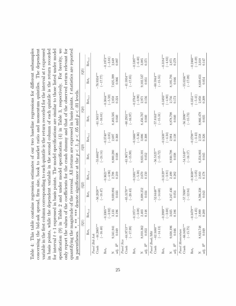
into quintiles, from smallest to largest, with respect to the observed bid-ask
spread, firm size, book to market ratio, and momentum. For each of these
sub-samples, we repeated the estimation of the model specification (9) of
Equation 3 and model specification (4) of Equation 4.
The results strengthened our previous findings, observing statistically sig-
nificant reversal coefficients across all sub-samples and all in line with our
previous narrative (see Table 4).† We observed that the firms with the largest
average bid-ask spread (Quintile 5 in Panel Bid-Ask), experienced the steep-
est crash, which was −76.93bp versus −44.2bp reported for the most liquid
firms in Quintile 1. Concurrently, the reversal after the crash was strongest
in Quintile 1, where we observed a rebound quantified to 33.05% of the re-
turn in the crash interval, as opposed to a recovery of only 19.73% of the
crash drop observed for the least liquid companies.
Conversely, we observed a similar pattern when splitting our sample ac-
cording to firm size measured by market capitalization. The largest firms
exhibited the smallest crash returns of −44.59bp, but the strongest reversal
of 53.97% in terms of the proportion of the magnitude of the crash return.
Moreover, under this specification, we also reported the best model fit with
an adjusted R2 of 0.371. Concerning the remaining two panels (book to mar-
ket ratio and momentum indicator), the results across the quintile groups are
not particularly distinctive.
†For the brevity of the reported results, Table 4 contained only the coefficients of thecrash dummy and the reversal coefficient for each panel-quintile combination, respectively.We quantified the magnitude of the average unexplained crash return at t and reported thecoefficient of the crash dummy variable of Equation 3 in the first column of each panel-quintile combination. The second column in each panel-quintile combination containedthe coefficient to quantify the reversal. Therefore, we reran the regression defined undermodel specification (4) in Equation 4. Additionally, we reported on model characteristics,i.e., the number of observations and the adjusted R2 of the respective model.
24
Tab
le4:
This
table
conta
ins
regr
essi
ones
tim
ates
ofou
rtw
obas
elin
ere
gres
sion
sfo
rdiff
eren
tsu
bsa
mple
sco
nce
rnin
gth
ebid
-ask
spre
ad,
firm
size
,b
ook
tom
arke
tra
tio
and
mom
entu
mquin
tile
s.T
he
dep
enden
tva
riab
lein
the
firs
tco
lum
nco
rres
pon
din
gto
each
quin
tile
isth
ere
turn
reco
rded
for
the
inte
rval
att
expre
ssed
inbas
isp
oints
,w
hile
the
dep
enden
tva
riab
lein
the
seco
nd
colu
mn
ofea
chquin
tile
isth
ere
turn
reco
rded
for
inte
rvalt+
1ex
pre
ssed
inbas
isp
oints
.T
he
model
spec
ifica
tion
sar
esi
milar
toth
ose
list
edunder
model
spec
ifica
tion
(9)
inT
able
2an
dunder
model
spec
ifica
tion
(4)
inT
able
3,re
spec
tive
ly.
For
bre
vit
y,w
eon
lyre
por
tth
eva
lues
ofth
eco
effici
ents
for
the
cras
hdum
my
and
that
ofth
eob
serv
edre
turn
rele
vant
for
quan
tify
ing
the
mag
nit
ude
ofth
ere
vers
al.
All
retu
rns
are
expre
ssed
inbas
isp
oints
.t
stat
isti
csar
ere
por
ted
inpar
enth
eses
.*,
**,
***
den
ote
sign
ifica
nce
atth
ep<.1
,p<.0
5an
dp<.0
1le
vels
.(Q
1)(Q
2)(Q
3)(Q
4)(Q
5)
Ret
tR
ett+
1R
ett
Ret
t+1
Ret
tR
ett+
1R
ett
Ret
t+1
Ret
tR
ett+
1
Pan
elB
id-A
skC
rash
−44
.200
5∗∗∗
−56
.202
8∗∗∗
−55
.688
2∗∗∗
−61
.501
5∗∗∗
−76
.933
4∗∗∗
(−16
.40)
(−18
.47)
(−24
.14)
(−16
.81)
(−17
.77)
Ret
t−
0.33
05∗∗∗
−0.
3621∗∗∗
−0.
3740∗∗∗
−0.
3044∗∗∗
−0.
1973∗∗∗
(−3.
92)
(−4.
96)
(−3.
85)
(−5.
59)
(−3.
81)
N9,
341,
941
3,13
39,
039,
894
2,79
88,
800,
280
2,69
78,
483,
505
2,85
87,
625,
399
2,64
9ad
j.R
20.
049
0.19
60.
033
0.21
90.
038
0.36
80.
040
0.22
40.
066
0.09
7
Pan
elS
ize
Cra
sh−
64.9
713∗∗∗
−65
.317
0∗∗∗
−61
.967
1∗∗∗
−60
.293
1∗∗∗
−41
.593
4∗∗∗
(−17
.99)
(−20
.43)
(−15
.99)
(−16
.97)
(−17
.85)
Ret
t−
0.19
71∗∗∗
−0.
2401∗∗∗
−0.
3466∗∗∗
−0.
2764∗∗∗
−0.
5397∗∗∗
(−3.
08)
(−5.
38)
(−5.
36)
(−3.
98)
(−6.
40)
N8,
010,
362
2,40
38,
698,
252
2,67
09,
023,
101
3,00
68,
456,
767
2,97
19,
102,
537
3,08
5ad
j.R
20.
053
0.14
80.
034
0.15
00.
052
0.30
80.
040
0.15
60.
051
0.37
1
Pan
elB
ook/
Mkt
Cra
sh−
62.3
480∗∗∗
−52
.644
8∗∗∗
−56
.512
5∗∗∗
−57
.816
3∗∗∗
−60
.594
4∗∗∗
(−14
.13)
(−14
.68)
(−15
.72)
(−15
.31)
(−15
.55)
Ret
t−
0.29
89∗∗∗
−0.
3129∗∗∗
−0.
2438∗∗∗
−0.
3493∗∗∗
−0.
3184∗∗∗
(−3.
68)
(−3.
81)
(−4.
34)
(−4.
80)
(−4.
83)
N9,
038,
196
3,02
58,
247,
436
2,49
98,
930,
798
2,98
48,
878,
798
2,75
68,
195,
791
2,87
1ad
j.R
20.
046
0.18
60.
054
0.28
20.
038
0.13
80.
040
0.17
30.
046
0.27
9
Pan
elM
omen
tum
Cra
sh−
66.8
491∗∗∗
−57
.769
0∗∗∗
−54
.514
9∗∗∗
−56
.289
0∗∗∗
−55
.024
6∗∗∗
(−15
.75)
(−12
.84)
(−16
.17)
(−15
.73)
(−17
.09)
Ret
t−
0.34
79∗∗∗
−0.
3038∗∗∗
−0.
2798∗∗∗
−0.
3351∗∗∗
−0.
2460∗∗∗
(−4.
45)
(−5.
05)
(−3.
43)
(−5.
41)
(−3.
49)
N8,
823,
748
2,89
98,
596,
338
2,81
08,
354,
803
2,55
88,
866,
479
2,85
08,
649,
651
3,01
8ad
j.R
20.
049
0.20
90.
043
0.17
80.
045
0.32
60.
035
0.20
90.
054
0.14
7
25

E. Market fragmentation and post-event trading
The increasing degree of market fragmentation observed throughout the
last two decades has attracted attention from scholars and regulators alike.
A large number of studies aimed at understanding the effects of market frag-
mentation have shed light on the effects that market fragmentation has on
general market conditions. In fact, Aitken et al. (2017) found that market
fragmentation is associated with improved market quality, while Upson and
VanNess (2017) and Bessembinder (2003) argued that competition between
exchanges was linked with lower transaction costs and increased liquidity.
However, the role of market fragmentation in a period of extreme returns
remains an open empirical question. This question is particularly important
for our setting, since distinct market conditions on different exchanges might
impact our results regarding actual achieved reversal returns.
To understand the impact of listing concentration on post-event return
reversals, we applied a quasi-natural experiment. We identified December
1st, 2017, as an event day, on which 45 Nasdaq100 constituents (see Table 9)
experienced an extreme negative price movement between 11:14 AM and
11:15 AM. The market reacted to a news release reporting that Michael Flynn
pleaded guilty to lying to federal agents in the context of President Trump’s
Russian election interference investigation. In summary, our results show no
differences in trade and volume patterns between stocks with an increased
volume split across individual exchanges and stocks which are concentrated
on one single exchange. Thus, market fragmentation does not affect our
earlier results.
In the experiment, we considered the five one-minute intervals before the
event, the event minute, and the five one-minute intervals after the event.
We split the 45 securities according to their degree of cross-listing across in-
dividual exchanges by analyzing the daily trading volume recorded on each
of the 17 participating exchanges in the TAQ Daily Files on the date of our
selected event, December 1st, 2017. For each security, we ranked the individ-
26

ual exchanges based on their share of reported trading volume. We identified
the top three exchanges, by trading volume, for each individual security.
Taken together, these three exchanges accounted for over 70% of trading vol-
ume, as well as number of trades, recorded for each security covered in our
experiment. We then quantified the degree of cross-exchange volume split
by computing a Herfindahl-Hirschman Index based on the share of trading
volume reported for each security across its top three exchanges by trad-
ing volume. By construction, this index ranges from zero to one, whereby
securities who score higher on this metric have a higher volume share con-
centration on the primary exchange. Finally, we split our experiment sample
into quintiles according to the values of our calculate Herfindahl-Hirschman
Index. Cross-listed securities were those securities falling in the quintile with
the highest level of trading volume split across multiple exchanges, while con-
centrated securities were those securities allocated to the quintile with the
highest degree of trading volume concentration on the primary exchange.
On a descriptive level, trading activity sustained similar across all three
exchanges for both cross-listed and concentrated securities, in particular
when considering the crash minute t and the reversal reported at t+1 (see Ta-
ble 5). Moreover, the recorded trading volume exhibited a similar increasing
pattern across all exchanges into the crash minute, which was then followed
by a gradual reduction in the post-event minutes. The bid-ask spread results
showed a similar pattern, which peaked in the first post-event minute before
gradually decreasing in the following minute intervals.
To investigate any differences in market conditions and trading activity
between cross-listed and concentrated securities around the crash event, we
implemented a difference-in-differences approach similar to Callaway et al.
(2018). We denoted as treated, those securities allocated to the quintile con-
taining the highest degree of cross-listing and as non-treated, those securities
allocated to the quintile with the highest degree of trading volume concen-
tration on a single exchange. Since we were focusing on the period following
27

Table 5: This table reports on the developments in minute returns, tradingvolume, as well as bid-ask spread around the event recorded on December1, 2017 whereby 45 Nasdaq100 members experienced a crash following therelease of negative political news. Cross-listed securities, are those securitiesfalling in the quintile with the highest level of trading volume split acrossmultiple exchanges, while concentrated securities are those securities allo-cated to the quintile with highest degree of trading volume concentration onthe primary exchange. Figures for returns and bid-ask spread are in basispoints, trading volume is presented in USD million
Cross-listed Securities Concentrated Securities
1. Exchange 2. Exchange 3. Exchange 1. Exchange 2. Exchange 3. Exchange
Panel A: Returnst−5 −22.58 −24.07 −22.29 −20.58 −17.56 −17.16t−4 4.05 3.80 5.97 7.17 3.11 0.64t−3 −10.73 −6.71 −7.62 −12.01 −10.64 −9.59t−2 6.05 4.49 2.01 9.38 7.44 4.58t−1 −13.02 −16.89 −15.19 −16.32 −13.20 −10.65t −64.38 −53.05 −57.93 −53.66 −42.28 −51.83t+1 42.30 36.67 40.13 41.94 26.56 36.50t+2 3.95 1.49 1.46 3.41 2.48 4.56t+3 1.08 −1.35 −0.64 −6.66 −1.78 −7.26t+4 −2.08 −0.92 −1.78 −0.58 0.72 −0.44t+5 2.05 3.74 3.74 −1.28 −2.09 2.76
Panel B: Volumet−5 0.54 0.29 0.36 0.53 0.10 0.12t−4 0.48 0.30 0.19 0.41 0.07 0.07t−3 0.35 0.22 0.12 0.31 0.06 0.05t−2 0.38 0.18 0.13 0.16 0.03 0.03t−1 0.34 0.21 0.15 0.29 0.06 0.06t 0.70 0.41 0.41 0.81 0.11 0.13t+1 0.60 0.30 0.20 0.43 0.07 0.08t+2 0.39 0.15 0.13 0.29 0.05 0.05t+3 0.39 0.16 0.12 0.24 0.03 0.04t+4 0.23 0.09 0.07 0.27 0.04 0.03t+5 0.28 0.11 0.08 0.22 0.05 0.03
Panel C: Bid−Ask Spreadt−5 6.79 8.76 13.64 8.48 80.89 24.50t−4 7.53 9.97 19.25 9.50 99.04 22.60t−3 7.44 9.33 13.45 8.81 74.15 21.88t−2 7.48 9.26 13.16 9.04 66.15 23.77t−1 8.05 10.93 17.79 10.02 65.25 21.27t 9.83 16.37 27.59 11.38 93.82 29.06t+1 13.59 25.27 52.89 13.82 120.17 33.03t+2 11.78 16.90 47.83 13.16 95.52 30.51t+3 10.04 17.74 65.59 13.11 106.82 26.35t+4 10.96 18.44 62.50 11.22 105.82 23.97t+5 9.21 19.16 52.72 10.57 94.94 22.42
28
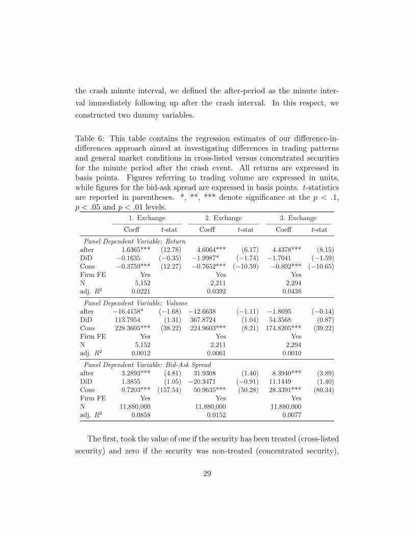
the crash minute interval, we defined the after-period as the minute inter-
val immediately following up after the crash interval. In this respect, we
constructed two dummy variables.
Table 6: This table contains the regression estimates of our difference-in-differences approach aimed at investigating differences in trading patternsand general market conditions in cross-listed versus concentrated securitiesfor the minute period after the crash event. All returns are expressed inbasis points. Figures referring to trading volume are expressed in units,while figures for the bid-ask spread are expressed in basis points. t-statisticsare reported in parentheses. *, **, *** denote significance at the p < .1,p < .05 and p < .01 levels.
1. Exchange 2. Exchange 3. Exchange
Coeff t-stat Coeff t-stat Coeff t-stat
Panel Dependent Variable: Returnafter 1.6365*** (12.78) 4.6064*** (6.17) 4.4378*** (8.15)DiD −0.1635 (−0.35) −1.9987* (−1.74) −1.7041 (−1.59)Cons −0.3759*** (12.27) −0.7652*** (−10.59) −0.802*** (−10.65)Firm FE Yes Yes YesN 5,152 2,211 2,294adj. R2 0.0221 0.0392 0.0438
Panel Dependent Variable: Volumeafter −16.4158* (−1.68) −12.6638 (−1.11) −1.8695 (−0.14)DiD 113.7954 (1.31) 367.8724 (1.04) 54.3568 (0.87)Cons 228.3605*** (38.22) 224.9603*** (8.21) 174.8205*** (39.22)Firm FE Yes Yes YesN 5,152 2,211 2,294adj. R2 0.0012 0.0061 0.0010
Panel Dependent Variable: Bid-Ask Spreadafter 3.2893*** (4.81) 31.9308 (1.46) 8.3940*** (3.89)DiD 1.3855 (1.05) −20.3471 (−0.91) 11.1449 (1.40)Cons 9.7203*** (157.54) 50.9635*** (50.28) 28.3391*** (80.34)Firm FE Yes Yes YesN 11,880,000 11,880,000 11,880,000adj. R2 0.0858 0.0152 0.0077
The first, took the value of one if the security has been treated (cross-listed
security) and zero if the security was non-treated (concentrated security),
29

while the second dummy variable took the value of one if the observation
belonged to the minute immediately following after to the crash minute and
zero otherwise. Using this experimental setting, we investigated potential
differences in observed returns, trading volume, and bid-ask spread patterns
between cross-listed and concentrated securities, for each of the three main
exchanges.
We observed that throughout all our model specifications the difference-
in-differences interaction term had statistically insignificant coefficients at
the p < .05 level (see Table 6). The panels depicted our dependent variables
(i.e., observed returns, trading volume, and bid-ask spread) in our regres-
sion equation. Weak evidence existed for different observed returns on the
secondary exchange between cross-listed and concentrated stocks after the
treatment (at the p < .1 significance level). The fact that, in general, the
interaction terms were insignificantly different from zero supports the view
that the development of market conditions and trading activity around the
crash interval is similar for cross-listed and concentrated securities. As an
additional robustness check, we reran our regressions after splitting our sam-
ple into terciles and found that the difference-in-differences interaction term
had statistically insignificant coefficients at the p < .05 throughout all model
specifications. This finding supports and complements the findings of O’Hara
and Ye (2011), who found that market fragmentation does not harm market
quality.
4. Conclusion
In this paper, we investigated the effects of market fragmentation and the
structure of intraday returns around extreme downward price movements. In
an event study, whereby following an exogenous external shock 45 Nasdaq100
constituents experienced an extreme concomitant negative price movement,
we investigated potential differences in market conditions and trading pat-
30

terns between cross-listed securities and stocks whose trading volume is con-
centrated on a single exchange. Using a difference-in-differences approach,
our results point towards similarities in trading activity and market condi-
tions of stocks with various degrees of market fragmentation. This finding
supports the idea that market fragmentation does not harm market quality.
Furthermore, we analyzed more than 46 million one-minute intervals of
the Nasdaq100 constituents in the period ranging from January 2014 to Jan-
uary 2019. We identified 15,242 extreme minute return intervals and further-
more found clear evidence supporting an after crash return reversal, which
is about 28% of the crash return.
These findings provided indications of market inefficiency around idiosyn-
cratic stock price crashes. High-frequency traders may exploit such market
overreactions by providing short-term liquidity in the minute after the stock
price crash occurs.
31

References
Ait-Sahalia, Y. and Saglam, M. (2017). High frequency market making:
Optimal quoting. SSRN Working.
Aitken, M., Chen, H., and Foley, S. (2017). The impact of fragmentation, ex-
change fees and liquidity provision on market quality. Journal of Empirical
Finance, 41:140–160.
Bessembinder, H. (2003). Quote-based competition and trade executioncosts
in NYSE-listed stocks. Journal of Financial Economics, 70:85–422.
Biais, B., Foucault, T., and Moinas, S. (2015). Equilibrium fast trading.
Journal of Financial Economics, 116(2):292–313.
Boehmer, E., Fong, K. Y. L., and Wu, J. (2018). Algorithmic trading and
market quality: International evidence. SSRN Working Paper.
Brogaard, J., Carrion, A., Moyaert, T., Riordan, R., Shkilko, A., and
Sokolov, K. (2018). High frequency trading and extreme price movements.
Journal of Financial Economics, 128(2):253–265.
Brogaard, J., Hendershott, T., and Riordan, R. (2014). High-frequency trad-
ing and price discovery. Review of Financial Studies, 27(8):2267–2306.
Brogaard, J., Hendershott, T., and Riordan, R. (2017). High frequency
trading and the 2008 short-sale ban. Journal of Financial Economics,
124(1):22–42.
Budish, E., Cramton, P., and Shim, J. (2015). The high-frequency trading
arms race: Frequent batch auctions as a market design response. Quarterly
Journal of Economics, 130(4):1547–1621.
Callaway, B., Li, T., and Oka, T. (2018). Quantile treatment effects in
difference in differences models under dependence restrictions and with
only two time periods. Journal of Econometrics, 206(2):395–413.
32

Carrion, A. (2013). Very fast money: High-frequency trading on the NAS-
DAQ. Journal of Financial Markets, 16:680–711.
Chaboud, A. P., Chiquoine, B., Hjalmarsson, E., and Vega, C. (2014). Rise of
the machines: Algorithmic trading in the foreign exchange market. Journal
of Finance, 69:2045–2084.
Chordia, T., Roll, R., and Subrahmanyam, A. (2001). Market liquidity and
trading activity. Journal of Finance, 56(2):501–530.
Chordia, T., Roll, R., and Subrahmanyam, A. (2008). Liquidity and market
efficiency. Journal of Financial Economics, 87:249–268.
Foucault, T., Roell, A., and Sandas, P. (2003). Market making with costly
monitoring: An analysis of the SOES controversy. Review of Financial
Studies, 16(2):345–384.
Gao, C. and Mizrach, B. (2016). Market quality breakdowns in equities.
Journal of Financial Markets, 28:1–23.
Hameed, A. and Mian, G. M. (2015). Industries and stock return reversals.
Journal of Financial and Quantitative Analysis, 50(1/2):89–117.
Handa, P. and Schwarz, R. A. (1993). Limit order trading. Journal of
Finance, 51(5):1835–1861.
Hasbrouck, J. (2018). High-frequency quoting: Short-term volatility in bids
and offers. Journal of Financial and Quantitative Analysis, 53(2):613–641.
Hasbrouck, J. and Saar, G. (2013). Low-latency trading. Journal of Financial
Markets, 16:646–679.
Hasbrouck, J. and Sofianos, G. (1993). The trades of market makers: An
empirical analysis of NYSE specialists. Journal of Finance, 48(5):1656–
1593.
33

Holden, C. W. and Jacobsen, S. (2014). Liquidity measurement problems
in fast, competitive markets: Expensive and cheap solutions. Journal of
Finance, 69(4):1747–1785.
Hutton, A. P., Marcus, A. J., and Tehranian, H. (2009). Opaque financial
reports, r2, and crash risk. Journal of Financial Economics, 94:67–86.
Jovanovic, B. and Menkveld, A. J. (2016). Middlemen in limit order markets.
SSRN Working Paper.
Kirilenko, A., Kyle, A. S., Samadi, M., and Tuzun, T. (2017). The flash
crash: High-frequency trading in an electronic market. Journal of Finance,
72(3):967–998.
Korajczyk, R. A. and Murphy, D. (2018). High frequency market making to
large institutional trades. Review of Financial Studies, 32:1034–1067.
Lee, C. M. C. and Ready, M. J. (1991). Inferring trade direction from intraday
data. Journal of Finance, 66(2):733–746.
Madhavan, A. and Smidt, S. (1993). An anlaysis of changes in specialist
inventories and quotations. Journal of Finance, 48(5):1595–1628.
Menkveld, A. J. and Zoican, M. A. (2017). Need for speed? Exchange latency
and liquidity. Review of Financial Studies, 30(4):1188–1228.
Nagel, S. (2012). Evaporating liquidity. Review of Financial Studies,
25(7):2005–2039.
O’Hara, M. and Ye, M. (2011). Is market fragmentation harming market
quality? Journal of Financial Economics, 100(3):459–474.
Shkilko, A. and Sokolov, K. (2020). Every cloud has a silver lining: Fast
trading, microwave connectivity, and trading cost. Journal of Finance,
forthcoming.
34

So, E. and Wang, S. (2014). News-driven return-reversals: Liquidity provi-
sion ahead of earnings announcements. Journal of Financial Economics,
114:20–35.
Upson, J. and VanNess, R. A. (2017). Multiple markets, algorithmic trading,
and market liquidity. Journal of Financial Markets, 32:49–68.
van Kervel, V. and Menkveld, A. J. (2019). High-frequncy trading around
large institutional orders. Journal of Finance, 74(3):1091–1137.
35

Appendix
Table 7: Complete list of variables and their corresponding descriptionVariable Name Variable Description
BidAsk The average observed bid-ask spread within a minute interval measuredin basis points.
Crash Dummy variable which identifies minute intervals with an extreme neg-ative return. The variable takes the value 1 if the condition listed underEquation (1) is fulfilled
MaxRet The maximum return, in basis points, observed between individualtrades taking place within the minute intervals.
MinRet The minimum return, in basis points, observed between individualtrades taking place within the minute intervals.
Mom The momentum observed up until the start of the current minute in-terval. It is calculated as the count of successive intervals during whichnegative (positive) realized returns are observed. For example, if neg-ative returns are observed in intervals t−3, t−2 and t−1, the value ofthe momentum variable for interval t will be −3. Symmetrically, if theseries of interval returns is positive, the momentum indicator will takethe value of +3. Alternatively, if we observe negative returns in inter-vals t−3 and t−1 but a positive return in interval t−2, the momentumindicator for interval t will be 0 as a sign change has been recorded.
LRQty The net number, expressed in thousands of units, of buyer/seller initi-ated trades. The value is calculated as the number of buyer initiatedtrades minus the number of seller initiated trades. Trades are catego-rized using the algorithm presented in Lee and Ready (1991).
NrTrd The number of trades recorded during a defined minute interval.
Ret The return, in basis points, observed in a minute interval, calculated asthe natural logarithm of the last trade price divided by the first tradeprice within a minute interval.
SD The standard deviation, in basis points, of the returns observed betweenindividual trades taking place within the minute intervals.
Vol The number of units, in thousands, of common stock traded during aminute interval.
36

Table 8: Description of quote conditions which have been excluded in linewith Holden and Jacobsen (2014), as well as the equity symbol suffixes forwhich observations from the daily trades dataset have not been included inour final sample
Quote Condition Description
A This condition indicates that the current offer is in ‘Slow’ quote mode.While in this mode, autoexecution is not eligible on the Offer side andcan be traded through pursuant to anticipated Regulation NMS require-ments
B This condition indicates that the current bid is in ‘Slow’ quote mode.While in this mode, autoexecution is not eligible on the Bid side andcan be traded through pursuant to anticipated Regulation NMS require-ments.
H This condition indicates that the quote is a ‘Slow’ quote on both the Bidand Offer sides. While in this mode, auto-execution is not eligible onthe Bid and Offer sides, and either or both sides can be traded throughpursuant to anticipated Regulation NMS requirements.
O This condition can be disseminated to indicate that this quote was theopening quote for a security for that Participant.
R This condition is used for the majority of quotes to indicate a normaltrading environment. It is also used by the FINRA Market Makers inplace of Quote Condition ‘O’ to indicate the first quote of the day fora particular security. The condition may also be used when a MarketMaker re-opens a security during the day.
W This quote condition is used to indicate that the quote is a Slow Quoteon both the Bid and Offer sides due to a Set Slow List that includesHigh Price securities. While in this mode, auto-execution is not eligible,the quote is then considered Slow on the Bid and Offer sides and eitheror both sides can be traded through, as per Regulation NMS.
Equity Suffix Description
K Non-Voting Shares
L Miscellaneous situations such as certificates of participation, preferredparticipation, and stubs
V Denotes a transaction in a security authorized for issuance, but not yetissued. All “when issued” transactions are on an “if” basis, to be settledif and when the actual security is issued.
Z Miscellaneous situations such as certificates of preferred when issued
37
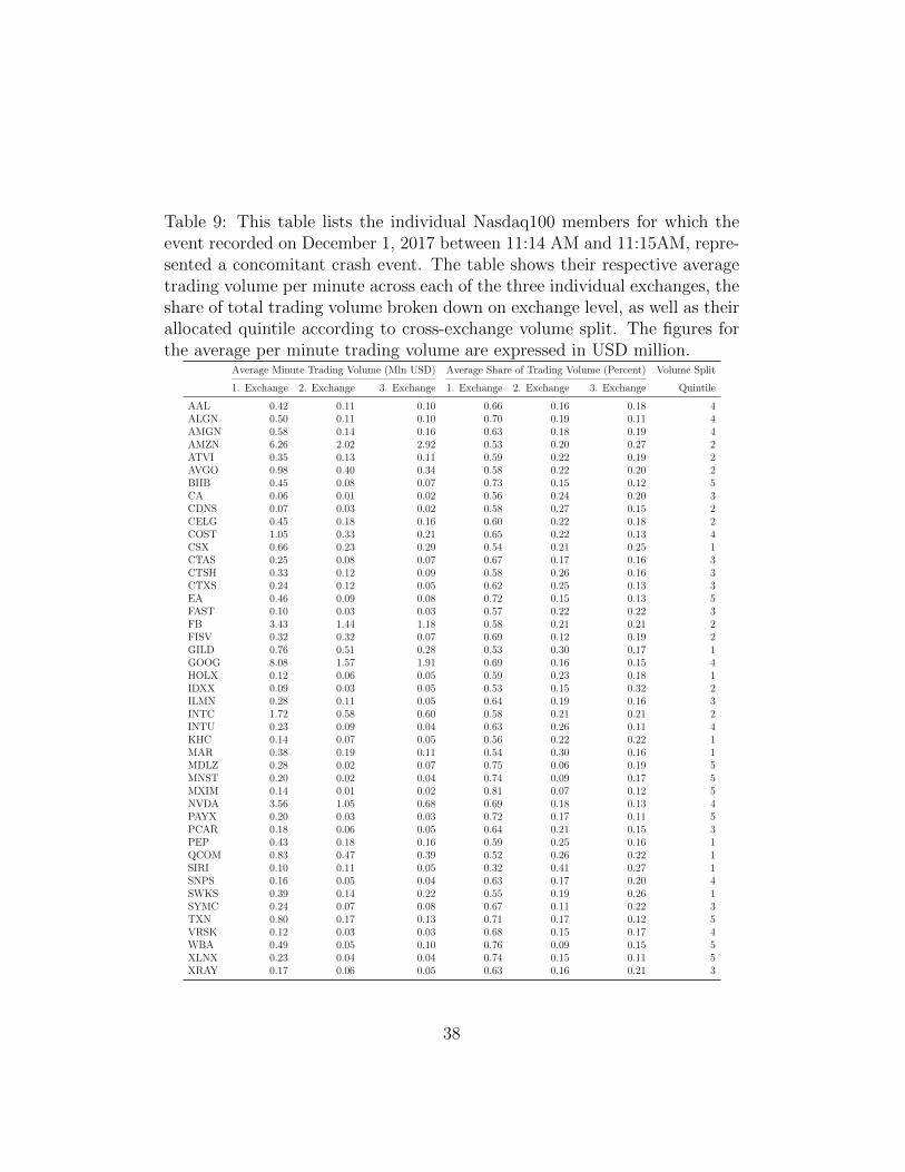
Table 9: This table lists the individual Nasdaq100 members for which theevent recorded on December 1, 2017 between 11:14 AM and 11:15AM, repre-sented a concomitant crash event. The table shows their respective averagetrading volume per minute across each of the three individual exchanges, theshare of total trading volume broken down on exchange level, as well as theirallocated quintile according to cross-exchange volume split. The figures forthe average per minute trading volume are expressed in USD million.
Average Minute Trading Volume (Mln USD) Average Share of Trading Volume (Percent) Volume Split
1. Exchange 2. Exchange 3. Exchange 1. Exchange 2. Exchange 3. Exchange Quintile
AAL 0.42 0.11 0.10 0.66 0.16 0.18 4ALGN 0.50 0.11 0.10 0.70 0.19 0.11 4AMGN 0.58 0.14 0.16 0.63 0.18 0.19 4AMZN 6.26 2.02 2.92 0.53 0.20 0.27 2ATVI 0.35 0.13 0.11 0.59 0.22 0.19 2AVGO 0.98 0.40 0.34 0.58 0.22 0.20 2BIIB 0.45 0.08 0.07 0.73 0.15 0.12 5CA 0.06 0.01 0.02 0.56 0.24 0.20 3CDNS 0.07 0.03 0.02 0.58 0.27 0.15 2CELG 0.45 0.18 0.16 0.60 0.22 0.18 2COST 1.05 0.33 0.21 0.65 0.22 0.13 4CSX 0.66 0.23 0.29 0.54 0.21 0.25 1CTAS 0.25 0.08 0.07 0.67 0.17 0.16 3CTSH 0.33 0.12 0.09 0.58 0.26 0.16 3CTXS 0.24 0.12 0.05 0.62 0.25 0.13 3EA 0.46 0.09 0.08 0.72 0.15 0.13 5FAST 0.10 0.03 0.03 0.57 0.22 0.22 3FB 3.43 1.44 1.18 0.58 0.21 0.21 2FISV 0.32 0.32 0.07 0.69 0.12 0.19 2GILD 0.76 0.51 0.28 0.53 0.30 0.17 1GOOG 8.08 1.57 1.91 0.69 0.16 0.15 4HOLX 0.12 0.06 0.05 0.59 0.23 0.18 1IDXX 0.09 0.03 0.05 0.53 0.15 0.32 2ILMN 0.28 0.11 0.05 0.64 0.19 0.16 3INTC 1.72 0.58 0.60 0.58 0.21 0.21 2INTU 0.23 0.09 0.04 0.63 0.26 0.11 4KHC 0.14 0.07 0.05 0.56 0.22 0.22 1MAR 0.38 0.19 0.11 0.54 0.30 0.16 1MDLZ 0.28 0.02 0.07 0.75 0.06 0.19 5MNST 0.20 0.02 0.04 0.74 0.09 0.17 5MXIM 0.14 0.01 0.02 0.81 0.07 0.12 5NVDA 3.56 1.05 0.68 0.69 0.18 0.13 4PAYX 0.20 0.03 0.03 0.72 0.17 0.11 5PCAR 0.18 0.06 0.05 0.64 0.21 0.15 3PEP 0.43 0.18 0.16 0.59 0.25 0.16 1QCOM 0.83 0.47 0.39 0.52 0.26 0.22 1SIRI 0.10 0.11 0.05 0.32 0.41 0.27 1SNPS 0.16 0.05 0.04 0.63 0.17 0.20 4SWKS 0.39 0.14 0.22 0.55 0.19 0.26 1SYMC 0.24 0.07 0.08 0.67 0.11 0.22 3TXN 0.80 0.17 0.13 0.71 0.17 0.12 5VRSK 0.12 0.03 0.03 0.68 0.15 0.17 4WBA 0.49 0.05 0.10 0.76 0.09 0.15 5XLNX 0.23 0.04 0.04 0.74 0.15 0.11 5XRAY 0.17 0.06 0.05 0.63 0.16 0.21 3
38

Chapter IIMarket Conditions of Cross-listed Securities
around a Macro Event
Alexandru Rif
Abstract
This paper investigates the developments in liquidity, trading costsand trading activity within individual cross-listed securities around amacro-economic event which triggered a concomitant three sigma neg-ative return for 71 Nasdaq100 constituents. The results strengthen theposition of a security’s primary exchange as liquidity forerunner. Theshare of “trade-through” volume, i.e. trades executed below the na-tional best bid or above the national best ask is higher for stocks withhigher volume concentration on a single exchange, suggesting thatmarket fragmentation is associated with increased market efficiency.Moreover, the reported share of “trade-through” volume, calculatedusing a one-millisecond time window, scrutinizes the current method-ology set forth under Rule 611 of the SEC’s National Market SystemRegulation.
JEL classification: G10, G12, G14.
Keywords : Market Fragmentation, Order Protection Rule, Trade-throughRule.

List of Figures
1 . . . . . . . . . . . . . . . . . . . . . . . . . . . . . . . . . . . 47
2 . . . . . . . . . . . . . . . . . . . . . . . . . . . . . . . . . . . 52
List of Tables
1 . . . . . . . . . . . . . . . . . . . . . . . . . . . . . . . . . . . 51
2 . . . . . . . . . . . . . . . . . . . . . . . . . . . . . . . . . . . 54
3 . . . . . . . . . . . . . . . . . . . . . . . . . . . . . . . . . . . 58
4 . . . . . . . . . . . . . . . . . . . . . . . . . . . . . . . . . . . 62
5 . . . . . . . . . . . . . . . . . . . . . . . . . . . . . . . . . . . 63
6 . . . . . . . . . . . . . . . . . . . . . . . . . . . . . . . . . . . 65
7 . . . . . . . . . . . . . . . . . . . . . . . . . . . . . . . . . . . 67
8 . . . . . . . . . . . . . . . . . . . . . . . . . . . . . . . . . . . 68
9 . . . . . . . . . . . . . . . . . . . . . . . . . . . . . . . . . . . 75
10 . . . . . . . . . . . . . . . . . . . . . . . . . . . . . . . . . . . 76
11 . . . . . . . . . . . . . . . . . . . . . . . . . . . . . . . . . . . 77
12 . . . . . . . . . . . . . . . . . . . . . . . . . . . . . . . . . . . 78
13 . . . . . . . . . . . . . . . . . . . . . . . . . . . . . . . . . . . 79
14 . . . . . . . . . . . . . . . . . . . . . . . . . . . . . . . . . . . 80
15 . . . . . . . . . . . . . . . . . . . . . . . . . . . . . . . . . . . 81
16 . . . . . . . . . . . . . . . . . . . . . . . . . . . . . . . . . . . 82
17 . . . . . . . . . . . . . . . . . . . . . . . . . . . . . . . . . . . 83
40
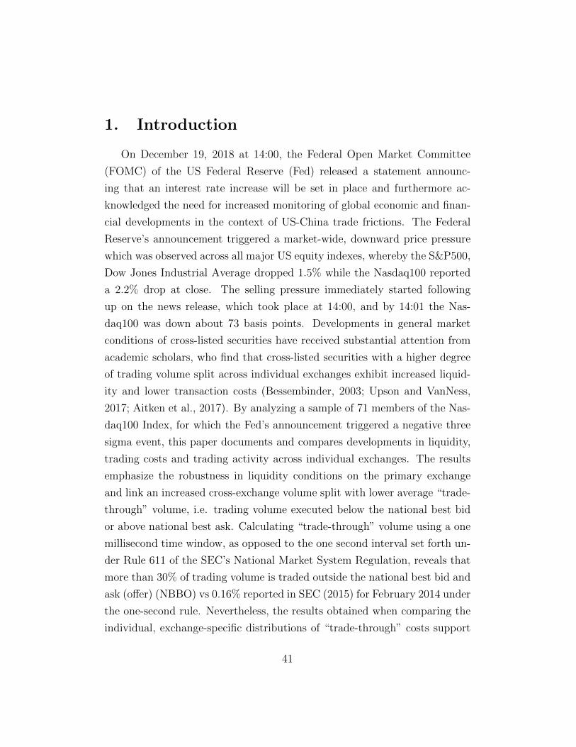
1. Introduction
On December 19, 2018 at 14:00, the Federal Open Market Committee
(FOMC) of the US Federal Reserve (Fed) released a statement announc-
ing that an interest rate increase will be set in place and furthermore ac-
knowledged the need for increased monitoring of global economic and finan-
cial developments in the context of US-China trade frictions. The Federal
Reserve’s announcement triggered a market-wide, downward price pressure
which was observed across all major US equity indexes, whereby the S&P500,
Dow Jones Industrial Average dropped 1.5% while the Nasdaq100 reported
a 2.2% drop at close. The selling pressure immediately started following
up on the news release, which took place at 14:00, and by 14:01 the Nas-
daq100 was down about 73 basis points. Developments in general market
conditions of cross-listed securities have received substantial attention from
academic scholars, who find that cross-listed securities with a higher degree
of trading volume split across individual exchanges exhibit increased liquid-
ity and lower transaction costs (Bessembinder, 2003; Upson and VanNess,
2017; Aitken et al., 2017). By analyzing a sample of 71 members of the Nas-
daq100 Index, for which the Fed’s announcement triggered a negative three
sigma event, this paper documents and compares developments in liquidity,
trading costs and trading activity across individual exchanges. The results
emphasize the robustness in liquidity conditions on the primary exchange
and link an increased cross-exchange volume split with lower average “trade-
through” volume, i.e. trading volume executed below the national best bid
or above national best ask. Calculating “trade-through” volume using a one
millisecond time window, as opposed to the one second interval set forth un-
der Rule 611 of the SEC’s National Market System Regulation, reveals that
more than 30% of trading volume is traded outside the national best bid and
ask (offer) (NBBO) vs 0.16% reported in SEC (2015) for February 2014 under
the one-second rule. Nevertheless, the results obtained when comparing the
individual, exchange-specific distributions of “trade-through” costs support
41

the idea that the US market performs as a unitary, integral market, whereby
the individual exchanges serve as access points for market participants.
Patterns in trading activity and developments in market quality have re-
ceived substantial attention from scholars throughout the evolution of finan-
cial markets (Hasbrouck and Schwartz, 1988; Admati and Pfleiderer, 1988;
Chordia et al., 2011; Nagel, 2012). Similar to Scholtus et al. (2014) and Eren-
burg and Lasser (2009), who use macro-economic news to study the effects of
algorithmic trading on trading volume, bid-ask spread, volatility and order-
book depth, this paper investigates general market conditions and incurred
cost inefficiencies in cross-listed securities, observed during and around the
Fed’s announcement time. The regulatory environment surrounding trade
execution in the US is governed by the Securities Exchange Act of 1934,
which stipulates clearly the fiduciary duty of broker-dealers to ensure best
execution for their clients. In Europe, contemporary efforts in this direction
are led by the series of Markets in Financial Instruments Directive (MIFID)
regulations, whereby the recent MIFID II directly and more thoroughly ad-
dresses this topic, setting stricter rules for monitoring the best execution
policy. Specifically, investment firms are required to publish the top five
trading venues where client orders are executed, along with an analysis aimed
at providing transparency and enable monitoring of actual execution qual-
ity. Nevertheless, practices conflicting with set fiduciary duties have been
long documented and studied by scholars. To name an example, phenomena
like “Cream-skimming”, the process of dealers routing retail trading activity
to competing venues, have been long documented and studied by scholars
(Easley et al., 1996; Battalio, 1997; Bolton et al., 2016). However, such
practices remain beyond the scope of this work.
The return recorded in the minute following up to the Fed’s announcement
constituted a three sigma negative event for 71 of the Nasdaq100 titles, which
compose the sample for the analysis included in this paper. High frequency
data is sourced from the New York Stock Exchange Trade and Quote (TAQ)
42

daily files. The sample period covers an eleven minute time window, which
is divided into two symmetric pre- and post-event periods of five minutes, as
well as the one minute event period.
Particularly, this paper compares the spreads and incurred trading costs
across the top three public exchanges by daily trading volume for individual
stocks, members in the Nasdaq100 Index, which exhibited an extreme down-
ward price movement in the first trading minute (14:00-14:01) following up
to the FOMC’s public announcement. In line with the findings in Brogaard
et al. (2018), sharp increases in trading activity, in particular dollar trading
volume and number of trades is reported. Similar to Chordia et al. (2002),
a deterioration in liquidity conditions, as measured by the quoted bid-ask
spread, is documented across all three covered individual exchanges. Despite
an increase of 218% in quoted bid-ask spread versus the pre-event period, the
primary exchange outperforms its peers when considering the absolute time
it was quoting prices in line with the national best bid or national best ask.
Specifically, quoting 69.86% in line with the national best bid and 68.85%
of the time with the national best ask, respectively, the primary exchange
offered the best buying and selling conditions throughout the event minute.
Calculating the percent of total volume executed on an individual exchange,
while set exchange was quoting prices below the national best bid or above
the national best ask at a 1 millisecond time window, reveals that about 30%
of trading volume across all exchanges would be classified as “trade-through”
volume vs. 0.16% reported by SEC (2015) for February 2014. Rule 611 of
SEC Regulation NMS expressly prohibits such practices, yet, in contrast,
classifies a trade as a “trade-through” using a more permissive one-second
time window. Kolmogorov-Smirnov tests are performed pairwise in order
to compare the individual distributions of incurred trade cost inefficiencies
on the individual exchanges. The results support the concept of the US
markets comprising a single virtual trading space with individual exchanges
acting as access points and complement the findings of O’Hara and Ye (2011),
43

who report that market fragmentation does not hinder general market qual-
ity. Moreover, in line with extant crash literature the results document and
confirm sharp increases in trading volume, quoted spread and number of ex-
ecuted trades when compared to the five minute pre-event and post-event
period (Brogaard et al., 2018).
Given its scope, this paper resides within, and contributes to, two major
literature streams covering market fragmentation and crash trading. Consid-
ering the current market architecture, which is comprised of multiple single
exchanges on which cross-listed stocks are actively traded by market partic-
ipants, market fragmentation bears fundamental implications on the general
market ecosystem and market conditions. Consequently, market fragmenta-
tion and, more narrowly, its implications on general market conditions, is
a topic that received significant attention by research scholars. Upson and
VanNess (2017) investigate the effect of cross-exchange quote competition on
national best bid and ask (offer) (NBBO) depth, trade execution, as well as
market fragmentation. They report that quote competition erodes NBBO
depth on individual exchanges, yet find that increased volume fragmentation
has a beneficial effect on both trade execution and general NBBO depth.
Aitken et al. (2017) link increasing degrees of fragmentation with improved
market quality. Similarly, Bessembinder (2003) show that competition be-
tween exchanges is associated with lower transaction costs and increased
liquidity.
The paper is structured as follows: Section 2 covers the theoretical frame-
work, Section 3 discusses the sample selection and data, Section 4 reports on
the analysis and main results, while Section 5 covers the conclusion.
44

2. Theoretical Framework
2.1. The Fed’s Announcement
Chen et al. (1986) where amongst the first scholars to empirically show
that stock returns react to macro-economic news announcements. Chris-
tiansen and Ranaldo (2007) report a significant impact of macro announce-
ments on correlations between stocks and bonds.
Modern economic theory and a deep field of literature have documented
the close relationship between the Federal Reserve’s interest rate target and
stock market reactions and impact on valuations (Campbell, 1987; Fama,
1981; Elyasiani and Mansur, 1998; Bjørnland and Leitemo, 2009). Rising
interest rates are used by market participants as signals of the economic
cycle (Chen, 2009), govern portfolio allocations (Boubaker et al., 2018) and
trigger higher discounts in company valuations (Flannery and James, 1984).
Chen (1991) documents the association between short term interest rates and
economic growth. Chulia et al. (2010) find that a 10bp interest rate increase
surprise is associated with a −46bp stock market return. Kontonikas et al.
(2013) report that stocks exhibit positive returns when the Fed cuts interest
rates, associating a 100bp interest rate cut with a 400bp positive reaction in
the S&P500 Index.
At the time of the announcement, the Fed acknowledged the deteriorating
financial outlook caused by the escalating trade frictions between the United
States and China, and also confirmed in the published FOMC Meeting notes
the rising concerns among market participants of a potential economic slow-
down.
This event constituted a fundamental economic shock, triggering an im-
mediate negative reaction throughout the US stock markets. Of all the 100
Nasdaq constituents, the event represented a three sigma event for 71 ti-
tles. The method used for identifying and cataloging the trading minute
following up to the Fed’s announcement is in line with the methodology set
45

forth in Rif and Utz (2019). Specifically, two methodologies of identifying
extreme returns were used. The first, uses rolling average minute returns
and minute return standard deviation, while the second relies on matched
average minute returns and minute return standard deviations for identifying
extreme negative returns.
The identification procedure is formalized in Equation 1
rt ≤ µt − 3.19 × σt (1)
Various time intervals were used for both identification methodologies,
corresponding to one week, one month, one quarter and one year time spans.
The selected event minute, was identified concomitantly by both methodolo-
gies and across all previously mentioned time spans, as an extreme event for
all of the 71 Nasdaq100 titles.
Given its economic implication and magnitude, the Fed’s announcement
offers a valuable setting for studying the impact of a market wide negative
shock on general market conditions.
2.2. Market fragmentation
Increasing market fragmentation is a well documented phenomenon, whereby
newly established, highly-automated, electronic exchanges such as BATS are
gaining increasing market share (Menkveld, 2013). Figure 1 illustrates the
trend towards fragmentation as revealed by a study published by the SEC in
2015. Acting on its tripartite mission to protect investors, maintain fair and
orderly efficient markets, as well as to facilitate capital formation, the SEC
launched a series of proposals aimed at tackling the potential adverse effects
of market fragmentation (Stoll, 2001).
Regulation National Market System (NMS), passed by the SEC and
in force since 2005, directly addresses potential issues arising in a multi-
exchange set-up. It comprises of four main pillars, targeting fair trade ex-
46
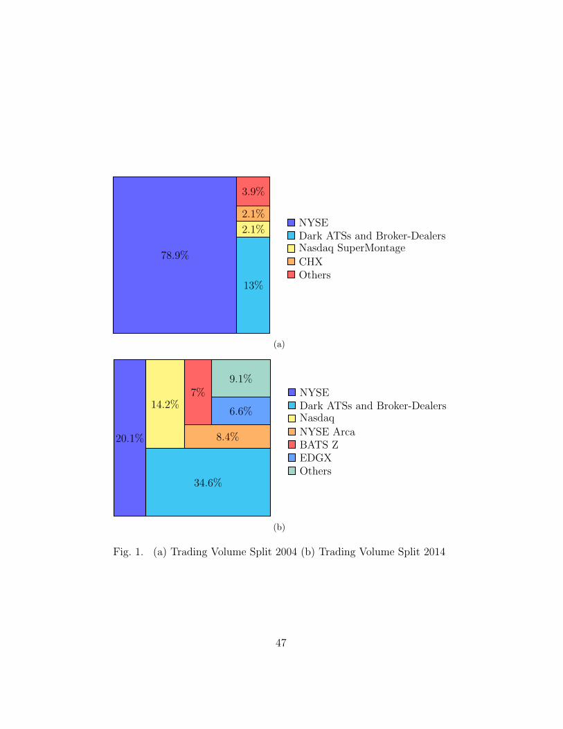
78.9%
13%
2.1%
2.1%
3.9%
NYSEDark ATSs and Broker-DealersNasdaq SuperMontage
CHXOthers
(a)
20.1%
34.6%
14.2%
8.4%
7%
6.6%
9.1%
NYSEDark ATSs and Broker-DealersNasdaq
NYSE ArcaBATS ZEDGXOthers
(b)
Fig. 1. (a) Trading Volume Split 2004 (b) Trading Volume Split 2014
47

ecution prices, inter-exchange access, minimum quotation increments and
improved market data access (SEC, 2005). Specifically, NMS Rule 611, also
referred to as “Order Protection Rule” or “Trade-through Rule” stipulates
that no trade is to be executed at prices which are inferior to bid and ask
prices readily available and accessible on other exchanges. In essence, the
rule effectively prohibits broker-dealers from executing trades on behalf of
their clients on a particular exchange, if the price at which the transaction
would be executed is below the national best bid or above the national best
ask. Nevertheless, exceptions are also stipulated.
Paragraph (b)(8) of Rule 611 provides for an exception in the case of
“flickering” quotations. Namely, it exempts from this rule situations, where
the exchange on which the potential “trade-through” took place quoted dur-
ing the previous one-second time window, prices in line with the national
best bid or national best ask, which were in line or worse than the trans-
acted price. The disclosed reasoning behind this exception is to provide a
so-called “workable” protection system, which is not imposing an excessive
burden on the exchange’s order routing operations in times of fast changing
market prices.(SEC, 2005)
Another important exception concerning Inter-Market Sweep Orders (ISOs)
is also foreseen under Paragraphs (b)(5) and (b)(6) of Rule 611. These or-
ders are exempt from the effects of the “Order Protection Rule” and once
a qualified ISO is received by an exchange, it is warranted to go ahead and
process that order without having the need to check for protected quotations
on other exchanges. (SEC, 2005) Moreover, Pargraph (b)(7) of Rule 611 also
exempts benchmark orders from the “Order Protection Rule”.
A memorandum published in April 2015 by the SEC, presents the im-
pact that Regulations NMS and, specifically, Rule 611 has had on reducing
“trade-through” volume. The memorandum shows that, as of February 2014,
0.16% of the total trading volume on the Nasdaq qualified as “trade-through”
volume, as opposed to 7.7% in February 2004. A similar pattern is also ex-
48
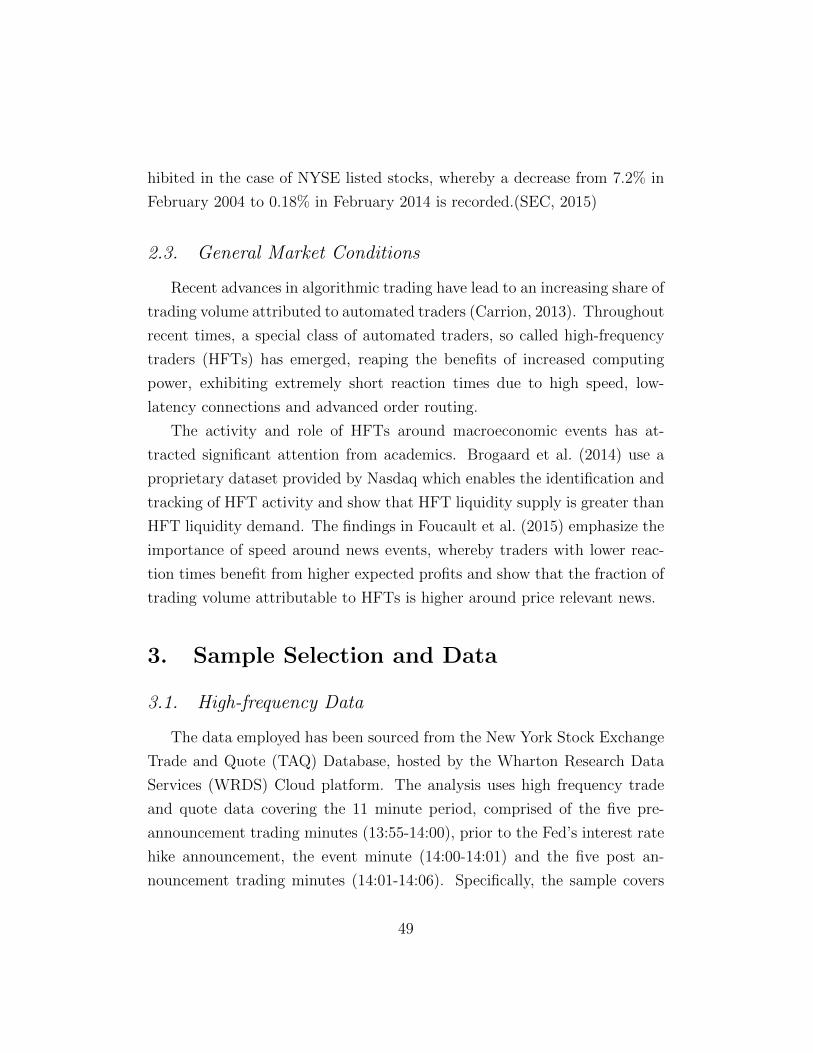
hibited in the case of NYSE listed stocks, whereby a decrease from 7.2% in
February 2004 to 0.18% in February 2014 is recorded.(SEC, 2015)
2.3. General Market Conditions
Recent advances in algorithmic trading have lead to an increasing share of
trading volume attributed to automated traders (Carrion, 2013). Throughout
recent times, a special class of automated traders, so called high-frequency
traders (HFTs) has emerged, reaping the benefits of increased computing
power, exhibiting extremely short reaction times due to high speed, low-
latency connections and advanced order routing.
The activity and role of HFTs around macroeconomic events has at-
tracted significant attention from academics. Brogaard et al. (2014) use a
proprietary dataset provided by Nasdaq which enables the identification and
tracking of HFT activity and show that HFT liquidity supply is greater than
HFT liquidity demand. The findings in Foucault et al. (2015) emphasize the
importance of speed around news events, whereby traders with lower reac-
tion times benefit from higher expected profits and show that the fraction of
trading volume attributable to HFTs is higher around price relevant news.
3. Sample Selection and Data
3.1. High-frequency Data
The data employed has been sourced from the New York Stock Exchange
Trade and Quote (TAQ) Database, hosted by the Wharton Research Data
Services (WRDS) Cloud platform. The analysis uses high frequency trade
and quote data covering the 11 minute period, comprised of the five pre-
announcement trading minutes (13:55-14:00), prior to the Fed’s interest rate
hike announcement, the event minute (14:00-14:01) and the five post an-
nouncement trading minutes (14:01-14:06). Specifically, the sample covers
49

trade and quote data for a basket of 71 companies included in the Nasdaq100
Index.
The consolidated NYSE TAQ Files contain nanosecond level trade and
quote data for each of the 14 participating facilities, as well as reconstructed
national best bid and offer data compiled by WRDS, based on the raw quote
data. Table 1 summarizes the trading activity in terms of volume and number
of trades recorded on December 19, 2018 split by each of the 14 participating
facilities.
It is important to note that trade observations for which the exchange
identifier refers to the Financial Ind. Regulatory Authority, Inc. are not
recorded by an actual exchange, but are trades reported by the FINRA Trade
Reporting Facility. For the most part, these are trades that were executed in
dark pools, directly between counter-parties or on various other platforms.
These observations are not considered, as no bid or ask data is available for
these trades, rendering impossible any liquidity related insights or deeper
analysis.
In line with the aim of the paper, the analysis focuses on the top three
public exchanges, ranked by trading volume, on which the 71 companies
are cross-listed. Specifically, the analysis focuses on data reported by Nas-
daq Stock Exchange, Bats BZX Exchange and NYSE Arca which together
account for 44.69% of the total dollar trading volume (68.19% exclusively
considering the public exchanges), as well as for 56.32% of the total number
of executed trades (68.56% exclusively considering the public exchanges).
3.2. Algorithmic Design
One of the main challenges when analyzing intra-day data is working with
data files of increased size. As an illustrative example, given a typical TAQ
Daily Quote file ranges from 30 to 50 gigabytes, screening for extreme intra-
day returns over a five year period implies iterating through approximately 50
petabytes or 50 million gigabytes. Implicitly, the magnitude of the resulting
50
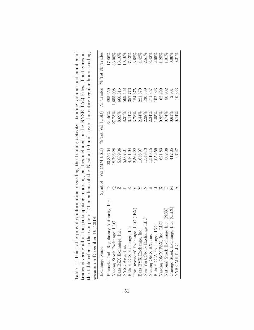
Tab
le1:
This
table
pro
vid
esin
form
atio
nre
gard
ing
the
trad
ing
acti
vit
y:
trad
ing
volu
me
and
num
ber
oftr
ades
cove
ring
all
ofth
epar
tici
pat
ing
rep
orti
ng
enti
ties
incl
uded
inth
eN
YSE
TA
QF
iles
.T
he
figu
res
inth
eta
ble
refe
rto
the
sam
ple
of71
mem
ber
sof
the
Nas
daq
100
and
cove
rth
een
tire
regu
lar
hou
rstr
adin
gse
ssio
non
Dec
emb
er19
,20
18.
Exch
ange
Nam
eS
ym
bol
Vol
(MM
US
D)
%T
otV
ol(U
SD
)N
rT
rad
es%
Tot
Nr
Tra
des
Fin
anci
alIn
d.
Reg
ula
tory
Au
thor
ity,
Inc.
D23
,356
.04
34.4
6%89
5,65
917
.86%
Nas
daq
Sto
ckE
xch
ange
,L
LC
Q18
,796
.28
27.7
3%1,
655,
098
33.0
0%B
ats
BZ
XE
xch
ange
,In
c.Z
5,88
9.06
8.69
%66
0,31
613
.16%
NY
SE
Arc
a,In
c.P
5,60
7.01
8.27
%50
9,43
810
.16%
Bat
sE
DG
XE
xch
ange
,In
c.K
4,16
1.94
6.14
%35
7,77
67.
13%
Th
eIn
vest
ors’
Exch
ange
,L
LC
(IE
X)
V2,
564.
223.
78%
184,
375
3.68
%B
ats
BY
XE
xch
ange
,In
c.Y
1,65
6.97
2.44
%22
1,57
04.
42%
New
Yor
kS
tock
Exch
ange
LL
CN
1,54
8.13
2.28
%13
0,88
92.
61%
Nas
daq
OM
XB
X,
Inc.
B1,
519.
152.
24%
171,
357
3.42
%B
ats
ED
GA
Exch
ange
,IN
CJ
1,05
2.59
1.55
%10
2,92
32.
05%
Nas
daq
OM
XP
SX
,In
c.L
LC
X62
1.83
0.92
%62
,499
1.25
%N
atio
nal
Sto
ckE
xch
ange
Inc.
(NS
X)
C50
2.08
0.74
%50
,902
1.01
%C
hic
ago
Sto
ckE
xch
ange
,In
c.(C
HX
)M
412.
050.
61%
2,90
10.
06%
NY
SE
MK
TL
LC
A97
.47
0.14
%10
,333
0.21
%
51
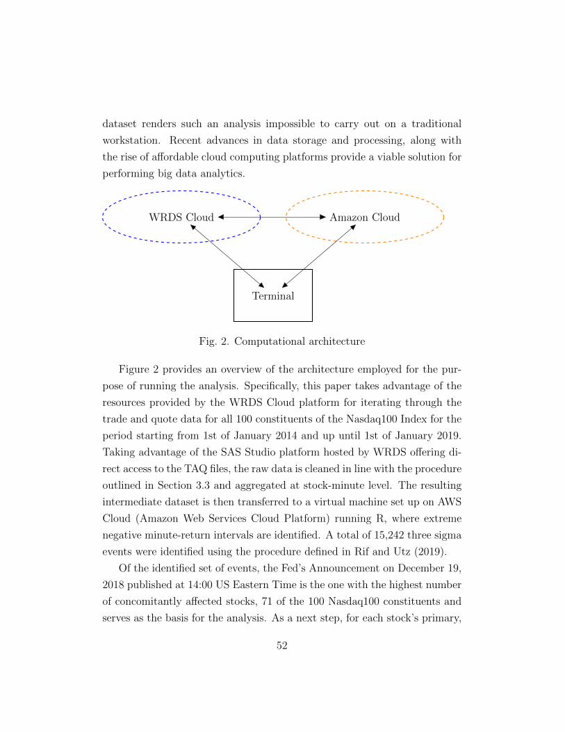
dataset renders such an analysis impossible to carry out on a traditional
workstation. Recent advances in data storage and processing, along with
the rise of affordable cloud computing platforms provide a viable solution for
performing big data analytics.
WRDS Cloud Amazon Cloud
Terminal
Fig. 2. Computational architecture
Figure 2 provides an overview of the architecture employed for the pur-
pose of running the analysis. Specifically, this paper takes advantage of the
resources provided by the WRDS Cloud platform for iterating through the
trade and quote data for all 100 constituents of the Nasdaq100 Index for the
period starting from 1st of January 2014 and up until 1st of January 2019.
Taking advantage of the SAS Studio platform hosted by WRDS offering di-
rect access to the TAQ files, the raw data is cleaned in line with the procedure
outlined in Section 3.3 and aggregated at stock-minute level. The resulting
intermediate dataset is then transferred to a virtual machine set up on AWS
Cloud (Amazon Web Services Cloud Platform) running R, where extreme
negative minute-return intervals are identified. A total of 15,242 three sigma
events were identified using the procedure defined in Rif and Utz (2019).
Of the identified set of events, the Fed’s Announcement on December 19,
2018 published at 14:00 US Eastern Time is the one with the highest number
of concomitantly affected stocks, 71 of the 100 Nasdaq100 constituents and
serves as the basis for the analysis. As a next step, for each stock’s primary,
52

secondary and tertiary exchange nanosecond level trade, quote and best bid
and ask data were retrieved for the event minute 14:00-14:01 as well as for
the five minute pre- and post-event periods through the WRDS in-house
developed Python package. Trade and quote data are matched at exchange
level, then snapshots of the top of the order book for each of the three
individual exchanges are generated and stored at a one-millisecond interval
for each stock. The analysis is then conducted using the resulting dataset.
3.3. Data Cleaning
The sample data is restricted to trades and quotes submitted to the in-
dividual exchanges during the time window starting from 13:55 and ending
at 14:06. First, any trade observations which are not referring to common
stock are excluded from the sample. Specifically, referring to the TAQ Client
specifications, any trades with conditions listed as A, B, H, K, L, O, R, V,
W, and Z are dropped from the dataset. Quote data is processed in line with
the methodology set forth in Holden and Jacobsen (2014) and Rif and Utz
(2019). Namely, quotes flagged with irregular trade conditions or any obser-
vations for which the bid and ask price stemming from the same reporting
venue are crossed are also dropped. Furthermore, observations for which ei-
ther the bid or the ask quantity are missing or listed as 0 are not considered.
Moreover, any trades for which the equity suffixes were listed as K, L , V,
or Z were also dropped from the dataset. Quote and trade data are matched
according to the procedure introduced in Holden and Jacobsen (2014). A
table covering the description of the excluded trade and quote conditions is
included in the Appendix.
Table 2 reports general summary statistics showing the individual de-
velopments in average minute return, bid-ask spread as well as the minute
trading volume split according to individual exchanges and covering the five
minute period prior to the Fed’s announcement, the event minute, and the
five minute period following up the publication of the announcement. All
53
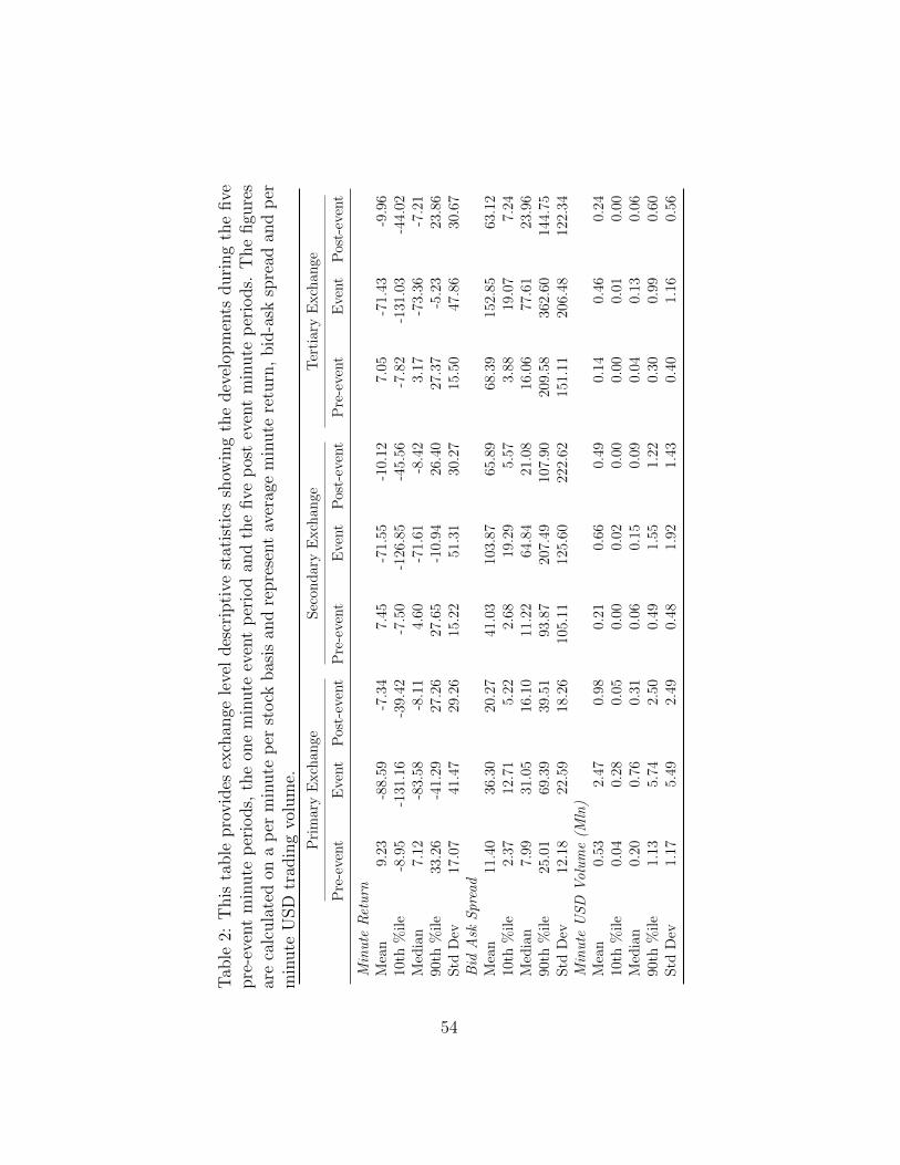
Tab
le2:
This
table
pro
vid
esex
chan
gele
vel
des
crip
tive
stat
isti
cssh
owin
gth
edev
elop
men
tsduri
ng
the
five
pre
-eve
nt
min
ute
per
iods,
the
one
min
ute
even
tp
erio
dan
dth
efive
pos
tev
ent
min
ute
per
iods.
The
figu
res
are
calc
ula
ted
ona
per
min
ute
per
stock
bas
isan
dre
pre
sent
aver
age
min
ute
retu
rn,
bid
-ask
spre
adan
dp
erm
inute
USD
trad
ing
volu
me.
Pri
mar
yE
xch
ange
Sec
ond
ary
Exch
ange
Ter
tiar
yE
xch
ange
Pre
-eve
nt
Eve
nt
Pos
t-ev
ent
Pre
-eve
nt
Eve
nt
Pos
t-ev
ent
Pre
-eve
nt
Eve
nt
Pos
t-ev
ent
Min
ute
Ret
urn
Mea
n9.
23-8
8.59
-7.3
47.
45-7
1.55
-10.
127.
05-7
1.43
-9.9
610
th%
ile
-8.9
5-1
31.1
6-3
9.42
-7.5
0-1
26.8
5-4
5.56
-7.8
2-1
31.0
3-4
4.02
Med
ian
7.12
-83.
58-8
.11
4.60
-71.
61-8
.42
3.17
-73.
36-7
.21
90th
%il
e33
.26
-41.
2927
.26
27.6
5-1
0.94
26.4
027
.37
-5.2
323
.86
Std
Dev
17.0
741
.47
29.2
615
.22
51.3
130
.27
15.5
047
.86
30.6
7B
idA
skS
prea
dM
ean
11.4
036
.30
20.2
741
.03
103.
8765
.89
68.3
915
2.85
63.1
210
th%
ile
2.37
12.7
15.
222.
6819
.29
5.57
3.88
19.0
77.
24M
edia
n7.
9931
.05
16.1
011
.22
64.8
421
.08
16.0
677
.61
23.9
690
th%
ile
25.0
169
.39
39.5
193
.87
207.
4910
7.90
209.
5836
2.60
144.
75S
tdD
ev12
.18
22.5
918
.26
105.
1112
5.60
222.
6215
1.11
206.
4812
2.34
Min
ute
US
DV
olu
me
(Mln
)M
ean
0.53
2.47
0.98
0.21
0.66
0.49
0.14
0.46
0.24
10th
%il
e0.
040.
280.
050.
000.
020.
000.
000.
010.
00M
edia
n0.
200.
760.
310.
060.
150.
090.
040.
130.
0690
th%
ile
1.13
5.74
2.50
0.49
1.55
1.22
0.30
0.99
0.60
Std
Dev
1.17
5.49
2.49
0.48
1.92
1.43
0.40
1.16
0.56
54

figures are calculated based on stock-minute figures.
The first panel, covering the minute returns, shows the magnitude of the
Fed announcement’s impact, whereby the average minute return across the
71 individual companies is -88.59bp in the case of the primary exchange,
while the average minute return within the five minute period prior to the
event which is 9.23bp. A similar profile is also displayed when considering the
figures for the secondary and tertiary exchanges, where the average return in
the pre-event period is 7.45bp and 7.05bp, respectively, while during the event
minute the average drop is reported at -71bp, 55bp and -71.43bp respectively,
roughly similar to the ratio exhibited on the primary exchange. Similarities
across the exchanges are also observed when considering the minute return
distributional data, whereby comparable figures are reported for the 10th and
90th decile, as well as for the median and standard deviation. It is important
to stress that these figures can very well vary across the individual trading
venues, since they are calculated based on actual trade prices as opposed to
quoted returns.
Coupling the return data with the volume data reported in the third
panel serves as primary indication that market participants are active and
exhibit similar trading activity across all three public exchanges. In line
with literature linking trading volume to price movements, (Brogaard et al.,
2018; Lee and Swaminathan, 2000) we observe that trading volume sharply
increased across all three exchanges during the event minute. The primary
exchange experiences a fivefold increase in minute-stock dollar trading vol-
ume, or $2.47 Mln per title, when compared with the average minute trading
volume during the pre-event period, $0.53 Mln per title. The secondary and
tertiary exchanges experience a threefold increase in minute trading volume
during the event minute, reaching $0.66 Mln and $0.46 Mln, compared to
$0.21 Mln and $0.14 Mln in the pre-event period. The minute volume post-
event is substantially lower throughout all exchanges and is roughly double
to the one recorded in the pre-event levels. The importance of the relatively
55

higher increase in trading volume experienced by the primary exchange, is
further augmented by the findings in Eun and Sabherwal (2003), who report
a direct link between the share of a cross-listed security’s total volume on
one exchange and the share of informative trades which augment the price
discovery process.
Referring to the second panel, the quoted bid-ask spread, differences
in liquidity level, proxied by the bid-ask spread, are observable across the
three exchanges throughout all three time periods. The first exchange, as
in the case of minute trading volume, exhibits the best trading conditions
when benchmarked against the other two exchanges, with the quoted bid-
ask spread being throughout all the periods smaller than that reported by
the counterparts. Noticeably, the distribution of the bid-ask spread is right-
skewed, with the values for the mean being considerably higher than the
median throughout all three exchanges and time periods. Nevertheless, even
when comparing the median bid-ask spread values for all exchanges, the pri-
mary exchange, remains the venue offering the best trading conditions.
A deterioration in trading conditions, i.e. an increase in the quoted spread
is exhibited by all three trading venues, whereby the mean bid-ask spread
quoted on the primary exchange increases from an average of 11.40bp during
the five pre-event minutes to 36.30bp during the event minute , represent-
ing a 218% increase and drops to 20.27bp in the post-event period. The
secondary and tertiary exchange, exhibit a similar pattern, quoting a mean
bid-ask spread of 41.03bp and 68.39bp, respectively for the five minute period
prior to the Fed’s announcement, while spiking to 103.87bp and 152.85bp,
respectively, during the event minute and leveling off at 65.89bp and 63.12bp
during the five post event minutes. These reported developments in the
quoted bid-ask spread are in line with Chordia et al. (2002) who document
a drop in liquidity in times of falling stock prices.
These initial figures stress the importance, for liquidity aware traders,
of having access to a security’s primary exchange. The following section
56

aims at shedding more light regarding the trading conditions on individual
exchanges.
4. Analysis and Main Results
4.1. Liquidity Conditions
In order to get a better picture of the liquidity, as proxied by the quoted
bid-ask spread, across the individual trading venues, Table 3 provides an
overview regarding the quoted bid and ask prices, by exchange, benchmarked
versus the national best bid (NBB) and national best ask (offer) price (NBO),
as well as benchmarked versus the other two trading venues. Specifically, the
figures illustrate the percentage of time during which each exchange was at
the national best bid or at the national best ask, across each of the three
time periods of focus, as well as the percentage of time during which the
individual exchange was deviating from the national best bid or ask, but
nevertheless, it was providing superior quotes in comparison to the other two
trading venues.
The first panel of Table 3 shows the percentage of time that each of the
individual exchanges is matching the national best bid. The figures for the
primary exchange confirm the results introduced already by the descriptive
statistics, whereby the primary exchange was quoting the most favorable
bid-ask spread, and show that the exchange is on average 70.45% of the time
matching the national best bid during the pre-event period. The secondary
and tertiary exchanges, on the other hand, score substantially lower during
the same period, at 47.90% and 38.07% respectively. Similar figures, stressing
the superiority of the primary exchange in terms of liquidity during the pre-
event period, are also reported in the third panel, the one referring to the
time during which an exchange is at the national best ask.
The most interesting development, constituting the main finding and a
strong argument for the supremacy of the primary exchange in terms of
57

Tab
le3:
This
table
show
sth
etr
adin
gco
ndit
ions
acro
ssth
epri
mar
y,se
condar
yan
dte
rtia
ryex
chan
ges,
split
acco
rdin
gto
the
thre
eti
me
per
iods
ofth
eF
ed’s
annou
nce
men
t:th
efive
min
ute
pre
-eve
nt
per
iod,
the
even
tm
inute
and
the
five
min
ute
pos
tev
ent
per
iod.
The
resu
lts
are
pre
sente
dse
par
atel
yfo
rbid
and
ask
pri
ces,
inor
der
tohig
hligh
tan
yp
oten
tial
effec
tsof
hig
hse
llin
gor
buyin
gpre
ssure
acro
ssth
eth
ree
diff
eren
tp
erio
ds
ofth
eev
ent.
Inor
der
toin
crea
setr
ansp
aren
cyan
den
able
ab
ette
rco
mpar
ison
amon
gst
the
thre
eex
chan
ges,
the
four
pan
els
also
split
the
resu
lts
bet
wee
nti
me
atnat
ional
bes
tbid
ornat
ional
bes
tas
k,
vers
us
tim
eb
elow
nat
ional
bes
tbid
(ab
ove
nat
ional
bes
tas
k)
but
abov
eth
eb
est
bid
(bel
owth
eb
est
ask)
quot
edon
the
other
two
com
pet
ing
exch
ange
s.A
llfigu
res
are
calc
ula
ted
ona
per
min
ute
-sto
ckav
erag
e.
Pri
mar
yE
xch
ange
Sec
ond
ary
Exch
ange
Ter
tiar
yE
xch
ange
Pre
-eve
nt
Eve
nt
Pos
t-ev
ent
Pre
-eve
nt
Eve
nt
Pos
t-ev
ent
Pre
-eve
nt
Eve
nt
Pos
t-ev
ent
%of
Tim
eat
nat
ion
albe
stbi
dM
ean
70.4
5%69
.86%
65.3
0%47
.90%
24.4
7%40
.36%
38.0
7%18
.19%
31.0
1%10
th%
ile
37.8
3%39
.61%
33.0
3%3.
95%
3.73
%5.
29%
3.54
%0.
51%
2.67
%M
edia
n73
.64%
72.2
8%67
.62%
49.9
7%22
.75%
39.2
3%33
.67%
11.6
5%25
.22%
90th
%il
e96
.56%
87.1
1%91
.91%
87.7
7%49
.87%
76.1
5%79
.34%
44.3
8%68
.50%
Std
Dev
22.4
4%18
.40%
22.1
2%29
.71%
17.0
7%25
.78%
27.4
6%18
.55%
24.5
3%%
ofT
ime
belo
wn
atio
nal
best
bid
but
abov
eot
her
exch
ange
sM
ean
7.59
%12
.10%
8.55
%2.
61%
1.43
%3.
29%
1.58
%1.
37%
1.64
%10
th%
ile
0.01
%1.
16%
0.11
%0.
00%
0.01
%0.
01%
0.00
%0.
00%
0.00
%M
edia
n1.
95%
10.6
5%3.
78%
0.36
%0.
27%
1.01
%0.
06%
0.38
%0.
25%
90th
%il
e21
.07%
24.7
6%20
.72%
6.80
%4.
44%
8.48
%5.
35%
3.77
%4.
28%
Std
Dev
13.3
1%10
.74%
13.0
6%6.
86%
2.35
%5.
89%
4.17
%2.
58%
3.95
%%
ofT
ime
atn
atio
nal
best
ask
Mea
n67
.81%
68.8
5%63
.15%
44.2
3%18
.60%
34.6
9%33
.27%
19.3
3%24
.65%
10th
%il
e34
.45%
42.5
2%31
.75%
3.37
%0.
45%
3.28
%2.
00%
0.34
%1.
35%
Med
ian
71.5
2%71
.39%
66.8
2%41
.59%
14.8
4%29
.72%
25.8
0%12
.44%
19.0
8%90
th%
ile
95.1
5%94
.78%
87.8
2%88
.22%
44.5
3%72
.39%
76.0
0%47
.82%
54.7
5%S
tdD
ev22
.93%
18.2
3%20
.89%
31.3
8%17
.11%
25.3
1%27
.96%
21.3
2%21
.76%
%of
Tim
eab
ove
nat
ion
albe
stas
kbu
tbe
low
othe
rex
chan
ges
Mea
n7.
86%
12.3
0%9.
16%
2.96
%1.
65%
4.13
%2.
70%
1.60
%2.
27%
Mea
n7.
86%
12.3
0%9.
16%
2.96
%1.
65%
4.13
%2.
70%
1.60
%2.
27%
10th
%il
e0.
01%
1.69
%0.
18%
0.00
%0.
00%
0.01
%0.
00%
0.01
%0.
01%
Med
ian
1.97
%10
.48%
4.84
%0.
69%
0.37
%1.
46%
0.17
%0.
23%
0.33
%90
th%
ile
22.9
7%22
.47%
23.1
3%9.
00%
5.97
%10
.52%
8.30
%5.
08%
6.75
%S
tdD
ev13
.13%
12.1
2%11
.66%
6.25
%2.
46%
8.11
%6.
32%
2.30
%4.
61%
58

liquidity during extreme events, refers to the trading conditions, during the
event minute. The primary exchange is slightly under 70% of the time at the
national best bid and 68.86% of the time at the national best ask, figures
which are only marginally below the figures reported by the primary exchange
for the pre-event period. In contrast, the magnitude of the deterioration from
the pre-event liquidity conditions, to those in the event minute, is significantly
higher in the case of the secondary and tertiary exchanges. The percent of
time during which these two venues are at the best bid are 24.47% and
18.19%, respectively, which represents a -48.90% and -52.20% relative drop
compared to the percent of time during which these exchanges were at the
best bid in the pre-event period. Similar developments are also reported
when referring to the percent of time during which the secondary and tertiary
exchanges are quoting ask prices in line with the national best ask during the
event minute. The secondary and tertiary exchanges are, on average 18.60%
and 19.33% of the time at the national best ask, representing a -58.01%
and -41.89% relative drop, respectively when benchmarked against pre-event
levels.
The stark deterioration in quoted spreads on the secondary and tertiary
exchanges is further augmented by the figures reported in panels 2 and 4.
Specifically, these figures show the percent of time during which an individual
exchange is quoting bid or ask prices which are inferior to the national best
bid or national best ask, yet better than the other 2 comparable venues. The
primary exchange quotes below national best bid yet superior to those on
the secondary and tertiary exchange, 7.59% of the time during the pre-event
period, while this figure increases up to 12.10% during the event minute.
On the other hand and in contrast to the developments on the primary
exchange, the secondary and tertiary exchange quote bid prices below the
national best bid but superior to their counterparts during 2.61% and 1.58%
of the time in the pre-event period, while these figures drop to 1.43% and
1.37%, respectively during the event minute. These developments further
59

show the superior trading conditions exhibited by the primary exchange.
It is important to note, that the developments in the quoted bid prices are
of particular interest, given that the event triggered a negative price reaction
and a substantial trading volume increase as reported in the previous section.
Indeed, the findings suggest, that market participants wishing to close or
reduce open positions would be in the best position to do so by having access
to the primary exchange. Adding the time during which each exchange is
at the national best bid or offer with the time during which the individual
exchange is superior to its counterparts further strengthens this argument.
Referring again to mean values, the primary exchange is an optimal selling
venue during 78.0% of the time during the pre-event period, while this figure
experiences an increase during the event minute to 81.96%. On the other
hand, the secondary and tertiary exchanges represent optimal selling venues
during 50.51% and 39.65% of the time during the pre-event period, while,
in contrast to the primary exchange, they experience a deterioration in this
metric in the event-period, providing only 25.90% and 19.56% of the time
optimal selling conditions.
Similar developments are also observed when focusing on optimal buying
conditions, as measured by the sum of time an individual exchange is at
the national best ask or, above the national best ask, yet below the ask price
quoted by its respective other two counterparts. The primary exchange again
dominates in terms of the total time it quotes optimal ask prices: 75.67%
of the time during the pre-event period, 81.15% during the event period
and 72.31% during the post-event period. In contrast, the secondary and
tertiary exchanges, report 47.19% and 35.97% ask price optimality during
the pre-event period, 20.25% and 20.93% during the event minute, 38.82%
and 26.92% during the post-event period. Consequently, assuming a mar-
ket participant would wish to open a position after the extreme downward
movement, would be best served on the primary exchange.
However, despite the more favorable conditions offered by the primary
60

exchange, as documented above, trades are nevertheless also taking place
on the secondary and tertiary exchanges. This introduces the second re-
search question: Are market participants that trade on secondary or tertiary
exchanges incurring additional trading costs?
4.2. Trade Price Inefficiencies and Trading Activity
In order to explore the market participant’s trading activity and uncover
any potential inefficiencies that might arise from a trader executing trades
on an exchange that deviates from the national best bid or offer, or on an
exchange that quotes inferior bid or ask prices to those on the other two
trading venues, we split the sample of 71 stocks into five quintiles, according
to their degree of cross-listing.
In line with the approach in Upson and VanNess (2017), who also inves-
tigate the effects of cross-venue volume split on general market conditions,
the sample split is hereby performed using a Herfindahl index. The index
is calculated, per individual stock, based on the share of total trading vol-
ume transacted on each of the three exchanges. Equation 2 formalizes the
adopted approach.
QtySplitk =3∑
i=1
(ExchangeV olumei,kTotalStockV olumek
)2
, where k represents the stock and i the exchange
(2)
Consequently, Table 4 shows the corresponding shares of trading volume,
split across the individual exchanges. Quintile 1 includes the stocks with the
highest split in trading volume across the three exchanges, whereby 52.52%
of the trading volume is executed on the first exchange, 29.51% on the sec-
ondary exchange and 17.97% on the tertiary exchange. Conversely, Quintile
5 covers the stocks with the highest trading volume concentration on a single
venue, with 78.33% of the total volume being handled by the primary ex-
61

change, 13.78% and 7.90% by the secondary exchange and tertiary exchange,
respectively.
Table 4: This table shows the percentage split in trading volume across thefive quintiles corresponding to the different degrees of trading volume splitbetween the exchanges. Quintile 1 refers to stocks with the highest degreeof volume split across individual exchanges, while quintile five covers stockswhose trading volume is highly concentrated on the primary exchange.
Primary Exchange Secondary Exchange Tertiary Exchange
Quintile 1 52.52% 29.51% 17.97%Quintile 2 62.92% 22.64% 14.44%Quintile 3 66.66% 17.47% 15.87%Quintile 4 71.19% 17.35% 11.45%Quintile 5 78.33% 13.78% 7.90%
The methodological approach to calculate the cost inefficiencies for an
individual trade executed on a particular exchanges is formalized in Equation
3. By construction, the approach aims at capturing deviations in executed
trade prices from the NBB and NBO, while also accounting for the available
NBB and NBB quantity.
Cost =
(NBBt−PTrade)×Min(QtyTrade,NBBQty)
TotalTradeV alue, if PTrade ≤ NBB
0 , if NBB ≤ PTrade ≤ NBO
(PTrade−NBOt)×Min(QtyTrade,NBOQty)
TotalTradeV alue, if PTrade ≥ NBO
(3)
Table 5 summarizes the cost inefficiencies, in basis points, incurred by
market participants, summarizing them by exchange and across the three
distinct time periods during and around the Fed’s announcement. The results
are presented by contrasting the cost inefficiencies between the stocks which
have the highest volume split across the individual exchanges, summarized
in the first panel, and stocks which have the highest degree of trading volume
concentration, herewith included in the second panel of Table 5.
62
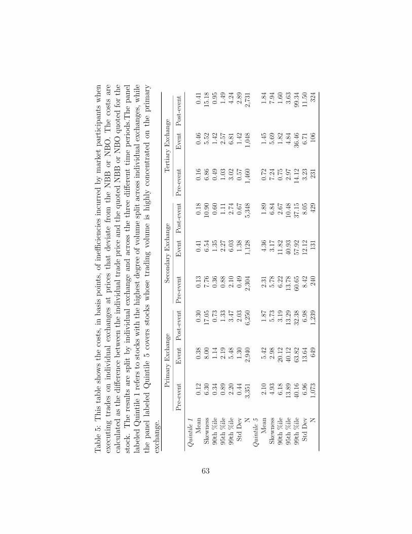
Tab
le5:
This
table
show
sth
eco
sts,
inbas
isp
oints
,of
ineffi
cien
cies
incu
rred
by
mar
ket
par
tici
pan
tsw
hen
exec
uti
ng
trad
eson
indiv
idual
exch
ange
sat
pri
ces
that
dev
iate
from
the
NB
Bor
NB
O.
The
cost
sar
eca
lcula
ted
asth
ediff
eren
ceb
etw
een
the
indiv
idual
trad
epri
cean
dth
equot
edN
BB
orN
BO
quot
edfo
rth
est
ock
.T
he
resu
lts
are
split
by
indiv
idual
exch
ange
and
acro
ssth
eth
ree
diff
eren
tti
me
per
iods.
The
pan
ella
bel
edQ
uin
tile
1re
fers
tost
ock
sw
ith
the
hig
hes
tdeg
ree
ofvo
lum
esp
lit
acro
ssin
div
idual
exch
ange
s,w
hile
the
pan
ella
bel
edQ
uin
tile
5co
vers
stock
sw
hos
etr
adin
gvo
lum
eis
hig
hly
conce
ntr
ated
onth
epri
mar
yex
chan
ge.
Pri
mar
yE
xch
ange
Sec
ond
ary
Exch
ange
Ter
tiar
yE
xch
ange
Pre
-eve
nt
Eve
nt
Pos
t-ev
ent
Pre
-eve
nt
Eve
nt
Pos
t-ev
ent
Pre
-eve
nt
Eve
nt
Pos
t-ev
ent
Qu
inti
le1
Mea
n0.
120.
380.
300.
130.
410.
180.
160.
460.
41S
kew
nes
s6.
308.
0017
.05
7.76
6.54
10.9
06.
865.
5215
.18
90th
%il
e0.
341.
140.
730.
361.
350.
600.
491.
420.
9595
th%
ile
0.89
2.19
1.33
0.88
2.27
1.11
1.03
2.57
1.49
99th
%il
e2.
205.
483.
472.
106.
032.
743.
026.
814.
24S
tdD
ev0.
441.
302.
030.
491.
380.
670.
571.
422.
89N
3,35
12,
940
6,25
02,
304
1,12
85,
348
1,46
01,
048
2,73
1Q
uin
tile
5M
ean
2.10
5.42
1.87
2.31
4.36
1.89
0.72
1.45
1.84
Ske
wn
ess
4.93
2.98
5.73
5.78
3.17
6.84
7.24
5.69
7.94
90th
%il
e6.
1820
.12
3.19
6.22
11.8
22.
670.
751.
821.
6095
th%
ile
13.8
940
.12
13.2
913
.78
40.9
310
.48
2.97
4.84
3.63
99th
%il
e40
.16
63.8
232
.38
60.6
557
.92
37.1
514
.12
36.4
699
.34
Std
Dev
6.96
13.6
46.
988.
4212
.12
8.05
3.23
6.71
11.5
0N
1,07
364
91,
239
240
131
429
231
106
324
63

In line with Aitken et al. (2017) who directly link improved market ef-
ficiency with increasing degrees of cross-market volume split, the difference
between the inefficiencies reported for Quintile 1 versus those documented
for Quintile 5 suggests that stocks with a higher degree of cross-listing are
traded more efficiently, when compared to their more concentrated counter-
parts. Taking the case of the primary exchange across the pre-event, event
and post-event periods, average costs associated with inefficiencies are about
17, 14 and 6 times higher for concentrated stocks. Moreover, these findings
also support the argumentation proposed in Bessembinder (2003), whereby
increased competition between individual exchanges results in decreases in
costs and general market conditions.
Secondly, comparing the incurred costs across the different time phases
of the event, increases in trade cost inefficiencies reported for trades exe-
cuted during the event minute, relative to those incurred during the pre-
event period, become evident. Looking at the mean reported values, it can
be observed that the stocks with the highest degree of cross-listing, exhibit
an increase from 0.12bp for the primary exchange, 0.13bp and 0.16bp for
the secondary and tertiary exchange, respectively, to 0.38bp, 0.41bp and
0.46bp, respectively. This translates into a more than 200% increase in cost
inefficiencies, across all exchanges. Increases of similar magnitude are also
documented when observing the figures in the second panel. Here, ineffi-
ciencies increase from pre-event levels of 2.10bp, 2.31bp and 0.72bp for the
primary, secondary and tertiary exchange to 5.42bp, 4.36bp and 1.45bp.
In order to further investigate differences in bid ask spread and trade
cost inefficiencies between cross-listed and concentrated securities in a mul-
tivariate setting, a series of OLS regressions are run. A dummy variable
(Cross-listed), which takes the value of one if a security belongs to the quin-
tile with the highest degree of cross-listing and zero when a security belongs
to the quintile with the highest degree of trading volume concentration on
a single exchange is included throughout all model specifications. Moreover,
64

Table 6: This table shows the coefficients of the OLS regressions aimed atinvestigating the differences in bid-ask spread, as well as in trade cost ineffi-ciencies calculated at a one-millisecond time interval between cross-listed se-curities and concentrated securities. All model specifications contain minutefixed effects, as well as firm level clustered standard errors. All coefficientsfor spread and cost metrics are expressed in basis points.t-statistics are re-ported in parentheses. *, **, *** denote significance at the p < .1, p < .05and p < .01 levels.
Primary Exchange Secondary Exchange Tertiary Exchange
Coeff t-stat Coeff t-stat Coeff t-stat
Panel Dependent Variable: Bid-Ask SpreadCross-listed -12.63*** -3.41 3.72 0.09 -72.26** -2.38Constant 17.07*** 5.80 23.53 1.06 76.43*** 2.98Minute FE Yes Yes YesN 20,460,000 20,460,000 20,460,000adj. R2 0.182 0.023 0.120
Panel Dependent Variable: Cost InefficienciesCross-listed -2.97** -2.13 -2.14** -2.05 -1.49 -1.11Constant 2.65** 2.33 2.20** 2.18 1.87 1.44Minute FE Yes Yes YesN 15,541 4,079 2,641adj. R2 0.012 0.008 0.011
65

all model specifications include minute fixed effects and clustered standard
errors at the security level. Table 6 reports on the coefficients for the six
model specifications. Referring to the first panel of Table 6, the negative
and statistically significant coefficients reported for the Cross-listed dummy
imply that on average, cross-listed securities exhibit a smaller bid-ask spread,
when looking at a security’s primary and tertiary exchange. Specifically, the
bid-ask spread is on average -12.63bp smaller for cross-listed securities when
compared to concentrated securities on the primary exchange, while the dif-
ference increases to -72.26bp, in the case of the tertiary exchange. The neg-
ative, statistically significant coefficient for the Cross-listed dummy variable
in the second panel of Table 6, suggests that incurred trade costs inefficien-
cies are indeed lower for cross-listed securities when referring to the cases of
the primary and secondary exchanges. Specifically, these incurred costs are
-2.97bp and -2.14bp smaller on the primary and secondary exchange, respec-
tively. In this respect these findings provide further evidence supporting the
idea that market fragmentation does not harm market quality.
However, the high degree of comparability in recorded cost inefficiencies
reported in Table 5 across individual exchanges and across each of the sep-
arate event periods suggests that such inefficiencies are uniformly observed
across all exchanges. It appears that there is no difference in trading activity
across the individual exchanges, supporting the idea of a unified US market
with multiple access points (individual exchanges).
In order to compare the individual cost inefficiency distributions, observed
on the individual exchanges, a series of two-sample Kolmogorov-Smirnov
tests for equality of distributions are performed. The null hypothesis states
that the two test samples belong to the same distribution. Specifically,
this nonparametric test calculates the distance of the first distribution to
its counterpart. The particular advantage of the selected approach is that
the Kolmogorov-Smirnov test takes into account both differences in location
and in the shape of the cumulative distribution functions corresponding to
66

the two compared samples.
Table 7: This table presents the results of the pairwise performed two-sampleKolmogorov-Smirnov tests for equality of distributions. The null hypothesisof the tests states that the two test samples belong to the same distribution.The test is performed pairwise across all three exchanges.
Primary vs. Secondary Secondary vs. Tertiary Primary vs. Tertiary
Benchmark Diff. P-Value Benchmark Diff. P-Value Benchmark Diff. P-ValuePrimary 0.01 0.71 Secondary 0.01 0.92 Primary 0.01 0.79
Secondary -0.02 0.19 Tertiary -0.03 0.12 Tertiary -0.04 0.01Combined K-S 0.02 0.37 Combined K-S 0.03 0.23 Combined K-S 0.04 0.02
Table 7 summarizes the results obtained when running two-sample Kolmogorov-
Smirnov tests pairwise for the three exchanges. Looking at the reported t-
values for the Combined K-S test, we fail to refute the null hypothesis of
the Combined K-S test in the case of the first two comparisons, primary vs.
secondary and secondary vs. tertiary exchange. Corroborating these results
with the summarized costs in Table 5 provides further evidence of the similar
pattern trade cost inefficiency throughout the individual exchanges.
Indeed, the Combined K-S t-value, reported when referring to the com-
parison of the primary vs. tertiary exchange, indicates the rejection of the
null hypothesis and therefore suggesting that in fact the cumulative dis-
tribution functions of the two trading cost inefficiencies distributions differ.
Specifically, the negative difference of -0.04 reported for the tertiary exchange
indicates that trading costs on the tertiary exchange are lower than those ob-
served on the primary exchange. Nevertheless, the low difference reported by
the test weaken the counter argument. Corroborating these results with the
summarized costs in Table 5 provides further evidence of the similar pattern
trade cost inefficiency throughout the individual exchanges.
Complementing these results, Table 8 summarizes the percent of per-
minute realized trading volume which has been traded in times during which
the exchange was deviating from the national best bid or national best of-
fer. Analogous to the case of the incurred cost inefficiencies, we observe
67

Tab
le8:
This
table
show
sth
ep
erce
nt
ofp
er-m
inute
trad
ing
volu
me,
that
occ
urs
onth
ein
div
idual
exch
ange
s,in
tim
esduri
ng
whic
hth
eex
chan
geis
not
quot
ing
eith
erth
enat
ional
bes
tbid
ornat
ional
bes
tas
k.
The
resu
lts
are
split
by
indiv
idual
exch
ange
and
acro
ssth
eth
ree
diff
eren
tti
me
per
iods.
The
pan
ella
bel
edQ
uin
tile
1re
fers
tost
ock
sw
ith
the
hig
hes
tdeg
ree
ofvo
lum
esp
lit
acro
ssin
div
idual
exch
ange
s,w
hile
the
pan
ella
bel
edQ
uin
tile
5co
vers
stock
sw
hos
etr
adin
gvo
lum
eis
hig
hly
conce
ntr
ated
onth
epri
mar
yex
chan
ge.
Pri
mar
yE
xch
ange
Sec
ond
ary
Exch
ange
Ter
tiar
yE
xch
ange
Pre
-eve
nt
Eve
nt
Pos
t-ev
ent
Pre
-eve
nt
Eve
nt
Pos
t-ev
ent
Pre
-eve
nt
Eve
nt
Pos
t-ev
ent
Qu
inti
le1
Mea
n14
.26%
30.0
2%25
.66%
12.3
9%29
.17%
20.0
0%15
.10%
28.7
0%22
.68%
Med
ian
12.2
5%32
.54%
23.1
5%7.
25%
32.3
1%21
.14%
6.92
%30
.52%
19.4
7%90
th%
ile
28.5
2%43
.51%
52.0
2%35
.24%
46.0
9%36
.59%
45.1
8%45
.26%
52.3
4%95
th%
ile
38.9
1%45
.42%
67.1
6%48
.77%
59.3
1%40
.86%
52.5
6%45
.32%
54.8
6%99
th%
ile
72.2
1%45
.42%
100.
00%
59.9
3%59
.31%
100.
00%
66.6
8%45
.32%
100.
00%
Std
Dev
14.4
7%12
.12%
20.4
0%15
.01%
15.3
0%15
.86%
17.8
7%10
.25%
21.1
8%Q
uin
tile
5M
ean
33.1
4%43
.09%
34.7
5%23
.53%
37.5
3%35
.94%
14.3
9%20
.66%
24.5
5%M
edia
n18
.45%
27.3
9%28
.01%
0.00
%14
.81%
25.0
7%0.
00%
16.0
0%17
.12%
90th
%il
e10
0.00
%86
.72%
97.4
1%10
0.00
%89
.11%
100.
00%
59.3
8%33
.54%
84.8
8%95
th%
ile
100.
00%
100.
00%
100.
00%
100.
00%
100.
00%
100.
00%
100.
00%
100.
00%
100.
00%
99th
%il
e10
0.00
%10
0.00
%10
0.00
%10
0.00
%10
0.00
%10
0.00
%10
0.00
%10
0.00
%10
0.00
%S
tdD
ev34
.92%
29.5
8%31
.53%
37.1
2%37
.16%
37.9
3%29
.41%
26.0
4%29
.65%
68

evident similarities when comparing the mean values reported for the indi-
vidual exchanges across the pre-event and event periods for stocks included
in Quintile 1. Specifically, 14.26% of the trading volume occurring on the
primary exchange during the pre-event period happens when the exchange
quotes prices which are either below or above the national best bid or na-
tional best ask respectively, versus 12.39% and 15.10% in the case of the
secondary and tertiary exchanges. These figures increase to 30.02%, 29.17%
and 28.70% for the primary, secondary and tertiary exchanges respectively
during the event-minute. Nevertheless, similarities in reported volume pat-
terns disappear when turning to the figures reported for Quintile 5. The
primary exchange, which referring back to the figures in Table 4, handles on
average 78.33% of the total volume reported by an individual stock, reports
that 33.14% of the trading volume took place outside the national best bid
or national best ask during the pre-event period, 43.09% during the event
minute and 34.75% during the post-event period. The figures for the sec-
ondary and tertiary exchange are indeed throughout all time periods lower
when benchmarked against the primary exchange. This comes in strong con-
trast to the developments in the stocks with the highest volume split across
individual exchanges, suggesting that decreased inter-exchange competition
could in fact cause market participants to bear increased inefficiencies.
Overall, the presented results confirm the findings presented in extant
literature covering cross-listed securities, whereby supporting and providing
alternative evidence that stocks with an increased split in trading volume
across multiple regional exchanges offer better market conditions. Both in-
curred cost inefficiencies and trading volume outside the national best bid
and ask are substantially higher for stocks whose trading volume is concen-
trated solely on the primary exchange. Nevertheless, when strictly looking
at liquidity, as measured by the quoted bid-ask spread, the primary exchange
dominates its peers and remains the best trading venue.
69

5. Conclusion
This paper analyzes general market conditions and in particular liquidity
and trading activity in times of extreme events such as the one on Decem-
ber 19, 2018, when at 14:00, the Federal Open Market Committee (FOMC),
through its regular communication channel, published a press release an-
nouncing a 25bp interest rate increase and expressed concerns about po-
tentially deteriorating macro-economic conditions. The event triggered an
immediate decline in major US indexes, whereby 71 cross-listed Nasdaq100
index constituents experienced a three sigma negative price movement.
Liquidity conditions deteriorate in the event-period, the minute immedi-
ately following up the Fed’s announcement, with threefold reported increases
in bid-ask spread across all individual exchanges. Trading volume, as well
as the number of executed trades increase when compared to the 5-minute
pre-event interval. Despite increasing bid-ask spreads, the primary listing
exchange remains superior in terms of liquidity across all time event periods.
Benchmarked against the secondary and tertiary exchanges, the primary ex-
change is quoting 81.96% and 81.15% percent of the time bid and ask prices
prices which are equally best or superior.
Furthermore, the paper documents an increase in trade cost inefficiencies,
measured as trades executed below the national best bid or above national
best ask, across all three individual exchanges, in both cross-listed and single
exchange concentrated stocks, in the period covering the fist minute after the
Fed’s decision to increase interest rates when compared to pre-event levels.
Nevertheless, the analysis reports similarities in trade cost inefficiencies
and volume patterns when looking at stocks with an increased volume split
across individual exchanges, while the opposite is observed in the case for
stocks who mainly trade on one exchange.
70

References
Admati, A. R. and Pfleiderer, P. (1988). A theory of intraday patterns:
Volume and price variability. he Review of Financial Studies, 1(1):3–40.
Aitken, M., Chen, H., and SeanFoley (2017). The impact of fragmentation,
exchange fees and liquidity provision on market quality. Journal of Em-
pirical Finance, 41:120–160.
Battalio, R. H. (1997). Third market broker-dealers: Cost competitors or
cream skimmers? The Journal of Finance, 52(1):341–352.
Bessembinder, H. (2003). Quote-based competition and trade executioncosts
in NYSE-listed stocks. Journal of Financial Economics, 70:85–422.
Bjørnland, H. C. and Leitemo, K. (2009). Identifying the interdependence
between US monetary policy and the stock market. Journal of Monetary
Economics, 56(2):275–282.
Bolton, P., Santos, T., and Scheinkman, J. A. (2016). Cream-skimming in
financial markets. The Journal of Finance, 71(2):709–736.
Boubaker, S., Gounopoulos, D., Nguyen, D. K., and Paltalidis, N. (2018).
Reprint of: Assessing the effects of unconventional monetary policy and
low interest rates on pension fund risk incentives. Journal of Banking &
Finance, 92:340–357.
Brogaard, J., Carrionb, A., Moyaert, T., Riordan, R., Shkilko, A., and
Sokolov, K. (2018). High frequency trading and extreme price movements.
Journal of Financial Economics, 128(2):253–265.
Brogaard, J., Hendershott, T., and Riordan, R. (2014). High-frequency trad-
ing and price discovery. Review of Financial Studies, 27(8):2267–2306.
71

Campbell, J. Y. (1987). Stock returns and the term structure. Journal of
Financial Economics, 18(2):373–399.
Carrion, A. (2013). Very fast money: High-frequency trading on the NAS-
DAQ. Journal of Financial Markets, 16:680–711.
Chen, N. (1991). Financial investment opportunities and the macroeconomy.
The Journal of Finance, 46(2):529–554.
Chen, N., Roll, R., and Ross, S. A. (1986). Economic forces and the stock
market. The Journal of Business, 59(3):383–403.
Chen, S. (2009). Predicting the bear stock market: Macroeconomic variables
as leading indicators. Journal of Banking & Finance, 33(2):211–223.
Chordia, T., Roll, R., and Subrahmanyam, A. (2002). Market liquidity and
trading activity. The Journal of Finance, 56(2):501–530.
Chordia, T., Roll, R., and Subrahmanyam, A. (2011). Recent trends in
trading activity and market quality. Journal of Financial Economics,
101(2):243–263.
Christiansen, C. and Ranaldo, A. (2007). Realized bond-stock correlation:
Macroeconomic announdement effects. The Journal of Futures Markets,
27(5):439–469.
Chulia, H., Martens, M., and van Dijk, D. (2010). Asymmetric effects of
federal funds target rate changes on S&P100 stock returns, volatilities and
correlations. Journal of Banking & Finance, 34(4):834–839.
Easley, D., Kiefer, N. M., and O’Hara, M. (1996). Cream-skimming or profit-
sharing? the curious role of purchased order flow. The Journal of Finance,
51(3):811–833.
72

Elyasiani, E. and Mansur, I. (1998). Sensitivity of the bank stock returns
distribution to changes in the level and volatility of interest rate: A garch-
m model. Journal of Banking & Finance, 22(5):535–563.
Erenburg, G. and Lasser, D. (2009). Electronic limit order book and or-
der submission choice around macroeconomic news. Review of Financial
Economics, 18(4):172–182.
Eun, C. S. and Sabherwal, S. (2003). Cross-border listings and price discov-
ery: Evidence from U.S.-listed Canadian stocks. The Journal of Finance,
58(2):549–575.
Fama, E. F. (1981). Stock returns, real activity, inflation, and money. The
American Economic Review, 71(4):545–565.
Flannery, M. J. and James, C. M. (1984). The effect of interest rate changes
on the common stock returns of financial institutions. Journal of Finance,
39(4):1141–1153.
Foucault, T., Hombert, J., and Rosu, I. (2015). News trading and speed.
The Journal of Finance, 71(1).
Hasbrouck, J. and Schwartz, R. A. (1988). Liquidity and execution costs in
equity markets. Journal of Portfolio Management, 14:10–16.
Holden, C. W. and Jacobsen, S. (2014). Liquidity measurement problems in
fast, competitive markets: Expensive and cheap solutions. The Journal of
Finance, 69(4):1747–1785.
Kontonikas, A., MacDonald, R., and Saggub, A. (2013). Stock market reac-
tion to fed funds rate surprises: State dependence and the financial crisis.
Journal of Banking & Finance, 37(11):4025–4037.
Lee, C. M. and Swaminathan, B. (2000). Price momentum and trading
volume. The Journal of Finance, 55(5):2017–2069.
73

Menkveld, A. J. (2013). High frequency trading and the new market makers.
Journal of Financial Markets, 16(4):712–740.
Nagel, S. (2012). Evaporating liquidity. The Review of Financial Studies,
25(7):2005–2039.
O’Hara, M. and Ye, M. (2011). Is market fragmentation harming market
quality? Journal of Financial Economics, pages 459–474.
Rif, A. and Utz, S. (2019). Short-term stock price reversals after extreme
events.
Scholtus, M., van Dijka, D., and Frijns, B. (2014). Speed, algorithmic trading,
and market quality around macroeconomic news announcements. Journal
of Banking & Finance, 38:89–105.
SEC (2005). Regulation NMS, release no. 34-51808; file no. s7-10-04 edition.
SEC (2015). Memorandum: Rule 611 of Regulation NMS. Division of Trading
and Markets.
Stoll, H. R. (2001). Market fragmentation. Financial Analysts Journal,
57(4):16–20.
Upson, J. and VanNess, R. A. (2017). Multiple markets, algorithmic trading,
and market liquidity. Journal of Financial Markets, 32:49–68.
74

Appendix
Table 9: Complete description of abnormal quote conditions which havebeen excluded in line with the data cleaning process described in Holden andJacobsen (2014), as well as the additional equity symbol suffixes for whichobservations from the daily trades dataset have not been included.
Quote Condition Description
A This condition indicates that the current offer is in ‘Slow’ quote mode.While in this mode, autoexecution is not eligible on the Offer side andcan be traded through pursuant to anticipated Regulation NMS require-ments
B This condition indicates that the current bid is in ‘Slow’ quote mode.While in this mode, autoexecution is not eligible on the Bid side andcan be traded through pursuant to anticipated Regulation NMS require-ments.
H This condition indicates that the quote is a ‘Slow’ quote on both the Bidand Offer sides. While in this mode, auto-execution is not eligible onthe Bid and Offer sides, and either or both sides can be traded throughpursuant to anticipated Regulation NMS requirements.
O This condition can be disseminated to indicate that this quote was theopening quote for a security for that Participant.
R This condition is used for the majority of quotes to indicate a normaltrading environment. It is also used by the FINRA Market Makers inplace of Quote Condition ‘O’ to indicate the first quote of the day fora particular security. The condition may also be used when a MarketMaker re-opens a security during the day.
W This quote condition is used to indicate that the quote is a Slow Quoteon both the Bid and Offer sides due to a Set Slow List that includesHigh Price securities. While in this mode, auto-execution is not eligible,the quote is then considered Slow on the Bid and Offer sides and eitheror both sides can be traded through, as per Regulation NMS.
Equity Suffix Description
K Non-Voting Shares
L Miscellaneous situations such as certificates of participation, preferredparticipation, and stubs
V Denotes a transaction in a security authorized for issuance, but not yetissued. All “when issued” transactions are on an “if” basis, to be settledif and when the actual security is issued.
Z Miscellaneous situations such as certificates of preferred when issued
75

Table 10: This table shows the percentage of trade volume per minute inter-val, which given the rules specified under SEC NMS Regulation - Rule 611would classify as trade-through volume. Specifically, Inter-market SweepOrders have been dropped from the dataset. Additionally, a the one-secondtime window rule has also been applied, prohibiting the classification of agiven trade as a trade-through if the exchange at hand had quoted either atthe national best bid or national best ask within a one-second time window.
Primary ExchangeInterval Mean Skewness 95th %ile 99th %ile Std Dev Nr. Trades
t-5 1.43% 7.53 5.11% 35.31% 7.42% 802t-4 0.55% 6.54 2.68% 22.40% 2.80% 990t-3 0.35% 12.33 0.00% 11.75% 3.51% 800t-2 0.71% 6.55 4.15% 24.46% 3.70% 618t-1 1.22% 9.47 1.20% 30.58% 8.58% 1509
t 0.14% 13.84 0.00% 2.90% 1.26% 3623t+1 0.63% 13.64 0.00% 23.04% 5.04% 1578t+2 0.04% 9.70 0.17% 0.17% 0.24% 1404t+3 0.30% 10.23 0.00% 14.71% 2.67% 1263t+4 0.17% 10.11 0.00% 4.10% 1.22% 2059t+5 0.33% 9.93 1.37% 13.21% 2.11% 1392
Secondary ExchangeInterval Mean Skewness 95th %ile 99th %ile Std Dev Nr. Trades
t-5 0.94% 7.47 6.95% 37.66% 4.33% 333t-4 0.25% 6.48 0.00% 11.10% 1.64% 405t-3 0.22% 21.28 0.00% 0.00% 4.68% 456t-2 0.22% 5.94 0.00% 8.58% 1.37% 421t-1 0.99% 13.93 3.11% 18.38% 5.05% 579
t 1.26% 4.22 3.50% 18.85% 2.82% 1035t+1 0.95% 4.28 3.50% 15.52% 2.83% 584t+2 0.20% 9.23 0.00% 13.32% 1.82% 624t+3 0.31% 9.33 0.49% 22.64% 2.36% 730t+4 0.19% 12.67 0.00% 1.06% 1.92% 1350t+5 0.25% 5.85 0.00% 8.94% 1.46% 781
Tertiary ExchangeInterval Mean Skewness 95th %ile 99th %ile Std Dev Nr. Trades
t-5 0.26% 9.61 0.00% 24.99% 2.55% 286t-4 0.00% . 0.00% 0.00% 0.00% 349t-3 0.21% 12.90 0.15% 0.15% 2.56% 339t-2 0.00% . 0.00% 0.00% 0.00% 275t-1 1.43% 6.11 3.91% 33.31% 5.51% 471
t 1.97% 7.51 7.86% 87.15% 9.90% 877t+1 1.18% 11.34 10.43% 13.69% 5.65% 537t+2 2.12% 6.87 1.04% 49.97% 11.56% 510t+3 1.15% 7.77 0.00% 16.70% 6.52% 369t+4 0.87% 9.22 5.23% 5.23% 4.01% 850t+5 0.86% 12.36 4.67% 6.02% 6.69% 605
76
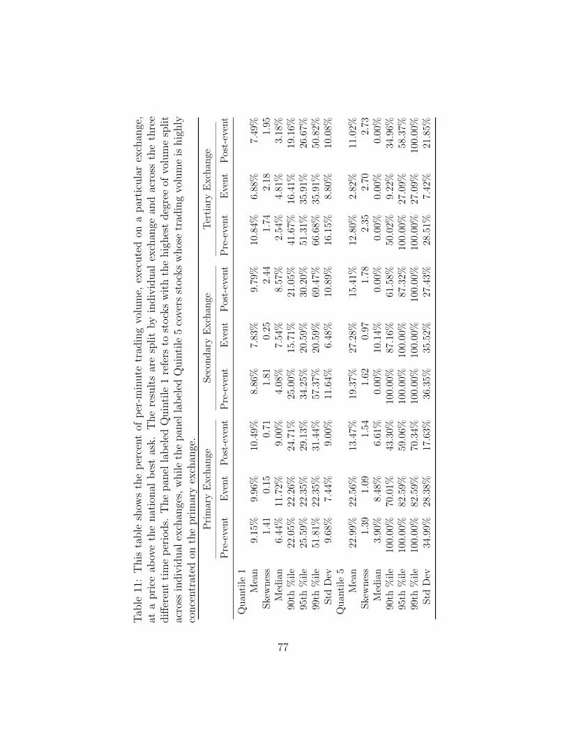
Tab
le11
:T
his
table
show
sth
ep
erce
nt
ofp
er-m
inute
trad
ing
volu
me,
exec
ute
don
apar
ticu
lar
exch
ange
,at
apri
ceab
ove
the
nat
ional
bes
tas
k.
The
resu
lts
are
split
by
indiv
idual
exch
ange
and
acro
ssth
eth
ree
diff
eren
tti
me
per
iods.
The
pan
ella
bel
edQ
uin
tile
1re
fers
tost
ock
sw
ith
the
hig
hes
tdeg
ree
ofvo
lum
esp
lit
acro
ssin
div
idual
exch
ange
s,w
hile
the
pan
ella
bel
edQ
uin
tile
5co
vers
stock
sw
hos
etr
adin
gvo
lum
eis
hig
hly
conce
ntr
ated
onth
epri
mar
yex
chan
ge.
Pri
mar
yE
xch
ange
Sec
ond
ary
Exch
ange
Ter
tiar
yE
xch
ange
Pre
-eve
nt
Eve
nt
Pos
t-ev
ent
Pre
-eve
nt
Eve
nt
Pos
t-ev
ent
Pre
-eve
nt
Eve
nt
Pos
t-ev
ent
Qu
anti
le1
Mea
n9.
15%
9.96
%10
.49%
8.86
%7.
83%
9.79
%10
.84%
6.88
%7.
49%
Ske
wn
ess
1.41
0.15
0.71
1.81
0.25
2.44
1.74
2.18
1.95
Med
ian
6.44
%11
.72%
9.00
%4.
08%
7.54
%8.
57%
2.54
%4.
81%
3.18
%90
th%
ile
22.0
5%22
.26%
24.7
1%25
.00%
15.7
1%21
.05%
41.6
7%16
.41%
19.1
6%95
th%
ile
25.5
9%22
.35%
29.1
3%34
.25%
20.5
9%30
.20%
51.3
1%35
.91%
26.6
7%99
th%
ile
51.8
1%22
.35%
31.4
4%57
.37%
20.5
9%69
.47%
66.6
8%35
.91%
50.8
2%S
tdD
ev9.
68%
7.44
%9.
00%
11.6
4%6.
48%
10.8
9%16
.15%
8.80
%10
.08%
Qu
anti
le5
Mea
n22
.99%
22.5
6%13
.47%
19.3
7%27
.28%
15.4
1%12
.80%
2.82
%11
.02%
Ske
wn
ess
1.39
1.09
1.54
1.62
0.97
1.78
2.35
2.70
2.73
Med
ian
3.90
%8.
48%
6.61
%0.
00%
10.1
4%0.
00%
0.00
%0.
00%
0.00
%90
th%
ile
100.
00%
70.0
1%43
.30%
100.
00%
87.1
6%61
.58%
50.0
2%9.
22%
34.9
6%95
th%
ile
100.
00%
82.5
9%59
.06%
100.
00%
100.
00%
87.3
2%10
0.00
%27
.09%
58.3
7%99
th%
ile
100.
00%
82.5
9%70
.34%
100.
00%
100.
00%
100.
00%
100.
00%
27.0
9%10
0.00
%S
tdD
ev34
.99%
28.3
8%17
.63%
36.3
5%35
.52%
27.4
3%28
.51%
7.42
%21
.85%
77

Tab
le12
:T
his
table
show
sth
ep
erce
nt
ofp
er-m
inute
trad
ing
volu
me,
exec
ute
don
apar
ticu
lar
exch
ange
,at
apri
ceb
elow
the
nat
ional
bes
tbid
.T
he
resu
lts
are
split
by
indiv
idual
exch
ange
and
acro
ssth
eth
ree
diff
eren
tti
me
per
iods.
The
pan
ella
bel
edQ
uin
tile
1re
fers
tost
ock
sw
ith
the
hig
hes
tdeg
ree
ofvo
lum
esp
lit
acro
ssin
div
idual
exch
ange
s,w
hile
the
pan
ella
bel
edQ
uin
tile
5co
vers
stock
sw
hos
etr
adin
gvo
lum
eis
hig
hly
conce
ntr
ated
onth
epri
mar
yex
chan
ge.
Pri
mar
yE
xch
ange
Sec
ond
ary
Exch
ange
Ter
tiar
yE
xch
ange
Pre
-eve
nt
Eve
nt
Pos
t-ev
ent
Pre
-eve
nt
Eve
nt
Pos
t-ev
ent
Pre
-eve
nt
Eve
nt
Pos
t-ev
ent
Qu
anti
le1
Mea
n5.
24%
20.1
1%15
.55%
3.53
%21
.34%
10.2
1%4.
25%
21.8
1%15
.22%
Ske
wn
ess
2.37
0.01
2.89
3.40
1.05
0.82
2.07
-0.3
62.
28M
edia
n2.
71%
19.5
5%11
.95%
0.00
%19
.44%
9.25
%0.
00%
23.2
1%8.
53%
90th
%il
e17
.01%
31.5
6%31
.07%
11.4
7%38
.23%
22.6
5%17
.69%
32.7
6%36
.08%
95th
%il
e25
.35%
39.7
0%49
.42%
23.0
0%59
.31%
30.5
3%25
.01%
32.8
3%47
.34%
99th
%il
e36
.80%
39.7
0%10
0.00
%46
.12%
59.3
1%39
.16%
33.3
6%32
.83%
100.
00%
Std
Dev
8.36
%9.
62%
18.2
2%7.
88%
13.6
3%9.
54%
8.17
%8.
51%
19.3
0%Q
uan
tile
5M
ean
11.0
4%23
.85%
22.2
5%4.
94%
10.2
5%23
.05%
1.59
%17
.84%
13.5
3%S
kew
nes
s2.
010.
071.
534.
502.
231.
296.
432.
182.
27M
edia
n0.
00%
21.0
4%8.
06%
0.00
%0.
00%
0.00
%0.
00%
13.8
7%0.
00%
90th
%il
e37
.36%
45.0
6%94
.81%
19.7
5%33
.27%
100.
00%
0.50
%33
.54%
34.8
3%95
th%
ile
54.8
6%45
.33%
100.
00%
32.7
2%69
.28%
100.
00%
4.86
%10
0.00
%84
.96%
99th
%il
e83
.40%
45.3
3%10
0.00
%10
0.00
%69
.28%
100.
00%
59.3
8%10
0.00
%10
0.00
%S
tdD
ev17
.72%
13.0
4%31
.43%
15.0
7%18
.44%
35.3
4%8.
50%
26.5
0%25
.45%
78
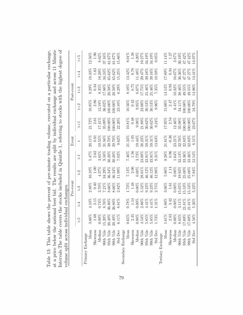
Tab
le13
:T
his
table
show
sth
ep
erce
nt
ofp
er-m
inute
trad
ing
volu
me,
exec
ute
don
apar
ticu
lar
exch
ange
,at
apri
ceb
elow
the
nat
ional
bes
tbid
.T
he
resu
lts
are
split
by
indiv
idual
exch
ange
and
acro
ss11
Min
ute
Inte
rval
s.T
he
table
cove
rsth
est
ock
sin
cluded
inQ
uin
tile
1,re
ferr
ing
tost
ock
sw
ith
the
hig
hes
tdeg
ree
ofvo
lum
esp
lit
acro
ssin
div
idual
exch
ange
s.
Pre
-eve
nt
Eve
nt
Pos
t-ev
ent
t-5
t-4
t-3
t-2
t-1
tt+
1t+
2t+
3t+
4t+
5
Pri
mar
yE
xch
ange
Mea
n3.
66%
4.10
%2.
88%
10.1
0%5.
47%
20.1
1%21
.72%
16.8
5%8.
29%
18.3
3%12
.56%
Ske
wnes
s1.
683.
150.
401.
002.
620.
012.
612.
860.
341.
631.
96M
edia
n0.
00%
0.74
%3.
70%
4.37
%3.
85%
19.5
5%17
.41%
12.1
9%8.
35%
18.2
9%8.
02%
90th
%ile
15.2
0%8.
76%
7.21
%34
.29%
9.50
%31
.56%
35.0
9%36
.02%
17.8
6%34
.24%
37.1
6%95
th%
ile
20.4
9%36
.80%
8.66
%36
.34%
30.2
0%39
.70%
100.
00%
100.
00%
20.5
0%65
.62%
61.6
7%99
th%
ile
20.4
9%36
.80%
8.66
%36
.34%
30.2
0%39
.70%
100.
00%
100.
00%
20.5
0%65
.62%
61.6
7%Std
Dev
6.11
%8.
81%
2.82
%11
.99%
7.03
%9.
62%
22.2
0%23
.10%
6.29
%15
.25%
15.8
6%Sec
ondar
yE
xch
ange
Mea
n0.
65%
0.78
%1.
73%
7.13
%7.
46%
21.3
4%10
.81%
10.5
6%8.
18%
13.4
2%8.
01%
Ske
wnes
s2.
351.
541.
482.
001.
561.
050.
480.
420.
750.
781.
38M
edia
n0.
00%
0.00
%0.
00%
0.00
%3.
73%
19.4
4%9.
98%
9.95
%6.
07%
11.4
8%8.
20%
90th
%ile
4.54
%2.
86%
5.52
%28
.01%
23.0
0%38
.23%
21.8
9%23
.00%
17.7
5%29
.47%
19.2
7%95
th%
ile
5.85
%4.
41%
9.23
%46
.12%
33.9
1%59
.31%
30.6
2%30
.53%
25.4
6%39
.16%
34.1
9%99
th%
ile
5.85
%4.
41%
9.23
%46
.12%
33.9
1%59
.31%
30.6
2%30
.53%
25.4
6%39
.16%
34.1
9%Std
Dev
1.73
%1.
31%
2.75
%12
.98%
9.31
%13
.63%
9.24
%9.
96%
7.35
%10
.59%
9.05
%T
erti
ary
Exch
ange
Mea
n1.
61%
1.80
%3.
06%
5.86
%9.
28%
21.8
1%17
.95%
15.0
0%14
.14%
17.8
9%11
.14%
Ske
wnes
s2.
833.
421.
611.
140.
96-0
.36
2.54
2.47
0.93
0.34
1.27
Med
ian
0.00
%0.
00%
0.00
%0.
00%
1.64
%23
.21%
12.4
6%6.
41%
10.3
2%16
.67%
3.87
%90
th%
ile
8.05
%3.
11%
15.0
5%19
.92%
32.1
3%32
.76%
35.9
8%34
.11%
38.4
6%36
.36%
36.1
9%95
th%
ile
17.6
9%21
.81%
15.5
3%25
.00%
33.3
6%32
.83%
100.
00%
100.
00%
49.5
5%47
.27%
47.4
2%99
th%
ile
17.6
9%21
.81%
15.5
3%25
.00%
33.3
6%32
.83%
100.
00%
100.
00%
49.5
5%47
.27%
47.4
2%Std
Dev
4.58
%5.
26%
5.22
%7.
94%
12.5
4%8.
51%
23.6
7%24
.79%
14.9
6%14
.41%
14.9
7%
79

Tab
le14
:T
his
table
show
sth
ep
erce
nt
ofp
er-m
inute
trad
ing
volu
me,
exec
ute
don
apar
ticu
lar
exch
ange
,at
apri
ceb
elow
the
nat
ional
bes
tbid
.T
he
resu
lts
are
split
by
indiv
idual
exch
ange
and
acro
ss11
Min
ute
Inte
rval
s.T
he
table
cove
rsth
est
ock
sin
cluded
inQ
uin
tile
5,re
ferr
ing
tost
ock
sw
ith
the
low
est
deg
ree
ofvo
lum
esp
lit
acro
ssin
div
idual
exch
ange
s.P
re-e
vent
Eve
nt
Pos
t-ev
ent
t-5
t-4
t-3
t-2
t-1
tt+
1t+
2t+
3t+
4t+
5
Pri
mar
yE
xch
ange
Mea
n2.
30%
6.49
%12
.96%
17.0
0%16
.46%
23.8
5%34
.48%
31.9
0%19
.29%
21.8
5%4.
53%
Ske
wnes
s1.
202.
351.
861.
600.
270.
070.
840.
911.
810.
891.
97M
edia
n0.
00%
0.00
%8.
31%
5.74
%12
.46%
21.0
4%23
.33%
12.2
9%2.
59%
18.5
8%0.
00%
90th
%ile
8.34
%28
.77%
54.8
6%56
.07%
37.8
6%45
.06%
100.
00%
100.
00%
100.
00%
55.8
0%25
.19%
95th
%ile
11.1
2%52
.24%
64.9
4%83
.40%
38.0
6%45
.33%
100.
00%
100.
00%
100.
00%
68.5
3%31
.13%
99th
%ile
11.1
2%52
.24%
64.9
4%83
.40%
38.0
6%45
.33%
100.
00%
100.
00%
100.
00%
68.5
3%31
.13%
Std
Dev
3.89
%14
.34%
19.2
8%23
.94%
15.4
6%13
.04%
36.6
3%37
.92%
33.3
0%20
.64%
9.68
%Sec
ondar
yE
xch
ange
Mea
n0.
00%
0.19
%5.
87%
6.84
%10
.79%
10.2
5%38
.97%
28.8
2%23
.75%
27.9
4%0.
50%
Ske
wnes
s.
3.18
1.81
1.33
3.01
2.23
0.60
0.96
1.07
0.95
3.33
Med
ian
0.00
%0.
00%
0.00
%0.
00%
0.00
%0.
00%
30.4
8%2.
04%
0.00
%10
.10%
0.00
%90
th%
ile
0.00
%0.
00%
32.7
2%28
.97%
19.9
8%33
.27%
100.
00%
100.
00%
66.5
6%86
.99%
0.00
%95
th%
ile
0.00
%2.
53%
37.7
3%33
.34%
100.
00%
69.2
8%10
0.00
%10
0.00
%10
0.00
%10
0.00
%6.
96%
99th
%ile
0.00
%2.
53%
37.7
3%33
.34%
100.
00%
69.2
8%10
0.00
%10
0.00
%10
0.00
%10
0.00
%6.
96%
Std
Dev
0.00
%0.
67%
13.1
7%12
.18%
25.5
2%18
.44%
38.5
9%42
.11%
33.2
8%34
.83%
1.79
%T
erti
ary
Exch
ange
Mea
n0.
00%
6.60
%0.
00%
0.30
%1.
32%
17.8
4%6.
62%
37.0
0%3.
69%
16.8
4%7.
17%
Ske
wnes
s.
2.47
.2.
272.
292.
181.
110.
571.
941.
872.
43M
edia
n0.
00%
0.00
%0.
00%
0.00
%0.
00%
13.8
7%0.
00%
14.0
0%0.
00%
11.1
5%0.
00%
90th
%ile
0.00
%59
.38%
0.00
%2.
44%
4.86
%33
.54%
26.0
2%10
0.00
%14
.96%
34.8
3%19
.39%
95th
%ile
0.00
%59
.38%
0.00
%2.
44%
10.5
3%10
0.00
%27
.55%
100.
00%
25.6
9%84
.96%
59.5
3%99
th%
ile
0.00
%59
.38%
0.00
%2.
44%
10.5
3%10
0.00
%27
.55%
100.
00%
25.6
9%84
.96%
59.5
3%Std
Dev
0.00
%18
.66%
0.00
%0.
81%
3.08
%26
.50%
10.9
7%42
.48%
8.16
%22
.95%
17.4
6%
80
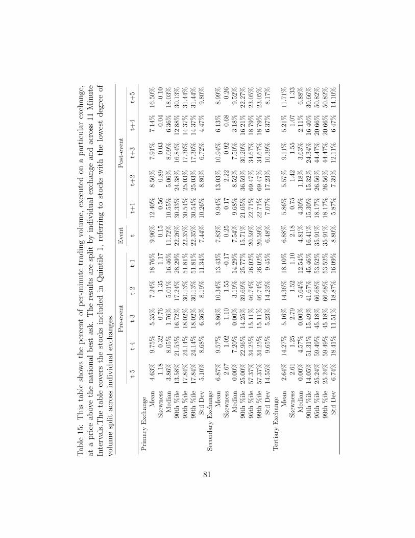
Tab
le15
:T
his
table
show
sth
ep
erce
nt
ofp
er-m
inute
trad
ing
volu
me,
exec
ute
don
apar
ticu
lar
exch
ange
,at
apri
ceab
ove
the
nat
ional
bes
tas
k.
The
resu
lts
are
split
by
indiv
idual
exch
ange
and
acro
ss11
Min
ute
Inte
rval
s.T
he
table
cove
rsth
est
ock
sin
cluded
inQ
uin
tile
1,re
ferr
ing
tost
ock
sw
ith
the
low
est
deg
ree
ofvo
lum
esp
lit
acro
ssin
div
idual
exch
ange
s.
Pre
-eve
nt
Eve
nt
Pos
t-ev
ent
t-5
t-4
t-3
t-2
t-1
tt+
1t+
2t+
3t+
4t+
5
Pri
mar
yE
xch
ange
Mea
n4.
63%
9.75
%5.
35%
7.24
%18
.76%
9.96
%12
.40%
8.50
%7.
91%
7.14
%16
.50%
Ske
wn
ess
1.18
0.32
0.76
1.35
1.17
0.15
0.56
0.89
0.03
-0.0
4-0
.10
Med
ian
3.86
%8.
05%
1.76
%5.
01%
16.4
6%11
.72%
10.5
5%5.
06%
8.09
%6.
36%
18.0
3%90
th%
ile
13.5
8%21
.53%
16.7
2%17
.24%
28.2
9%22
.26%
30.3
3%24
.38%
16.8
4%12
.88%
30.1
3%95
th%
ile
17.8
4%24
.14%
18.0
2%30
.13%
51.8
1%22
.35%
30.5
4%25
.03%
17.3
6%14
.37%
31.4
4%99
th%
ile
17.8
4%24
.14%
18.0
2%30
.13%
51.8
1%22
.35%
30.5
4%25
.03%
17.3
6%14
.37%
31.4
4%S
tdD
ev5.
10%
8.68
%6.
36%
8.19
%11
.34%
7.44
%10
.26%
8.80
%6.
72%
4.47
%9.
80%
Sec
ond
ary
Exch
ange
Mea
n6.
87%
9.57
%3.
86%
10.3
4%13
.43%
7.83
%9.
94%
13.0
3%10
.94%
6.13
%8.
99%
Ske
wn
ess
2.67
1.02
1.10
1.55
-0.1
70.
250.
172.
220.
920.
680.
26M
edia
n0.
00%
7.20
%0.
00%
3.19
%14
.29%
7.54
%9.
68%
8.52
%7.
50%
3.18
%9.
52%
90th
%il
e25
.00%
22.9
6%14
.25%
39.6
9%25
.77%
15.7
1%21
.05%
36.5
9%30
.20%
16.2
1%22
.27%
95th
%il
e57
.37%
34.2
5%15
.11%
46.7
4%26
.02%
20.5
9%22
.71%
69.4
7%34
.67%
18.7
9%23
.05%
99th
%il
e57
.37%
34.2
5%15
.11%
46.7
4%26
.02%
20.5
9%22
.71%
69.4
7%34
.67%
18.7
9%23
.05%
Std
Dev
14.5
5%9.
65%
5.23
%14
.23%
9.45
%6.
48%
7.07
%17
.23%
10.3
9%6.
37%
8.17
%T
erti
ary
Exch
ange
Mea
n2.
64%
14.2
7%5.
16%
14.3
6%18
.10%
6.88
%5.
86%
5.57
%9.
11%
5.21
%11
.71%
Ske
wn
ess
2.61
1.25
2.79
1.52
1.10
2.18
0.75
1.42
1.55
1.07
1.33
Med
ian
0.00
%4.
57%
0.00
%5.
64%
12.5
4%4.
81%
4.30
%1.
18%
3.63
%2.
11%
6.88
%90
th%
ile
14.0
5%51
.31%
15.4
9%41
.67%
45.4
6%16
.41%
15.3
0%15
.32%
24.3
4%16
.40%
30.6
6%95
th%
ile
25.2
4%59
.49%
45.1
8%66
.68%
53.5
2%35
.91%
18.1
7%26
.56%
44.4
7%20
.66%
50.8
2%99
th%
ile
25.2
4%59
.49%
45.1
8%66
.68%
53.5
2%35
.91%
18.1
7%26
.56%
44.4
7%20
.66%
50.8
2%S
tdD
ev6.
74%
18.4
1%11
.51%
18.8
7%16
.09%
8.80
%5.
87%
7.39
%12
.11%
6.47
%14
.10%
81

Tab
le16
:T
his
table
show
sth
ep
erce
nt
ofp
er-m
inute
trad
ing
volu
me,
exec
ute
don
apar
ticu
lar
exch
ange
,at
apri
ceab
ove
the
nat
ional
bes
tas
k.
The
resu
lts
are
split
by
indiv
idual
exch
ange
and
acro
ss11
Min
ute
Inte
rval
s.T
he
table
cove
rsth
est
ock
sin
cluded
inQ
uin
tile
5,re
ferr
ing
tost
ock
sw
ith
the
low
est
deg
ree
ofvo
lum
esp
lit
acro
ssin
div
idual
exch
ange
s.P
re-e
vent
Eve
nt
Pos
t-ev
ent
t-5
t-4
t-3
t-2
t-1
tt+
1t+
2t+
3t+
4t+
5
Pri
mar
yE
xch
ange
Mea
n16
.32%
24.4
1%24
.48%
24.2
1%25
.54%
22.5
6%11
.73%
11.9
3%13
.48%
5.69
%24
.42%
Ske
wnes
s1.
371.
271.
331.
201.
341.
091.
011.
741.
350.
850.
54M
edia
n3.
90%
0.58
%0.
00%
0.00
%11
.67%
8.48
%8.
39%
5.88
%11
.42%
3.20
%23
.61%
90th
%ile
47.4
9%10
0.00
%10
0.00
%10
0.00
%10
0.00
%70
.01%
28.5
4%42
.00%
30.1
4%13
.73%
65.7
8%95
th%
ile
77.3
6%10
0.00
%10
0.00
%10
0.00
%10
0.00
%82
.59%
44.9
3%59
.34%
59.0
6%20
.49%
70.3
4%99
th%
ile
77.3
6%10
0.00
%10
0.00
%10
0.00
%10
0.00
%82
.59%
44.9
3%59
.34%
59.0
6%20
.49%
70.3
4%Std
Dev
23.0
9%38
.91%
38.6
5%37
.03%
33.9
2%28
.38%
13.2
7%16
.81%
16.1
5%6.
25%
24.5
3%Sec
ondar
yE
xch
ange
Mea
n22
.25%
28.1
6%8.
44%
12.3
5%24
.34%
27.2
8%14
.19%
21.4
2%4.
53%
9.16
%26
.70%
Ske
wnes
s1.
311.
103.
012.
371.
280.
971.
400.
962.
953.
101.
05M
edia
n0.
00%
0.00
%0.
00%
0.00
%0.
00%
10.1
4%0.
00%
0.00
%0.
00%
0.09
%0.
00%
90th
%ile
97.0
9%10
0.00
%1.
33%
42.3
8%10
0.00
%87
.16%
56.2
0%61
.58%
5.60
%19
.91%
100.
00%
95th
%ile
100.
00%
100.
00%
100.
00%
100.
00%
100.
00%
100.
00%
66.1
5%87
.67%
48.8
0%87
.32%
100.
00%
99th
%ile
100.
00%
100.
00%
100.
00%
100.
00%
100.
00%
100.
00%
66.1
5%87
.67%
48.8
0%87
.32%
100.
00%
Std
Dev
38.4
4%40
.47%
27.6
1%28
.87%
39.4
4%35
.52%
22.3
3%29
.35%
13.4
4%21
.65%
36.3
5%T
erti
ary
Exch
ange
Mea
n3.
68%
5.86
%18
.18%
6.25
%24
.29%
2.82
%13
.03%
4.92
%11
.21%
9.45
%15
.67%
Ske
wnes
s2.
471.
621.
652.
271.
382.
702.
542.
470.
942.
991.
23M
edia
n0.
00%
0.00
%0.
00%
0.00
%4.
21%
0.00
%0.
00%
0.00
%3.
70%
0.00
%13
.48%
90th
%ile
33.1
1%33
.33%
100.
00%
50.0
2%10
0.00
%9.
22%
24.6
8%44
.26%
34.9
6%19
.56%
33.3
7%95
th%
ile
33.1
1%33
.33%
100.
00%
50.0
2%10
0.00
%27
.09%
100.
00%
44.2
6%37
.57%
100.
00%
58.3
7%99
th%
ile
33.1
1%33
.33%
100.
00%
50.0
2%10
0.00
%27
.09%
100.
00%
44.2
6%37
.57%
100.
00%
58.3
7%Std
Dev
10.4
0%11
.44%
38.5
7%16
.54%
36.1
6%7.
42%
28.4
7%13
.91%
15.0
0%26
.65%
17.1
9%
82

Table 17: This table show the primary, secondary and tertiary exchangecorresponding to each individual stock included in the dataset. The rankingis calculated based on the recorded trading volume on 19th December 2018and covers all trading volume recorded during regular trading hours: 9:30 to16:00.Stock Primary Exchange Seconary Exchange Tertiary Exchange
AAL Q P ZADBE Q V PADI Q V ZADSK Q V PALGN Q K VALXN Q V PAMAT Q Z PAMZN Q P KASML Q V ZATVI Q V ZAVGO Q V KBIIB Q V KBKNG Q V ZBMRN Q V PCDNS Q V ZCELG Q V PCERN Q Z PCHKP Q V PCHTR Q V ZCMCS Q Z YCOST Q Z PCSCO Q Z PCSX Q V ZCTRP Q V PCTXS Q V ZDLTR Q V ZEA Q Z PEBAY Q V ZESRX Q Z PFAST Q V ZFB Q V PFISV Q Z VFOX Q Z PFOXA Q Z KGOOG Q V PHOLX Q V ZHSIC Q V ZIDXX Q V KILMN Q V Z
Stock Primary Exchange Seconary Exchange Tertiary Exchange
INCY Q P VINTC Q Z PINTU Q V PISRG Q Z PJBHT Q V ZJD Q Z PLRCX Q V PMAR Q Z BMCHP Q P ZMDLZ Q Z PMSFT Q Z VMU Q P ZMXIM Q Z VMYL Q Z KNFLX Q P KNVDA Q P KORLY Q Z VPEP Q V ZPYPL Q P ZQCOM Q Z PREGN Q V ZROST Q V ZSIRI Q Z VSNPS Q V ZSTX Q Z PSWKS Q P ZSYMC Q Z PTMUS Q V ZTSLA Q P VTTWO Q P ZTXN Q V ZULTA Q Z KVRSK Q V PVRTX Q V ZWBA Q V ZWDAY Q V PWYNN Q P KXLNX Q V PXRAY Q P Z
83

Chapter IIIThe Shortcomings of Segment Reporting andtheir Impact on Analysts’ Earnings Forecasts
Robert Gutsche Alexandru Rif
Abstract
We deliver US-sample based evidence suggesting that segment report-ing biases analysts’ earnings per share forecasts. We show that theerror in EPS forecasts corresponds to a profitability “gap” betweenprofitability aggregated from segment reporting and profitability com-puted from consolidated financial statements, in particular when seg-ment reporting is overly optimistic. We show that the forecast erroris associated with the profitability gap when reported segments lackmajor profitability components such as assets, revenue, or operatingincome. Our panel consists of a sample of 591 US listed companiesand covers the period 2009 to 2016.
JEL classification: M41, M10, M21, G32.
Keywords : ASC 280 (SFAS 131), IFRS 8, Forecast accuracy, Segment re-porting.
We gratefully acknowledge the workshop participants at the 2019 EFMA Conference,2018 EAA Conference, 2017 ACA Research Symposium, the 2017 and 2018 Finance andEconomics Seminar at the University of St.Gallen for their helpful comments and sugges-tions.

List of Tables
1 . . . . . . . . . . . . . . . . . . . . . . . . . . . . . . . . . . . 101
2 . . . . . . . . . . . . . . . . . . . . . . . . . . . . . . . . . . . 102
3 a . . . . . . . . . . . . . . . . . . . . . . . . . . . . . . . . . . . 104
3 b . . . . . . . . . . . . . . . . . . . . . . . . . . . . . . . . . . . 105
4 . . . . . . . . . . . . . . . . . . . . . . . . . . . . . . . . . . . 108
5 . . . . . . . . . . . . . . . . . . . . . . . . . . . . . . . . . . . 109
6 . . . . . . . . . . . . . . . . . . . . . . . . . . . . . . . . . . . 111
7 . . . . . . . . . . . . . . . . . . . . . . . . . . . . . . . . . . . 115
8 . . . . . . . . . . . . . . . . . . . . . . . . . . . . . . . . . . . 126
9 . . . . . . . . . . . . . . . . . . . . . . . . . . . . . . . . . . . 127
9 Continued. . . . . . . . . . . . . . . . . . . . . . . . . . . . . . . . . . . 128
9 Continued. . . . . . . . . . . . . . . . . . . . . . . . . . . . . . . . . . . 129
85

1. Introduction
The necessity of understanding individual business activities and the im-
portance of disaggregated information availability when analyzing companies
and forecasting their earnings is long acknowledged and considered to be
indispensable (Jenkins Committee, 1962; Association for Investment Man-
agement and Research (AIMR), 1993; American Institute of Certified Public
Accountants (AICPA), 1994; Epstein and Palepu, 1999). In this respect,
segment reporting complements information given in consolidated primary
financial statements (balance sheet, income statement, and cash flow state-
ment, equity statement). Without segment reporting, the consolidated fi-
nancial statements, inherently, provide only limited information on individual
business activities (Chen and Zhang, 2003). Accordingly, research documents
that segment reporting provides new and useful information to analysts and
investors, assists in forecasting earnings (Ettredge et al., 2005; Botosan et al.,
2011) and potentially reduces information asymmetries (Kajuter and Nien-
haus, 2017).
However, segment reporting may not be useful per se. There are reason-
able concerns that segment reporting under the management approach war-
rants earnings management on segment level and impairs segment reporting
quality. Indeed, under the current approach of segment reporting,
• the disclosed segment split (i.e., disaggregation of consolidated finan-
cial statement information to report individual business activities as
segments),
• the line item granularity (reported line items per segment),
• the use of non-GAAP recognition and measurement principles for seg-
ment reporting, and
• the allocation of transactions (i.e., revenue, assets, operating income,
etc.) to segments
are highly discretionary. They provide management “leeway” to manage
86

earnings on segment level (Wang and Ettredge, 2015; Berger and Hann, 2007;
Givoly et al., 1999; Lail et al., 2014). Coupled with a lack of transparency
regarding the actual criteria underlying management’s segment reporting de-
cisions, the management approach under ASC 280 (SFAS 131)–which is also
adopted by IFRS 8–raises understandability and reliability concerns (e.g.,
ESMA, 2011; KPMG, 2010).
In this paper, we use the error in annual consensus EPS forecasts as
a metric to analyze the usefulness of segment reporting for US-companies,
which report segments according to ASC 280 (SFAS 131). We link the EPS
forecast error to the “gap” between profitability aggregated from segments
and the firms’ consolidated profitability. Based on annual reporting data
of 591 diversified US listed companies from 2009 to 2016, we find that seg-
ments, which lack key profitability components (i.e., revenue, assets, and/or
operating income) yield a statistically significant EPS forecast error.
Our findings suggest that analysts neglect segments with incomplete data
per segment (transaction allocation) in their EPS forecasts. Analysts seem
to focus on those segments with a “full story” (i.e., with a complete set
of profitability components per segment). Referring to prior literature that
finds that the non-GAAP measurement “gap” between segment and consol-
idated statements affects stock returns (Wang and Ettredge, 2015; Alfonso
et al., 2012), in our research setting, we do not find a statistically significant
effect of the use of non-GAAP measures for segment reporting on the accu-
racy of forecasted EPS. Furthermore, we provide evidence suggesting that
an increased segment split (i.e., more information) is not associated with an
increase in analyst forecast accuracy. On the contrary, an increased segment
split is associated with lower forecast accuracy. This finding might result
from the (poor) quality of the segment split disclosed by firms under the
management approach, coupled with a trade-off between line item granular-
ity and increases in the actual segment split. (Bugeja et al., 2015; Ettredge
et al., 2006; Gotti, 2016).
87

2. Background, Literature and Hypotheses
Diversified companies are a bundle of individual business activities with
different risk, return and growth profiles (Kruger et al., 2015). Their as-
sessment is inherently relevant for earnings forecasts and valuation analysis
(Chen and Zhang, 2003; Botosan et al., 2011). Hence, unwinding individual
business activities of diversified firms is vital for understanding the firm as
a whole and underlines the importance of disaggregated information avail-
ability. Therefore, information provided in segment reporting should ideally
correspond to the individual business activities and their idiosyncratic char-
acteristics (Herrmann and Thomas, 2000; Langdon, 1973; Collins, 1975). For
example, analysts perceive segment reporting as more reliable when similar
products, rather than dissimilar products are combined in a segment (Maines
et al., 1997).
2.1. Segment reporting under ASC 280 and IFRS 8
However, the discussion regarding how segment reporting should be de-
signed–or even whether segment reporting should exist at all–is almost half
a century old (Jenkins Committee, 1962) and still a topic of debate and im-
provement, PIR IFRS (2017). The current approach to segment reporting
under ASC 280 (introduced in 1997) and IFRS 8 (introduced in 2006) is
the so-called management approach. It addresses the aforementioned idea
of splitting primary financial statements into segments based on the man-
agements’ perspective on business activities. It aligns external with internal
reporting for segments. Analysts favor this congruency of internal and exter-
nal reporting, since they perceive it as more reliable compared to a segment
reporting approach that differs from the firms’ perspective on business activ-
ities (Maines et al., 1997; Botosan et al., 2011).
The management approach replaced the former risk-reward approach that
required segments to be reported according to risk-reward profiles of a firm’s
88

individual business or geographical activities and required the reporting of
specific line items that had to be consistent with accounting principles used to
prepare the primary financial statements. The standard setters expected the
management approach to deliver ‘more’ useful information when compared
to the the risk-reward approach. By taking the perspective of the chief
operating decision maker on business activities, the management approach is
expected to disaggregate consolidated financial statement information based
on the risk and rewards that the management thinks is important (Nichols
et al., 2013; Andre et al., 2016). Hence, the internal view of the management
is expected to reflect the management’s “fair” view on segment performance
and segment-related risk (Wang and Ettredge, 2015).
However, the management approach indisputably gives the management
leeway to manipulate earnings information at the segment level (Wang and
Ettredge, 2015). Research documents that firms shift income between re-
ported segments with the aim of managing segment earnings (Berger and
Hann, 2007; Lail et al., 2014). Since revenue and cost allocation requirements
are tied to management’s discretion and are lacking transparency, managers
have incentives to overemphasize or hide segment profitability when agency
or proprietary costs avoidance is high (Givoly et al., 1999; Botosan and Stan-
ford, 2005). One example can be traced back to the segment reporting of
utility companies, such as electricity providers, who often, in their reporting
practice, split their power generating business unit from the power trading
business unit. The current lapse regulation can result in lack of transparency
between revenue and cost allocation between these two segments, blurring
the actual profitability of the generating and trading activities.
We identify the segment split, the line item granularity, the recognition
and measurement of segment data, and the allocation of transactions to seg-
ments as the primary dimensions for the analysis of the quality of segment
reporting. We therefore, briefly discuss these four dimensions and their im-
plications on fundamental analysis and the EPS forecast error metric in order
89
to develop our hypotheses.
2.2. Segment Split
The adoption of the management approach increased the number of re-
ported business segments (Herrmann and Thomas, 2000; Street et al., 2000;
Berger and Hann, 2003) and reduced single segment reporting (Botosan and
Stanford, 2005). Intrinsically, an increased number of segments increases
the available information. It enables diversified firms to report on differ-
ent individual business activities. This corresponds to the idea of increasing
the disclosure on business activities with different idiosyncratic risk-reward
characteristic (Herrmann and Thomas, 2000). However, more segment in-
formation does not necessarily increase the information value of segment
reporting. If understandability is limited, the analysis becomes less reliable
(Maines et al., 1997) and analysts will primarily base their forecasts more on
the consolidated financial statements which have stricter reporting require-
ments.
The segment split criteria–whether business activities have or have not
been aggregated in segments–are seldom stated by companies in their reports
and remain unclear (ESMA, 2011; KPMG, 2010). This lack of transparency
is particularly striking, given that firms have full discretion over changing
the segment split at any time if justified by the management’s view on the
business activities. Inconsistencies over time, but also between firms, restrain
understandability and reliability of the segment split. Furthermore, there are
no strict requirements to allocate (annual and/or quarterly) cost and revenue
to segments on a consistent basis. In fact, quarterly segment reporting can
deviate from annual segment reporting and must not add up to full year
reporting numbers. Therefore, we hypothesize that:
H1: In contrast to the intention of the standard setter, the segment split
is positively associated with EPS forecast error.
90
2.3. Line item granularity
Detailed financial statement data (from line items) flows into the decision
making process of market participants (Abarbanell and Bushee, 1997). Prof-
itability, growth and their drivers are linked to stock returns (Akbas et al.,
2017; Cooper et al., 2011; Nissim and Penman, 2001). Extant literature em-
phasizes the importance of profitability metrics, such as operating profit mar-
gin and asset turnover and their development over time and cross-sections for
market participants in forecasting earnings and future profitability (Fairfield
and Yohn, 2001; Soliman, 2008). Hence, in order to facilitate earnings fore-
casts and valuation tasks the availability of segment line items such as sales,
costs and assets and their breakdown (i.e., nature of assets, costs, sales) is
indispensable. If line item granularity is high and provided on segment level,
it fundamentally assists in forecasting earnings and cash flows of individual
business activities. It allows the assessment of overall firm fundamental risk
and firm value.
However, line item disclosure is only required for key income statement
items and only if the management actively uses these items in their decision-
making process (SFAS 131.27, similarly IFRS 8.23), therefore putting seg-
ment line item reporting at the full discretion of the management.
In fact, firms appear to be resilient in providing a detailed line item
breakdown of their business activities. Documenting the surfacing of a
trade-off between line item disclosure and number of reported segments,
studies find evidence of an actual reduction of line item disclosure when
increasing the segment split following the implementation of the manage-
ment approach (Bugeja et al., 2015; Ettredge et al., 2006; Gotti, 2016). In
particular, key items such as assets per segment and capital expenditure
per segment decrease while equity investments/income, income tax or inter-
ests expense/income marginally increase (Street et al., 2000; Herrmann and
Thomas, 2000).
Furthermore, the reported segment line items do not provide the nec-
91
essary depth needed to analyze the segment’s value drivers. Key line items
such as income tax expense, interest revenue, interest expense, R&D expense,
and similar, which would allow analysts to disentangle segment earnings into
operating results, are only scarcely and selectively reported (Herrmann and
Thomas, 2000). Other critical items such as leases, financial assets, or op-
erating liabilities against customers and suppliers (advance payments, or ac-
counts payable) are not required to be reported separately for segments at
all, and depend on the discretion of firms to report line items voluntarily.
Hence, line item granularity is helpful, if it is comprehensive and reconcil-
able. However, given the incomplete and discretionary character of line item
reporting per segment and no requirement to reconcile segment line items
to the line items in the consolidated statements, firms will provide increased
discretionary (as opposed to mandatory) line item granularity in order to
avoid agency or proprietary costs (Givoly et al., 1999; Botosan and Stanford,
2005). Ergo, the concept of line item reporting under the management ap-
proach potentially distorts the perception of the analyst. Consequently, we
hypothesize that:
H2: In contrast to the intention of the standard setter, line item reporting
is positively associated with EPS forecast error.
2.4. Non-GAAP segment accounting
Under the management approach, firms are allowed to use internal ac-
counting principles for the recognition and measurement of line items (ASC
280-10-50-27, and similarly IFRS 8.25). However, non-GAAP measures may
be difficult to interpret (e.g., IFRS 8, BC12). As a result, the recognition and
measurement of segment line items might not add up to the earnings, the
financial position or the cash flow presented in consolidated financial state-
ments. The use of internal reporting policies for segment reporting creates
indeed a gap and therefore reconciliation is required by the standard setter.
However, a full reconciliation that tracks segment data mismatches back to
92
the individual line items of consolidated financial statements is not required.
Under the current standard, a mere reconciliation of totals is deemed suffi-
cient (ASC 280-10-50-30, 55-49).
Studies analyzing the aforementioned reconciliation gap find that seg-
ment reporting yields aggregated segment earnings in excess of consolidated
earnings, a so-called negative gap (Wang and Ettredge, 2015; Alfonso et al.,
2012). This suggests an incomplete allocation of expenses or losses to seg-
ments. A negative gap exhibits a stronger association with stock returns, as
opposed to a positive gap (i.e., consolidated earnings in excess of aggregated
segment earnings); recurring and larger gaps are associated with high pro-
prietary and agency costs and, moreover, the gaps are positively associated
with surrogates of income items for which managers are unlikely to be held
responsible (i.e., corporate intangibles, acquisition activity and special or
unusual items) (Wang and Ettredge, 2015). Nevertheless, segment earnings
appear to be incrementally useful to investors when measured against stock
returns (Wang and Ettredge, 2015; Hollie and Yu, 2012). However, the mar-
ket appears to be mispricing the non-GAAP metrics, by not acknowledging
the informational value of a full reconciliation (Hollie and Yu, 2012), despite
evidence suggesting that the gap is value-relevant (Alfonso et al., 2012).
An explanation, as to why this mispricing appears could stem from earn-
ings projections. Hence, it is important and it remains an open empirical
question whether this gap is associated with an error in analyst forecast.
Following the conceptual approach in the aforementioned studies, we calcu-
late the gap between segment-based and consolidated statement-based “prof-
itability gap” and analyze its association with the forecast error.
Profitability of core business activities, as a key metric for business anal-
ysis and valuation, e.g. it is an “anchor” for each valuation exercise. It helps
forecasting future earnings of the firm if profitability metrics effectively reveal
operating profitability of individual business activities. A key prerequisite for
this task, however, is a disaggregation of business activities and a relevant line
93
item reporting on segment level. A blurred picture of segment profitability is
a setback that comes at the cost of a proper analysis of segment profitability
and its usefulness in evaluating the firm’s prospects (Penman, 2013). In fact,
prior research also shows that the incremental information value of segment
reporting is low and can be attributed to considerable measurement errors
in reported segments (Chen and Zhang, 2003; Givoly et al., 1999).
Given the level of discretion allotted to management by anchoring seg-
ment reporting to the internal reporting practices, the low reconciliation re-
quirements under ASC 280-10-50-30, 55-49 (and similarly IFRS 8.28, IG4),
as well as a lack of transparency and understanding of segment data, we
hypothesize that:
H3: The gap between non-GAAP aggregated profitability, derived from
segment reporting, versus GAAP consolidated profitability, as obtained from
consolidated primary financial statements is positively associated with the
EPS forecast error.
2.5. Allocation of transactions to segments
Segment reporting might increase proprietary cost (i.e., managers conceal
segments with relatively high abnormal profits to avoid harmful competition)
or agency cost (i.e., managers hide segments with relatively low abnormal
profits to protect their self-interest) of firms (Berger and Hann, 2007; Wang
et al., 2011; Lail et al., 2014; Ettredge et al., 2006; Bugeja et al., 2015;
Givoly et al., 1999). This incentivizes management not to accurately reveal
segment profitability under the management approach, unless constrained to
do so by dependance on external financing (Ettredge et al., 2006). Indeed,
under the flexibility of the management approach, firms strategically report
segment performance by shifting income between segments (Lail et al., 2014)
and firms increased the number of segments under the management approach
without revealing significantly more about differences in segment profitability
(Ettredge et al., 2006).
94

In this sense, we introduce a profitability gap metric that aims at cap-
turing the effect arising from segments for which key profitability items are
missing. This metric enables us to investigate whether segments with an
incomplete set of profitability items, have an effect on the observed forecast
error. We calculate the profitability gap between segment reporting and the
consolidated financial statements depending on missing profitability compo-
nents for reported business segments. We hypothesize that
H4: The profitability gap arising from segments with missing profitability
components (sales, assets, or/and operating income) is positively associated
with the EPS forecast error.
3. Research Design
We test our hypotheses by running a set of regressions based on the model
formalized under Equation 1:
F Errori,t = β0 + β1SplitBSi,t + β2GranBSi,t + β3PrftGapi,t +
+ΣControlsi,t + IndustryFE + Y earFE + ξi,t (1)
Where, F Error denotes the forecast error, SplitBS stands for our seg-
ment business segment split variable, GranBS stands for the business seg-
ment line item granularity, PrftGap denotes the profitability gaps resulting
from transaction allocation and non-GAAP accounting. Throughout all our
different model specifications, we control for industry and year fixed effects,
as well as include relevant control variables shown in prior literature to im-
pact analysts’ earnings forecast accuracy (Baldwin, 1984; Behn et al., 2008;
Hope, 2003). All metrics are explained in the following and additional in-
formation is provided in the Appendix. Furthermore, given the nature of
our study, we acknowledge the potential limitations caused by endogeneity
95

within our analysis, stemming changes in segment split, segment reporting
frameworks, management incentive schemes, etc.
We calculate the forecast error at time t, using the mean of all available
analyst earnings forecasts, as:
F ERRORi,t =|EPSi,t − EPS Forecasti,t−1|
Pricei,t(2)
As an additional check, we recalculate the forecast error by scaling it by
book value per share, as well as price at t − 1 and obtain similar results
throughout our analyses. To address our first hypothesis (H1), we inves-
tigate the cross-sectional effect of the reported segment split, SplitBS, on
the forecast error. We measure the degree of business activity aggregation
in reported segments at time t by constructing an Herfindahl-Hirschman
index based metric with respect to segment business revenue (Berger and
Hann, 2007; Kang et al., 2017). We calculate the index as the sum of the
squared ratios of individual segment revenue to total firm revenue. Since the
Herfindahl-Hirschman index is a concentration metric, we calculate SplitBS
then as one minus the Herfindahl-Hirschman index to emphasize the effect
of splitting financial information into segments:
SplitBSi,t = 1−n∑j
(BusinessSegmentRevenuei,j,t
TotalRevenuei,t
)2
(3)
Where:
n denotes the number of business segments of firm i at time t.
By construction, this metric will range from 0 to below 1, whereby firms
with an increased breakdown of business activities, the segment split, will
score higher, while firms with a high degree of aggregation of business activ-
ities in few segments will score lower on the scale.
As mentioned in the previous section, we expect that the reported seg-
ment structure does not mirror actual firm diversification due to the dis-
96

cretionary segment split, income shifting between segments and internal
management principles. We specifically control for diversification, in or-
der to mitigate for the possibility that the effect captured by SplitBS on
the F ERROR is in fact driven by actual firm diversification. Research
suggests that more diversified firms have a higher segment split, reporting
more segments (Kang et al., 2017). However, as a matter of this study, it
makes sense to distinguish between segment split and diversification. The
segment split is discretionary, mimicking managements perspective on the
firms’ activities. Thus, we control for diversification by counting the number
of disclosed industry codes obtained from the first two digits of the reported
NAICS codes and correspondingly include dummy variables throughout all
our model specifications.
To address our second hypotheses (H2), we count the reported line items
for each segment and then determine the number of line items each firm
typically uses for the reporting of its segments. We conjecture that the
most representative number of line items that a firm “typically” discloses
is identified as the median number of the line items disclosed per segment
for each firm in a given year. We then scale this number of line items for
each firm by the highest such observed value on a yearly basis. The resulting
metric, ranging from 0 to 1, serves as a means of differentiating companies
with various degrees of line item disclosure, with higher values signaling an
increased number of line items. We calculate this metric for mandatory line
items according to ASC 280 (Compustat items: dps, esubs, ias, ivaeqs, nis,
ops, revts) and for discretionary line items (all other Compustat items in the
business segment data set with non-missing values) separately.
We approach our third hypotheses (H3) by computing the profitabil-
ity gap as a result of non-GAAP vs GAAP accounting in segment reports.
ROAGap1 is the “gap” between aggregated unlevered segment profitability
and unlevered firm level profitability as obtained from the end of year fi-
nancial statements. A similar approach can be found in Wang and Ettredge
97

(2015), Alfonso et al. (2012), or Hollie and Yu (2012).
ROA Gap1i,t =∣∣ROAi,t − aggROA1i,t
∣∣ (4)
Where,
aggROA1i,t =
∑nj Op.IncomeSegments(afterTax)i,j,t∑n
j SegmentAssetsi,j,t(5)
And,
ROAi,t =Op.Income(afterTax)ConsolidatedF in.Statementsi,t
TotalAssetsi,t(6)
With i denotes the firm, j the segment and t the time period.
We also compute the profitability gap as a levered metric ROEGap1.
ROEGap1i,t =∣∣ROEi,t − aggROE1i,t
∣∣ (7)
We reconstruct firm level return on equity from segment level return on
assets as follows:
aggROE1 i,t = aggROA1i,t +TotalDebt
TotalEquity× (aggROA1i,t −
−NetBorrowingCostsi,t)
with n representing the number of segments of firm i at time t.
We use as a proxy for net borrowing costs (after taxes) the difference
between operating income (before taxes) and net income (after tax) scaled
by total debt:
98

NetBorrowingCostsi,t =OpIncome(beforeTax)i,t −NetIncomei,t
TotalDebti,t(8)
Return on equity on firm level is calculated by:
ROEi,t =NetIncomei,tTotalEquityi,t
(9)
For our fourth hypothesis (H4), we calculate ROAGap2, ROAGap3 as
well as a levered version of the gaps: ROEGap2 and ROEGap3, similarly
as before for ROEGap1. However, in the case of ROAGap2 we completely
exclude all segment profitability components (segment operating income and
segment assets) for those segments that do not report segment revenue or
assets. When calculating ROAGap3 we completely exclude all segment prof-
itability components (segment operating income and segment assets) for
those segments that do not report segment revenue or assets or operating
income. As a result, the difference between ROAGap2 and ROAGap3 stems
from those segments which do not report segment assets yet report operat-
ing income. These particular cases are excluded from aggregated segment
profitability when generating ROAGap3.
3.1. Controls
In line with accounting quality research, we control for earnings quality by
including the accruals amount derived from the cash flow statement as a con-
trol variable in our regression model (Hribar and Collins, 2002). This is also
in line with forecasting literature, which finds that analysts consistently take
into account discretionary accruals when issuing earnings forecasts (Givoly
et al., 2011).
Analyst coverage is found to have a positive effect on earnings forecast
accuracy (Huang et al., 2017). To account for this in our model, we control
99

for the number of analysts’ opinions that flow into the earnings forecast.
Volatile earnings are more difficult to forecast (Dichev and Tang, 2009).
We calculate the 5-year earnings volatility for our sample and include it as
an additional control in our models.
Larger firms are more likely to have increased press coverage and receive
greater analyst attention (Kothari et al., 2009). We use total revenue as a
proxy for firm size and control for it throughout our analysis.
We control for leverage, since research has shown that firms relying more
heavily on external financing are willing to reveal more information about
segment profitability differences (Ettredge et al., 2006).
All our models include firm parameters such as the ratio of accruals,
number of analysts’ estimates that contribute to the earnings forecast, the
standard deviation of the past 5 years’ earnings per share, while also control-
ling industry, year, diversification fixed effects and firm random effects. As
a robustness check, we rerun our regressions controlling for firm fixed effects
and find similar results.
4. Data
Our initial dataset contains 4,411 US listed firms covering the 8-year pe-
riod from 2009 to 2016. We select 2009 as the starting year for our analysis,
as it excludes the financial crisis, yet covers the period of internationally har-
monized segment reporting (ASC 280 was adopted in substance by IFRS 8).
Furthermore, by exclusively relying on a US sample, we ensure comparability
and homogeneity in reporting within our observed firm pool. Nevertheless,
due to the strong convergence between IFRS 8 and ASC 280 our results are
relevant also for firms reporting under IFRS 8.
Due to the nature of our research question, we restrict our analysis to
firms reporting two or more business segments. We also eliminate firms with
only 1 geographical segment and for those segments for which the segment
100
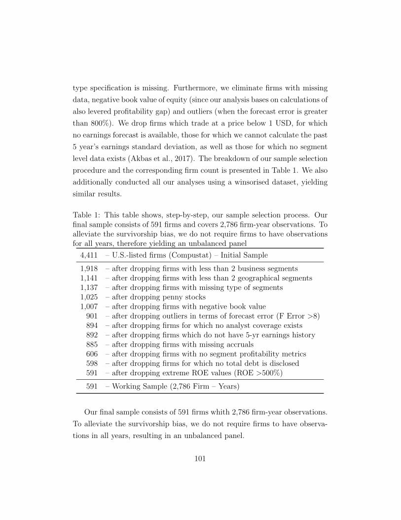
type specification is missing. Furthermore, we eliminate firms with missing
data, negative book value of equity (since our analysis bases on calculations of
also levered profitability gap) and outliers (when the forecast error is greater
than 800%). We drop firms which trade at a price below 1 USD, for which
no earnings forecast is available, those for which we cannot calculate the past
5 year’s earnings standard deviation, as well as those for which no segment
level data exists (Akbas et al., 2017). The breakdown of our sample selection
procedure and the corresponding firm count is presented in Table 1. We also
additionally conducted all our analyses using a winsorised dataset, yielding
similar results.
Table 1: This table shows, step-by-step, our sample selection process. Ourfinal sample consists of 591 firms and covers 2,786 firm-year observations. Toalleviate the survivorship bias, we do not require firms to have observationsfor all years, therefore yielding an unbalanced panel
4,411 – U.S.-listed firms (Compustat) – Initial Sample
1,918 – after dropping firms with less than 2 business segments1,141 – after dropping firms with less than 2 geographical segments1,137 – after dropping firms with missing type of segments1,025 – after dropping penny stocks1,007 – after dropping firms with negative book value
901 – after dropping outliers in terms of forecast error (F Error >8)894 – after dropping firms for which no analyst coverage exists892 – after dropping firms which do not have 5-yr earnings history885 – after dropping firms with missing accruals606 – after dropping firms with no segment profitability metrics598 – after dropping firms for which no total debt is disclosed591 – after dropping extreme ROE values (ROE >500%)
591 – Working Sample (2,786 Firm – Years)
Our final sample consists of 591 firms whith 2,786 firm-year observations.
To alleviate the survivorship bias, we do not require firms to have observa-
tions in all years, resulting in an unbalanced panel.
101

Table 2: This table presents descriptive statistics referring to our final sampleof 591 firms. A breakdown showing descriptive statistics for each variable ona year by year basis is available in Table 8 in the Appendix.
n m sd p25 p50 p75
F ERROR 2,790 0.051 0.132 0.007 0.019 0.044F ERROR (Sign) 2,790 -0.033 0.138 -0.035 -0.009 0.003ROA Gap1 2,790 0.035 0.176 0.001 0.006 0.021ROA Gap2 2,790 0.049 0.086 0.009 0.027 0.058ROA Gap3 2,790 0.031 0.059 0.006 0.017 0.036ROA Gap1 (Sign) 2,790 0.019 0.178 -0.004 0.000 0.009ROA Gap2 (Sign) 2,790 0.037 0.092 0.000 0.022 0.053ROA Gap3 (Sign) 2,790 0.020 0.063 0.000 0.013 0.031ROE Gap1 2,541 0.046 0.102 0.017 0.029 0.047ROE Gap2 2,541 0.035 0.047 0.012 0.024 0.043ROE Gap3 2,541 0.037 0.066 0.011 0.023 0.044ROE Gap1 (Sign) 2,541 -0.058 0.391 -0.109 -0.057 -0.023ROE Gap2 (Sign) 2,541 -0.059 0.233 -0.091 -0.039 0.003ROE Gap3 (Sign) 2,541 -0.030 0.236 -0.075 -0.023 0.027SplitBS 2,790 0.519 0.195 0.421 0.532 0.666SplitGS 2,790 0.467 0.227 0.300 0.491 0.657GranBS M 2,790 0.725 0.152 0.571 0.857 0.857GranBS D 2,790 0.427 0.119 0.368 0.421 0.474GranGS M 2,790 0.364 0.183 0.167 0.417 0.500GranGS D 2,790 0.331 0.075 0.276 0.345 0.345ACCRUALS 2,790 0.040 0.026 0.026 0.035 0.047NESTIMATES 2,790 0.215 0.154 0.098 0.176 0.314EPS STDEV 2,790 -0.080 1.174 -0.841 -0.170 0.519MARKET CAP 2,790 8,315 23,338 757 2,082 5,676ASSETS 2,790 9,491 39,627 764 2,255 5,957REVENUE 2,790 7,263 18,161 744 1,960 5,012DEBT TO EQUITY 2,790 0.835 1.587 0.180 0.481 0.880NSEGBUS 2,790 4.318 1.669 3 4 5NSEGGEO 2,790 4.767 3.496 3 4 6NNAICSBUS 2,790 4.007 2.029 3 4 5NNAICSGEO 2,790 1.853 0.399 2 2 2
102

5. Empirical Results
In this section we empirically investigate the relationship between seg-
ment reporting and analyst’s earnings forecast error. It is important to note,
that by construction, the forecast error throughout our analysis is depicted
as a delta Earnings-to-Price ratio. To get a benchmark for the magnitude
of the reported forecast errors, as well as to help in interpreting our results,
one might consider a normal Price-to-Earnings Ratio of 10, which translates
to Earnings-to-Price ratio of 0.1. While looking at Table 2, we report the
interquartile range for the forecast error at 0.044-0.007 or 0.037, which in
turn translates to 37% of a normal Earnings-to-Price ratio. Given this ob-
served magnitude, a better understanding of the drivers of earnings forecast
errors is of importance for all market participants, in particular to those who
heavily rely on earnings multiples for valuation or investment purposes.
5.1. Descriptive Statistics and Univariate Analysis
Table 2 reports the descriptive statistics for our working sample. We
report the correlation matrix in Tables 3 a and 3 b. For a complete description
of our variables and data sources please refer to Table 9 in the Appendix.
Forecast Error (denoted as delta earnings-to-price ratio): The
mean (median) absolute forecast error F ERROR scaled by price at time t
is 0.051 (0.019). If the sign of the forecast error is considered, the mean (me-
dian) value of the forecast error of the F ERROR(Sign) is -0.033 (-0.009).
Table 4, Panel A splits and ranks the different profitability gap variables ac-
cording to the forecast error quintiles. We observe that the higher quintiles
of F ERROR correspond to higher mean (median) profitability gaps, sug-
gesting that EPS forecasts might indeed be influenced by segment reporting.
However, the standard deviation of the profitability gaps is relatively high
when the profitability gaps are split and ranked according the F ERROR
and F ERROR (Sign). We analyze this relationship further in a multivari-
103

Tab
le3
a:T
his
table
cove
rsth
eco
rrel
atio
ns
bet
wee
nou
rse
lect
edva
riab
les.
Sp
earm
an(P
ears
on)
corr
elat
ions
are
rep
orte
db
elow
(ab
ove)
the
dia
gonal
,w
hile
bol
den
trie
sden
ote
sign
ifica
nce
atp<.0
5F
ER
RO
RF
ER
RO
R(S
ign)
RO
AG
ap1
RO
AG
ap2
RO
AG
ap3
RO
AG
ap1
(Sig
n)
RO
AG
ap2
(Sig
n)
RO
AG
ap3
(Sig
n)
RO
EG
ap1
RO
EG
ap2
RO
EG
ap3
RO
EG
ap1
(Sig
n)
RO
EG
ap2
(Sig
n)
RO
EG
ap3
(Sig
n)
Spli
tBS
Sp
litG
S
FE
RR
OR
1-0
.336
0.02
80.0
74
0.1
15
-0.0
69
-0.1
38
-0.1
17
0.1
17
0.3
02
0.2
50
-0.0
060.
035
0.01
00.
016
0.00
5F
ER
RO
R(S
ign
)-0
.573
1-0
.026
-0.0
68
-0.1
11
0.0
68
0.1
45
0.1
23
-0.1
04
-0.2
69
-0.2
21
0.00
9-0
.018
0.00
9-0
.025
-0.0
21R
OA
Gap
10.1
88
-0.1
65
10.3
98
0.4
86
0.9
30
0.1
10
0.2
04
0.7
09
0.2
27
0.1
83
0.7
38
0.0
49
0.03
30.0
48
0.00
8R
OA
Gap
20.
031
0.03
20.3
14
10.7
81
0.2
16
0.5
21
0.4
80
0.2
16
0.3
42
0.5
99
0.1
60
0.1
76
0.3
01
0.02
70.
012
RO
AG
ap3
0.0
88
-0.0
570.4
73
0.8
85
10.3
54
0.4
62
0.6
21
0.3
05
0.4
47
0.4
33
0.2
85
0.2
67
0.2
91
0.0
55
0.02
5R
OA
Gap
1(S
ign
)-0
.033
0.05
00.1
18
0.2
17
0.2
01
10.4
67
0.5
35
0.6
12
0.0
51
0.0
21
0.7
73
0.0
97
0.0
96
0.0
44
0.01
8R
OA
Gap
2(S
ign
)-0
.097
0.1
53
0.1
17
0.77
80.6
25
0.2
34
10.8
04
-0.0
71
-0.1
30
-0.1
41
0.1
63
0.3
01
0.5
29
0.02
10.0
39
RO
AG
ap3
(Sig
n)
-0.0
690.0
88
0.1
22
0.6
71
0.6
94
0.3
36
0.8
93
1-0
.035
-0.0
92
-0.0
53
0.2
77
0.4
35
0.4
97
0.03
70.0
48
RO
EG
ap1
0.1
33
0.01
80.2
10
0.05
90.
036
-0.2
04
-0.1
23
-0.1
99
10.6
90
0.5
48
0.4
38
-0.0
45
-0.0
67
0.03
7-0
.023
RO
EG
ap2
0.1
29
-0.0
300.1
66
0.04
90.
042
-0.1
44
-0.1
52
-0.2
12
0.5
13
10.7
90
0.00
8-0
.093
-0.1
22
0.03
5-0
.031
RO
EG
ap3
0.1
71
-0.0
92
0.1
91
0.1
81
0.2
09
-0.0
527
-0.0
25-0
.035
0.3
91
0.7
73
10.
013
-0.0
30-0
.050
0.01
3-0
.043
RO
EG
ap1
(Sig
n)
0.2
40
-0.2
40
0.2
12
0.06
60.1
82
0.4
50
0.1
85
0.3
34
-0.4
64
-0.2
91
-0.1
56
10.8
33
0.6
82
0.01
70.
014
RO
EG
ap2
(Sig
n)
0.2
36
-0.2
43
0.1
68
0.3
37
0.4
57
0.3
17
0.4
74
0.6
31
-0.4
45
-0.3
35
-0.0
97
0.4
95
10.9
03
-0.0
120.
018
RO
EG
ap3
(Sig
n)
0.2
04
-0.1
62
0.1
53
0.5
37
0.5
12
0.3
34
0.6
76
0.6
93
-0.3
85
-0.3
37
-0.1
00
0.4
30
0.9
28
1-0
.005
0.02
1S
pli
tBS
-0.0
390.
033
0.06
90.
011
0.03
110.
081
0.05
10.
074
0.02
2-0
.053
-0.0
460.
014
-0.0
01-0
.001
10.1
40
Sp
litG
S0.
001
-0.0
140.0
84
-0.0
27-0
.038
0.0
99
0.01
00.
023
-0.0
54-0
.059
-0.0
83
0.00
5-0
.039
-0.0
430.1
65
1G
ran
BS
M-0
.030
0.04
70.
018
0.1
39
0.1
32
-0.0
94
0.1
24
0.1
06
-0.0
71-0
.088
-0.0
85
-0.0
183
0.1
03
0.1
09
-0.1
50
-0.2
24
Gra
nB
SD
-0.0
230.
009
-0.1
09
0.04
80.
054
0.06
40.1
09
0.1
38
-0.0
21-0
.058
-0.0
39-0
.020
30.
045
0.06
-0.1
29
-0.1
39
Gra
nG
SM
0.03
9-0
.004
-0.0
51-0
.023
-0.0
23-0
.081
0.02
20.
020
-0.0
46-0
.130
-0.1
38
0.06
40.1
19
0.0
98
-0.0
70-0
.201
Gra
nG
SD
-0.0
690.
063
-0.1
47
-0.0
60-0
.082
-0.0
770.
006
-0.0
210.0
91
-0.0
11-0
.040
-0.1
52
-0.0
97
-0.0
57-0
.031
0.0
86
AC
CR
UA
LS
0.1
46
-0.2
06
0.05
80.
0558
0.05
3-0
.011
0.01
9-0
.008
-0.0
34-0
.014
0.00
80.1
04
0.1
56
0.1
59
-0.1
18
-0.1
02
NE
ST
IMA
TE
S-0
.186
0.06
030.
044
-0.0
03-0
.057
0.1
15
0.00
4-0
.012
0.04
30.
059
0.06
8-0
.180
-0.2
08
-0.1
56
0.2
12
0.2
86
EP
SS
TD
EV
0.2
12
-0.0
780.1
10
0.0
97
0.0
96
0.1
40
0.1
02
0.0
97
0.04
80.1
04
0.1
30
0.1
11
0.1
07
0.1
21
0.0
92
0.07
4M
AR
KE
TC
AP
-0.3
49
0.2
03
0.06
90.
014
-0.0
470.1
40
0.05
10.
011
0.04
00.
027
-0.0
25-0
.257
-0.2
93
-0.2
36
0.1
66
0.3
84
AS
SE
TS
-0.1
51
0.0
84
0.08
0-0
.067
-0.1
08
0.1
30
-0.0
42-0
.064
0.1
94
0.1
46
0.1
02
-0.2
41
-0.2
94
-0.2
61
0.1
76
0.3
60
RE
VE
NU
E-0
.197
0.1
40
0.08
00.
008
-0.0
540.1
25
0.02
4-0
.024
0.2
71
0.1
58
0.0
95
-0.3
23
-0.3
56
-0.2
85
0.1
60
0.2
82
DE
BT
TO
EQ
UIT
Y0.
040
-0.0
91
0.00
7-0
.054
-0.0
650.
008
-0.0
15-0
.046
0.2
06
0.1
58
0.1
67
-0.3
24
-0.2
13
-0.1
63
0.02
30.
025
NS
EG
BU
S-0
.015
0.1
20
0.14
30.1
63
0.1
62
0.1
12
0.1
98
0.1
83
0.03
5-0
.032
-0.0
24-0
.001
0.01
90.
057
0.6
53
0.1
44
NS
EG
GE
O0.
057
-0.0
89
0.1
04
0.01
2-0
.041
0.1
15
0.04
80.
013
-0.0
89
-0.0
36-0
.056
0.1
06
0.03
50.
051
0.1
94
0.7
27
NN
AIC
SB
US
0.04
9-0
.060
0.04
4-0
.085
-0.1
22
0.1
07
-0.0
15-0
.049
-0.0
60-0
.123
-0.0
99
0.04
70.
008
0.03
00.1
07
0.06
8N
NA
ICS
GE
O-0
.035
-0.0
24-0
.010
-0.0
18-0
.073
0.08
00.
029
-0.0
23-0
.079
-0.0
84
-0.0
540.
060
0.00
30.
040
-0.0
100.
077
104
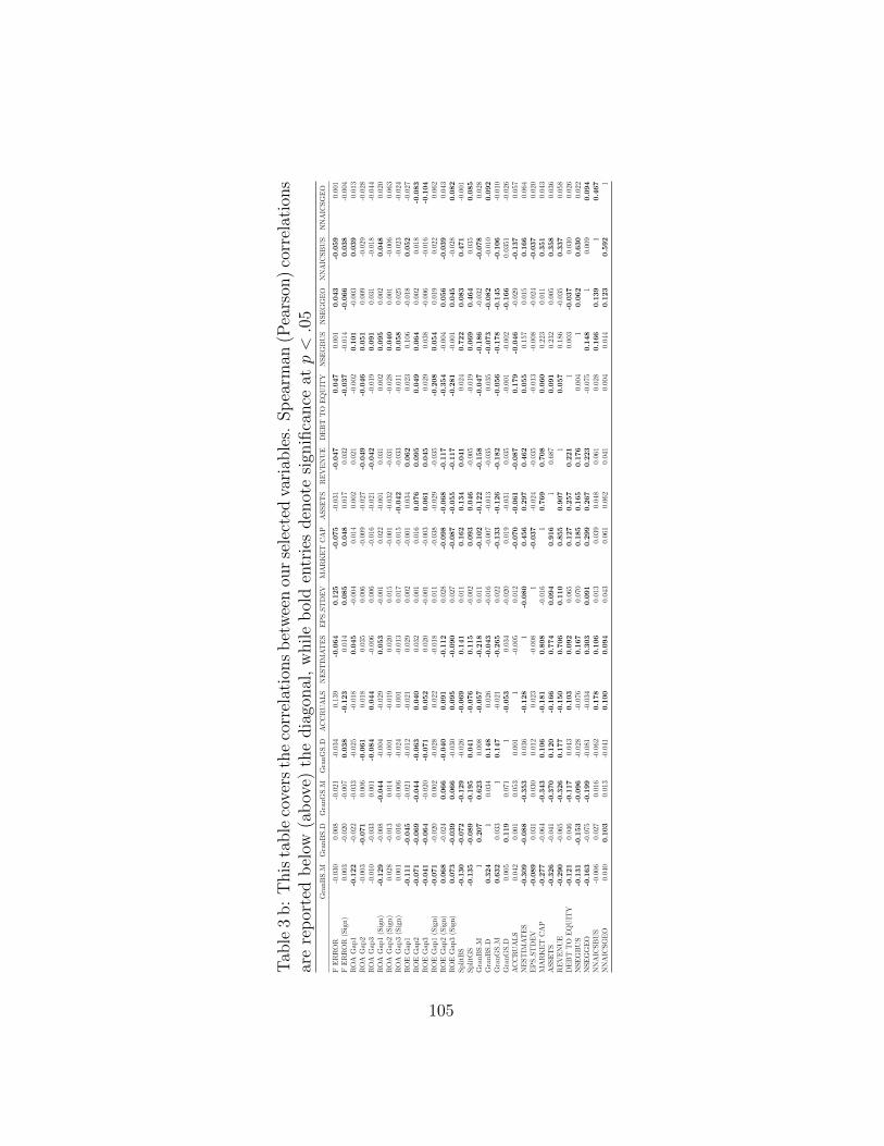
Tab
le3
b:
This
table
cove
rsth
eco
rrel
atio
ns
bet
wee
nou
rse
lect
edva
riab
les.
Sp
earm
an(P
ears
on)
corr
elat
ions
are
rep
orte
db
elow
(ab
ove)
the
dia
gonal
,w
hile
bol
den
trie
sden
ote
sign
ifica
nce
atp<.0
5G
ran
BS
MG
ran
BS
DG
ran
GS
MG
ran
GS
DA
CC
RU
AL
SN
ES
TIM
AT
ES
EP
SS
TD
EV
MA
RK
ET
CA
PA
SS
ET
SR
EV
EN
UE
DE
BT
TO
EQ
UIT
YN
SE
GB
US
NS
EG
GE
ON
NA
ICS
BU
SN
NA
ICS
GE
O
FE
RR
OR
-0.0
300.
008
-0.0
21-0
.034
0.13
9-0
.064
0.1
25
-0.0
75
-0.0
31-0
.047
0.0
47
0.00
10.0
43
-0.0
59
0.00
1F
ER
RO
R(S
ign
)0.
003
-0.0
20-0
.007
0.0
38
-0.1
23
0.01
40.0
85
0.0
48
0.01
70.
032
-0.0
37
-0.0
14-0
.066
0.0
38
-0.0
04R
OA
Gap
1-0
.122
-0.0
22-0
.033
-0.0
25-0
.018
0.0
45
-0.0
040.
014
0.00
20.
021
-0.0
020.1
01
-0.0
030.0
39
0.01
3R
OA
Gap
2-0
.003
-0.0
71
0.00
6-0
.061
0.01
80.
035
0.00
6-0
.009
-0.0
27-0
.049
-0.0
46
0.0
51
0.00
9-0
.029
-0.0
28R
OA
Gap
3-0
.010
-0.0
330.
001
-0.0
84
0.0
44
-0.0
060.
006
-0.0
16-0
.021
-0.0
42
-0.0
190.0
91
0.03
1-0
.018
-0.0
44R
OA
Gap
1(S
ign
)-0
.129
-0.0
08-0
.044
-0.0
04-0
.029
0.0
53
-0.0
010.
022
-0.0
010.
031
0.00
20.0
95
0.00
20.0
48
0.02
0R
OA
Gap
2(S
ign
)0.
028
-0.0
130.
014
-0.0
01-0
.019
0.02
00.
015
-0.0
01-0
.032
-0.0
31-0
.028
0.0
40
0.00
1-0
.006
0.06
3R
OA
Gap
3(S
ign
)0.
001
0.01
6-0
.006
-0.0
240.
001
-0.0
130.
017
-0.0
15-0
.042
-0.0
33-0
.011
0.0
58
0.02
5-0
.023
-0.0
24R
OE
Gap
1-0
.111
-0.0
45
-0.0
21-0
.012
-0.0
210.
029
0.00
2-0
.001
0.03
40.0
62
0.02
30.
106
-0.0
180.0
52
-0.0
27R
OE
Gap
2-0
.071
-0.0
69
-0.0
44
-0.0
63
0.0
40
0.03
20.
001
0.01
60.0
76
0.0
95
0.0
49
0.0
64
0.00
20.
018
-0.0
83
RO
EG
ap3
-0.0
41
-0.0
64
-0.0
20-0
.071
0.0
52
0.02
0-0
.001
-0.0
030.0
61
0.0
45
0.02
90.
038
-0.0
06-0
.016
-0.1
04
RO
EG
ap1
(Sig
n)
-0.0
71
-0.0
200.
002
-0.0
280.
022
-0.0
180.
011
-0.0
38-0
.029
-0.0
35-0
.208
0.0
54
0.01
90.
022
0.06
2R
OE
Gap
2(S
ign
)0.0
68
-0.0
240.0
66
-0.0
40
0.0
91
-0.1
12
0.02
8-0
.098
-0.0
68
-0.1
17
-0.3
54
-0.0
040.0
56
-0.0
39
0.04
3R
OE
Gap
3(S
ign
)0.0
73
-0.0
39
0.0
66
-0.0
300.0
95
-0.0
90
0.02
7-0
.087
-0.0
55
-0.1
17
-0.2
81
-0.0
010.0
45
-0.0
280.0
82
Sp
litB
S-0
.130
-0.0
72
-0.1
29
-0.0
26-0
.069
0.1
41
0.01
10.1
62
0.1
34
0.0
41
0.02
40.7
22
0.0
83
0.4
71
-0.0
01S
pli
tGS
-0.1
35
-0.0
89
-0.1
95
0.0
41
-0.0
76
0.1
15
-0.0
020.0
93
0.0
46
-0.0
05-0
.019
0.0
69
0.4
64
0.03
50.0
85
Gra
nB
SM
10.2
07
0.6
23
0.00
8-0
.057
-0.2
18
0.01
1-0
.102
-0.1
22
-0.1
58
-0.0
47
-0.1
86
-0.0
32-0
.078
0.02
8G
ran
BS
D0.3
24
10.
034
0.1
48
0.02
6-0
.043
-0.0
16-0
.007
-0.0
13-0
.035
0.03
5-0
.073
-0.0
82
-0.0
100.0
92
Gra
nG
SM
0.6
32
0.03
31
0.1
47
-0.0
21-0
.265
0.02
2-0
.133
-0.1
26
-0.1
82
-0.0
56
-0.1
78
-0.1
45
-0.1
06
-0.0
10G
ran
GS
D0.
005
0.1
19
0.07
11
-0.0
53
0.03
4-0
.020
0.01
9-0
.031
0.03
5-0
.001
-0.0
02-0
.166
0.03
51-0
.026
AC
CR
UA
LS
0.04
20.
001
0.05
30.
001
1-0
.005
0.01
2-0
.070
-0.0
61
-0.0
87
0.1
79
-0.0
46
-0.0
29-0
.137
0.05
7N
ES
TIM
AT
ES
-0.3
09
-0.0
88
-0.3
53
0.03
6-0
.128
1-0
.080
0.4
56
0.2
97
0.4
62
0.0
55
0.15
70.
015
0.1
66
0.06
4E
PS
ST
DE
V-0
.089
0.03
10.
030
0.01
20.
023
-0.0
081
-0.0
37
-0.0
24-0
.035
-0.0
13-0
.008
-0.0
24-0
.037
0.02
0M
AR
KE
TC
AP
-0.2
77
-0.0
64-0
.343
0.1
06
-0.1
81
0.8
08
-0.0
161
0.7
69
0.7
08
0.0
60
0.22
30.
011
0.3
51
0.04
3A
SS
ET
S-0
.326
-0.0
41-0
.370
0.1
20
-0.1
66
0.7
74
0.0
94
0.9
16
10.
687
0.0
91
0.23
20.
005
0.3
58
0.03
6R
EV
EN
UE
-0.2
90
-0.0
65-0
.326
0.1
77
-0.1
50
0.7
06
0.1
10
0.8
55
0.9
07
10.0
57
0.18
6-0
.035
0.3
37
0.05
8D
EB
TT
OE
QU
ITY
-0.1
21
0.04
6-0
.117
0.04
30.1
03
0.0
92
0.06
50.1
27
0.2
57
0.2
21
10.
003
-0.0
37
0.03
00.
026
NS
EG
BU
S-0
.131
-0.1
53
-0.0
96
-0.0
28-0
.076
0.1
67
0.07
00.1
85
0.1
65
0.1
76
0.00
41
0.0
62
0.6
30
0.02
2N
SE
GG
EO
-0.1
63
-0.0
75-0
.199
-0.0
81-0
.034
0.3
03
0.0
91
0.2
99
0.2
67
0.2
23
-0.0
750.1
48
10.
009
0.0
94
NN
AIC
SB
US
-0.0
060.
027
0.01
6-0
.062
0.1
78
0.1
06
0.01
30.
039
0.04
80.
061
0.02
80.1
66
0.1
39
10.4
67
NN
AIC
SG
EO
0.04
00.1
03
0.01
3-0
.041
0.1
00
0.0
94
0.04
30.
061
0.06
20.
041
0.00
40.
044
0.1
23
0.5
92
1
105

ate setting in Section 5.2.
Moreover, Table 4 Panel A reveals that the standard deviation of 0.132
(and similar 0.138 for F ERROR(Sign)) is primarily driven by the fifth
quintile, which is the one with the largest forecast error. The negative values
reported for the mean of F ERROR(Sign) across quintiles one two and three
indicate that a substantial proportion of the firms included in our sample
exhibit overly optimistic (pessimistic) earnings forecasts corresponding to
the profitability gaps, whereby actual EPS figures undershoot (overshoot)
analysts’ expectations.
Profitability Gap (between aggregated profitability from seg-
ments and firm profitability): The mean (median) absolute unlevered
profitability gaps ROAGap1, ROAGap2, ROAGap3 are reported at 0.035
(0.006), 0.049 (0.027), 0.031 (0.017). The mean (median) levered profitabil-
ity gaps denoted by ROEGap1, ROEGap2, ROEGap3 are 0.046 (0.029),
0.035 (0.024), 0.037 (0.023). Considering also the direction (sign) of the gap,
the mean (median) reported unlevered profitability gaps ROAGap1(Sign),
ROAGap2(Sign), ROAGap3(Sign) and the mean (median) levered prof-
itability gapsROEGap1(Sign), ROEGap2(Sign), ROEGap3(Sign) are 0.019
(0.000), 0.037 (-0.022), 0.020 (-0.013) and -0.058 (-0.057), -0.059 (-0.039), -
0.030 (-0.023), respectively. These results provide initial evidence that the
aggregated profitability from segments is higher than the profitability from
the consolidated financial statements, which suggests that if analysts rely
too much on segments reporting their EPS estimates might overestimate the
profitability of assets, equity, as well as the firm’s earnings. Again the stan-
dard deviation is high, further analysis is carried out in a multivariate setting
(see section regression analysis).
Table 4, Panel B splits and ranks the unlevered profitability gap according
to the forecast error when the sign of the forecast error F ERROR(Sign)
is also taken into account. The figures in the reported quintiles suggest
that overly optimistic (pessimistic) EPS estimates correspond to observa-
106

tions where segment aggregated profitability is indeed higher (lower) than
consolidated profitability. Further evidence is also provided when considering
the Spearman (Pearson) correlations reported in Table 3 a. Specifically, the
Spearman (Pearson) between the absolute forecast error F ERROR and the
levered (ROE) profitability gap metrics ROEGap1, ROEGap2, ROEGap3
is 0.133 (0.117), 0.129 (0.302) and 0.171 (0.250), while if the sign is also tak-
ing into account, then the correlations are: 0.240 (-0.006), 0.236 (0.035) and
0.204 (0.010), respectively.
Segment Split: The mean (median) business segment split variable
SplitBS is 0.519 (0.532), while geographical segment split variable SplitGS
is 0.467 (0.491).
Line Item Granularity: The mean (median) business segment granu-
larity of mandatory GranBS M and discretionary line items GranBS D are
0.725 (0.857) and 0.427 (0.421), respectively. The mean (median) geograph-
ical segment granularity covering mandatory GranGS M and discretionary
line items GranGS D are 0.364 (0.417) and 0.331 (0.345), respectively.
Number of segments and industries: The mean (median) number of
business segments, denoted as NSEGBUS, is 4.318 (4.0) with a standard
deviation of 1.669, while the mean (median) number of geographical seg-
ments, NSEGGEO, is 4.767 (4.0) with a standard deviation of 3.496. The
mean (median) reported number of NAICS per company across business seg-
ments, denoted as NNAICSBUS, is 4.007 (4.0) with a standard deviation
of 2.029, while in the case of geographical segments, NNAICSGEO, the
mean (median) is 1.853 (2.0) with a standard deviation of 0.399.
Table 5 Panel A splits and ranks the segment split variables: SplitBS,
SplitGS and the line item granularity variables: GranBS M , GranBS D,
GranGS M , and GranGS D according to the calculated forecast error quin-
tiles of F ERROR. Based on the correlation tables and contrary to the
common expectation that an increased split would increase valuable infor-
mation on business activities and facilitate the forecast of earnings, we find
107

Tab
le4:
This
table
splits
and
ranks
the
six
pro
fita
bilit
yga
pva
riab
les
acco
rdin
gto
the
ranke
dquin
tile
sof
the
abso
lute
fore
cast
erro
r(P
anel
A),
asw
ell
asth
era
wfo
reca
ster
ror
(Pan
elB
).T
he
figu
res
inth
ere
por
ted
quin
tile
ssu
gges
tth
atov
erly
opti
mis
tic
(pes
sim
isti
c)E
PS
fore
cast
sco
rres
pon
dto
obse
rvat
ions
wher
ese
gmen
tag
greg
ated
pro
fita
bilit
yis
indee
dhig
her
(low
er)
than
conso
lidat
edpro
fita
bilit
y.P
anel
A:
Abso
lute
fore
cast
erro
r
FE
RR
OR
RO
AG
ap1
RO
AG
ap2
RO
AG
ap3
RO
EG
ap1
RO
EG
ap2
RO
EG
ap3
Quin
tile
nm
sdm
sdm
sdm
sdm
sdm
sdm
sd1
558
0.00
20.
001
0.02
80.
222
0.05
00.
084
0.02
70.
046
0.03
60.
076
0.02
70.
032
0.02
80.
041
255
80.
009
0.00
20.
036
0.21
80.
048
0.06
40.
027
0.03
70.
041
0.09
50.
028
0.02
70.
029
0.03
53
558
0.01
90.
004
0.03
80.
181
0.05
10.
105
0.03
30.
093
0.04
30.
078
0.03
10.
030
0.03
20.
033
455
80.
038
0.00
80.
028
0.09
30.
045
0.06
40.
029
0.04
20.
046
0.12
90.
032
0.02
90.
035
0.03
85
558
0.18
90.
251
0.04
30.
127
0.05
30.
105
0.03
90.
056
0.06
50.
120
0.05
60.
084
0.06
30.
127
Tot
al27
900.
051
0.13
20.
035
0.17
60.
049
0.08
60.
031
0.05
90.
046
0.10
20.
035
0.04
70.
037
0.06
6
Pan
elB
:F
orec
ast
erro
rco
nsi
der
ing
the
sign
FE
RR
OR
(Sig
n)
RO
AG
ap1
(Sig
n)
RO
AG
ap2
(Sig
n)
RO
AG
ap3(
Sig
n)
RO
EG
ap1
(Sig
n)
RO
EG
ap2
(Sig
n)
RO
EG
ap3
(Sig
n)
Quin
tile
nm
sdm
sdm
sdm
sdm
sdm
sdm
sd1
558
-0.1
720.
199
-0.0
110.
080
0.01
20.
115
0.00
80.
068
-0.0
600.
225
-0.0
260.
217
-0.0
140.
243
255
8-0
.028
0.00
80.
019
0.09
40.
037
0.06
20.
022
0.04
3-0
.047
0.24
2-0
.039
0.17
9-0
.011
0.19
53
558
-0.0
090.
004
0.03
20.
201
0.05
00.
114
0.02
70.
095
-0.0
410.
410
-0.0
550.
210
-0.0
220.
221
455
80.
002
0.00
30.
023
0.22
10.
043
0.07
80.
022
0.04
5-0
.087
0.45
7-0
.089
0.25
7-0
.056
0.25
15
558
0.04
50.
170
0.03
40.
230
0.04
40.
074
0.02
20.
046
-0.0
520.
529
-0.0
830.
284
-0.0
480.
260
Tot
al27
90-0
.033
0.13
80.
019
0.17
80.
037
0.09
20.
020
0.06
3-0
.058
0.39
1-0
.059
0.23
3-0
.030
0.23
6
108

Tab
le5:
Pan
elA
ofth
ista
ble
splits
and
ranks
the
segm
ent
split
vari
able
san
dth
eline
item
gran
ula
rity
vari
able
sac
cord
ing
toth
eab
solu
tefo
reca
ster
ror
quin
tile
s.P
anel
Bsp
lits
and
ranks
the
vari
able
sre
ferr
ing
toth
enum
ber
ofbusi
nes
sse
gmen
ts,
busi
nes
sN
AIC
S,
man
dat
ory
and
dis
cret
ionar
yline
item
gran
ula
rity
acco
rdin
gto
segm
ent
split
quin
tile
s.P
anel
A
FE
RR
OR
Sp
litB
SS
pli
tGS
Gra
nB
SM
Gra
nB
SD
Gra
nG
SM
Gra
nG
SD
Sp
litB
SN
NA
ICS
BU
S
Qu
inti
len
msd
msd
msd
msd
msd
msd
msd
msd
msd
155
80.
002
0.00
10.
530
0.19
50.
467
0.22
30.
733
0.15
00.
439
0.11
80.
317
0.15
70.
207
0.05
20.
530
0.19
54.
172
2.17
92
558
0.00
90.
002
0.51
80.
196
0.45
70.
221
0.72
50.
151
0.42
40.
110
0.31
20.
155
0.20
10.
041
0.51
80.
196
4.19
92.
302
355
80.
019
0.00
40.
518
0.19
70.
483
0.22
30.
728
0.15
60.
419
0.11
20.
314
0.15
50.
198
0.04
10.
518
0.19
73.
973
1.91
44
558
0.03
80.
008
0.51
50.
202
0.46
50.
235
0.71
80.
156
0.42
50.
121
0.31
70.
157
0.20
00.
045
0.51
50.
202
3.92
71.
973
555
80.
189
0.25
10.
514
0.18
50.
462
0.23
40.
720
0.14
90.
428
0.13
10.
302
0.15
90.
195
0.04
60.
514
0.18
53.
763
1.69
6T
otal
2790
0.05
10.
132
0.51
90.
195
0.46
70.
227
0.72
50.
152
0.42
70.
119
0.31
20.
157
0.20
00.
045
0.51
90.
195
4.00
72.
029
Pan
elB
Sp
litB
SN
SE
GB
US
NN
AIC
SB
US
Gra
nB
SM
Gra
nB
SD
Gra
nG
SM
Gra
nG
SD
Qu
inti
len
msd
msd
msd
msd
msd
msd
msd
155
80.
209
0.11
02.
944
0.82
53.
043
1.07
60.
751
0.14
10.
439
0.15
20.
337
0.15
70.
205
0.04
82
558
0.44
80.
033
3.31
20.
788
3.15
21.
089
0.75
10.
140
0.43
50.
104
0.32
90.
151
0.19
50.
055
355
80.
538
0.03
53.
975
0.93
03.
525
1.50
90.
712
0.16
60.
423
0.12
20.
313
0.15
50.
200
0.03
64
558
0.64
70.
024
4.80
50.
891
4.48
61.
844
0.71
10.
153
0.42
00.
103
0.31
00.
166
0.20
40.
042
555
80.
754
0.04
56.
552
1.65
05.
828
2.67
20.
699
0.15
30.
418
0.10
50.
273
0.14
70.
197
0.04
3T
otal
2790
0.51
90.
195
4.31
81.
669
4.00
72.
029
0.72
50.
152
0.42
70.
119
0.31
20.
157
0.20
00.
045
109

no apparent relationship between these metrics, at least based on this anal-
ysis. A possible explanation might be that the increased segment split is
actually reflecting more diversified firms and offsets the information value of
a greater segment split. However, the number of NAICS, NNAICSBUS,
is quasi-constant throughout all quintiles, close to 4, with only a slight de-
crease in the mean and standard deviation when considering the 5 quintiles of
F ERROR. Moreover, the correlation matrix does not suggest a strong as-
sociation between diversification and the forecast error,while the correlation
between the forecast error and the number of reported NAICS is negligibly
low, as well as showing an inconclusive sign 0.049 (-0.059).
Segment split is often used as a proxy for (or confused with) diversification
(e.g., Kang et al., 2017), despite the discretionary character of the actual
segment split. To display the relationship between segment split, number of
business segments and number of industries reported for business segments,
Table 5, Panel B splits and ranks number of segments and the number of
line items and NAICS against our segment split variable. Table 6 shows
the number of NAICS for business segments and the number of segments
and segment split for the corresponding firms. It reveals that a striking 71.4
percent of the firms operate in one, two, three or four industries but report,
on average, in all cases only about the same number of segments and the same
segment split. Moreover, in line with this argumentation, the increase in the
average segment split from 0.209 to 0.538, as depicted in Table5 in Panel B,
referring to quintiles one to three (covering 60% of all firms) corresponds to
firms having three to four business segments and reporting approximately
three business NAICS.
Furthermore, when looking at the relation between the forecast error and
the number of business segments, we find similar results, namely a correlation
of -0.015 (0.001). Given a mean (median) of business segments and NAICS of
about 4, the correlation between the segment split variable and the number
of business segments is 0.653 (0.722); however, the correlation between the
110

Table 6: This table provides an overview of the number of business NAICSthat firms in our data-set report and relates this number to the number ofreported business segments and segment split.
NNAICS BUS NSEGBUS SplitBS
Nr. Firms Perc. Cum. m sd m sd1 95 3.4 3.4 3.621 0.121 0.455 0.0222 480 17.2 20.6 3.567 0.060 0.435 0.0083 765 27.4 48.0 3.566 0.042 0.448 0.0074 653 23.4 71.4 4.044 0.050 0.499 0.007
5 296 10.6 82.0 5.091 0.065 0.610 0.0086 185 6.6 88.7 5.627 0.105 0.659 0.0097 139 5.0 93.7 5.957 0.092 0.699 0.0088 78 2.8 96.5 5.705 0.141 0.681 0.0099 40 1.4 97.9 7.225 0.233 0.698 0.02310 27 1.0 98.9 7.481 0.386 0.767 0.01011 16 0.6 99.4 8.938 0.536 0.808 0.01912 5 0.2 99.6 8.800 0.200 0.833 0.02013 2 0.1 99.7 9.500 0.500 0.851 0.00514 2 0.1 99.8 10.500 0.500 0.854 0.01015 4 0.1 99.9 10.750 0.250 0.864 0.01016 1 0.0 99.9 9.000 . 0.819 .17 2 0.1 100.0 15.000 0.000 0.916 0.001
Total 2790 100 4.317 0.072 0.519 0.008
Sub Group of NNAICSBUS 1 to 4: 3.726 0.053 0.462 0.008Sub Group of NNAICSBUS 5 to 17: 5.794 0.119 0.662 0.010
111

segment split and the number of NAICS is 0.107 (0.471), a substantially lower
value by comparison, supporting our understanding that it is important to
distinguish between segment split and diversification.
The analysis in Table 5, Panel B also provides evidence that an increased
number of segments results in a decreased number of reported line items when
the segment split increases, particularly for the quintiles 4 and 5, which is in
line with the finding in prior studies ((Bugeja et al., 2015; Ettredge et al.,
2006; Gotti, 2016). Also, when looking at the correlation figures in Table 3
a, the segment split, mandatory and discretionary line items are not linked
to a reduction in the forecast error in this univariate setting -0.039, -0.030,
-0.023 (0.016, -0.030, 0.008).
Size: The mean (median) size as measured through market capitalization
MARKET CAP is 8,315 (2,082) million USD with a standard deviation of
23,338, asset size ASSETS is 9,491 (2,255) million USD with a standard
deviation of 39,627 and revenue REV ENUE is 7,263 (1,960) million USD
with a standard deviation of 18,161.
There is a slight negative correlation between the accounting quality vari-
able ACCRUALS and the business segment split SplitBS of -0.118 (-0.069),
whereby the higher the split, the lower the number of disclosed mandatory
line items -0.150 (-.130). A similar picture is documented when looking at the
negative correlation between the geographical segment split and mandatory
line items granularity -.224 (-0.195), implying that an increased segment
split is correlated with a reduction in line items (Bugeja et al., 2015; Et-
tredge et al., 2006; Gotti, 2016). Conversely, when looking at discretionary
line items, the opposite can be observed.
Larger companies, as measured by market cap, total assets or revenue
benefit from increased analyst coverage as evidenced by correlations between
0.706 and 0.808 (0.297 and 0.462).
The forecast error positively correlates with standard deviation of last
five years of EPS 0.212 (0.125). In contrast to existing findings referring to
112
the impact of leverage on information availability (Dhaliwal et al., 2011), the
debt-to-equity ratio does not correlate with the forecast error 0.040 (0.047),
nor with the segment split -0.039 (0.016) in this univariate setting.
5.2. Regression Analysis
Table 7 depicts the results of our regression analysis. Panel A and Panel
B of Table 7 document and quantify the effect of the profitability gaps on
the forecast error. All of the 4 regressions address the relationship between
the profitability gap from “no-full-story” segments, for which profitability
reporting is incomplete, i.e. segments that do not report revenue or assets:
ROA Gap2, ROE Gap2, or segments lacking revenue, assets or operating
income: ROA Gap3 and ROE Gap3 and its effect on the forecast error. We
find and document a statistically significant (coefficient for the levered met-
ric is 0.797 for ROE Gap2) positive association with the forecast error. This
comes to support our fourth hypothesis (H4). This finding suggests that ana-
lysts’ earnings forecasts are biased towards firm profitability as derived from
segments, for which a complete set of profitability-related data items (assets,
revenues or operating earnings) is disclosed, the ”full-story” segments. More-
over, this finding is significantly tied to the amount and even the sign of the
earnings forecast error–statistically and economically significant coefficients
of PrftGap(SegPrft > ConsPrft), R-squared of 0.46, reported in Panel B
of Table 7. PrftGap(SegPrft > ConsPrft) captures the case, where the
aggregated segment reporting profitability is more optimistic than the prof-
itability based on consolidated financial statements. However, in the opposite
case, this is not the case. This implies that if aggregated segment profitabil-
ity (from ”full-story” segments) is higher than the consolidated profitability,
then analysts are inclined to issue overly optimistic earnings forecasts.
This suggests that the attention of analysts might be directed to those
segments where performance metrics are readily available. Our findings com-
plement prior research which shows that the discretion of segment reports
113

and usefulness of actual segment data is exploited by management, suggest-
ing that companies manage segment profitability through the allocation of
business activities when aggregating them into reported segments (Berger
and Hann, 2007) and inter-segment income shifting (Lail et al., 2014; You,
2014).
Referring to the non-GAAP vs GAAP topic, given the lack of a complete
reconciliation requirement between aggregated segments and firm level re-
porting, as well as the leeway provided by the low reporting requirements,
coupled with the internal measurement principle, we tested if the existence of
a discrepancy between segment aggregated profitability and firm level prof-
itability explains the forecast error ROA Gap1, ROE Gap1. However, the
evidence for a profitability gap that results from non-GAAP accounting (in-
ternal recognition and measurement principles for reported segments in con-
trast to the U.S.-GAAP for consolidated financial statements) is weak and
only supports H3 in the case of the levered metric, ROE Gap1, contrasting
the findings in Wang and Ettredge (2015) who report a value relevant re-
lationship with this gap. This could result from the firms’ use of external
accounting principles for their internal and segment reporting, facilitating
the preparation of segment reporting and internal reports as it is readily
available (Crawford et al., 2012; Nichols et al., 2012).
Throughout all of our different model specifications we find statistically
significant evidence that the segment split is positively associated with the
forecast error. To make sure that the findings are not driven by the level of
firm diversification, we control for firm diversification by creating dummies
for the number of business NAICS of a firm. The finding directly supports
our first hypothesis (H1) and strengthens the idea that an increased segment
split under the loose and permissive regulatory framework in defining and ag-
gregating business activities into reporting business segments does not serve
as a catalyst for forecasting purposes.
Referring to the coefficients of GranBS M and GranBS D, we find that
114
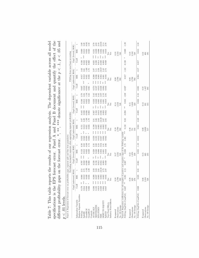
Tab
le7:
This
table
rep
orts
the
resu
lts
ofou
rre
gres
sion
anal
ysi
s.T
he
dep
enden
tva
riab
leac
ross
all
model
spec
ifica
tion
sis
the
EP
Sfo
reca
ster
ror.
Pan
elA
and
Pan
elB
docu
men
tan
dquan
tify
the
effec
tof
the
diff
eren
tpro
fita
bilit
yga
ps
onth
efo
reca
ster
ror.
*,**
,**
*den
ote
sign
ifica
nce
atth
ep<.1
,p<.0
5an
dp<.0
1le
vels
.P
anel
A:
Reg
ress
ion
offo
reca
ster
ror
onp
rofi
tab
ilit
yga
ps,
segm
ent
spli
tan
dli
ne
item
gran
ula
rity
Excl
ud
ing
inco
mp
lete
segm
ents
wh
enag
greg
atin
gse
gmen
tp
rofi
tab
ilit
yP
rftG
apfr
omn
on-G
aap
acco
unti
ng
Gap
2(u
nle
vere
d,
RO
A)
Gap
2(l
ever
ed,
RO
E)
Gap
3(u
nle
vere
d,
RO
A)
Gap
3(l
ever
ed,
RO
E)
Gap
1(u
nle
vere
d,
RO
A)
Gap
1(l
ever
ed,
RO
E)
Ind
epen
den
tV
aria
ble
Coeff
RS
Et
Coeff
RS
Et
Coeff
RS
Et
Coeff
RS
Et
Coeff
RS
Et
Coeff
RS
Et
Bu
sin
ess
Seg
men
tV
aria
ble
sP
rftG
ap0.
170
**0.
068
2.51
0.79
7**
*0.
123
6.50
0.25
2*
0.15
11.
670.
445
***
0.16
02.
790.
027
0.01
71.
630.
130
*0.
069
1.89
Sp
litB
S0.
044
***
0.01
23.
710.
032
***
0.01
22.
630.
040
***
0.01
23.
390.
038
***
0.01
23.
040.
042
***
0.01
23.
610.
043
***
0.01
33.
20G
ran
BS
M-0
.040
*0.
020
-1.9
3-0
.020
0.02
2-0
.89
-0.0
38*
0.02
1-1
.86
-0.0
260.
022
-1.1
6-0
.034
0.02
1-1
.60
-0.0
220.
024
-0.9
2G
ran
BS
D0.
066
*0.
035
1.89
0.06
8*
0.03
91.
740.
063
*0.
035
1.79
0.06
50.
040
1.63
0.06
1*
0.03
51.
750.
060
0.04
01.
50C
ontr
ols
AC
CR
UA
LS
0.58
6**
*0.
200
2.93
0.53
8**
0.22
82.
350.
559
***
0.19
92.
810.
567
**0.
233
2.43
0.57
4**
*0.
200
2.87
0.62
5**
*0.
231
2.70
NE
ST
IMA
TE
S0.
185
***
0.03
75.
030.
156
***
0.04
03.
920.
185
***
0.03
75.
060.
164
***
0.04
04.
060.
187
***
0.03
65.
110.
190
***
0.03
94.
83E
PS
ST
DE
V0.
013
***
0.00
52.
610.
012
**0.
006
2.24
0.01
3**
*0.
005
2.62
0.01
3**
0.00
52.
430.
013
***
0.00
52.
590.
014
**0.
006
2.44
SIZ
E-0
.038
***
0.00
4-1
0.58
-0.0
34**
*0.
004
-9.0
4-0
.037
***
0.00
4-1
0.49
-0.0
36**
*0.
004
-8.9
7-0
.038
***
0.00
4-1
0.67
-0.0
39**
*0.
004
-10.
03D
EB
TT
OE
QU
ITY
0.00
4**
*0.
002
2.75
0.00
3*
0.00
11.
810.
004
***
0.00
22.
670.
003
**0.
001
2.19
0.00
4**
0.00
12.
450.
003
**0.
001
2.14
Sp
litG
S0.
047
***
0.01
62.
870.
049
***
0.01
82.
660.
043
***
0.01
62.
650.
052
***
0.01
82.
840.
045
***
0.01
62.
740.
049
***
0.01
82.
70Y
ear
Fix
edE
ffec
tsY
esY
esY
esY
esY
esY
esIn
du
stry
Fix
edE
ffec
tsY
esY
esY
esY
esY
esY
es
R-s
qu
ared
0.10
0.17
0.10
0.14
0.08
0.10
Ob
serv
atio
ns
2,79
02,
541
2,79
02,
541
2,79
02,
541
No.
Of
Gro
up
s59
254
859
254
859
254
8P
anel
B:
Reg
ress
ion
coeffi
cien
tsfo
rsu
b-s
amp
les
ofp
osit
ive
and
neg
ativ
esi
gnof
the
Prf
tGap
vari
able
Prf
tGap
(Seg
Prf
t>C
onsP
rft)
0.62
7**
0.29
12.
150.
067
*0.
038
1.75
1.30
1**
*0.
132
9.83
-0.0
94**
0.04
5-2
.08
-0.0
270.
017
-1.6
3-0
.130
*0.
069
-1.8
9
R-s
qu
ared
0.38
0.12
0.46
0.15
0.08
0.10
Ob
serv
atio
ns
629
1,87
675
11,
610
2,79
02,
541
No.
Of
Gro
up
s27
645
931
642
359
254
8
Prf
tGap
(Seg
Prf
t<C
onsP
rft)
0.02
00.
025
0.81
-0.0
610.
055
-1.1
0-0
.012
0.02
4-0
.49
-0.0
050.
033
0.16
-0.0
010.
004
-0.1
70.
017
0.01
31.
33
R-s
qu
ared
0.06
0.15
0.06
0.13
0.19
0.31
Ob
serv
atio
ns
2,16
166
52,
039
931
1,43
740
8N
o.O
fG
rou
ps
526
255
517
315
483
195
115

increased mandatory line item granularity (H2) is associated with a decrease
in the forecast error, while increased discretionary disclosure is associated
with increases in the forecast error. This finding provides further evidence
suggesting that the leeway and discretion under the current standard might
be impeding the work of outside analysts, yielding less accurate forecasts.
6. Conclusion
Indisputably, segment reporting is a powerful tool for the firm in its com-
munication with analysts and investors. However, segment reporting pro-
vides valuable information if it reliably reveals current performance of major
business activities. In so doing, it provides a benchmark for the future guid-
ance of the firm’s management and it assists analysts in their forecasts and
investors in their investment decision-making. Poor segment reporting, in
turn, bears the risk of misinforming analysts and investors.
In this study, we argue, that discretion with regard to the segment split,
allocation and granularity of segment data, coupled with shortcomings in
matching and reconciling segment data with data from primary financial
statements, impedes an effective analysis of reported segments and hence
the evaluation of the company’s prospects. In particular, over-reliance by
analysts on the (incomplete) data presented for segments bears the risk of
resulting in a systematic forecast error, while the lack of key line items am-
plifies the discretionary nature of segment reporting.
Under ASC 280 (SFAS 131) and similarly IFRS 8, segment reporting aims
at presenting financial information disaggregated into reporting segments,
with the goal of enabling users to analyze individual business activities of
the company and evaluate its prospects as a whole (ASC 280-10-1, IFRS
8.1). This is in line with research that suggests that disclosure on individual
business activities (aggregated in segments) leads to an increased perme-
ability of earnings forecasts into stock returns (Ettredge et al., 2005) and
116
contributes to market efficiency in general (Hossain, 2008; Park, 2011).
With this study, we contribute to the existing segment reporting litera-
ture by investigating the usefulness of segment reporting with respect to EPS
forecasting and EPS forecast accuracy. We address this question by a bot-
tom up approach, aiming to reconcile firm level profitability by aggregating
individual segment level profitability.
We provide evidence that there is a positive association between segment
reporting profitability and earnings forecasts accuracy, which suggests that
analysts might be biased in their earnings forecast. We document a sta-
tistically (and economically) significant relationship between the identified
discrepancy and the forecast error, also when considering the sign of the er-
ror. We show the existence of a profitability gap between segment-aggregated
profitability and (consolidated) firm level profitability and provide evidence
that this gap is positively associated with the analysts’ earnings per share
forecast error. In particular, our findings suggest that exclusively relying on
segments with a full set of profitability variables (revenue, assets, income)
the “full-story” segments while ignoring segments for which such variables are
missing drives the forecast error. Specifically, if segment profitability is larger
than consolidated profitability, analysts are inclined to issue overly optimistic
earnings forecasts. Analysts will potentially use the segment data as input in
their models to forecast segment and then firm profitability. However, in con-
trast to prior literature which finds that the non-GAAP measurement “gap”
between segment and consolidated statements affects stock returns (Wang
and Ettredge, 2015; Alfonso et al., 2012), we find that the non-GAAP vs.
GAAP measurement effect is neglectable. The relevant effect comes from
segments overly optimistic profitability figures.
Our findings suggest that analyst forecasts might be influenced by the
firms’ allocation and measurement of segment data, the reported line item
granularity and segment split, which directs analyst attention primarily to
those segments that allow for profitability calculations, leaving out segments,
117

which do not report components of profitability metrics.
Moreover, we find that companies with less segments have a lower fore-
cast error–after controlling for the level of firm diversification. Indeed, low
segment split company forecasts are even more accurate when the discrep-
ancy of segment and consolidated profitability is high, signaling that analysts
might ignore segment data when a mismatch is obvious. Greater disaggre-
gation across reported segments is not helping analysts in their exercise of
forecasting earnings. This finding suggests that the split of firm level data
into reported segment data does not correspond to individual business activ-
ities and their idiosyncratic risk characteristics and therefore systematically
contributes to the analyst forecast error. It also suggests that granularity of
line item disclosure and the leeway to shuffle relevant line item information
between segments play a key role in the assessment of the firm’s business
activities.
Our findings are in line with previous research that finds that current
segment reporting fails to provide an adequate split according to a diversi-
fied firm‘s individual business profitability, risk and growth dimensions. We
attribute our findings to the reporting requirements of segment data under
the “management approach”. This includes (1) reporting financial data that
is used for internal management purposes and that may not be fully or at
all be in line with GAAP coupled with little to no reconciliation needs, (2)
aggregation of business activities to reportable segments based on the man-
agement’s internal view, and (3) aggregation and reallocation of assets, costs
and sales if justified by internal reporting principles without any transparency
or consistency requirements.
Discretionary disaggregation coupled with limited disclosure of key line
items (such as a breakdown between operating and financial assets) do not
facilitate an accurate understanding, i.e. a breakdown of current profitability
into its core drivers, which in turn would serve as a basis for forecasting future
profitability. Furthermore, the discretionary character of segment reports
118

is amplified by the fact that reported segment data under both standards,
US-GAAP and IFRS, is neither required to match with data provided in
primary financial statements, nor is a full reconciliation required that tracks
segment data mismatches back on the line item of financial statements. As
a result, segment reporting lacks important information that is necessary
for profitability analysis and forecasting. Nevertheless, the analyst’s exercise
of analyzing segment profitability to understand a company’s risk, return
and growth characteristics with the ultimate aim of forecasting sustainable
future earnings requires a clear view on core profitability metrics from the
business activities and their development, as well as an understanding of the
underlying accounting.
We interpret our results as triggering evidence for the fact that the status-
quo of segment reporting falls short of disclosing vital information, which is
relevant for analysts in their forecasting of future earnings. Surpassed in
terms of disclosure amount and scope by end of year reporting, which offers
a relatively good basis for assessing profitability, growth and risk, segment
reporting falls short of delivering the vital value added needed by analysts
when forecasting future earnings. Consequently, we see that for firms whose
consolidated end of year reported numbers, disclosed in the more detailed
firm level reporting and therefore closely resembling those of the concentrated
segment, forecast errors are lower.
119

References
Abarbanell, J. S. and Bushee, B. J. (1997). Fundamental analysis, future
earnings, and stock prices. Journal of Accounting Research, 35(1):1–24.
Akbas, F., Jiang, C., and Koch, P. D. (2017). The trend in firm profitability
and the cross section of stock returns. The Accounting Review, 92(5).
Alfonso, E., Hollie, D., and Yu, S. (2012). Managers’ segment financial re-
porting choice: An analysis of firms’ segment reconciliations. The Journal
of Applied Business Research, 28(6):1413–1441.
American Institute of Certified Public Accountants (AICPA) (1994). Im-
proving business reporting—a customer focus. report of the AICPA special
committee on financial reporting.
Andre, P., Filip, A., and Moldovan, R. (2016). Segment disclosure quan-
tity and quality under IFRS 8: Determinants and the effect on financial
analysts’ earnings forecast errors. International Journal of Accounting,
51(4):443–461.
Association for Investment Management and Research (AIMR) (1993). Fi-
nancial reporting in the 1990s and beyond. Charlottesville, Va.
Baldwin, B. A. (1984). Segment earnings disclosure and the ability of security
analysts to forecast earnings per share. Accounting Review, 59(3):376–389.
Behn, B. K., Choi, J. H., and Kang, T. (2008). Audit quality and properties of
analyst earnings forecasts. Journal of Accounting Research, 41(2):327–349.
Berger, P. G. and Hann, R. N. (2003). The impact of SFAS no. 131 on
information and monitoring. Journal of Accounting Research, 41(2):163–
223.
120

Berger, P. G. and Hann, R. N. (2007). Segment profitability and the propri-
etary and agency costs of disclosure. The Accounting Review, 82(4):869–
906.
Botosan, C. A., McMahon, S., and Stanford, M. (2011). Representationally
faithful disclosures, organizational design and managers’ segment reporting
decisions.
Botosan, C. A. and Stanford, M. (2005). Managers’ motives to withhold
segment disclosures and the effect of SFAS no. 131 on analysts’ information
environment. The Accounting Review, 80(3):751–771.
Bugeja, M., Czernkowski, R., and Moran, D. (2015). The impact of the
management approach on segment reporting. Journal of Business Finance
and Accounting, 42(3):310–366.
Chen, P. F. and Zhang, G. (2003). Heterogeneous investment opportunities
in multiple-segment firms and the incremental value relevance of segment
accounting data. The Accounting Review, 78(2):397–428.
Collins, D. W. (1975). SEC product line reporting and market efficiency.
Journal of Financial Economics, 2:125–164.
Cooper, M. J., Gray, P., and Johnson, J. (2011). Asset growth and the cross-
section of stock returns. Journal of Banking and Finance, 35(3):670–680.
Crawford, L., Extance, H., Hellier, C., and Power, D. (2012). Operating
segments: The usefulness of IFRS. ICAS Insight, the Institute of Chartered
Accountants.
Dhaliwal, D., Hogan, C., Trezevant, R., and Wilkins, M. (2011). Internal
control disclosures, monitoring, and the cost of debt. The Accounting
Review, 86(4):1131–1156.
121

Dichev, I. D. and Tang, V. W. (2009). Earnings volatility and earnings
predictability. Journal of Accounting and Economics, 47(1):160–181.
Epstein, M. J. and Palepu, K. (1999). What financial analysts want. Strategic
Finance, 80(10):48–52.
Ettredge, M. L., Kwon, S. Y., Smith, D. B., and Stone, M. S. (2006). The
effect of SFAS no. 131 on the cross-segment variability of profits reported
by multiple segment firms. Review of Accounting Studies, 11(1):91–117.
Ettredge, M. L., Kwon, S. Y., Smith, D. B., and Zarowin, P. A. (2005). The
impact of SFAS no. 131 business segment data on the market’s ability to
anticipate future earnings. The Accounting Review, 80(3):773–804.
Fairfield, P. M. and Yohn, T. L. (2001). Using asset turnover and profit
margin. Review of Accounting Studies, pages 371–385.
Givoly, D., Hayn, C., and D’Souza, J. (1999). Measurement errors and in-
formation content of segment reporting. Review of Accounting Studies,
43(131):15–43.
Givoly, D., Hayn, C., and Yoder, T. (2011). Do analysts account for earnings
management?
Gotti, G. (2016). Discussion of segment disclosure quantity and quality under
IFRS 8: Determinants and the effect of financial analysts’ earnings forecast
errors. International Journal of Accounting, 51(4):462–463.
Herrmann, D. and Thomas, W. B. (2000). An analysis of segment disclosures
under SFAS no. 131 and SFAS no. 14. Accounting Horizons, 14(3):287–302.
Hollie, D. and Yu, S. (2012). Do reconciliations of segment earnings affect
stock prices? Journal of Applied Business Research, 28(5):1085–1106.
122

Hope, O. K. (2003). Disclosure practices, enforcement of accounting stan-
dards, and analysts’ forecast accuracy: An international study. Journal of
Accounting Research, 41(2):235–272.
Hossain, M. (2008). Change in value relevance of quarterly foreign sales data
of U.S. multinational corporations after adopting SFAS 131. Review of
Quantitative Finance and Accounting, 30(1):1–23.
Hribar, P. and Collins, D. W. (2002). Errors in estimating accruals: Impli-
cations for empirical research. Journal of Accounting Research, 40(1).
Huang, S. X., Pereira, R., and Wang, C. (2017). Analyst coverage and the
likelihood of meeting or beating analyst earnings forecasts. Contemporary
Accounting Research, 34(2):871–899.
Jenkins Committee (1962). Report of the company law committe.
Kajuter, P. and Nienhaus, M. (2017). The impact of IFRS 8 adoption on the
usefulness of segment reports. Abacus, 53(1):133–157.
Kang, T., Khurana, I. K., and Wang, C. (2017). International diversification,
SFAS 131 and post-earnings-announcement drift. Contemporary Account-
ing Research, 43(4):2152–2178.
Kothari, S. P., Li, X., and Short, J. E. (2009). The effect of disclosures
by management, analysts, and business press on cost of capital, return
volatility, and analyst forecasts: A study using content analysis. The
Accounting Review, 84(5):1639–1670.
Kruger, P., Landier, A., and Thesmar, D. (2015). The WACC fallacy: The
real effects of using a unique discount rate. The Journal of Finance,
70(3):1253–1285.
123
Lail, B. E., Thomas, W. B., and Winterbotham, G. J. (2014). Classifica-
tion shifting using the “corporate/other” segment. Accounting Horizons,
28(3):455–477.
Langdon, W. E. (1973). Extended financial reporting by diversified compa-
nies. Cost and Management.
Maines, L., McDaniel, L., and Harris, M. (1997). Implications of proposed
segment reporting standards for financial analysts’ investment judgments.
Journal of Accounting Research, 35:1–24.
Nichols, N., Street, D. L., and Tarca, A. (2013). The impact of segment re-
porting under the IFRS 8 and SFAS 131 management approach: A research
review. Journal of International Financial Management & Accounting,
24(3):261–312.
Nichols, N. B., Street, D. L., and Cereola, S. (2012). An analysis of the
impact of applying IFRS 8 on the segment disclosures of european blue chip
companies. Journal of International Accounting Auditing and Taxation,
21(2):261–312.
Nissim, D. and Penman, S. H. (2001). Ratio analysis and equity valuation:
From research to practice. Review of Accounting Studies, 6:109–154.
Park, J. C. (2011). The effect of SFAS 131 on the stock market’s ability
to predict industry-wide and firm-specific components of future earnings.
Accounting and Finance, 51(2):567–607.
Penman, S. (2013). Financial Statement Analysis and Security Valuation.
McGraw Hill, fifth edition edition.
Soliman, M. T. (2008). The use of DuPont analysis by market participants.
The Accounting Review, 83(3):823–853.
124

Street, D. L., Nichols, N. B., and Gray, S. (2000). Segment disclosures under
SFAS no. 131: Has business segment reporting improved? Accounting
Horizons, 14(3):259–285.
Wang, Q., Ettredge, M., Huang, Y., and Sun, L. (2011). Strategic revela-
tion of differences in segment earnings growth. Journal of Accounting and
Public Policy, 30(4):383–392.
Wang, Q. and Ettredge, M. L. (2015). Discretionary allocation of corporate
income to segments. Research in Accounting Regulation, 27:1–13.
You, H. (2014). Valuation-driven profit transfer among corporate segments.
Review of Accounting Studies, 19(2):805–838.
125

Appendix
Table 8: This table provides a breakdown of the descriptive statistics coveringour data-set on a yearly basis. A full description for each of our variables isprovided in Table 9 in the Appendix
2009 2010 2011 2012 2013 2014 2015 2016
n m sd n m sd n m sd n m sd n m sd n m sd n m sd n m sdF ERROR 284 0.095 0.280 324 0.042 0.073 343 0.041 0.087 384 0.057 0.138 387 0.037 0.068 386 0.036 0.077 363 0.075 0.155 319 0.037 0.059F ERROR (Sign) 284 -0.051 0.291 324 -0.001 0.085 343 -0.016 0.095 384 -0.042 0.143 387 -0.024 0.074 386 -0.028 0.080 363 -0.066 0.159 319 -0.032 0.062ROA Gap1 284 0.033 0.074 324 0.058 0.331 343 0.028 0.065 384 0.039 0.184 387 0.054 0.250 386 0.028 0.111 363 0.021 0.118 319 0.013 0.032ROA Gap2 284 0.064 0.140 324 0.058 0.091 343 0.049 0.074 384 0.051 0.115 387 0.047 0.059 386 0.044 0.067 363 0.045 0.066 319 0.041 0.051ROA Gap3 284 0.040 0.076 324 0.033 0.053 343 0.029 0.044 384 0.034 0.107 387 0.031 0.039 386 0.028 0.037 363 0.028 0.037 319 0.027 0.034ROA Gap1 (Sign) 284 -0.006 0.081 324 0.039 0.334 343 0.014 0.070 384 0.024 0.186 387 0.038 0.252 386 0.018 0.113 363 0.013 0.119 319 0.007 0.034ROA Gap2 (Sign) 284 0.021 0.153 324 0.040 0.101 343 0.041 0.079 384 0.043 0.119 387 0.037 0.066 386 0.039 0.070 363 0.039 0.070 319 0.037 0.054ROA Gap3 (Sign) 284 0.008 0.085 324 0.018 0.060 343 0.021 0.049 384 0.025 0.109 387 0.021 0.046 386 0.023 0.040 363 0.023 0.041 319 0.023 0.036ROE Gap1 257 0.057 0.090 286 0.062 0.155 310 0.049 0.052 351 0.046 0.056 347 0.052 0.186 350 0.037 0.052 338 0.039 0.081 302 0.029 0.025ROE Gap2 257 0.052 0.090 286 0.039 0.044 310 0.041 0.046 351 0.036 0.034 347 0.028 0.032 350 0.028 0.035 338 0.033 0.049 302 0.026 0.025ROE Gap3 257 0.061 0.158 286 0.042 0.053 310 0.043 0.055 351 0.036 0.040 347 0.030 0.038 350 0.027 0.034 338 0.036 0.058 302 0.029 0.030ROE Gap1 (Sign) 257 -0.076 0.204 286 -0.020 0.558 310 -0.089 0.336 351 -0.035 0.474 347 -0.007 0.429 350 -0.059 0.364 338 -0.096 0.391 302 -0.086 0.199ROE Gap2 (Sign) 257 -0.055 0.210 286 -0.058 0.151 310 -0.075 0.308 351 -0.056 0.243 347 -0.044 0.133 350 -0.059 0.208 338 -0.070 0.333 302 -0.053 0.198ROE Gap3 (Sign) 257 -0.034 0.248 286 -0.023 0.182 310 -0.043 0.276 351 -0.029 0.247 347 -0.021 0.148 350 -0.029 0.229 338 -0.039 0.315 302 -0.025 0.194SplitBS 284 0.502 0.198 324 0.504 0.204 343 0.519 0.208 384 0.537 0.197 387 0.528 0.191 386 0.529 0.190 363 0.523 0.184 319 0.501 0.188SplitGS 284 0.457 0.222 324 0.459 0.233 343 0.470 0.234 384 0.475 0.226 387 0.473 0.225 386 0.475 0.231 363 0.456 0.229 319 0.467 0.216GranBS M 284 0.725 0.140 324 0.713 0.156 343 0.720 0.156 384 0.727 0.153 387 0.716 0.166 386 0.719 0.161 363 0.738 0.142 319 0.742 0.137GranBS D 284 0.312 0.125 324 0.399 0.110 343 0.428 0.109 384 0.441 0.103 387 0.444 0.106 386 0.448 0.114 363 0.454 0.110 319 0.464 0.115GranGS M 284 0.357 0.186 324 0.360 0.189 343 0.376 0.191 384 0.373 0.182 387 0.370 0.181 386 0.360 0.180 363 0.358 0.179 319 0.357 0.176GranGS D 284 0.299 0.091 324 0.322 0.079 343 0.344 0.085 384 0.339 0.074 387 0.333 0.064 386 0.334 0.067 363 0.338 0.067 319 0.334 0.065ACCRUALS 284 0.042 0.027 324 0.039 0.027 343 0.041 0.033 384 0.039 0.026 387 0.038 0.025 386 0.038 0.024 363 0.039 0.022 319 0.040 0.025NESTIMATES 284 0.193 0.134 324 0.206 0.152 343 0.214 0.154 384 0.213 0.150 387 0.218 0.156 386 0.219 0.154 363 0.226 0.163 319 0.223 0.158EPS STDEV 284 2.346 9.428 324 2.762 9.488 343 3.262 10.496 384 3.112 11.429 387 3.285 12.766 386 2.916 13.377 363 2.859 15.434 319 3.704 21.960MARKET CAP 284 5,635 14,871 324 6,473 16,476 343 6,614 18,299 384 7,038 19,665 387 8,950 24,949 386 10,091 26,990 363 10,079 28,098 319 11,014 30,202ASSETS 284 8,949 48,070 324 8,851 45,060 343 9,379 42,968 384 8,979 39,216 387 9,814 41,065 386 9,696 37,930 363 10,050 32,501 319 10,082 28,687REVENUE 284 6,338 16,575 324 6,520 16,902 343 7,145 17,627 384 7,255 18,197 387 7,191 18,743 386 7,905 20,063 363 8,083 19,585 319 7,354 16,487DEBT TO EQUITY 284 0.732 1.289 324 0.628 1.002 343 0.839 2.339 384 0.704 0.965 387 0.672 0.964 386 0.861 1.404 363 1.031 1.677 319 1.231 2.357NSEGBUS 284 4.088 1.413 324 4.238 1.627 343 4.455 1.967 384 4.523 1.886 387 4.432 1.686 386 4.425 1.664 363 4.264 1.551 319 4.000 1.308NSEGGEO 284 4.408 2.718 324 4.608 2.832 343 4.787 3.397 384 4.948 3.460 387 4.899 3.845 386 4.972 3.971 363 4.744 3.687 319 4.630 3.586NNAICSBUS 284 3.880 2.061 324 3.978 2.124 343 3.980 2.214 384 4.065 2.119 387 4.013 1.968 386 4.075 1.973 363 4.058 1.934 319 3.959 1.831NNAICSGEO 284 1.800 0.403 79 1.861 0.348 343 1.869 0.395 384 1.885 0.407 387 1.832 0.404 386 1.862 0.408 363 1.851 0.428 319 1.839 0.413
126

Tab
le9:
This
table
pro
vid
esa
com
ple
tedes
crip
tion
and
the
com
puta
tion
met
hod
ofou
rva
riab
les
Var
iable
Des
crip
tion
Cal
cula
tion
FE
RR
OR
The
abso
lute
ofth
ediff
eren
ceb
etw
een
the
earn
ings
per
shar
eb
efor
eex
trao
rdin
ary
item
sas
rep
orte
dby
the
firm
(Com
pust
atF
undam
enta
lD
atab
ase)
and
the
fore
cast
edea
rnin
gsp
ersh
are
bef
ore
extr
aord
inar
yit
ems
for
Tas
ofT
-1(T
hom
son
Reu
ters
I/B
/E/S
Dat
abas
e)sc
aled
by
the
mar
ket
shar
epri
ceat
the
end
offisc
alye
arT
(Bal
d-
win
,19
84;
Beh
n,
Choi
,&
Kan
g,20
08;
Dhal
iwal
,R
ad-
hak
rish
nan
,T
sang,
&Y
ang,
2012
;O
.K
.H
ope,
2003
).
FERROR
i,t
=|EPSi,t−EPSForecast
i,t|
Price
i,t
FE
RR
OR
(Sig
n)
The
diff
eren
ceb
etw
een
the
earn
ings
per
shar
eb
efor
eex
-tr
aord
inar
yit
ems
asre
por
ted
by
the
firm
(Com
pust
atF
undam
enta
lD
atab
ase)
and
the
fore
cast
edea
rnin
gsp
ersh
are
bef
ore
extr
aord
inar
yit
ems
for
Tas
ofT
-1(T
hom
-so
nR
eute
rsI/
B/E
/SD
atab
ase)
scal
edby
the
mar
ket
shar
epri
ceat
the
end
offisc
alye
arT
(Bal
dw
in,
1984
;B
ehn,
Choi
,&
Kan
g,20
08;
Dhal
iwal
,R
adhak
rish
nan
,T
sang,
&Y
ang,
2012
;O
.K
.H
ope,
2003
).
FERROR
(Sign
) i,t
=EPSi,t−EPSForecast
i,t
Price
i,t
RO
AG
ap1
The
abso
lute
ofth
ediff
eren
ceb
etw
een
the
retu
rnon
as-
sets
asder
ived
from
the
com
pan
y‘s
busi
nes
sse
gmen
ts(C
ompust
atSeg
men
tD
atab
ase)
and
retu
rnon
com
mon
equit
yas
der
ived
from
com
pan
y‘s
finan
cial
stat
emen
ts(C
ompust
atF
undam
enta
lD
atab
ase)
scal
edby
the
mar
-ke
tsh
are
pri
ceat
the
end
offisc
alye
arT
(Com
pust
atF
unad
amen
talD
atab
ase)
.T
he
met
ric
isca
lcula
ted
wit
hre
spec
tto
year
T.
This
met
rcis
conta
ins
the
diff
eren
cedue
tonon
-gaa
pac
counti
ng
inse
gmen
tre
por
ts.
ROAGap1
i,t
=∣ ∣ ROA
i,t−aggROA
1i,t−∣ ∣
aggROA
1 i,t
=
∑ n jOperatingIncomefromSegmentsafterTax
) i,j,t
∑ n jSegmentAssets i
,j,t
ROA
i,t
=OperatingIncome
(afterTax
)fromConsolidatedFinancialStatemem
tsi,t
TotalAssets i
,t
RO
AG
ap2
Sam
em
etri
cas
RO
AG
ap1,
but
com
ple
tely
excl
udes
all
segm
ent
met
rics
(seg
men
top
erat
ing
inco
me
and
segm
ent
asse
ts)
for
thos
ese
gmen
tsth
atdo
not
rep
ort
segm
ent
reve
nue
oras
sets
.R
OA
Gap
3Sam
em
etri
cas
RO
AG
ap1,
but
com
ple
tely
excl
udes
all
segm
ent
met
rics
(seg
men
top
erat
ing
inco
me
and
segm
ent
asse
ts)
for
thos
ese
gmen
tsth
atdo
not
rep
ort
segm
ent
reve
nue,
asse
ts,
orop
erat
ing
inco
me.
127

Tab
le9
Con
tinued
:T
his
table
pro
vid
esa
com
ple
tedes
crip
tion
and
the
com
puta
tion
met
hod
ofou
rva
riab
les
Var
iable
Des
crip
tion
Cal
cula
tion
RO
AG
ap1(
Sig
n)
The
calc
ula
tion
issi
milar
toth
atof
RO
AG
ap1
but
addit
ional
yal
sota
kin
gin
toac
count
the
dir
ecti
on(+
/-)
ofth
epro
fita
bilit
yga
p.
ROAGap1
i,t
=ROA
i,t−aggROA
1i,t
RO
AG
ap2(
Sig
n)
Sam
em
etri
cas
RO
AG
ap1
(sig
n)
bas
edon
aggR
OA
2,ta
kin
gin
toac
count
the
dir
ecti
on(+
/-)
ofth
epro
fita
bilit
yga
p.
RO
AG
ap3(
Sig
n)
Sam
em
etri
cas
RO
AG
ap1
(sig
n)
bas
edon
aggR
OA
3ta
kin
gin
toac
count
the
dir
ecti
on(+
/-)
ofth
epro
fita
bilit
yga
p.
RO
EG
ap1
Lev
ered
vers
ion
ofR
OA
Gap
1.ROEGap1
i,t
=∣ ∣ ROE
i,t−aggROE
1 i,t
∣ ∣aggROE
i,t
=aggROA
i,t+
TotalDebt
TotalEquity×( agg
ROA
i,t−NetBorrowingCosts
i,t)
NetBorrowingCosts
i,t
=OperatingIncome(beforeTax
)i,t−NetIncome i
,t
TotalDebt i,t
ROE
i,t
=NetIncome i
,t
TotalEquityi,t
RO
EG
ap2
Lev
ered
vers
ion
ofR
OA
Gap
2.R
OE
Gap
3L
ever
edve
rsio
nof
RO
AG
ap3.
RO
EG
ap1(
Sig
n)
Sam
em
etri
cas
RO
EG
ap1
but
takin
gin
toac
count
the
dir
ecti
on(+
/-)
ofth
epro
fita
bilit
yga
p.
RO
EG
ap2(
Sig
n)
Sam
em
etri
cas
RO
EG
ap2
but
takin
gin
toac
count
the
dir
ecti
on(+
/-)
ofth
epro
fita
bilit
yga
p.
RO
EG
ap3(
Sig
n)
Sam
em
etri
cas
RO
EG
ap3
but
takin
gin
toac
count
the
dir
ecti
on(+
/-)
ofth
epro
fita
bilit
yga
p.
SplitB
SB
usi
nes
sse
gmen
tag
greg
atio
nin
dex
com
pute
das
1m
i-nus
the
Her
findah
l-H
irsc
hm
anap
pro
ach,
calc
ula
ted
asth
esu
mof
the
squar
edre
venue
shar
esof
the
com
pan
y‘s
indiv
idual
busi
nes
sse
gmen
ts.
(Cho,
2015
;O
.K
.H
ope,
Kan
g,T
hom
as,
&V
asva
ri,
2008
;O
.-K
.H
ope,
Kan
g,T
hom
as,
&V
asva
ri,
2009
;L
ang
&Stu
lz,
1994
)
SplitBSi,t
=1−
n ∑ j
( BusinessSegmentRevenue i
,j,t
TotalRevenue i
,t
) 2
128

Tab
le9
Con
tinued
:T
his
table
pro
vid
esa
com
ple
tedes
crip
tion
and
the
com
puta
tion
met
hod
ofou
rva
riab
les
Var
iable
Des
crip
tion
Cal
cula
tion
SplitG
SB
usi
nes
sse
gmen
tag
greg
atio
nin
dex
com
pute
das
1m
i-nus
the
Her
findah
l-H
irsc
hm
anap
pro
ach,
calc
ula
ted
asth
esu
mof
the
squar
edre
venue
shar
esof
the
com
pan
y‘s
indiv
idual
busi
nes
sse
gmen
ts.
(Cho,
2015
;O
.K
.H
ope,
Kan
g,T
hom
as,
&V
asva
ri,
2008
;O
.-K
.H
ope,
Kan
g,T
hom
as,
&V
asva
ri,
2009
;L
ang
&Stu
lz,
1994
)
SplitGSi,t
=1−
n ∑ j
( GeographicalSegmentRevenue i
,j,t
TotalRevenue i
,t
) 2
Gra
nB
SM
Gra
nB
SD
Med
ian
per
firm
and
year
ofth
eco
unt
ofth
ere
por
ted
man
dat
ory
line
item
sp
erse
gmen
tdiv
ided
by
the
hig
hes
tsu
chob
serv
edva
lue
ofal
lfirm
sp
erye
ar.
Man
dat
ory
line
item
s:co
mpust
atit
ems:
dps,
esubs,
ias,
ivae
qs,
nis
,op
s,re
vts
;dis
cret
ionar
yline
item
s:al
lot
her
com
pust
atit
ems
inth
ebusi
nes
sse
gmen
tdat
ase
tw
ith
non
-mis
sing
valu
es.
Gra
nG
SM
,G
ranG
SD
Sam
em
etri
cas
Gra
nB
SM
,G
ranB
SD
but
calc
ula
ted
for
geog
raphic
alse
gmen
ts.
AC
CR
UA
LS
Rat
iob
etw
een
dep
reci
atio
nan
dam
orti
zati
onas
rep
orte
din
the
cash
flow
stat
emen
t(C
ompust
atF
undam
enta
lD
atab
ase)
scal
edby
the
firm
‘sto
tal
asse
ts(C
ompust
atF
undam
enta
lD
atab
ase)
.T
he
met
ric
isca
lcula
ted
wit
hre
spec
tto
year
T,
(Dec
how
,Slo
an,
&Sw
eeney
,19
95;
Fra
nci
s,L
aFon
d,
Ols
son,
&Sch
ipp
er,
2005
;H
ribar
&C
ollins,
2002
)N
EST
IMA
TE
SN
atura
llo
gari
thm
ofth
enum
ber
ofan
alyst
s‘es
tim
ates
that
flow
into
the
earn
ings
per
shar
eb
efor
eex
trao
rdin
ary
item
sfo
reca
stin
year
TE
PS
ST
DE
VN
atura
llo
gari
thm
ofth
est
andar
ddev
iati
onof
the
firm
‘sea
rnin
gsp
ersh
are
bef
ore
extr
aord
inar
yit
ems
(Com
pust
atF
undam
enta
lD
atab
ase)
inth
em
ost
rece
nt
5fisc
alye
ars,
from
year
T-5
toT
(Dic
hev
&T
ang,
2009
)SIZ
EN
atura
llo
gari
thm
ofth
eto
tal
reve
nue
asre
por
ted
by
the
firm
inye
arT
(Com
pust
atF
undam
enta
lD
atab
ase)
MA
RK
ET
CA
PN
atura
llo
gari
thm
ofth
eto
tal
reve
nue
asre
por
ted
by
the
firm
inye
arT
(Com
pust
atF
undam
enta
lD
atab
ase)
ASSE
TS
Tot
alA
sset
s(C
ompust
atF
undam
enta
lD
atab
ase)
RE
VE
NU
ET
otal
Rev
enue(
Com
pust
atF
undam
enta
lD
atab
ase)
DE
BT
TO
EQ
-U
ITY
Deb
t-to
-equit
yra
tio
(Com
pust
atF
undam
enta
lD
atab
ase)
NSE
GB
US
Num
ber
ofbusi
nes
sse
gmen
tsre
por
ted
by
the
firm
inye
arT
(Com
pust
atSeg
men
tD
atab
ase)
NSE
GG
EO
Num
ber
ofge
ogra
phic
alse
gmen
tsre
por
ted
by
the
firm
inye
arT
(Com
pust
atSeg
men
tD
atab
ase)
NN
AIC
SB
US
Num
ber
ofN
AIC
S(N
orth
Am
eric
anIn
dust
ryC
lass
ifica
tion
Syst
em)
codes
that
the
com
pan
yre
por
tsin
year
Tal
loca
ted
toa
firm
sbusi
nes
sse
gmen
ts.
NN
AIC
SG
EO
Num
ber
ofN
AIC
S(N
orth
Am
eric
anIn
dust
ryC
lass
ifica
tion
Syst
em)
codes
that
the
com
pan
yre
por
tsin
year
Tal
loca
ted
toa
firm
sge
ogra
phic
alse
gmen
ts.
129

University of St.Gallen
Personal information
First name(s) / Surname(s)
Address(es)
Telephone(s)
Nationality
Date of birth
Gender
Education and training
2016-present
2012-2014
2010-2014
2008-2010
2004-2008
Work experience
2016-present
Occupation or position held
Alexandru Septimiu Rif
92 Felsenstrasse, 9000, St Gallen, Switzerland
+41 (0) 78 973 24 25
Romania
28 July 1989
Male
Ph.D. in Finance (PiF)
University of St.Gallen (HSG), St.Gallen Switzerland
Master in Banking and Finance (MBF)
University of St.Gallen (HSG), St.Gallen, Switzerland
Bachelor in Economics
Bocconi University, Milan, Italy
Bachelor in Business Administration
CEU Business School, Budapest, Hungary
High-School Diploma in Mathematics and Computer Programming
“Grigore Moisil” high-school, Timisoara, Romania
Institute for Operations Research and Computational Finance (ior/cf-HSG)
Research and Teaching Assistant
Main activities and
responsibilities
-Provided support and development for the HSG Trading Room project
-Developed equity analysis tools (CC Security Analysis)
2015-2016 Roland Berger Strategy Consultants
Occupation or position held Junior Consultant
Main activities and
responsibilities
-Provided support for various active projects
2014-2015 Goldman-Sachs (Synthetic Products Group)
Occupation or position held Analyst
Main activities and
responsibilities
-Assisted the trading desk in various risk and controlling tasks
-Primarily responsible with controlling Emerging Markets Accounts

Personal skills and
competences
Mother tongue Romanian.
Other languages
Self-assessment Understanding Speaking Writing
European level (*) Listening Reading Spoken
interaction
Spoken
production
English Fluent Fluent Fluent Fluent Fluent
German Fluent Fluent Fluent Fluent Fluent
Italian Intermediate Intermediate Intermediate Intermediate Intermediate
(*) Common European Framework of Reference for Languages
Computer Skills C/C++, Python, R, Stata,SAS, Microsoft Office
Conference Participation
& Presentations
2017 American Accounting Association (AAA) Annual Meeting, San Diego USA
2018 European Accounting Association (EAA) Annual Meeting Milan, Italy
2019 European Financial Management Association (EFMA), Annual Meeting
Ponta Delgada, Portugal