Embed Size (px)
Citation preview
Introduction 3.1
Vector algebra 3.2
Manipulation of complex quantities 3.3
Circuit quantities and conventions 3.4
Impedance notation 3.5
Basic circuit laws, 3.6theorems and network reduction
References 3.7
• 3 • F u n d a m e n t a l T h e o r y
N e t w o r k P r o t e c t i o n & A u t o m a t i o n G u i d e • 1 7 •
3.1 INTRODUCTION
The Protection Engineer is concerned with limiting theeffects of disturbances in a power system. Thesedisturbances, if allowed to persist, may damage plantand interrupt the supply of electric energy. They aredescribed as faults (short and open circuits) or powerswings, and result from natural hazards (for instancelightning), plant failure or human error.
To facilitate rapid removal of a disturbance from a powersystem, the system is divided into 'protection zones'.Relays monitor the system quantities (current, voltage)appearing in these zones; if a fault occurs inside a zone,the relays operate to isolate the zone from the remainderof the power system.
The operating characteristic of a relay depends on theenergizing quantities fed to it such as current or voltage,or various combinations of these two quantities, and onthe manner in which the relay is designed to respond tothis information. For example, a directional relaycharacteristic would be obtained by designing the relayto compare the phase angle between voltage and currentat the relaying point. An impedance-measuringcharacteristic, on the other hand, would be obtained bydesigning the relay to divide voltage by current. Manyother more complex relay characteristics may beobtained by supplying various combinations of currentand voltage to the relay. Relays may also be designed torespond to other system quantities such as frequency,power, etc.
In order to apply protection relays, it is usually necessaryto know the limiting values of current and voltage, andtheir relative phase displacement at the relay location,for various types of short circuit and their position in thesystem. This normally requires some system analysis forfaults occurring at various points in the system.
The main components that make up a power system aregenerating sources, transmission and distributionnetworks, and loads. Many transmission and distributioncircuits radiate from key points in the system and thesecircuits are controlled by circuit breakers. For thepurpose of analysis, the power system is treated as anetwork of circuit elements contained in branchesradiating from nodes to form closed loops or meshes.The system variables are current and voltage, and in
• 3 • Fun dame n tal T heor y
N e t w o r k P r o t e c t i o n & A u t o m a t i o n G u i d e
• 3 •
Fun
dam
enta
l T
heor
y
• 1 8 •
steady state analysis, they are regarded as time varyingquantities at a single and constant frequency. Thenetwork parameters are impedance and admittance;these are assumed to be linear, bilateral (independent ofcurrent direction) and constant for a constant frequency.
3.2 VECTOR ALGEBRA
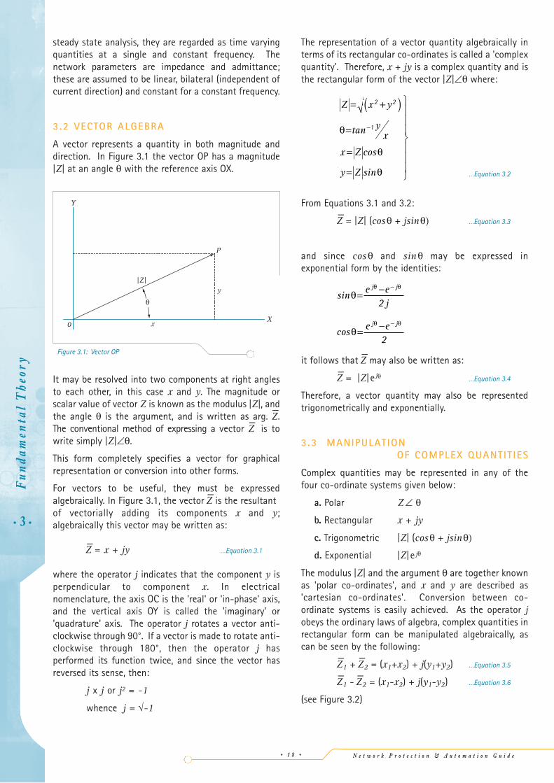
A vector represents a quantity in both magnitude anddirection. In Figure 3.1 the vector OP has a magnitude|Z| at an angle θ with the reference axis OX.
Figure 3.1
It may be resolved into two components at right anglesto each other, in this case x and y. The magnitude orscalar value of vector Z is known as the modulus |Z|, andthe angle θ is the argument, and is written as arg.
—Z.
The conventional method of expressing a vector Z—
is towrite simply |Z|∠θ.
This form completely specifies a vector for graphicalrepresentation or conversion into other forms.
For vectors to be useful, they must be expressedalgebraically. In Figure 3.1, the vector
—Z is the resultant
of vectorially adding its components x and y;algebraically this vector may be written as:
—Z = x + jy …Equation 3.1
where the operator j indicates that the component y isperpendicular to component x. In electricalnomenclature, the axis OC is the 'real' or 'in-phase' axis,and the vertical axis OY is called the 'imaginary' or'quadrature' axis. The operator j rotates a vector anti-clockwise through 90°. If a vector is made to rotate anti-clockwise through 180°, then the operator j hasperformed its function twice, and since the vector hasreversed its sense, then:
j x j or j2 = -1
whence j = √-1
The representation of a vector quantity algebraically interms of its rectangular co-ordinates is called a 'complexquantity'. Therefore, x + jy is a complex quantity and isthe rectangular form of the vector |Z|∠θ where:
—…Equation 3.2
From Equations 3.1 and 3.2:—Z = |Z| (cosθ + jsinθ) …Equation 3.3
and since cosθ and sinθ may be expressed inexponential form by the identities:
it follows that—Z may also be written as:
—Z = |Z|e jθ …Equation 3.4
Therefore, a vector quantity may also be representedtrigonometrically and exponentially.
3.3 MANIPULATIONOF COMPLEX QUANTIT IES
Complex quantities may be represented in any of thefour co-ordinate systems given below:
a. Polar Z∠ θ
b. Rectangular x + jy
c. Trigonometric |Z| (cosθ + jsinθ)
d. Exponential |Z|e jθ
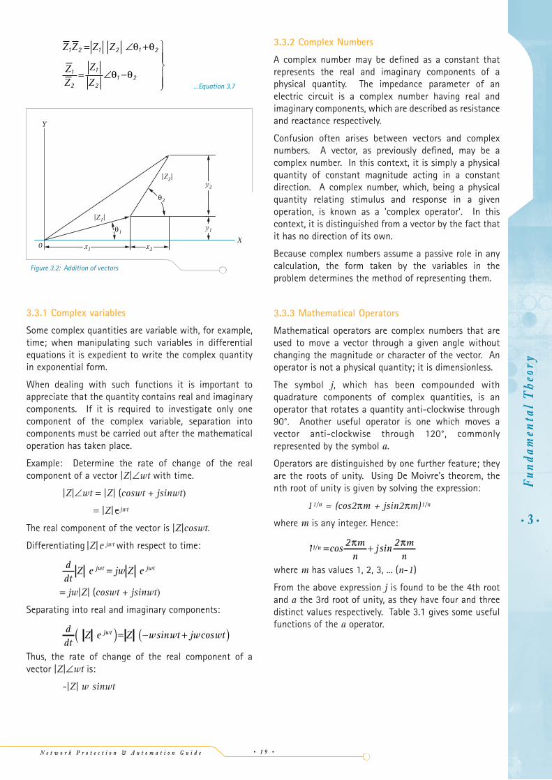
The modulus |Z| and the argument θ are together knownas 'polar co-ordinates', and x and y are described as'cartesian co-ordinates'. Conversion between co-ordinate systems is easily achieved. As the operator jobeys the ordinary laws of algebra, complex quantities inrectangular form can be manipulated algebraically, ascan be seen by the following:
—Z1 +
—Z2 = (x1+x2) + j(y1+y2) …Equation 3.5
—Z1 -
—Z2 = (x1-x2) + j(y1-y2) …Equation 3.6
(see Figure 3.2)
cosθθ θ
= − −e ej j
2
sinθθ θ
= − −e ej
j j
2
Z x y
yx
x Z
y Z
= +( )=
=
=
−
2 2
1θ
θ
θ
tan
cos
sin
Figure 3.1: Vector OPFigure 3.1: Vector OP
0
Y
X
P
|Z|y
x
q
N e t w o r k P r o t e c t i o n & A u t o m a t i o n G u i d e • 1 9 •
• 3 •F
unda
men
tal
The
ory
…Equation 3.7
3.3.1 Complex variables
Some complex quantities are variable with, for example,time; when manipulating such variables in differentialequations it is expedient to write the complex quantityin exponential form.
When dealing with such functions it is important toappreciate that the quantity contains real and imaginarycomponents. If it is required to investigate only onecomponent of the complex variable, separation intocomponents must be carried out after the mathematicaloperation has taken place.
Example: Determine the rate of change of the realcomponent of a vector |Z|∠wt with time.
|Z|∠wt = |Z| (coswt + jsinwt)
= |Z|e jwt
The real component of the vector is |Z|coswt.
Differentiating |Z|e jwt with respect to time:
= jw|Z| (coswt + jsinwt)
Separating into real and imaginary components:
Thus, the rate of change of the real component of avector |Z|∠wt is:
-|Z| w sinwt
ddt
Z e Z w wt jw wtjwt( )= − +( )sin cos
ddt
Z e jw Z ejwt jwt =
Z Z Z Z
ZZ
Z
Z
1 2 1 2 1 2
1
2
1
21 2
= ∠ +
= ∠ −
θ θ
θ θ
3.3.2 Complex Numbers
A complex number may be defined as a constant thatrepresents the real and imaginary components of aphysical quantity. The impedance parameter of anelectric circuit is a complex number having real andimaginary components, which are described as resistanceand reactance respectively.
Confusion often arises between vectors and complexnumbers. A vector, as previously defined, may be acomplex number. In this context, it is simply a physicalquantity of constant magnitude acting in a constantdirection. A complex number, which, being a physicalquantity relating stimulus and response in a givenoperation, is known as a 'complex operator'. In thiscontext, it is distinguished from a vector by the fact thatit has no direction of its own.
Because complex numbers assume a passive role in anycalculation, the form taken by the variables in theproblem determines the method of representing them.
3.3.3 Mathematical Operators
Mathematical operators are complex numbers that areused to move a vector through a given angle withoutchanging the magnitude or character of the vector. Anoperator is not a physical quantity; it is dimensionless.
The symbol j, which has been compounded withquadrature components of complex quantities, is anoperator that rotates a quantity anti-clockwise through90°. Another useful operator is one which moves avector anti-clockwise through 120°, commonlyrepresented by the symbol a.
Operators are distinguished by one further feature; theyare the roots of unity. Using De Moivre's theorem, thenth root of unity is given by solving the expression:
11/n = (cos2πm + jsin2πm)1/n
where m is any integer. Hence:
where m has values 1, 2, 3, ... (n-1)
From the above expression j is found to be the 4th rootand a the 3rd root of unity, as they have four and threedistinct values respectively. Table 3.1 gives some usefulfunctions of the a operator.
1 2 21/ cos sinn
mn
j mn
= +π π
Figure 3.2: Addition of vectorsFigure 3.2: Addition of vectors
0
Y
X
y1
y2
x2x1
|Z1|
|Z2|
N e t w o r k P r o t e c t i o n & A u t o m a t i o n G u i d e
1=1+ j0 = e j0
1+ a + a2 = 0
Table 3.1: Properties of the a operator
3.4 C IRCUIT QUANTIT IESAND CONVENTIONS
Circuit analysis may be described as the study of theresponse of a circuit to an imposed condition, forexample a short circuit. The circuit variables are currentand voltage. Conventionally, current flow results fromthe application of a driving voltage, but there iscomplete duality between the variables and either maybe regarded as the cause of the other.
When a circuit exists, there is an interchange of energy;a circuit may be described as being made up of 'sources'and 'sinks' for energy. The parts of a circuit are describedas elements; a 'source' may be regarded as an 'active'element and a 'sink' as a 'passive' element. Some circuitelements are dissipative, that is, they are continuoussinks for energy, for example resistance. Other circuitelements may be alternately sources and sinks, forexample capacitance and inductance. The elements of acircuit are connected together to form a network havingnodes (terminals or junctions) and branches (seriesgroups of elements) that form closed loops (meshes).
In steady state a.c. circuit theory, the ability of a circuitto accept a current flow resulting from a given drivingvoltage is called the impedance of the circuit. Sincecurrent and voltage are duals the impedance parametermust also have a dual, called admittance.
3.4.1 Circuit Variables
As current and voltage are sinusoidal functions of time,varying at a single and constant frequency, they areregarded as rotating vectors and can be drawn as planvectors (that is, vectors defined by two co-ordinates) ona vector diagram.
j a a= − 2
3
a a j− =2 3
1 32− =−a j a
1 3 2− =a j a
a j ej2
43
12
32
=− − =π
a j ej
=− + =12
32
23π
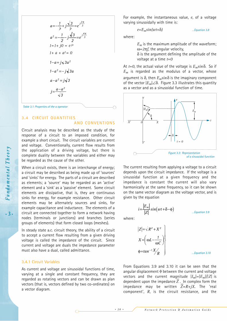
For example, the instantaneous value, e, of a voltagevarying sinusoidally with time is:
e=Emsin(wt+δ) …Equation 3.8
where:
Em is the maximum amplitude of the waveform;ω=2πf, the angular velocity, δ is the argument defining the amplitude of thevoltage at a time t=0
At t=0, the actual value of the voltage is Emsinδ. So ifEm is regarded as the modulus of a vector, whose
argument is δ, then Emsinδ is the imaginary componentof the vector |Em|∠δ. Figure 3.3 illustrates this quantityas a vector and as a sinusoidal function of time.
Figure 3.3
The current resulting from applying a voltage to a circuitdepends upon the circuit impedance. If the voltage is asinusoidal function at a given frequency and theimpedance is constant the current will also varyharmonically at the same frequency, so it can be shownon the same vector diagram as the voltage vector, and isgiven by the equation
…Equation 3.9
where:
…Equation 3.10
From Equations 3.9 and 3.10 it can be seen that theangular displacement φ between the current and voltagevectors and the current magnitude |Im|=|Em|/|Z| isdependent upon the impedance
—Z . In complex form the
impedance may be written—Z=R+jX. The 'real
component', R, is the circuit resistance, and the
Z R X
X LC
XR
= +
= −
=
−
2 2
1
1ωω
φ tan
iE
Zwtm= + −( )sin δ φ
• 3 •
Fun
dam
enta
l T
heor
y
• 2 0 •
Figure 3.3: Representationof a sinusoidal function
Figure 3.3: Representation of a sinusoidal function
Y
X' X0
Y'
e
t = 0
t
|Em| Em
N e t w o r k P r o t e c t i o n & A u t o m a t i o n G u i d e • 2 1 •
'imaginary component', X, is the circuit reactance. Whenthe circuit reactance is inductive (that is, wL>1/wC), thecurrent 'lags' the voltage by an angle φ, and when it iscapacitive (that is, 1/wC>wL) it 'leads' the voltage by anangle φ.
When drawing vector diagrams, one vector is chosen asthe 'reference vector' and all other vectors are drawnrelative to the reference vector in terms of magnitudeand angle. The circuit impedance |Z| is a complexoperator and is distinguished from a vector only by thefact that it has no direction of its own. A furtherconvention is that sinusoidally varying quantities aredescribed by their 'effective' or 'root mean square' (r.m.s.)values; these are usually written using the relevantsymbol without a suffix.
Thus:
…Equation 3.11
The 'root mean square' value is that value which has thesame heating effect as a direct current quantity of thatvalue in the same circuit, and this definition applies tonon-sinusoidal as well as sinusoidal quantities.
3.4.2 Sign Conventions
In describing the electrical state of a circuit, it is oftennecessary to refer to the 'potential difference' existingbetween two points in the circuit. Since wherever sucha potential difference exists, current will flow and energywill either be transferred or absorbed, it is obviouslynecessary to define a potential difference in more exactterms. For this reason, the terms voltage rise and voltagedrop are used to define more accurately the nature of thepotential difference.
Voltage rise is a rise in potential measured in thedirection of current flow between two points in a circuit.Voltage drop is the converse. A circuit element with avoltage rise across it acts as a source of energy. A circuitelement with a voltage drop across it acts as a sink ofenergy. Voltage sources are usually active circuitelements, while sinks are usually passive circuitelements. The positive direction of energy flow is fromsources to sinks.
Kirchhoff's first law states that the sum of the drivingvoltages must equal the sum of the passive voltages in aclosed loop. This is illustrated by the fundamentalequation of an electric circuit:
…Equation 3.12
where the terms on the left hand side of the equation arevoltage drops across the circuit elements. Expressed in
iR Ldidt C
idt e+ + =∫1
I I
E E
m
m
=
=
2
2
steady state terms Equation 3.12 may be written:
…Equation 3.13
and this is known as the equated-voltage equation [3.1].
It is the equation most usually adopted in electricalnetwork calculations, since it equates the drivingvoltages, which are known, to the passive voltages,which are functions of the currents to be calculated.
In describing circuits and drawing vector diagrams, forformal analysis or calculations, it is necessary to adopt anotation which defines the positive direction of assumedcurrent flow, and establishes the direction in whichpositive voltage drops and voltage rises act. Twomethods are available; one, the double suffix method, isused for symbolic analysis, the other, the single suffix ordiagrammatic method, is used for numericalcalculations.
In the double suffix method the positive direction ofcurrent flow is assumed to be from node a to node b andthe current is designated Iab . With the diagrammaticmethod, an arrow indicates the direction of current flow.
The voltage rises are positive when acting in thedirection of current flow. It can be seen from Figure 3.4that
—E1 and
—Ean are positive voltage rises and
—E2 and—
Ebn are negative voltage rises. In the diagrammaticmethod their direction of action is simply indicated by anarrow, whereas in the double suffix method,
—Ean and
—Ebn
indicate that there is a potential rise in directions na and nb.
Figure 3.4 Methods or representing a circuit
E IZ∑ ∑=
• 3 •F
unda
men
tal
The
ory
(a) Diagrammatic
Figure 3.4: Circuit representation methods
(b) Double suffix
a b
n
abI
Z3
Z2Z1
E1
Zan
Zab
Ean
Zbn
Ebn
E2
E1-E2=(Z1+Z2+Z3)I
Ean-Ebn=(Zan+Zab+Zbn)Iab
I
Figure 3.4 Methods of representing a circuit
N e t w o r k P r o t e c t i o n & A u t o m a t i o n G u i d e
Voltage drops are also positive when acting in thedirection of current flow. From Figure 3.4(a) it can beseen that (
—Z1+
—Z2+
—Z3)
—I is the total voltage drop in the
loop in the direction of current flow, and must equate tothe total voltage rise
—E1-
—E2. In Figure 3.4(b), the voltage
drop between nodes a and b designated —Vab indicates
that point b is at a lower potential than a, and is positivewhen current flows from a to b. Conversely
—Vba is a
negative voltage drop.
Symbolically:—Vab =
—Van -
—Vbn
—Vba =
—Vbn -
—Van …Equation 3.14
where n is a common reference point.
3.4.3 Power
The product of the potential difference across and thecurrent through a branch of a circuit is a measure of therate at which energy is exchanged between that branchand the remainder of the circuit. If the potentialdifference is a positive voltage drop, the branch ispassive and absorbs energy. Conversely, if the potentialdifference is a positive voltage rise, the branch is activeand supplies energy.
The rate at which energy is exchanged is known aspower, and by convention, the power is positive whenenergy is being absorbed and negative when beingsupplied. With a.c. circuits the power alternates, so, toobtain a rate at which energy is supplied or absorbed, itis necessary to take the average power over one wholecycle.If e=Emsin(wt+δ) and i=Imsin(wt+δ-φ), then the powerequation is:
p=ei=P[1-cos2(wt+δ)]+Qsin2(wt+δ)
…Equation 3.15where:
P=|E||I|cosφ and
Q=|E||I|sinφ
From Equation 3.15 it can be seen that the quantity Pvaries from 0 to 2P and quantity Q varies from -Q to +Qin one cycle, and that the waveform is of twice theperiodic frequency of the current voltage waveform.
The average value of the power exchanged in one cycleis a constant, equal to quantity P, and as this quantity isthe product of the voltage and the component of currentwhich is 'in phase' with the voltage it is known as the'real' or 'active' power.
The average value of quantity Q is zero when taken overa cycle, suggesting that energy is stored in one half-cycleand returned to the circuit in the remaining half-cycle.Q is the product of voltage and the quadrature
ab an bn
ba bn an
V V V
V V V
= −
= −
component of current, and is known as 'reactive power'.
As P and Q are constants which specify the powerexchange in a given circuit, and are products of thecurrent and voltage vectors, then if
—S is the vector
product —E
—I it follows that with
—E as the reference vector
and φ as the angle between—E and
—I :
—S = P + jQ …Equation 3.16
The quantity—S is described as the 'apparent power', and
is the term used in establishing the rating of a circuit.—S has units of VA.
3.4.4 Single-Phase and Polyphase Systems
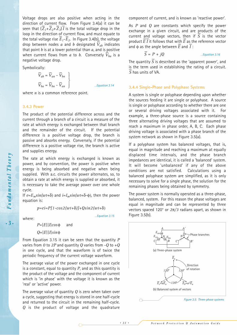
A system is single or polyphase depending upon whetherthe sources feeding it are single or polyphase. A sourceis single or polyphase according to whether there are oneor several driving voltages associated with it. Forexample, a three-phase source is a source containingthree alternating driving voltages that are assumed toreach a maximum in phase order, A, B, C. Each phasedriving voltage is associated with a phase branch of thesystem network as shown in Figure 3.5(a).
If a polyphase system has balanced voltages, that is,equal in magnitude and reaching a maximum at equallydisplaced time intervals, and the phase branchimpedances are identical, it is called a 'balanced' system.It will become 'unbalanced' if any of the aboveconditions are not satisfied. Calculations using abalanced polyphase system are simplified, as it is onlynecessary to solve for a single phase, the solution for theremaining phases being obtained by symmetry.
The power system is normally operated as a three-phase,balanced, system. For this reason the phase voltages areequal in magnitude and can be represented by threevectors spaced 120° or 2π/3 radians apart, as shown inFigure 3.5(b).
• 3 •
Fun
dam
enta
l T
heor
y
• 2 2 •
Figure 3.5: Three-phase systems
(a) Three-phase system
Figure 3.5: Three-phase systems
BC B'C'N N'
EanEcn Ebn
A'A
Phase branches
Direction of rotation
(b) Balanced system of vectors
120°
120°
120°
Ea
Ec=aEa Eb=a2Ea
N e t w o r k P r o t e c t i o n & A u t o m a t i o n G u i d e • 2 3 •
Since the voltages are symmetrical, they may beexpressed in terms of one, that is:
—Ea =
—Ea
—Eb = a2
—Ea
—Ec = a
—Ea …Equation 3.17
where a is the vector operator e j2π/3. Further, if the phasebranch impedances are identical in a balanced system, itfollows that the resulting currents are also balanced.
3.5 IMPEDANCE NOTATION
It can be seen by inspection of any power systemdiagram that:
a. several voltage levels exist in a system
b. it is common practice to refer to plant MVA interms of per unit or percentage values
c. transmission line and cable constants are given inohms/km
Before any system calculations can take place, thesystem parameters must be referred to 'base quantities'and represented as a unified system of impedances ineither ohmic, percentage, or per unit values.
The base quantities are power and voltage. Normally,they are given in terms of the three-phase power in MVAand the line voltage in kV. The base impedance resultingfrom the above base quantities is:
ohms …Equation 3.18
and, provided the system is balanced, the baseimpedance may be calculated using either single-phaseor three-phase quantities.
The per unit or percentage value of any impedance in thesystem is the ratio of actual to base impedance values.
Hence:
…Equation 3.19
where MVAb = base MVA
kVb = base kV
Simple transposition of the above formulae will refer theohmic value of impedance to the per unit or percentagevalues and base quantities.
Having chosen base quantities of suitable magnitude all
Z p u Z ohms MVA
kV
Z Z p u
b
b
. .
% . .
( )= ( )×( )
( )= ( )×
2
100
ZkV
MVAb =( )2
a a
b a
c a
E E
E E
E E
a
a
=
=
=
2
system impedances may be converted to those basequantities by using the equations given below:
…Equation 3.20
where suffix b1 denotes the value to the original base
and b2 denotes the value to new base
The choice of impedance notation depends upon thecomplexity of the system, plant impedance notation andthe nature of the system calculations envisaged.
If the system is relatively simple and contains mainlytransmission line data, given in ohms, then the ohmicmethod can be adopted with advantage. However, theper unit method of impedance notation is the mostcommon for general system studies since:
1. impedances are the same referred to either side ofa transformer if the ratio of base voltages on thetwo sides of a transformer is equal to thetransformer turns ratio
2. confusion caused by the introduction of powers of100 in percentage calculations is avoided
3. by a suitable choice of bases, the magnitudes ofthe data and results are kept within a predictablerange, and hence errors in data and computationsare easier to spot
Most power system studies are carried out usingsoftware in per unit quantities. Irrespective of themethod of calculation, the choice of base voltage, andunifying system impedances to this base, should beapproached with caution, as shown in the followingexample.
Z Z MVAMVA
Z Z kVkV
b bb
b
b bb
b
2 12
1
2 11
2
2
= ×
= ×
• 3 •F
unda
men
tal
The
ory
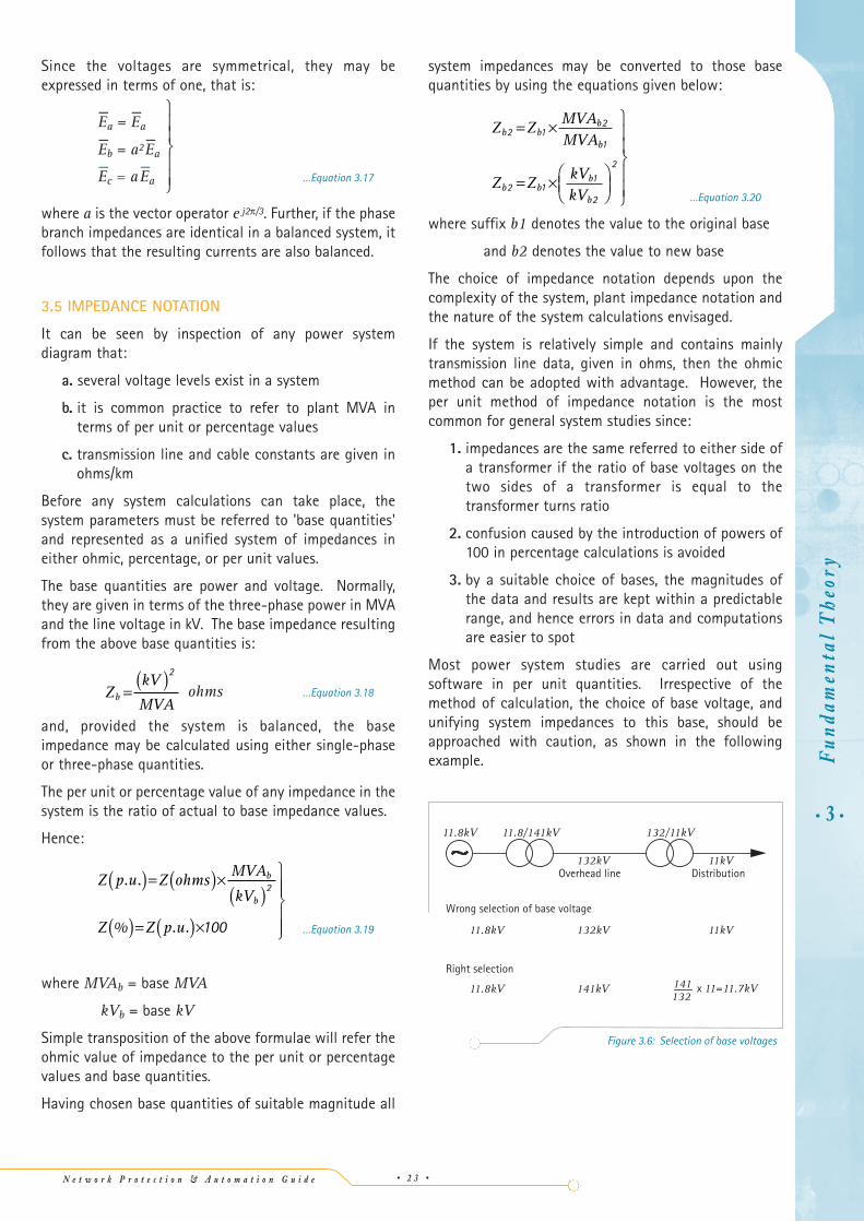
Figure 3.6: Selection of base voltages
Figure 3.6: Selection of base voltages
11.8kV 11.8/141kV
132kVOverhead line
132/11kV
Distribution11kV
Wrong selection of base voltage
11.8kV 132kV 11kV
Right selection
11.8kV 141kV x 11=11.7kV141132
N e t w o r k P r o t e c t i o n & A u t o m a t i o n G u i d e
From Figure 3.6 it can be seen that the base voltages inthe three circuits are related by the turns ratios of theintervening transformers. Care is required as thenominal transformation ratios of the transformersquoted may be different from the turns ratios- e.g. a110/33kV (nominal) transformer may have a turns ratioof 110/34.5kV. Therefore, the rule for hand calculationsis: 'to refer an impedance in ohms from one circuit toanother multiply the given impedance by the square ofthe turns ratio (open circuit voltage ratio) of theintervening transformer'.
Where power system simulation software is used, thesoftware normally has calculation routines built in toadjust transformer parameters to take account ofdifferences between the nominal primary and secondaryvoltages and turns ratios. In this case, the choice of basevoltages may be more conveniently made as the nominalvoltages of each section of the power system. Thisapproach avoids confusion when per unit or percentvalues are used in calculations in translating the finalresults into volts, amps, etc.
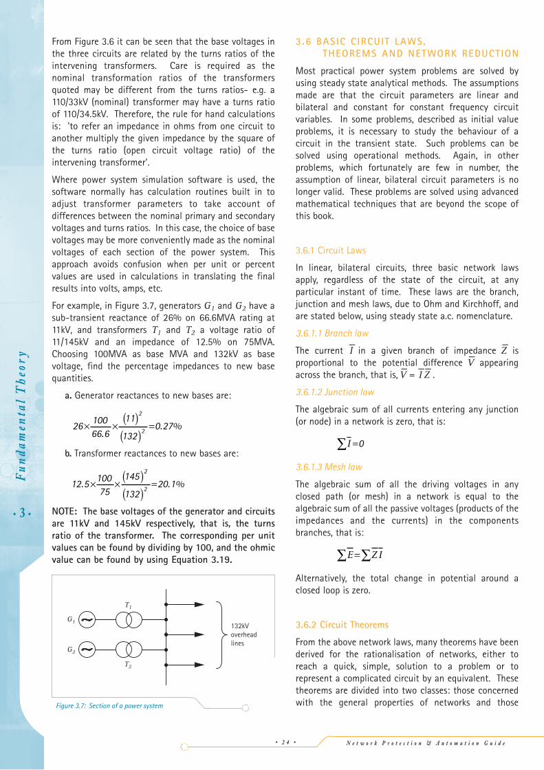
For example, in Figure 3.7, generators G1 and G2 have asub-transient reactance of 26% on 66.6MVA rating at11kV, and transformers T1 and T2 a voltage ratio of11/145kV and an impedance of 12.5% on 75MVA.Choosing 100MVA as base MVA and 132kV as basevoltage, find the percentage impedances to new basequantities.
a. Generator reactances to new bases are:
b. Transformer reactances to new bases are:
NOTE: The base voltages of the generator and circuitsare 11kV and 145kV respectively, that is, the turnsratio of the transformer. The corresponding per unitvalues can be found by dividing by 100, and the ohmicvalue can be found by using Equation 3.19.
Figure 3.7
12 5 10075
145
13220 1
2
2. . %× ×( )( )
=
26 10066 6
11
1320 27
2
2× ×( )
( )=
.. %
3.6 BASIC CIRCUIT LAWS,THEOREMS AND NETWORK REDUCTION
Most practical power system problems are solved byusing steady state analytical methods. The assumptionsmade are that the circuit parameters are linear andbilateral and constant for constant frequency circuitvariables. In some problems, described as initial valueproblems, it is necessary to study the behaviour of acircuit in the transient state. Such problems can besolved using operational methods. Again, in otherproblems, which fortunately are few in number, theassumption of linear, bilateral circuit parameters is nolonger valid. These problems are solved using advancedmathematical techniques that are beyond the scope ofthis book.
3.6.1 Circuit Laws
In linear, bilateral circuits, three basic network lawsapply, regardless of the state of the circuit, at anyparticular instant of time. These laws are the branch,junction and mesh laws, due to Ohm and Kirchhoff, andare stated below, using steady state a.c. nomenclature.
3.6.1.1 Branch law
The current—I in a given branch of impedance
—Z is
proportional to the potential difference—V appearing
across the branch, that is,—V =
—I
—Z .
3.6.1.2 Junction law
The algebraic sum of all currents entering any junction(or node) in a network is zero, that is:
3.6.1.3 Mesh law
The algebraic sum of all the driving voltages in anyclosed path (or mesh) in a network is equal to thealgebraic sum of all the passive voltages (products of theimpedances and the currents) in the componentsbranches, that is:
Alternatively, the total change in potential around aclosed loop is zero.
3.6.2 Circuit Theorems
From the above network laws, many theorems have beenderived for the rationalisation of networks, either toreach a quick, simple, solution to a problem or torepresent a complicated circuit by an equivalent. Thesetheorems are divided into two classes: those concernedwith the general properties of networks and those
E ZI=∑∑
I =∑ 0
• 3 •
Fun
dam
enta
l T
heor
y
• 2 4 •
Figure 3.7: Section of a power system
Figure 3.7: Section of a power system
G1
T1
T2
G2
132kVoverheadlines
N e t w o r k P r o t e c t i o n & A u t o m a t i o n G u i d e • 2 5 •
concerned with network reduction.
Of the many theorems that exist, the three mostimportant are given. These are: the SuperpositionTheorem, Thévenin's Theorem and Kennelly's Star/DeltaTheorem.
3.6.2.1 Superposition Theorem(general network theorem)
The resultant current that flows in any branch of anetwork due to the simultaneous action of severaldriving voltages is equal to the algebraic sum of thecomponent currents due to each driving voltage actingalone with the remainder short-circuited.
3.6.2.2 Thévenin's Theorem(active network reduction theorem)
Any active network that may be viewed from twoterminals can be replaced by a single driving voltageacting in series with a single impedance. The drivingvoltage is the open-circuit voltage between the twoterminals and the impedance is the impedance of thenetwork viewed from the terminals with all sourcesshort-circuited.
3.6.2.3 Kennelly's Star/Delta Theorem(passive network reduction theorem)
Any three-terminal network can be replaced by a delta orstar impedance equivalent without disturbing theexternal network. The formulae relating the replacementof a delta network by the equivalent star network is asfollows (Figure 3.8):
—Zco =
—Z13
—Z23 / (
—Z12 +
—Z13 +
—Z23)
and so on.
Figure 3.8: Star/Delta network reduction
The impedance of a delta network corresponding to andreplacing any star network is:
—Z12 = —Zao +
—Zbo +—Zao
—Zbo
—————————Zco
and so on.
3.6.3 Network Reduction
The aim of network reduction is to reduce a system to asimple equivalent while retaining the identity of thatpart of the system to be studied.
For example, consider the system shown in Figure 3.9.The network has two sources E ’ and E ’’, a line AOBshunted by an impedance, which may be regarded as thereduction of a further network connected between A andB, and a load connected between O and N. The object ofthe reduction is to study the effect of opening a breakerat A or B during normal system operations, or of a faultat A or B. Thus the identity of nodes A and B must beretained together with the sources, but the branch ONcan be eliminated, simplifying the study. Proceeding, A,B, N, forms a star branch and can therefore be convertedto an equivalent delta.
Figure 3.9
= 51 ohms
=30.6 ohms
= 1.2 ohms (since ZNO>>> ZAOZBO)
Figure 3.10
Z Z Z Z ZZAN AO BOAO BO
NO
= + +
= + + ×0 45 18 85 0 45 18 850 75
. . . ..
Z Z Z Z ZZBN BO NOBO NO
AO
= + +
= + + ×0 75 18 85 0 75 18 850 45
. . . ..
Z Z Z Z ZZAN AO NOAO NO
BO
= + +
• 3 •F
unda
men
tal
The
ory
Figure 3.8: Star-Delta network transformationFigure 3.8: Star-Delta network transformation
c
Zao Zbo Z12
Z23Z13
Oa b 1 2
3
(a) Star network (b) Delta network
Zco
Figure 3.9: Typical power system networkFigure 3.9: Typical power system network
E' E''
N
0A B
1.6Ω
0.75Ω 0.45Ω
18.85Ω
2.55Ω
0.4Ω
N e t w o r k P r o t e c t i o n & A u t o m a t i o n G u i d e
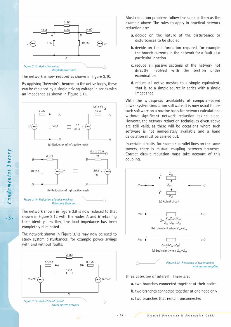
The network is now reduced as shown in Figure 3.10.
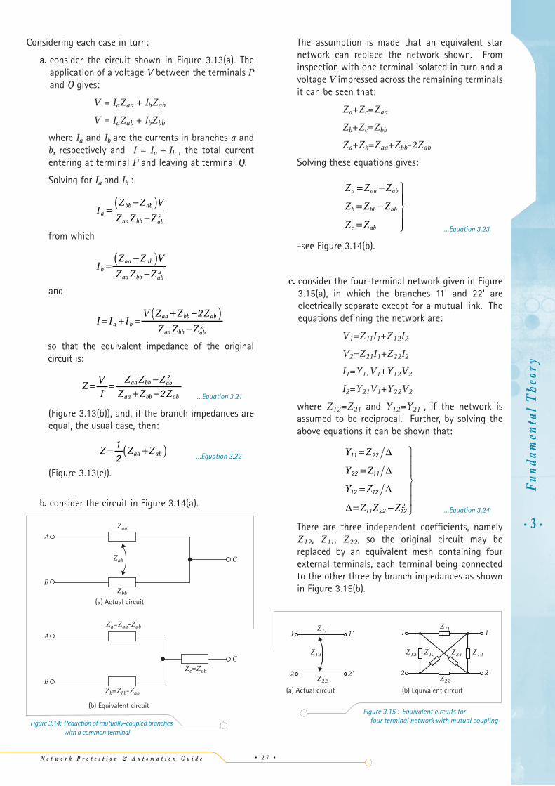
By applying Thévenin's theorem to the active loops, thesecan be replaced by a single driving voltage in series withan impedance as shown in Figure 3.11.
Figure 3.11
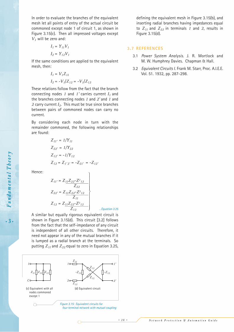
The network shown in Figure 3.9 is now reduced to thatshown in Figure 3.12 with the nodes A and B retainingtheir identity. Further, the load impedance has beencompletely eliminated.
The network shown in Figure 3.12 may now be used tostudy system disturbances, for example power swingswith and without faults.
Figure 3.12
Most reduction problems follow the same pattern as theexample above. The rules to apply in practical networkreduction are:
a. decide on the nature of the disturbance ordisturbances to be studied
b. decide on the information required, for examplethe branch currents in the network for a fault at aparticular location
c. reduce all passive sections of the network notdirectly involved with the section underexamination
d. reduce all active meshes to a simple equivalent,that is, to a simple source in series with a singleimpedance
With the widespread availability of computer-basedpower system simulation software, it is now usual to usesuch software on a routine basis for network calculationswithout significant network reduction taking place.However, the network reduction techniques given aboveare still valid, as there will be occasions where suchsoftware is not immediately available and a handcalculation must be carried out.
In certain circuits, for example parallel lines on the sametowers, there is mutual coupling between branches.Correct circuit reduction must take account of thiscoupling.
Figure 3.13
Three cases are of interest. These are:
a. two branches connected together at their nodes
b. two branches connected together at one node only
c. two branches that remain unconnected
• 3 •
Fun
dam
enta
l T
heor
y
• 2 6 •
Figure 3.10: Reduction usingstar/delta transform
E'
A
51Ω 30.6Ω
0.4Ω
2.5Ω
1.2Ω1.6Ω
N
B
E''
Figure 3.12: Reduction of typicalpower system network
Figure 3.12: Reduction of typical power system network
N
A B
1.2Ω
2.5Ω
1.55Ω
0.97E'
0.39Ω
0.99E''
Figure 3.11: Reduction of active meshes: Thévenin's Theorem
Figure 3.11: Reduction of active meshes: Thévenin's Theorem
E'
A
N
(a) Reduction of left active mesh
N
A
(b) Reduction of right active mesh
E''
N
B B
N
E''31
30.630.6Ω
Ω31
0.4 x 30.6
Ω52.6
1.6 x 51
E'52.65151Ω
1.6Ω
0.4Ω
Figure 3.13: Reduction of two brancheswith mutual couplingFigure 3.13: Reduction of two branches with mutual coupling
(a) Actual circuit
IP Q
P Q
(b) Equivalent when Zaa≠Zbb
(c) Equivalent when Zaa=Zbb
P Q
21Z= (Zaa+Zbb)
Zaa
Zbb
Z=ZaaZbb-Z2
ab
Zaa+Zbb-2Zab
Zab
Ia
Ib
I
I
N e t w o r k P r o t e c t i o n & A u t o m a t i o n G u i d e • 2 7 •
Considering each case in turn:
a. consider the circuit shown in Figure 3.13(a). Theapplication of a voltage V between the terminals Pand Q gives:
V = IaZaa + IbZab
V = IaZab + IbZbb
where Ia and Ib are the currents in branches a andb, respectively and I = Ia + Ib , the total currententering at terminal P and leaving at terminal Q.
Solving for Ia and Ib :
from which
and
so that the equivalent impedance of the originalcircuit is:
…Equation 3.21
(Figure 3.13(b)), and, if the branch impedances areequal, the usual case, then:
…Equation 3.22
(Figure 3.13(c)).
b. consider the circuit in Figure 3.14(a).
Z Z Zaa ab= +( )12
Z VI
Z Z ZZ Z Z
aa bb ab
aa bb ab
= = −+ −
2
2
I I IV Z Z Z
Z Z Za baa bb ab
aa bb ab
= + =+ −( )
−22
IZ Z V
Z Z Zbaa ab
aa bb ab
=−( )
− 2
IZ Z V
Z Z Zabb ab
aa bb ab
=−( )
− 2
The assumption is made that an equivalent starnetwork can replace the network shown. Frominspection with one terminal isolated in turn and avoltage V impressed across the remaining terminalsit can be seen that:
Za+Zc=Zaa
Zb+Zc=Zbb
Za+Zb=Zaa+Zbb-2Zab
Solving these equations gives:
…Equation 3.23
-see Figure 3.14(b).
c. consider the four-terminal network given in Figure3.15(a), in which the branches 11' and 22' areelectrically separate except for a mutual link. Theequations defining the network are:
V1=Z11I1+Z12I2
V2=Z21I1+Z22I2
I1=Y11V1+Y12V2
I2=Y21V1+Y22V2
where Z12=Z21 and Y12=Y21 , if the network isassumed to be reciprocal. Further, by solving theabove equations it can be shown that:
…Equation 3.24
There are three independent coefficients, namelyZ12, Z11, Z22, so the original circuit may bereplaced by an equivalent mesh containing fourexternal terminals, each terminal being connectedto the other three by branch impedances as shownin Figure 3.15(b).
Y Z
Y Z
Y Z
Z Z Z
11 22
22 11
12 12
11 22 122
=
=
=
= −
∆
∆
∆
∆
Z Z Z
Z Z Z
Z Z
a aa ab
b bb ab
c ab
= −
= −
=
• 3 •F
unda
men
tal
The
ory
Figure 3.14: Reduction of mutually-coupled brancheswith a common terminal
A
C
B
(b) Equivalent circuit
B
C
A
Figure 3.14: Reduction of mutually-coupled branches with a common terminal
(a) Actual circuit
Zaa
Zbb
Zab
Za=Zaa-Zab
Zb=Zbb-Zab
Zc=Zab
Figure 3.15 : Equivalent circuits forfour terminal network with mutual coupling
(a) Actual circuit
2
1
2'
1'
2'
1'
2'
1'
(b) Equivalent circuit
(d) Equivalent circuit
2
1
11
C 2
(c) Equivalent with all nodes commoned
Z11
Z11 Z12
Z22
Z11
Z11
Z12
Z12
Z12
-Z12 -Z12
Z22
Z12
Z12
Z12 Z12 Z12Z21
N e t w o r k P r o t e c t i o n & A u t o m a t i o n G u i d e
defining the equivalent mesh in Figure 3.15(b), andinserting radial branches having impedances equalto Z11 and Z22 in terminals 1 and 2, results inFigure 3.15(d).
3.7 REFERENCES
3.1 Power System Analysis. J. R. Mortlock andM. W. Humphrey Davies. Chapman & Hall.
3.2 Equivalent Circuits I. Frank M. Starr, Proc. A.I.E.E.Vol. 51. 1932, pp. 287-298.
• 3 •
Fun
dam
enta
l T
heor
y
• 2 8 •
Figure 3.15: Equivalent circuits forfour terminal network with mutual coupling
Figure 3.15: Equivalent circuits for four terminal network with mutual coupling
(a) Actual circuit
2
1
2'
1'
2'
1'
2'
1'
(b) Equivalent circuit
(d) Equivalent circuit
2
1
11
C 2
(c) Equivalent with all nodes commoned except 1
Z11
Z11 Z12
Z22
Z11
Z11
Z12
Z12
Z12
-Z12 -Z12
Z22
Z12
Z12
Z12 Z12 Z12Z21
In order to evaluate the branches of the equivalentmesh let all points of entry of the actual circuit becommoned except node 1 of circuit 1, as shown inFigure 3.15(c). Then all impressed voltages exceptV1 will be zero and:
I1 = Y11V1
I2 = Y12V1
If the same conditions are applied to the equivalentmesh, then:
I1 = V1Z11
I2 = -V1/Z12 = -V1/Z12
These relations follow from the fact that the branchconnecting nodes 1 and 1' carries current I1 andthe branches connecting nodes 1 and 2' and 1 and2 carry current I2. This must be true since branchesbetween pairs of commoned nodes can carry nocurrent.
By considering each node in turn with theremainder commoned, the following relationshipsare found:
Z11’ = 1/Y11
Z22’ = 1/Y22
Z12’ = -1/Y12
Z12 = Z1’ 2’ = -Z21’ = -Z12’
Hence:
Z11’ = Z11Z22-Z212_______________Z22
Z22’ = Z11Z22-Z212_______________Z11
Z12 = Z11Z22-Z212_______________Z12 …Equation 3.25
A similar but equally rigorous equivalent circuit isshown in Figure 3.15(d). This circuit [3.2] followsfrom the fact that the self-impedance of any circuitis independent of all other circuits. Therefore, itneed not appear in any of the mutual branches if itis lumped as a radial branch at the terminals. Soputting Z11 and Z22 equal to zero in Equation 3.25,
ZZ Z Z
Z
ZZ Z Z
Z
ZZ Z Z
Z
1111 22 12
2
22
2211 22 12
2
11
1211 22 12
2
12
'
'
= −
= −
= −


![SCISCITATOR 2015 · [1]. Riverine communities experience two main types of disturbances: natural disturbances and anthropogenic disturbances. Natural disturbances in riverine ecosystems](https://img.pdfslide.us/doc/110x75/5f27dd3959f0c41da22eeec5/sciscitator-1-riverine-communities-experience-two-main-types-of-disturbances.jpg)