38

3. Finite Element Model

A numerically approximated description of the thermal behavior of the thermopile must be

formulated due to the complexity of the geometry; no closed form analytical solution is available.

We chose the finite element method over the finite difference method to conduct this study because

of the trapezoidal profile of the detector. It would have been difficult to accurately model the

triangular edge with the rectangular grid required of the finite difference method. Using the

commercial product ALGOR, we are able to treat both the steady-state and the transient aspects of

the analysis. For consistency, some of the finite element results have been checked with a

combination of two other commercial finite element commercial packages PATRAN and ABAQUS.

3.1 Finite Element Formulation

The finite element method was originally developed for structural analysis, and it has since

been adapted to the field of heat transfer analysis. The objective is to find an approximate solution

of a given boundary-value problem. The basis of this method is the representation of the region of

calculation by finite subdivisions (subvolumes), where a spaced grid of nodes replaces a conduction

region. These nodes are the location where the solution is computed. The finite subdivisions are

called finite elements and they can have different shapes, thus giving more flexibility to the method

compared to the finite difference method. The collection of finite elements and nodes is called a

finite element mesh. Continuous variables such as temperature can be represented over the finite

element by a linear combination of polynomials called interpolation functions. These functions

39

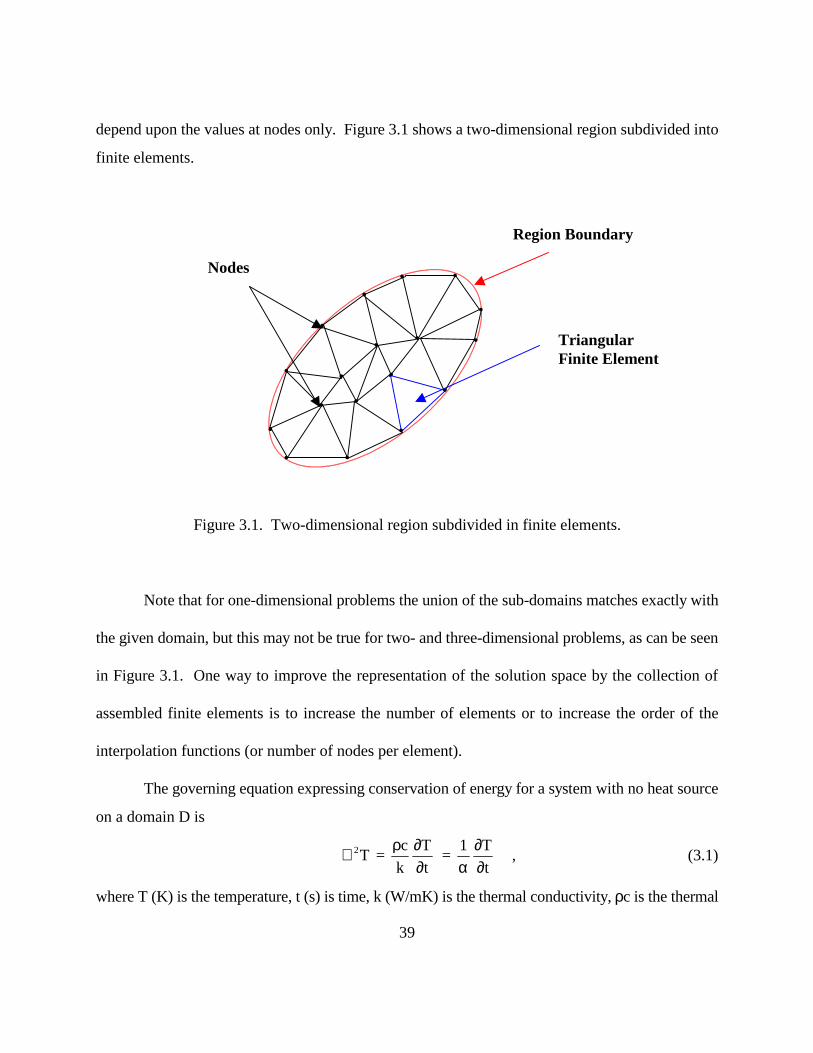
depend upon the values at nodes only. Figure 3.1 shows a two-dimensional region subdivided into

finite elements.

Figure 3.1. Two-dimensional region subdivided in finite elements.

Note that for one-dimensional problems the union of the sub-domains matches exactly with

the given domain, but this may not be true for two- and three-dimensional problems, as can be seen

in Figure 3.1. One way to improve the representation of the solution space by the collection of

assembled finite elements is to increase the number of elements or to increase the order of the

interpolation functions (or number of nodes per element).

The governing equation expressing conservation of energy for a system with no heat source

on a domain D is

, t

T

1 =

t

T

k

c = T 2

∂∂

α∂∂ρ∇ (3.1)

where T (K) is the temperature, t (s) is time, k (W/mK) is the thermal conductivity, ρc is the thermal

•

•

• •

•

•

•

• •

•

•

•

•

•• •

•

Region Boundary

Nodes

TriangularFinite Element

•

40

capacity (J/m3K) and c

k = ρ

α (m2/s) is the thermal diffusivity.

Boundary conditions such as temperature or imposed surface heat flux, including the

adiabatic condition, may be imposed on domain D. Figure 3.2 depicts these three types of boundary

conditions. In the figure, the sub-area S1 has a constant temperature boundary condition applied, S2

a constant heat flux, and S3 is insulated.

Figure 3.2. The types of available boundary conditions in ALGOR

A classical solution of the problem (strong formulation) is a function T defined on D, such

that T satisfies the given differential equation, Equation 3.1, everywhere in D and the temperature

boundary conditions. The finite element solution of the problem is based on the Galerkin

approximation which uses interpolation functions defined on the different subdivisions of the

domain D. The resulting formulation gives a system of algebraic equations to be solved. Several

methods of integration can be used to solve these equations. In transient problems, the global

formulation provides a set of equations for determining the time dependence, and calculations are

T1 imposed onsurface S1

Q´´ imposed onsurface S2

Q’’ = 0imposed onsurface S3

41

then made possible using an initial condition. For steady-state analysis one set of spatial conditions

represents the solution. Details about finite element formulation can be found in Gebhart [1993] and

Reddy [1993].

3.2 Finite Element Software

The finite element commercial package ALGOR is used to predict the response of the

thermopile radiation detector to different boundary and initial conditions. This section focuses on

the software itself, its basic operation modes, its capabilities and the numerical integration method

it uses.

3.2.1 ALGOR operation modes

ALGOR is used as the pre-processing, processing and post-processing software. First, it

prepares the model for the analysis. After having specified the nature of the analysis as either steady-

state or transient, ALGOR enables one to build the geometry, define the physical properties, and

specify the boundary conditions such as a fixed temperature, or a surface with radiation, convection

or insulation. The definition of the different material properties is made possible by assigning a

different color to each different type of material. It must also be noted that the heat flux boundary

condition is applied manually (node by node) during the pre-processing stage. ALGOR also

provides the mesh of the model by meshing the different regions into finite numbers of nodal

elements. Two-dimensional thermal elements are 3- or 4-node elements formulated in the Y-Z

plane. Meshes can be uniform across the model or concentrated around critical regions. ALGOR

also displays and verifies all data prior to executing the analysis. The pre-processing (including the

decoder and the feature called Timeload Program) is accomplished by specifying the transient

parameters, the heat flux boundary conditions and the format of the solution. The decoder then

creates a file called Filename which is the processor input file. The transient heat transfer processor

(SSAP11) processes the model.

The processor ALGOR performs the analysis by solving the system of algebraic equations

representing the model and providing an output file with the nodal results called Filename.l. The

42

post-processor displays the nodal results. Unfortunately the transient solution could not be displayed

in the desired format, and so a program was developed in Matlab which reads the nodal file,

performs different kinds of calculations (averages and errors), and plots the transient solution.

Figure 3.3summarizes the different stages used to create the model and display the results.

43

Figure 3.3. Summary of stages used in ALGOR

superdraw: Creates and editsthe model

MeshBoundary conditionsMaterial properties (colors)

Filename.esd

superview:Visualizes the model

Filename.sstNode numbers where the heatflux boundary condition must beapplied

Pre-processor

Result file nameFilename.l

Transient parametersHeat flux

Processor

Post-processor : Viewanalysis results

Instantaneous temperaturedistribution

Matlab program

Transient solution

44

3.2.2 Capabilities of and comments on the software

Comments and criticisms made below about ALGOR are usually made in comparison with

the finite element software package PATRAN (Version 2-5).

ALGOR allowed the development of a well-defined finite element mesh in the model. A

model made of 3677 elements and 3901 nodes has been created in two dimensions. Element lengths

of less than a 1 µm exist in the critical regions such as the active junction of the thermopile. The

elements used in the analysis are two-dimensional, second-order, four-node quadrilateral elements

specific to heat conduction. Since these elements are second-order, their interpolation functions are

quadratic. Quadratic functions are justified over higher-order polynomials since the mesh density

is high. Figure 3.4 shows the refined two-dimensional mesh of the part of the thermocouple

including the active junction obtained using ALGOR. Comparison of Figure 3.4 with Figure 2.8

clearly established the location of the mesh with respect to the detector geometry. This mesh is

acceptable since the elements are undistorted rectangular shaped.

Figure 3.4. Example of a two-dimensional mesh created on ALGOR.

45

The ALGOR transient thermal processor was used to perform the transient heat transfer

analysis. It is a very flexible tool in that, though it does not automatically select the time increment

so that steady state is reached, the user may define his own time increment and, even more important,

the number of steps used (up to a thousand). The drawback is that a study of the value of the time

step must first be made to know when the converged solution is reached. If this step could be made

automatic the engineering cost of the analysis would be reduced because the converged solution

would be found in a minimum number of iterations. The time integration used by ALGOR is done

with an unconditionally converging scheme called Wilson Theta. More details on this analysis can

be found in the ALGOR manual [1993].

Several other limitations of the software can be mentioned after using it and comparing it

with PATRAN. For example, the default elements are quadrilateral elements and there is no way

to use triangular elements with total control of their length or number. Another drawback of

ALGOR compared to PATRAN is the fact that the heat flux boundary conditions have to be

specified manually. When a model has a complex geometry, a boundary edge may not be numbered

sequentially and thus it becomes tedious to enter the node numbers one by one to apply the heat flux

boundary condition. Additionally an incorrect node number may be entered by mistake with the

result that the data must be entered all over again. Finally, the post-processor ALGOR is really not

flexible for displaying results. For example, it is unable to display the transient temperature response

of a specified node or group of nodes.

3.3 The Thermal Models

This section examines two thermal models, a one-dimensional model and a two-dimensional

model of the thermocouple junction pair. The assumptions and approximations implied when using

such models are given. Additionally both models are validated by presenting the results of the

derivation of an analytical steady-state solution for the one-dimensional model, and by showing that

46

the results given by another finite element software package (PATRAN-ABAQUS) confirm the two-

dimensional model.

3.3.1 General assumptions and approximations

Due to the thermopile environment (vacuum), conduction and radiation are the only modes

of heat transfer present in the analysis. Because the cavity and the heat sink where the detector is

mounted are assumed to be maintained at a temperature of 311 K, we expect the heat transfer

through radiation, other than that due to the incident heat flux from the scene, to be small, and thus

negligible in the current analysis.

Due to the high input impedance of the amplifier used to sense the thermopile voltage, we

assume that no current flows through the thermocouple junctions. Thus no self-heating nor other

thermoelectric effects are taken into account and the volumetric heat source q´´´ is assigned a value

of 0 W/m3 in the energy equation.

Since only small ranges of temperatures are encountered, it is assumed that material

properties such as conductivity do not vary with temperature.

As far as the boundary conditions are concerned, the heat sink is modeled by a fixed, known

temperature at the interface of the pixel with the aluminum-nitride substrate. This condition gives

the substrate the property of a heat sink. Assuming that the incident scene energy striking the

absorber is uniform, it is modeled as a net uniformly distributed heat flux boundary condition. This

imposed heat flux is assumed normal to the top of the pixel (the absorber). It represents the incident

radiation coming from the Earth less the component emitted from the surface of the pixel.

The gap between adjacent pixels is assumed to thermally insulate each thermocouple

junction pair of the linear-array; thus the two edges of the pixel are insulated. Since it is not yet clear

what kind of conditions exist on to the remaining boundaries of the pixel; it is assumed that they are

also insulated. This is a least partially justified because the pixel array is embedded in the cavity

mirror wall. Figure 3.5 summarizes the boundary conditions applied to the pixel.

47

Figure 3.5. Boundary conditions applied to the pixel

The pixel design shown in Figure 3.5 is geometrically three-dimensional. However, the

symmetry in the boundary conditions and an aspect ratio such that the two-dimensional heat transfer

effects at the edges may be ignored encourages preliminary consideration of a one-dimensional

model.

3.3.2 One-dimensional model

The one-dimensional model is simplified to represent the active junction only. It consists

of two plane boundaries: at one plane boundary a known heat flux is imposed and the other is

considered to be at a known constant temperature. The initial temperature throughout the thermopile

model is set to the temperature of the heat sink. Figure 3.6 represents this model and its boundary

conditions. The model shown in Figure 3.6 assumes that the active junction is infinite in size (thus

the neglect of edge effects) and that the reference junction (not represented in this model) mounted

on the heat sink and isolated from the incident energy coming from the Earth scene, remains at the

Fixed temperature

Distributed heat flux

Insulated Insulated

Insulated (back side)

Insulated(front side)

48

temperature of the heat sink. This model is an ideal case where the loss of energy in the second

dimension is neglected.

Figure 3.6. One-dimensional model of the active-junction

Distributed heat flux: q’’ (W/m 2)

Insu

latio

n

Fixed Temperature: T = 0 K

Insu

latio

n

Absorber (10 µm )

Zinc Antimony (1 µm )

Parylene (25.4 µm)

Platinum (1 µm )

49

One major problem encountered when specifying the boundary conditions of the model is

the resulting minuscule variations in predicted temperature. A 10 µK temperature difference between

the top and the bottom of the model may be anticipated. A simple model can be studied to make a

quick prediction of the temperature at the top of the solution space assuming that the heat conduction

is one-dimensional with an average thermal conductivity of 3.54 W/mK through a uniform material

with 37.5 µm thickness. Fourier’s law of heat conduction in one dimension is written

.dx

dTkq −=′′ (3.2)

After integration and taking into account the heat flux boundary condition of q´´ = 1 W/m2, which

is approximately the heat flux due to an Earth scene, Equation 3.2 gives

.K 10= )Km/W(54.3

)m(1075.3)m/W( 0.1 =

k

x q =T

-52

µ×∆′′∆

So if we fix the bottom of our model to a temperature of 311 K, we can expect a temperature

range between 311 and 311.00001 K. Unfortunately, these eight significant figures are meaningless

and can never be measured or even calculated to this accuracy due to round-off error. In fact, the

ALGOR finite element software gives a maximum of four significant figures. The solution to this

problem is to solve for a new temperature variable, T´ = T - 311. This translation shifts the above

temperature range to 0 to 10×10-6 K. The new constant-temperature boundary condition at the

bottom of the model is T´ = 0 K.

Validation of the one-dimensional model is made by a one–dimensional heat transfer

mathematical model. The one-dimensional steady-state analytical solution can easily be derived.

By defining the four different temperature distributions corresponding to each of the four layers of

material as 1T for the parylene, 2T for the platinum, 3T for the zinc-antimony and 4T for the

Chemglaze absorber, with their respective conductivities ( 4321 k,k,k,k ) and the heat flux

boundary condition q´´, the problem can be formulated as shown schematically in Figure 3.7.

50

Figure 3.7. Schematic representation of the one-dimensional steady-state formulation

The solutions Ti , i=1,…,4 , for each material are then

xk

''q)x(T

11 =

−+=

211

22 k

1

k

1''qxx

k

''q)x(T

−+

−+=

211

322

33 k

1

k

1''qx

k

1

k

1''qxx

k

''q)x(T

and

−+

−+

−+=

211

322

433

44 k

1

k

1''qx

k

1

k

1''qx

k

1

k

1''qxx

k

''q)x(T (3.3)

According to these analytical results we can evaluate the sensitivity of the detector made of

The equations of steady-state heat transfer are

i1i2i

2

xxx,0x

T <<=∂∂

− ,

and the boundary conditions are

.''qx

Tk

4,3,2,1i,x

Tk

x

Tk

4,3,2,1i,)xi(T)x(T

,K0)0x(T

4

ii

xx

44

xx

1i1i

xx

ii

1iii

01

=

∂∂

=

∂∂

=

∂∂

====

=

=

++

=

+

x

x 0 =0

x 1

x 4

x 2

x 3

51

a single infinite pixel. The steady-state sensitivity of a detector, which is its ability to sense a unit

amount of radiant energy arriving at its surface, is defined as the ratio of the detector steady-state

response to the amount of energy arriving at the detector. The steady-state response of the detector

can be evaluated by calculating the temperature difference between the heat sink )0( =x and the

active junction )( 2xx = which is

.K10024.3k

1

k

1''qxx

k

''q)x(T)x(T)x(TT 4

2112

2220122junctionactive

−=

−+==−=∆

If a Seebeck coefficient of 920 µV/K is used, the sensitivity of the thermocouple is

.mWV278.0''q

TSySensitivit 2tionactivejuncSbZn µ=

∆= −

The transient one-dimensional analytical solution of the problem is much more difficult to

solve because several different material layers are used. An analytical solution can be found if it is

assumed that the model is made of a single material. The transient heat conduction equation for a

one-dimension problem is

,t

T1

x

T

eff2

2

∂∂

α=

∂∂

(3.4)

where effα (m2/s) is the effective diffusivity of the material.

The heat flux and the temperature boundary conditions along with the initial conditions can

be described as

,0t,0x,0)t,x(T 0 >== homogeneous boundary condition,

,0t,xx0,0)0,x(T 4 =≤≤= homogeneous boundary condition,

,0t,xx,''qx

Tk 4

xxeff

4

>==∂∂

=

nonhomogeneous boundary condition,

where the heat flux q´´ and the two temperature boundary conditions are known.

To use the method of separation of variables all of the boundary conditions must be

homogeneous. So let us look for a solution of the form

.)x()t,x()t,x(T φ+ψ= (3.5)

52

With the substitution of Equation 3.5, Equation 3.4 becomes

0x

,t

1

x

2

2

eff2

2

=∂

φ∂

∂ψ∂

α=

∂ψ∂

and the boundary conditions are equivalent to

.0)x()0,x(

,k

''q

xand0

x

,0)0(and0)t,0(

eff4xx4xx

=φ+ψ

=∂φ∂=

∂ψ∂

=φ=ψ

==

The boundary conditions relative to Equation 3.6(a) are now all homogeneous. Separation

of variables may be used to solve this equation. That is, )t(T)x(X)t,x( =ψ so that Equation 3.6(a)

becomes

.t

T

T

1

x

X

X

1

eff2

2

∂∂

α=

∂∂

(3.7)

Equation 3.7 is of the form 2)t(g)x(f λ−== so that after integration it gives

,ec)t(Tand)xsin(b)xcos(a)x(X )t( 2eff λα−=λ+λ=

where a,b,c are integration variables. Application of the boundary conditions (1) and (2) yields

.x2

)1n2(withe)xsin(a)t,x(4

nt

n0

n

2neff

π+=λλ=ψ λα−∞

∑

The integration of φ gives .xk

''q)x(

eff

=φ

To evaluate thena the fact that the functions )xsin( nλ are a complete set of orthogonal

functions is used. Multiplying )t,x(ψ by )xsin( mλ , integrating the result from 0 to x4, and then

invoking the orthogonality of the circular functions yields

(3. 6a)

(3.6b)

(1)

(2)

(3)

53

( )4

2neff

n

4x

0

n2

4x

0

neff

n xk

1''q2

dx)x(sin

dx)xsin(k

x''q

aλ

−−=λ

λ−=

∫

∫.

Finally the transient response of this “effective material” can be written as

.x2

)1n2(with

k

x''qe)xsin(

xk

)1(''q2)t,x(T

4n

eff

tn

0n 42neff

n2neff

π+=λ+λλ

−−= λα−∞

=∑ (3.8)

The plot of this function shows that for the solution converges before the ten first modes (n)

of the sum. It represents the analytical solution of the transient one-dimensional model. This result

is used for the validation of the one-dimensional model when the numerical and the analytical

solution are compared. The steady-state temperature and the time constant derived from Equation

3.8 are shown in Table 3.1.

3.3.3 Two-dimensional model

The two-dimensional model is a more realistic model of the thermocouple junction pair. If

we look at the geometry of the thermocouple junction pair it can be understood why the two-

dimensional model is essential to our study. Figure 3.8 shows the three-dimensional geometry of

the thermocouple.

The ramp of zinc-antimony and parylene connecting the active and reference junctions allows

heat conduction in the second dimension. It is also important to study the two-dimensional model

because of the boundary conditions: the heat flux boundary condition is imposed on a portion of the

boundary (the absorber), while the remainder of the boundary (the ramp and the top of the reference

junction) is assumed to be insulated. The model will help to determine the impact of those boundary

conditions on the sensitivity of the instrument.

54

Figure 3.8. Thermocouple three-dimensional geometry.

In the two-dimensional model, the two-thermocouple junction pair is represented so as to

take into account lateral heat diffusion and the effect of the slope linking the active and the

reference junctions. The assumptions are the same as those used in the one-dimensional model.

As far as the boundary conditions are concerned, the same boundary conditions used in the one-

dimensional model are again used in the two-dimensional model. The assumption that the top of

the reference junction is insulated is justified by the fact that, in the actual device, this junction

will be shielded from the incoming radiation by one of the cavity walls. The boundary conditions

Zinc antimony (1µm)

Absorber (10 µm )

Parylene (25.4 µm)

Platinum (1 µm )

Active Junction

Reference Junction

“Ramp”

Absorber

Thermal Impedance

55

are insulated in Figure 3.9. The material properties and the dimensions of the two-dimensional

model are given in Figure 3.10.

Figure 3.9. Two-dimensional model of the thermocouple boundary conditions.

Figure 3.10. Dimensions and materials of the two-dimensional model.

3.3.4 Validation of the models

Validation of the two-dimensional model was made possible through the use of another finite

Absorber

Zinc Antimony (1 µm )

Parylene

Platinum (1 µm )93 µm

93 µm

45°

10 µ

m25

.4 µ m

Distributed Heat Flux : q’’

Fixed Temperature :T = 0 K

Edges Insulated

56

element software package, PATRAN-ABAQUS. The two-dimensional model used for the

comparison differs slightly from the one described in the previous section in that the active junction

length is 60 µm instead of 93 µm.

PATRAN-ABAQUS has been used to confirm results in both the one-dimensional and the

two-dimensional models. The comparison has been made on the basis of the maximum temperature

of the two models. The time response of the one-dimensional and the two-dimensional models has

also been computed using the time constant of the associated first-order model. The concept of a

“time constant” strictly applies only to lumped systems having a single degree-of-freedom (e.g.,

spring-mass, thermal capacity-thermal impedance, capacitor-resistor). In the case of the distributed

system considered here, whose behavior is at least quasi-first-order, it is convenient to talk about the

time constant even though this is not strictly correct. The results are gathered in Table 3.1.

The time constants obtained with PATRAN-ABAQUS are not as accurate as those obtained

with ALGOR because the PATRAN-ABAQUS software did not have the capability to provide the

time-step refinement. This is why a confidence interval is given for the time constant results

obtained with PATRAN-ABAQUS.

57

Table 3.1. Comparison of the finite element results obtained with ALGOR and PATRAN-ABAQUS

ALGOR Analytical(with the

approximation of theeffective material)

PATRAN-ABAQUS

1-D model Tmax = 3.50×10-4 Kτ = 6.8 ms

Tmax = 3.49×10-4 K(Tmax = 3.50×10-4 Kwithout anyapproximation)

τ = 5.4 ms

Tmax = 3.50×10-4 K6.0 < τ < 8.0 ms

2-D model, firstconfiguration1

Tmax = 7.86×10-5 Kτ = 0.80 ms

_ Tmax = 7.75×10-5 K0.8 < τ < 1.0 ms

1 Configuration with a 60-µm active junction

58

As far as the analytical results are concerned only the one-dimensional case has been

calculated. The maximum one-dimensional steady-state temperature has been calculated without

any approximations and with the approximation of an effective material. In the case where no

approximation was made the value of the highest temperature node matches perfectly that of the

finite element model. The transient one-dimensional analytical solution has to be approximated.

We considered an effective material with a diffusivity αeff instead of considering all the material

layers. So the time constant is obtained by computing the model given by Equation 3.9 for the

junction node (x = 26.4 µm ), fitting to this model a “best-fit” curve as shown in Figure 4.13, and

calculating the time constant associated with the best-fit curve. The time constant found agrees with

the finite element software ALGOR within 21 percent, which is acceptable considering the

approximation of the effective material.

The temperature distribution inside both models is validated: ALGOR results are fully

confirmed both by PATRAN-ABAQUS and by the analytical solution for the one-dimensional

model computed using Equation 3.4. As far as the time response of the models is concerned, we find

a slight disagreement. This difference between the time constants is due to a bigger time step

increment using PATRAN-ABAQUS than using ALGOR. The degree of agreement between the

two models tends to validate the finite element model obtained with ALGOR.

The temperature distribution inside the device once steady-state conditions are reached is

shown in Figures 3.11 and 3.12. The temperature distribution has been computed with both of the

finite element software packages and shows essentially the same isotherms.

A parametric study involving different geometric parameters and using the validated

ALGOR models is presented in the next chapter.

59

Figure 3.11. Temperature distribution obtained with ALGOR

Figure 3.12. Temperature distribution obtained with PATRAN-ABAQUS

(K)