3. APLICATION OF GIBBS-DUHEM EQUATION

Gibbs-Duhem Equation

When extensive property of a solution is given by;

Q' = Q'(T,P,n1,n2 ...)

The change in extensive property with composition was;

dQQ

ndn

Q

ndn

T P n n j T P n n j

12

1

21

2, , ,.. , , ,.. (1)

Partial molar value of an extensive property of component “i” was

defined as;

QQ

ni

iT P n j i

, , (2)

Combination of equations (1) and (2) yields;

dQ' = Q1 dn1 + Q2dn2 + ... (3)

But, Q' = n1Q1 + n2Q2 + … (4)

Differentiation of equation (4) gives

dQ' = Q1 dn1+ Q2dn2 + ... + n1dQ1 + n2dQ2 + ... (5)

Subtraction of equation (3) from equation (5) yields

n1dQ1 + n2dQ2 + ... = 0

In general,

ni dQi = 0 (6)

Dividing by n, total number of moles of all the components, gives

Xi dQi = 0 (7)

Equations (6) and (7) are equivalent expressions of the Gibbs-

Duhem equation.

3.1. Integration of Gibbs-Duhem Equation

It is performed to calculate partial properties from each other.

Consider a 2 component system, say Q1 is given. Q2 is asked.

Gibbs-Duhem equation: X1 dQ1 + X2 dQ2 = 0

equivalents can be written for mixing (relative molar) and excess

properties. Rearrangement of Gibbs-Duhem equation yields:

dQX

XdQ2

1

2

1

Integration of both sides

Q at X

Q at X

dQ2 2

2 2

2( )

( )

-Q at X

Q at XX

XdQ

1 2

1 21

2

1

( )

( )

Integration yields:

Q at X Q at X2 2 2 2( ) ( )

-

Q at X

Q at XX

XdQ

1 2

1 21

2

1

( )

( )

The value of Q2 must be known as boundary condition to integrate

this function. Usually properties of pure substances are easier to

find. Say property at X2 = 1 is known. Then let X2' as X2=1 and

X2" to any X2;

Q at X Qo2 2 2( ) -

Q X

Q at XX

XdQ

1 2 1

1 21

2

1

( )

( )

The value of integral may be determined graphically or analytically

(if analytical dependence of Q1 to composition is given).

Analytical determination involves the following steps:

i. Organize Q1 as a function of only one composition variable (X1

or X2).

ii. Take the derrivative of Q1 and replace it into the integral.

iii. Organize the function inside the integral in such a way to leave

only one variable. At the same time, change, if and when necessary,

the limits of the integral to make it in accord with the derrivative of

the integral. Use the relationship dX1 = -dX2 when necessary.

iv. Integrate the function, replace the limits to determine the value of

the integral.

Analytical integration with relative partial and partial excess

properties are also possible. The same steps can be used, by

replacing Q1 with Q M1 and/or Q

xs1 in the case of relative partial

molar properties and partial excess properties respectively.

Graphical determination requires plot of X1/X2 vs. Q1. The value of

the integral is the area under the curve between the specified limits.

However there are some problems with this integration:

i. the value of Q1 becomes plus or -, if Q1 has logarithmic

composition terms.

ii. X1/X2 becomes , when X2 becomes zero.

Therefore, the area under the curve may not be bounded well with

the given limits. To determine the area under the curve properly;

either alternative limits may be given or ways to resolve the

problems of tails to infinity should be found. Furthermore, Gibbs-

Duhem integration with partial molar properties can only be used for

entropy and volume. For other properties Gibbs-Duhem integrations

involving relative partial and/or excess properties have to be used.

Then with relative partial molar properties, Gibbs-Duhem

integration is (in general form):

Q at X Q at XM M2 2 2 2( ) ( )

-

Q M at X

Q M at X

MX

Xd Q

1 2

1 21

2

1

( )

( )

By setting the lower limit X2' as X2=1 and X2" to any X2, Q M2 (at

X2=1) is zero, then

Q M2 (at X2) = -

Q M X

Q M at X

MX

Xd Q

1 2 1

1 21

2

1

( )

( )

Therefore, area under X1/X2 vs. Q M1 curve gives the value of

integral. Two of the above problems are still valid in this case (for

some properties), but this form of the integral may be used with any

thermodynamic property. To illustrate the problem, consider the

following data for Fe-Ni alloys at 1600oC.

XNi 1 0.9 0.8 0.7 0.6 0.5 0.4 0.3 0.2 0.1 0

aNi 1 0.89 0.766 0.62 0.485 0.374 0.283 0.207 0.136 0.067 0

GNiM

0 -432 -989 -1773 -2684 -3647 -4681 -5841 -7399 -10024 -

cal/mol

XNi/XFe 9 4 2.33 1.5 1 0.67 0.43 0.25 0.11 0

XNi/XFe

-GNiM

The value of GNiM at lower limit (i.e. XFe=1) is -, results in an

unbounded area under the curve. Therefore, to get precise value for

GFeM

(at XFe); either GFeM

at a composition other than XFe=1

should be given (known) or other alternatives should be considered.

Use of excess properties: (in general form) Gibbs-Duhem integration

with excess properties are:

Q at X Q at Xxs xs2 2 2 2( ) ( )

-

Q xs at X

Q xs at X

xsX

XdQ

1 2

1 21

2

1

( )

( )

By setting the lower limit X2' as X2=1 and X2" to any X2, Qxs

2 (at

X2=1) is zero, then

Q at Xxs2 2( ) -

Q xs at X

Q xs at X

xsX

XdQ

1 2 1

1 21

2

1

( )

( )

Area under X1/X2 vs. Qxs

1 curve gives the value of integral. One of

the above problems is solved; by using excess properties, a finite

value is assigned to the value of Qxs

1 (at X2=1). Therefore the area is

bounded from the lower end of the integral. The problem of tail to

infinity for X1/X2 at X2=0 is still valid in this case.

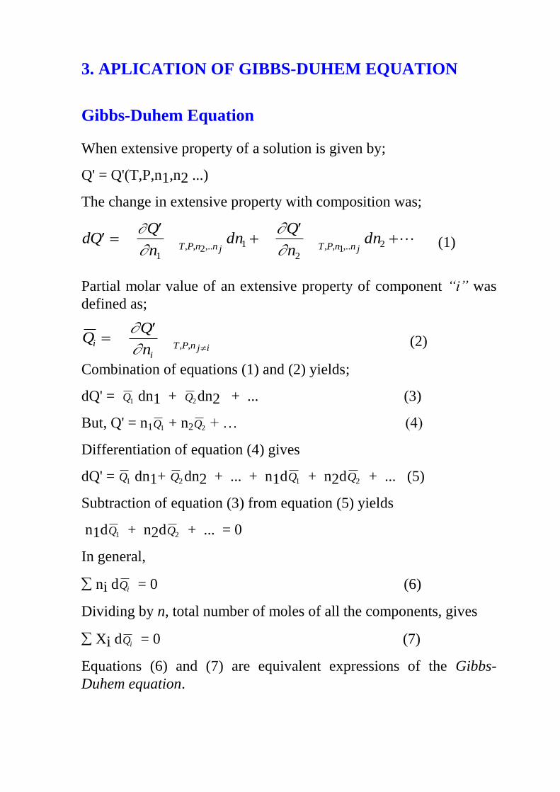
Then, previous problem for Fe-Ni alloys at 1600oC requires

integration of;

XNi 1 0.9 0.8 0.7 0.6 0.5 0.4 0.3 0.2 0.1 0

aNi 1 0.89 0.766 0.62 0.485 0.374 0.283 0.207 0.136 0.067

GNixs 0 -41.4 -161 -450 -789 -1077 -1283 -1376 -1430 -1485 RT ln

Ni cal/mol

XNi/XFe 9 4 2.33 1.5 1 0.67 0.43 0.25 0.11 0

log Ni 0 -.005 -.019 -.053 -.092 -.126 -.15 -.161 -.167 -.174 log Ni

G at XFexs

Fe( ) -G

Nixs at X Fe

GNixs at X Fe

Ni

Fe

NixsX

XdG

( )

( )

1

XNi/XFe

RT ln Nio

-1530

-GNixs

This is good for values XFe=1 to XFe > 0. As XFe 0; XNi/XFe

. Therefore, G at XFexs

Fe( ) 0 is mathematically indeterminate with

excess properties.

The use of -Function:

Problems arising from X1/X2 as X20 may be resolved using

this function. For any component i, i is defined as:

iixs

i

Q

X

( )1 2

For 1-2 binary solution from previous relationships

Q at Xxs2 2( ) -

Q xs at X

Q xs at X

xsX

XdQ

1 2 1

1 21

2

1

( )

( )

From above relationship Q Xxs1 1 2

2

Then dQ d X X dXxs1 1 2

21 2 22

Replacing into the integral yields

Q at Xxs2 2( ) -

1 2 1

1 21

2

22

1

( )

( )

at X

at XX

XX d

- X

XX

XX dX

2 1

21

2

1 2 22

Q at Xxs2 2( ) -

1 2 1

1 2

1 2 1( )

( )

at X

at X

X X d

- X

X

X dX2 1

2

1 1 22

By virtue of identity d(xy) = y dx + x dy, the first integral

1 2 1

1 2

1 2 1( )

( )

at X

at X

X X d

= d X X( )1 2 1 - 1 1 2d X X( )

Then,

Q at Xxs2 2( ) - d X X( )1 2 1 + 1 1 2d X X( ) - 2 1 1 2 X dX

= - X X1 2 1 + 1 1 2X dX + 1 2 1X dX - 2 1 1 2 X dX

= - X X1 2 1 - 1 1 1 2 22( )X X X dX

= - X X1 2 1 - X

X

dX2 1

2

1 2

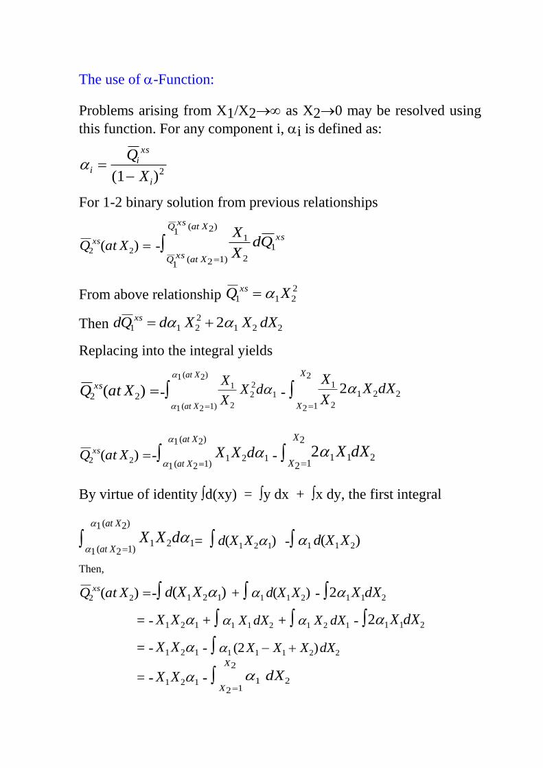
Numerical value for -X1X21 can be determined, then the value of

the integral can be determined graphically or analytically (if an

analytical expression for the composition dependence of 1 or other

properties that leads to determine 1 given). Analytical integration

with -function can be done by replacing 1 into the equation and

integrating it between the given limits. Graphical determination can

be done from the area under X2 vs. 1 graph.

1

X2

X

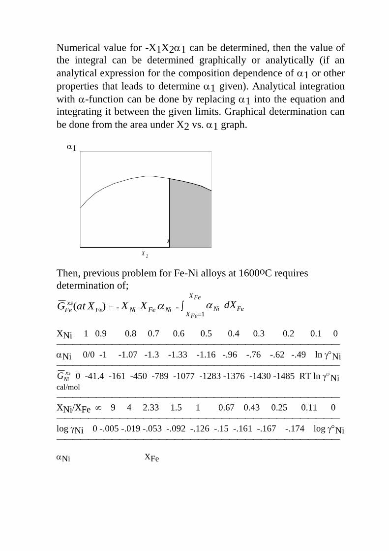
Then, previous problem for Fe-Ni alloys at 1600oC requires

determination of;

G at XFexs

Fe( ) = - X XNi Fe Ni - X Fe

X Fe

Ni FedX1

XNi 1 0.9 0.8 0.7 0.6 0.5 0.4 0.3 0.2 0.1 0

Ni 0/0 -1 -1.07 -1.3 -1.33 -1.16 -.96 -.76 -.62 -.49 ln Ni

GNixs

0 -41.4 -161 -450 -789 -1077 -1283 -1376 -1430 -1485 RT ln Ni cal/mol

XNi/XFe 9 4 2.33 1.5 1 0.67 0.43 0.25 0.11 0

log Ni 0 -.005 -.019 -.053 -.092 -.126 -.15 -.161 -.167 -.174 log Ni

Ni XFe

.5

1

1.5

For XFe = 0.7

ln Fe = -0.3 x 0.7 (-0.76) - (0.3 x 0.4 + 0.36 x 0.3 x 0.5) = 0.1596 - 0.174

ln Fe = - 0.0144; Fe = 0.985; aFe = 0.6895

Direct Calculation of the Integral Property

Consider a 2 component system, say Q1 is given. Q is asked. Indirect

method involves determination of Q2 by Gibbs-Duhem integration,

then computation of the integral property from

Q = X1 Q1 + X2 Q2

but

Q1 = Q + (1 - X1) (dQ/dX1)

multiply both sides by dX1 and divide by X22, then

Q dX

X

QdX X dQ

X

1 1

22

1 1

22

1

( )

Replacing (1 - X1) = X2 and dX1 = - dX2

Q dX

X

QdX X dQ

Xd

Q

X

1 1

22

2 2

22

2

( )

Integration of both sides

Q

Xat X

Q

X

dQ

X2

2 1

2

2( )

( )

= X

X Q dX

X1 0

11 1

22

Q

XQo

2

2 = X

X Q dX

X1 0

11 1

22

Using relative partial molar properties and setting QM at X2=1 to

zero;

Q

X

M

2

= X

X MQ dX

X1 0

11 1

22

or QM = X2 X

X MQ dX

X1 0

11 1

22

Equivalent relationship from partial excess properties and setting

Qxs at X2=1 to zero;

Qxs = X2 X

X xsQ dX

X1 0

11 1

22

Values of integrals can be obtained either analytically (if analytical

dependence of Q1 or Q M1 or Q xs

1 to composition is given) or

graphically. Analytical integration involves the following steps:

i. The replacement of the property (Q1 or Q M1 or Q

xs1 ) into the

integral.

ii. Organization of the function inside the integral in such a way to

leave only one variable.

iii. Integration and replacement of the limits.

Graphical integration involves the determination of the area under

the curve (Q X1 22

or Q XM1 2

2 or Q Xxs

1 22

vs. X1 between the limits.

X1 0 .1 .2 .3 .4 .5 .6 .7 .8 .9 1

Gxs

1 RT ln 1 .. .. .. .. .. .. .. .. .. ..

G Xxs1 2

2RT ln 1 .. .. .. .. .. .. .. .. .. ..

G Xxs1 2

2

X X1