Review of Chemical Equilibrium — IntroductionCopyright c© 2018 by Nob Hill Publishing, LLC

This chapter is a review of the equilibrium state of a system that can undergochemical reaction

Operating reactors are not at chemical equilibrium, so why study this?

Find limits of reactor performance

Find operations or design changes that allow these restrictions to be changedand reactor performance improved

1 / 76

Thermodynamic system

T ,P ,nj

Variables: temperature, T , pressure, P , the number of moles of each component,nj , j = 1, . . . ,ns.Specifying the temperature, pressure, and number of moles of each componentthen completely specifies the equilibrium state of the system.

2 / 76

Gibbs Energy

The Gibbs energy of the system, G , is the convenient energy function ofthese state variables

The difference in Gibbs energy between two different states

dG = −SdT + VdP +∑

j

µjdnj

S is the system entropy,V is the system volume andµj is the chemical potential of component j.

3 / 76

Condition for Reaction Equilibrium

Consider a closed system. The nj can change only by the single chemical reaction,

ν1A1 + ν2A2 -⇀↽- ν3A3 + ν4A4

∑j

νjAj = 0

Reaction extent.dnj = νjdε

Gibbs energy.dG = −SdT + VdP +

∑j

(νjµj

)dε (3.2)

For the closed system, G is only a function of T ,P and ε.

4 / 76

Partial derivatives

dG = −SdT + VdP +∑

j

(νjµj

)dε

S = −(∂G∂T

)P ,ε

(3.3)

V =(∂G∂P

)T ,ε

(3.4)

∑j

νjµj =(∂G∂ε

)T ,P

(3.5)

5 / 76

G versus the reaction extent

G

∂G∂ε=∑

j

νjµj = 0

ε

A necessary condition for the Gibbs energy to be a minimum∑j

νjµj = 0 (3.6)

6 / 76

Other forms: activity, fugacity

µj = G◦j + RT lnaj

aj is the activity of component j in the mixture referenced to some standardstate

G◦j is the Gibbs energy of component j in the same standard state.

The activity and fugacity of component j are related by

aj = fj/f ◦j

fj is the fugacity of component jf ◦j is the fugacity of component j in the standard state.

7 / 76

The Standard State

The standard state is: pure component j at 1.0 atm pressure and the systemtemperature.

G◦j and f ◦j are therefore not functions of the system pressure or composition

G◦j and f ◦j are strong functions of the system temperature

8 / 76

Gibbs energy change of reaction

µj = G◦j + RT lnaj

∑j

νjµj =∑

j

νjG◦j + RT∑

j

νj lnaj (3.8)

The term∑

j νjG◦j is known as the standard Gibbs energy change for the reaction,∆G◦.

∆G◦ + RT ln∏

j

aνjj = 0 (3.9)

9 / 76

Equilibrium constant

K = e−∆G◦/RT (3.10)

Another condition for chemical equilibrium

K =∏

j

aνjj (3.11)

K also is a function of the system temperature, but not a function of the systempressure or composition.

10 / 76

Ideal gas equilibrium

The reaction of isobutane and linear butenes to branched C8 hydrocarbons is usedto synthesize high octane fuel additives.

isobutane+ 1–butene -⇀↽- 2,2,3–trimethylpentane

I+ B -⇀↽- P

Determine the equilibrium composition for this system at a pressure of 2.5 atmand temperature of 400K. The standard Gibbs energy change for this reaction at400K is −3.72 kcal/mol [5].

11 / 76

Solution

The fugacity of a component in an ideal-gas mixture is equal to its partial pressure,

fj = Pj = yjP (3.12)

f ◦j = 1.0 atm because the partial pressure of a pure component j at 1.0 atm totalpressure is 1.0 atm. The activity of component j is then simply

aj =Pj

1 atm(3.13)

K = aP

aIaB(3.14)

12 / 76

Solution (cont.)

K = e−∆G◦/RT

K = 108

K = PP

PIPB= yP

yIyBP

in which P is 2.5 atm. Three unknowns, one equation,∑j

yj = 1

Three unknowns, two equations. What went wrong?

13 / 76

Ideal-gas equilibrium, revisited

Additional information. The gas is contained in a closed vessel that is initiallycharged with an equimolar mixture of isobutane and butene.Let nj0 represent the unknown initial number of moles

nI = nI0 − εnB = nB0 − εnP = nP0 + ε (3.16)

Summing Equations 3.16 produces

nT = nT 0 − ε

in which nT is the total number of moles in the vessel.

14 / 76

Moles to mole fractions

The total number of moles decreases with reaction extent because more moles areconsumed than produced by the reaction. Dividing both sides of Equations 3.16by nT produces equations for the mole fractions in terms of the reaction extent,

yI =nI0 − εnT 0 − ε

yB =nB0 − εnT 0 − ε

yP =nP0 + εnT 0 − ε

Dividing top and bottom of the right-hand side of the previous equations by nT 0

yields,

yI =yI0 − ε′1− ε′ yB =

yB0 − ε′1− ε′ yP =

yP0 + ε′1− ε′

in which ε′ = ε/nT 0 is a dimensionless reaction extent that is scaled by the initialtotal number of moles.

15 / 76

One equation and one unknown

K = (yP0 + ε′)(1− ε′)(yB0 − ε′)(yI0 − ε′)P

(yB0 − ε′)(yI0 − ε′)KP − (yP0 + ε′)(1− ε′) = 0

Quadratic in ε′. Using the initial composition, yP0 = 0, yB0 = yI0 = 1/2 gives

ε′2(1+ KP)− ε′(1+ KP)+ (1/4)KP = 0

The two solutions are

ε′ = 1±√

1/(1+ KP)2

(3.19)

16 / 76

Choosing the solution

The correct solution is chosen by considering the physical constraints that molefractions must be positive.The negative sign is therefore chosen, and the solution is ε′ = 0.469.The equilibrium mole fractions are then computed from Equation 3.18 giving

yI = 5.73× 10−2

yB = 5.73× 10−2

yP = 0.885

The equilibrium at 400K favors the product trimethylpentane.

17 / 76

Second derivative of G .

Please read the book for this discussion.I will skip over this in lecture.

18 / 76

Evaluation of G.

Let’s calculate directly G(T ,P , ε′) and see what it looks like.

G =∑

j

µjnj (3.34)

µj = G◦j + RT[ln yj + lnP

]G =

∑j

njG◦j + RT∑

j

nj[ln yj + lnP

](3.35)

For this single reaction case, nj = nj0 + νjε, which gives∑j

njG◦j =∑

j

nj0G◦j + ε∆G◦ (3.36)

19 / 76

Modified Gibbs energy

G̃(T ,P , ε′) =G −

∑j nj0G◦j

nT 0RT(3.37)

Substituting Equations 3.35 and 3.36 into Equation 3.37 gives

G̃ = ε′∆G◦

RT+∑

j

nj

nT 0

[ln yj + lnP

](3.38)

Expressing the mole fractions in terms of reaction extent gives

G̃ = −ε′ lnK +∑

j

(yj0 + νjε′)[ln

((yj0 + νjε′)

1+ νε′

)+ lnP

]

20 / 76

Final expression for the modified Gibbs Energy

G̃ = −ε′ lnK + (1+ νε′) lnP +∑

j

(yj0 + νjε′) ln(

yj0 + νjε′

1+ νε′)

(3.39)

T and P are known values, so G̃ is simply a shift of the G function up or downby a constant and then rescaling by the positive constant 1/(nT 0RT ).

The shape of the function G̃ is the same as G

The minimum with respect to ε′ is at the same value of ε′ for the twofunctions.

21 / 76

Minimum in G for an ideal gas

Goal: plot G̃ for the example and find the minimum with respect to ε′

I+ B -⇀↽- P

For this stoichiometry:∑

j νj = ν = −1.Equimolar starting mixture: yP0 = 0, yI0 = yB0 = 0.5

G̃(T ,P , ε′) = −ε′ lnK(T )+ (1− ε′) lnP+ε′ ln(ε′)+ 2(0.5− ε′) ln(0.5− ε′)− (1− ε′) ln(1− ε′) (1)

22 / 76

A picture is worth 1000 words

Recall that the range of physically significant ε′ values is 0 ≤ ε′ ≤ 0.5and what do we see...

−2

−1.5

−1

−0.5

0

0.5

1

0 0.1 0.2 0.3 0.4 0.5

−1.95

−1.94

−1.93

−1.92

−1.91

−1.9

−1.89

−1.88

0.45 0.46 0.47 0.48 0.49 0.5

G̃

ε′

23 / 76

A closer look

Good agreement with the calculated value 0.469The solution is a minimum, and the minimum is unique.

24 / 76

Effect of pressure

From Equation 3.39, for an ideal gas, the pressure enters directly in the Gibbsenergy with the lnP term.

Remake the plot for P = 2.0.

Remake the plot for P = 1.5.

How does the equilibrium composition change.

Does this agree with Le Chatelier’s principle?

For single liquid-phase or solid-phase systems, the effect of pressure onequilibrium is usually small, because the chemical potential of a component ina liquid-phase or solid-phase solution is usually a weak function of pressure.

25 / 76

Effect of temperature

The temperature effect on the Gibbs energy is contained in the lnK(T ) term.

This term often gives rise to a large effect of temperature on equilibrium.

We turn our attention to the evaluation of this important temperature effect inthe next section.

26 / 76

Evaluation of the Gibbs Energy Change of Reaction

We usually calculate the standard Gibbs energy change for the reaction, ∆G◦, byusing the Gibbs energy of formation of the species.The standard state for the elements are usually the pure elements in theircommon form at 25◦C and 1.0 atm.

G◦H2Of = G◦H2O − G◦H2− 1

2G◦O2

This gives the Gibbs energy change for the reaction at 25◦C

∆G◦i =∑

j

νijG◦jf (3.41)

27 / 76

Thermochemical Data — Where is it?

Finding appropriate thermochemical data remains a significant challenge forsolving realistic, industrial problems.

Vendors offer a variety of commercial thermochemical databases to addressthis need.

Many companies also maintain their own private thermochemical databasesfor compounds of special commercial interest to them.

Design Institute for Physical Property Data (DIPPR) database. A web-basedstudent version of the database provides students with access to data for2000 common compounds at no charge:http://dippr.byu.edu/students/chemsearch.asp.

28 / 76

Temperature Dependence of the Standard Gibbs Energy

The standard state temperature 25◦C is often not the system temperature.To convert to the system temperature, we need the temperature dependence of∆G◦

Recall from Equation 3.3 that the change of the Gibbs energy with temperature isthe negative of the entropy,(

∂G∂T

)P ,nj

= −S ,(∂G◦j∂T

)P ,nj

= −S◦j

Summing with the stoichiometric coefficients gives

∑j

∂(νjG◦j )∂T

=∑

j

−νjS◦j

Defining the term on the right-hand side to be the standard entropy change ofreaction, ∆S◦ gives

∂∆G◦

∂T= −∆S◦ (3.43)

Let H denote the enthalpy and recall its connection to the Gibbs energy,

G = H − TS (3.44)

29 / 76

Partial molar properties.

Recall the definition of a partial molar property is

X j =(∂X∂nj

)T ,P ,nk

in which X is any extensive mixture property (U,H,A,G ,V , S , etc.).

G◦j = H◦j − TS◦j

summing with the stoichiometric coefficient yields

∆G◦ = ∆H◦ − T∆S◦ (3.46)

∂∆G◦

∂T= ∆G◦ −∆H◦

T

30 / 76

van ’t Hoff equation

Rearranging this equation and division by RT gives

1RT∂∆G◦

∂T− ∆G◦

RT 2= −∆H◦

RT 2

Using differentiation formulas, the left-hand side can be rewritten as

∂(∆G◦RT

)∂T

= −∆H◦

RT 2

which finally can be expressed in terms of the equilibrium constant

∂ lnK∂T

= ∆H◦

RT 2(3.47)

31 / 76

One further approximation

∫ T2

T1

∂ lnK∂T

dT =∫ T2

T1

∆H◦

RT 2dT

If ∆H◦ is approximately constant

ln

(K2

K1

)= −∆H◦

R

(1T2− 1

T1

)(3.49)

32 / 76

Condition for Phase Equilibrium

Consider a multicomponent, multiphase system that is at equilibrium and denotetwo of the phases as α and β.T k and Pk are the temperature and pressure of phase knk

j is the number of moles of component j in phase k.

µkj is the chemical potential of component j in phase k

Phase equilibrium conditions.

T α = T β

Pα = Pβ

µαj = µβj , j = 1,2, . . . ,ns (3.50)

µj = µ◦j + RT ln fj (3.51)

If we express Equation 3.51 for two phases α and β and equate their chemicalpotentials we deduce

f αj = f βj , j = 1,2 . . . ,ns

One can therefore use either the equality of chemical potentials or fugacities asthe condition for equilibrium.

33 / 76

Gaseous Solutions

Let f Gj denote the fugacity of pure component j in the gas phase at the mixture’s

temperature and pressure.The simplest mixing rule is the linear mixing rule

f Gj = f G

j yj (ideal mixture)

An ideal gas obeys this mixing rule and the fugacity of pure j at the mixture’s Tand P is the system’s pressure, f G

j = P .

f Gj = Pyj (ideal gas)

34 / 76

Liquid (and Solid) Solutions

The simplest mixing rule for liquid (and solid) mixtures is that the fugacity ofcomponent j in the mixture is the fugacity of pure j at the mixture’s temperatureand pressure times the mole fraction of j in the mixture.

f Lj = f L

j xj

This approximation is usually valid when the mole fraction of a component is nearone.In a two-component mixture, the Gibbs-Duhem relations imply that if the firstcomponent obeys the ideal mixture, then the second component follows Henry’slaw

f L2 = k2x2

in which k2 is the Henry’s law constant for the second component.Is k2 = f L

2 ?

35 / 76

Fugacity pressure dependence.

For condensed phases, the fugacity is generally a weak function of pressure. Seethe notes for this derivation

fj∣∣

P2= fj

∣∣P1

exp

[V j(P2 − P1)

RT

](3.53)

The exponential term is called the Poynting correction factor.The Poynting correction may be neglected if the pressure does not vary by a largeamount.

36 / 76

Nonideal Mixtures

For gaseous mixtures, we define the fugacity coefficient, φj

f Gj = Pyjφj

The analogous correcting factor for the liquid phase is the activity coefficient, γj .

f Lj = f L

j xjγj

These coefficients may be available in several forms. Correlations may exist forsystems of interest or phase equilibrium data may be available from which thecoefficients can be calculated [2, 3, 6, 4, 1].

37 / 76

Equilibrium Composition for Heterogeneous Reactions

We illustrate the calculation of chemical equilibrium when there are multiplephases as well as a chemical reaction taking place.Consider the liquid-phase reaction

A(l)+ B(l) -⇀↽- C(l)

that occurs in the following three-phase system.Phase I: nonideal liquid mixture of A and C only. For illustration purposes, assumethe activity coefficients are given by the simple Margules equation,

lnγA = x2C [AAC + 2(ACA − AAC )xA]

lnγC = x2A [ACA + 2(AAC − ACA)xC ]

Phase II: pure liquid B.Phase III: ideal-gas mixture of A, B and C.

38 / 76

Phase and reaction equilibrium

All three phases are in intimate contact and we have the following data:

AAC = 1.4

ACA = 2.0

P◦A = 0.65 atm

P◦B = 0.50 atm

P◦C = 0.50 atm

in which P◦j is the vapor pressure of component j at the system temperature.

39 / 76

Phase and reaction equilibrium

1 Plot the partial pressures of A and C versus xA for a vapor phase that is inequilibrium with only the A–C liquid phase. Compute the Henry’s lawconstants for A and C from the Margules equation. Sketch the meaning ofHenry’s law on the plot and verify your calculation from the plot.

2 Use Henry’s law to calculate the composition of all three phases for K = 4.7.What is the equilibrium pressure?

3 Repeat for K = 0.23.

4 Assume K = 1. Use the Margules equation to calculate the composition of allthree phases.

5 Repeat 4 with an ideal mixture assumption and compare the results.

40 / 76

Part 1.

Equate the chemical potential in gas and liquid-phases. Since the gas phase isassumed an ideal-gas mixture:

f GA = PA gas phase, f L

A = f LA xAγA liquid phase

The fugacity of pure liquid A at the system T and P is not known.The fugacity of pure liquid A at the system temperature and the vapor pressure ofA at the system temperature is known; it is simply the vapor pressure, P◦A.If we neglect Poynting

f LA = P◦A, PA = P◦AxAγA (3.56)

The analogous expression is valid for PC .

41 / 76

Part 1.

0

0.2

0.4

0.6

0.8

1

0 0.2 0.4 0.6 0.8 1

PA

PT

PC

P◦C

P◦A

P(a

tm)

xA

42 / 76

Part 1.

Henry’s law for component A is

f LA = kAxA, f L

A = f LA xAγA

which is valid for xA small.kA = P◦AγA

which is also valid for small xA. Computing γA from the Margules equation forxA = 0 gives

γA(0) = eAAC

So the Henry’s law constant for component A is

kA = P◦AeAAC

43 / 76

Part 1.

The analogous expression holds for component C. Substituting in the values gives

kA = 2.6, kC = 3.7

The slope of the tangent line to the PA curve at xA = 0 is equal to kA.The negative of the slope of the tangent line to the PC curve at xA = 1 is equal tokC .

44 / 76

Part 2.

For K = 4.7, one expects a large value of the equilibrium constant to favor theformation of the product, C. We therefore assume that xA is small and Henry’s lawis valid for component A.The unknowns in the problem: xA and xC in the A–C mixture, yA, yB and yC in thegas phase, P .We require six equations for a well-posed problem: equate fugacities of eachcomponent in the gas and liquid phases,the mole fractions sum to one in the gas and A–C liquid phases.The chemical equilibrium provides the sixth equation.

45 / 76

Part 2.

K = aC

aAaB

aLA =

f LA

f ◦A= kAxA

f ◦Af ◦A is the fugacity of pure liquid A at the system temperature and 1.0 atm. Again,this value is unknown, but we do know that P◦A is the fugacity of pure liquid A atthe system temperature and the vapor pressure of A at this temperature.The difference between 0.65 and 1.0 atm is not large, so we assume f ◦A = P◦A.xC is assumed near one, so

aLC =

f LC

f ◦C= f L

C xC

f ◦CNow f L

C and f ◦C are the fugacities of pure liquid C at the system temperature andthe system pressure and 1.0 atm, respectively.If the system pressure turns out to be reasonably small, then it is a goodassumption to assume these fugacities are equal giving,

aLC = xC

Since component B is in a pure liquid phase, the same reasoning leads to

aLB =

f LB

f ◦B= f L

B

f ◦B= 1

46 / 76

Part 2.

Substituting these activities into the reaction equilibrium condition gives

K = xC

xAkA/P◦A · 1(3.58)

Solving Equation 3.58 for xA yields

xA =(

1+ kAKP◦A

)−1

xC =(

1+ P◦AkAK

)−1

Substituting in the provided data gives

xA = 0.05, xC = 0.95

The assumption of Henry’s law for component A is reasonable.

47 / 76

Part 2.

The vapor compositions now are computed from the phase equilibrium conditions.

PA = kAxA

PB = P◦BPC = P◦C xC

Substituting in the provided data gives

PA = 0.13 atm, PB = 0.50 atm, PC = 0.48 atm

The system pressure is therefore P = 1.11 atm.Finally, the vapor-phase concentrations can be computed from the ratios of partialpressures to total pressure,

yA = 0.12, yB = 0.45, yC = 0.43

48 / 76

Part 3.

For K = 0.23 one expects the reactants to be favored so Henry’s law is assumedfor component C. You are encouraged to work through the precedingdevelopment again for this situation. The answers are

xA = 0.97, xC = 0.03

yA = 0.51, yB = 0.40, yC = 0.09

P = 1.24 atm

Again the assumption of Henry’s law is justified and the system pressure is low.

49 / 76

Part 4.

For K = 1, we may not use Henry’s law for either A or C.In this case we must solve the reaction equilibrium condition using the Margulesequation for the activity coefficients,

K = xCγC

xAγA

Using xC = 1− xA, we have one equation in one unknown,

K =(1− xA) exp

[x2

A(ACA + 2(AAC − ACA)(1− xA))]

xA exp [(1− xA)2(AAC + 2(ACA − AAC )xA)](3.59)

50 / 76

Part 4.

Equation 3.59 can be solved numerically to give xA = 0.35.

Pj = P◦j xjγj , j = A,C

The solution isxA = 0.35, xC = 0.65

yA = 0.36, yB = 0.37, yC = 0.28

P = 1.37 atm

51 / 76

Part 5.

Finally, if one assumes that the A–C mixture is ideal, the equilibrium conditionbecomes

K = xC

xA

which can be solved to give xA = 1/(1+ K). For K = 1, the solution is

xA = 0.5, xC = 0.5

yA = 0.30, yB = 0.47, yC = 0.23

P = 1.08 atm

The ideal mixture assumption leads to significant error given the strongdeviations from ideality shown in Figure 3.4.

52 / 76

Multiple Reactions

We again consider a single-phase system but allow nr reactions∑j

νijAj = 0, i = 1,2, . . . ,nr

Let εi be the reaction extent for the ith reaction

nj = nj0 +∑

i

νijεi (3.60)

We can compute the change in Gibbs energy as before

dG = −SdT + VdP +∑

j

µjdnj

53 / 76

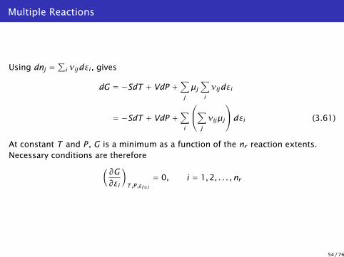
Multiple Reactions

Using dnj =∑

i νijdεi , gives

dG = −SdT + VdP +∑

j

µj

∑i

νijdεi

= −SdT + VdP +∑

i

∑j

νijµj

dεi (3.61)

At constant T and P , G is a minimum as a function of the nr reaction extents.Necessary conditions are therefore(

∂G∂εi

)T ,P ,εl≠i

= 0, i = 1,2, . . . ,nr

54 / 76

Multiple Reactions

ε2

ε1

G(εi)

∂G∂εi=∑

j

νijµj = 0

Figure 3.6: Gibbs energy versus two reaction extents at constant T and P .

Evaluating the partial derivatives in Equation 3.61 gives∑j

νijµj = 0, i = 1,2, . . . ,nr (3.62)

55 / 76

Multiple Reactions

∑j

νijµj =∑

j

νijG◦j + RT∑

j

νij lnaj

Defining the standard Gibbs energy change for reaction i, ∆G◦i =∑

j νijG◦j gives∑j

νijµj = ∆G◦i + RT∑

j

νij lnaj

Finally, defining the equilibrium constant for reaction i as

Ki = e−∆G◦i /RT (3.63)

allows one to express the reaction equilibrium condition as

Ki =∏

j

aνijj , i = 1,2, . . . ,nr (3.64)

56 / 76

Equilibrium composition for multiple reactions

In addition to the formation of 2,2,3-trimethylpentane, 2,2,4-trimethylpentanemay also form

isobutane+ 1–butene -⇀↽- 2,2,4–trimethylpentane

Recalculate the equilibrium composition for this example given that∆G◦ = −4.49 kcal/mol for this reaction at 400K.Let P1 be 2,2,3 trimethylpentane, and P2 be 2,2,4-trimethylpentane. From theGibbs energy changes, we have

K1 = 108, K2 = 284

57 / 76

Trimethyl pentane example

nI = nI0 − ε1 − ε2 nB = nB0 − ε1 − ε2 nP1 = nP10 + ε1 nP2 = nP20 + ε2

The total number of moles is then nT = nT 0 − ε1 − ε2. Forming the mole fractionsyields

yI =yI0 − ε′1 − ε′21− ε′1 − ε′2

yB =yB0 − ε′1 − ε′21− ε′1 − ε′2

yP1 =yP10 + ε′1

1− ε′1 − ε′2yP2 =

yP20 + ε′21− ε′1 − ε′2

Applying Equation 3.64 to the two reactions gives

K1 =yP1

yIyBPK2 =

yP2

yIyBP

58 / 76

Trimethyl pentane example

Substituting in the mole fractions gives two equations for the two unknownreaction extents,

PK1(yI0 − ε′1 − ε′2)(yB0 − ε′1 − ε′2)− (yP10 + ε′1)(1− ε′1 − ε′2) = 0

PK2(yI0 − ε′1 − ε′2)(yB0 − ε′1 − ε′2)− (yP20 + ε′2)(1− ε′1 − ε′2) = 0

Initial condition: yI = yB = 0.5, yP1 = yP2 = 0.

59 / 76

Numerical solution

Using the initial guess: ε1 = 0.469, ε2 = 0, gives the solution

ε1 = 0.133, ε2 = 0.351

yI = 0.031, yB = 0.031, yP1 = 0.258, yP2 = 0.680

Notice we now produce considerably less 2,2,3-trimethylpentane in favor of the2,2,4 isomer.It is clear that one cannot allow the system to reach equilibrium and still hope toobtain a high yield of the desired product.

60 / 76

Optimization Approach

The other main approach to finding the reaction equilibrium is to minimize theGibbs energy functionWe start with

G =∑

j

µjnj (3.67)

and express the chemical potential in terms of activity

µj = G◦j + RT lnaj

We again use Equation 3.60 to track the change in mole numbers due to multiplereactions,

nj = nj0 +∑

i

νijεi

61 / 76

Expression for Gibbs energy

Using the two previous equations we have

µjnj = nj0G◦j + G◦j∑

i

νijεi +nj0 +

∑i

νijεi

RT lnaj (3.68)

It is convenient to define the same modified Gibbs energy function that we used inEquation 3.37

G̃(T ,P , ε′i ) =G −

∑j nj0G◦j

nT 0RT(3.69)

in which ε′i = εi/nT 0.If we sum on j in Equation 3.68 and introduce this expression into Equations 3.67and 3.69, we obtain

G̃ =∑

i

ε′i∆G◦iRT

+∑

j

yj0 +∑

i

νijε′i

lnaj

62 / 76

Expression for G̃

G̃ = −∑

i

ε′i lnKi +∑

j

yj0 +∑

i

νijε′i

lnaj (3.70)

We minimize this modified Gibbs energy over the physically meaningful values ofthe nr extents.The main restriction on these extents is, again, that they produce nonnegativemole numbers, or, if we wish to use intensive variables, nonnegative molefractions. We can express these constraints as

−yj0 −∑

i

νijε′i ≤ 0, j = 1, . . . ,ns (3.71)

63 / 76

Optimization problem

Our final statement, therefore, for finding the equilibrium composition formultiple reactions is to solve the optimization problem

minε′i

G̃ (3.72)

subject to Equation 3.71.

64 / 76

Multiple reactions with optimization

Revisit the two-reaction trimethylpentane example, and find the equilibriumcomposition by minimizing the Gibbs energy.

aj =P

1 atmyj (ideal-gas mixture)

Substituting this relation into Equation 3.70 and rearranging gives

G̃ = −∑

i

ε′i lnKi +1+

∑i

νiε′i

lnP

+∑

j

yj0 +∑

i

νijε′i

ln

[yj0 +

∑i νijε′i

1+∑

i νiε′i

](2)

65 / 76

Constraints

The constraints on the extents are found from Equation 3.71. For this problemthey are

−yI0 + ε′1 + ε′2 ≤ 0 − yB0 + ε′1 + ε′2 ≤ 0 − yP10 − ε′1 ≤ 0 − yP20 − ε′2 ≤ 0

Substituting in the initial conditions gives the constraints

ε′1 + ε′2 ≤ 0.5, 0 ≤ ε′1, 0 ≤ ε′2

66 / 76

Solution

0

0.1

0.2

0.3

0.4

0.5

0 0.1 0.2 0.3 0.4 0.5

ε′2

ε′1

−2.559-2.55-2.53

-2.5-2-10

67 / 76

Solution

We see that the minimum is unique.The numerical solution of the optimization problem is

ε′1 = 0.133, ε′2 = 0.351, G̃ = −2.569

The solution is in good agreement with the extents computed using the algebraicapproach, and the Gibbs energy contours depicted in Figure 3.6.

68 / 76

Summary

The Gibbs energy is the convenient function for solving reaction equilibriumproblems when the temperature and pressure are specified.The fundamental equilibrium condition is that the Gibbs energy is minimized.This fundamental condition leads to several conditions for equilibrium such asFor a single reaction ∑

j

νjµj = 0

K =∏

j

aνjj

69 / 76

Summary

For multiple reactions, ∑j

νijµj = 0, i = 1, . . . ,nr

Ki =∏

j

aνijj , i = 1, . . . ,nr

in which the equilibrium constant is defined to be

Ki = e−∆G◦i /RT

70 / 76

Summary

You should feel free to use whichever formulation is most convenient for theproblem.The equilibrium “constant” is not so constant, because it depends on temperaturevia

∂ lnK∂T

= ∆H◦

RT 2

or, if the enthalpy change does not vary with temperature,

ln

(K2

K1

)= −∆H◦

R

(1T2− 1

T1

)

71 / 76

Summary

The conditions for phase equilibrium were presented: equalities oftemperature, pressure and chemical potential of each species in all phases.

The evaluation of chemical potentials of mixtures was discussed, and thefollowing methods and approximations were presented: ideal mixture,Henry’s law, and simple correlations for activity coefficients.

When more than one reaction is considered, which is the usual situation facedin applications, we require numerical methods to find the equilibriumcomposition.

Two approaches to this problem were presented. We either solve a set ofnonlinear algebraic equations or solve a nonlinear optimization problemsubject to constraints. If optimization software is available, the optimizationapproach is more powerful and provides more insight.

72 / 76

Notation I

aj activity of species jajl formula number for element l in species jAj jth species in the reaction network

CPj partial molar heat capacity of species jEl lth element constituting the species in the reaction networkfj fugacity of species jG Gibbs energyG j partial molar Gibbs energy of species j∆G◦i standard Gibbs energy change for reaction iH enthalpyH j partial molar enthalpy of species j∆H◦i standard enthalpy change for reaction ii reaction index, i = 1,2, . . . ,nr

j species index, j = 1,2, . . . ,ns

k phase index, k = 1,2, . . . ,np

K equilibrium constantKi equilibrium constant for reaction il element index, l = 1,2, . . . ,ne

nj moles of species j

73 / 76

Notation II

nr total number of reactions in reaction networkns total number of species in reaction networkP pressurePj partial pressure of species jR gas constantS entropyS j partial molar entropy of species jT temperatureV volumeV j partial molar volume of species jxj mole fraction of liquid-phase species jyj mole fraction of gas-phase species jz compressibility factor of the mixtureγj activity coefficient of species j in a mixtureε reaction extentεi reaction extent for reaction iµj chemical potential of species jνij stoichiometric number for the jth species in the ith reactionνj stoichiometric number for the jth species in a single reactionν

∑j νj

74 / 76

Notation III

νi∑

j νij

φj fugacity coefficient of species j in a mixture

75 / 76

References I

J. R. Elliott and C. T. Lira.

Introductory Chemical Engineering Thermodynamics.Prentice Hall, Upper Saddle River, New Jersey, 1999.

B. E. Poling, J. M. Prausnitz, and J. P. O’Connell.

Properties of Gases and Liquids.McGraw-Hill, New York, 2001.

J. M. Prausnitz, R. N. Lichtenthaler, and E. G. de Azevedo.

Molecular Thermodynamics of Fluid-Phase Equilibria.Prentice Hall, Upper Saddle River, New Jersey, third edition, 1999.

S. I. Sandler, editor.

Models for Thermodynamic and Phase Equilibria Calculations.Marcel Dekker, New York, 1994.

D. R. Stull, E. F. Westrum Jr., and G. C. Sinke.

The Chemical Thermodynamics of Organic Compounds.John Wiley & Sons, New York, 1969.

J. W. Tester and M. Modell.

Thermodynamics and its Applications.Prentice Hall, Upper Saddle River, New Jersey, third edition, 1997.

76 / 76