Embed Size (px)
Citation preview
REVISED ANALYSIS OF 1D ROCK SIMULATIONS FOR THE NGA-E PROJECT
Report to the PEER-Lifelines Program, Project 1C02d
Nancy Collins, Robert Graves, and Paul SomervilleURS Corporation, Pasadena Office
April 13, 2006
INTRODUCTION
This report compares the results of NGA-E 1D rock simulations of strong ground motion using three different procedures. The simulation procedures are those of PEA (Silva et al., 2002), UNR (Zeng and Anderson, 1994; Zeng, 2002), and URS (Graves and Pitarka, 2004). The three simulation procedures analyzed in this report use significantly different approaches to the representation of the earthquake source, seismic wave propagation, and site response.
The simulations described in this report were generated following the Draft Plan for 1-D Rock Motion Simulation dated July 11, 2003 (Abrahamson and Chiou, 2003). The objective of the simulations was to address the scaling issues summarized in Table 1. The simulations were performed by Walt Silva at Pacific Engineering and Analysis (PEA), Yuehua Zeng at the University of Nevada at Reno (UNR), and Robert Graves, Arben Pitarka and Nancy Collins (URS Corporation Pasadena). This report revises the results that were presented in the report entiled “Analysis of 1D Rock Simulations for the NGA-E Project,” dated October 22, 2004. The purpose of the revision is to correct errors that were found in the URS ground motion simulations. These errors are described in Appendix 1 of this report. Correction of these errors does not substantially change the conclusions of the report.
The objective of this report is to summarize and analyze the results of the 1D simulations done by these three groups (PEA, UNR, URS). The purpose of the analyses is to aid in the identification of those aspects of the simulations that may provide a reliable basis for addressing the scaling issues that are needed to guide the development of empirical models. The issues, listed in the order in which they are numbered in Table 1, are:
1. Magnitude scaling
2. and 3. Distance scaling (not addressed directly in this report)
4. Period scaling
5. Directivity scaling
6. Static stress drop scaling
7. Buried / shallow rupture scaling
8. Hanging wall / foot wall scaling
A concise summary of the results of this work is provided by Somerville et al. (2006), which is attached as Appendix 2.
Validation of Simulation Procedures
The NGA Program developed guidelines for validating the simulation procedures entitled “Validation Guidelines for Numerical Simulation of Ground Motion on Rock Conditions,” dated July 10, 2003 (Abrahamson and Chiou, 2003). The six events included in the validation program are: 1971 Imperial Valley, 1989 Loma Prieta, 1992 Landers, 1994 Northridge, 1995 Kobe, and 1999 Kocaeli. The validation of the three simulation procedures used in the 1-D simulations is described in Collins et al. (2006).
Table 1. Combinations of events needed to address specific scaling issues.
1. Mag Scaling 2. DistScaling0-10 km
3. Dist Scaling70-200
km
4. PeriodScaling
5.DirectivityScaling
6. Static
Scaling
7. Buriedvs
Shallow
8.HW / FW
EventName
Mag Stress-Drop
Dip TopOf
Rup(km)
ConstStress-Drop
Hanks and
Bakun RV SS RV SS RV SS RV SS RV SS RV Dip Mag
SA 6.5 Med 90 0 X X X X X X XSB 6.5 Low 90 0 X XSC 6.5 High 90 0 XSD 7.0 Med 90 0 X X X X XSE 7.5 Med 90 0 X X X X X XSF 7.5 Low 90 0 XSG 7.5 High* 90 0 X XSH 7.8 Med 90 0 X X X X X**SI 7.8 High* 90 0 X X**SJ 8.2 High* 90 0 XRA 6.5 Med 30 5 X XRB 6.5 Med 45 0 X X X X X XRC 6.5 Med 45 5 X XRD 6.5 Med 45 10 XRE 6.5 Med 60 5 XRF 7.0 Med 30 0 X X XRG 7.0 Med 45 0 X X X X X XRH 7.0 Med 45 5 XRI 7.0 Med 60 0 XRJ 7.5 Med 30 0 X XRK 7.5 Med 45 0 X X X X XRL 7.8 Med 30 0 X X
* These cases are the median from the Hanks and Bakun model.** These events are optional for this issue. The magnitude 7.8 cases correspond to the median areas for the Somerville et al (2003) and the Hanks and Bakun (2001) .
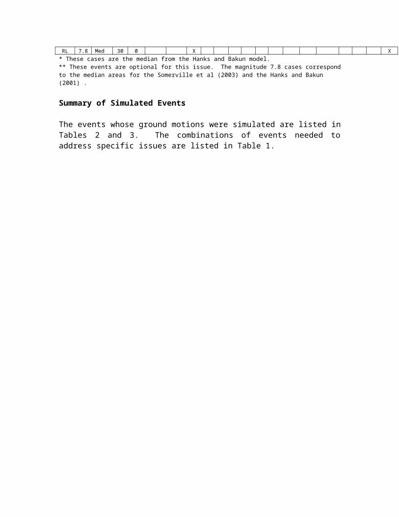
Summary of Simulated Events
The events whose ground motions were simulated are listed in Tables 2 and 3. The combinations of events needed to address specific issues are listed in Table 1.
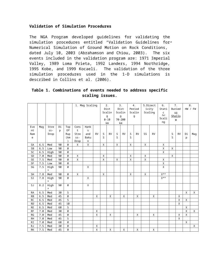
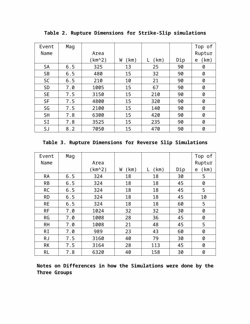
Table 2. Rupture Dimensions for Strike-Slip simulations
EventName
Mag
Area (km^2) W (km) L (km) Dip
Top of Rupture
(km)SA 6.5 325 13 25 90 0SB 6.5 480 15 32 90 0SC 6.5 210 10 21 90 0SD 7.0 1005 15 67 90 0SE 7.5 3150 15 210 90 0SF 7.5 4800 15 320 90 0SG 7.5 2100 15 140 90 0SH 7.8 6300 15 420 90 0SI 7.8 3525 15 235 90 0SJ 8.2 7050 15 470 90 0
Table 3. Rupture Dimensions for Reverse Slip Simulations
EventName
Mag
Area (km^2) W (km) L (km) Dip
Top of Rupture
(km)RA 6.5 324 18 18 30 5RB 6.5 324 18 18 45 0RC 6.5 324 18 18 45 5RD 6.5 324 18 18 45 10RE 6.5 324 18 18 60 5RF 7.0 1024 32 32 30 0RG 7.0 1008 28 36 45 0RH 7.0 1008 21 48 45 5RI 7.0 989 23 43 60 0RJ 7.5 3160 40 79 30 0RK 7.5 3164 28 113 45 0RL 7.8 6320 40 158 30 0
Notes on Differences in how the Simulations were done by the Three Groups
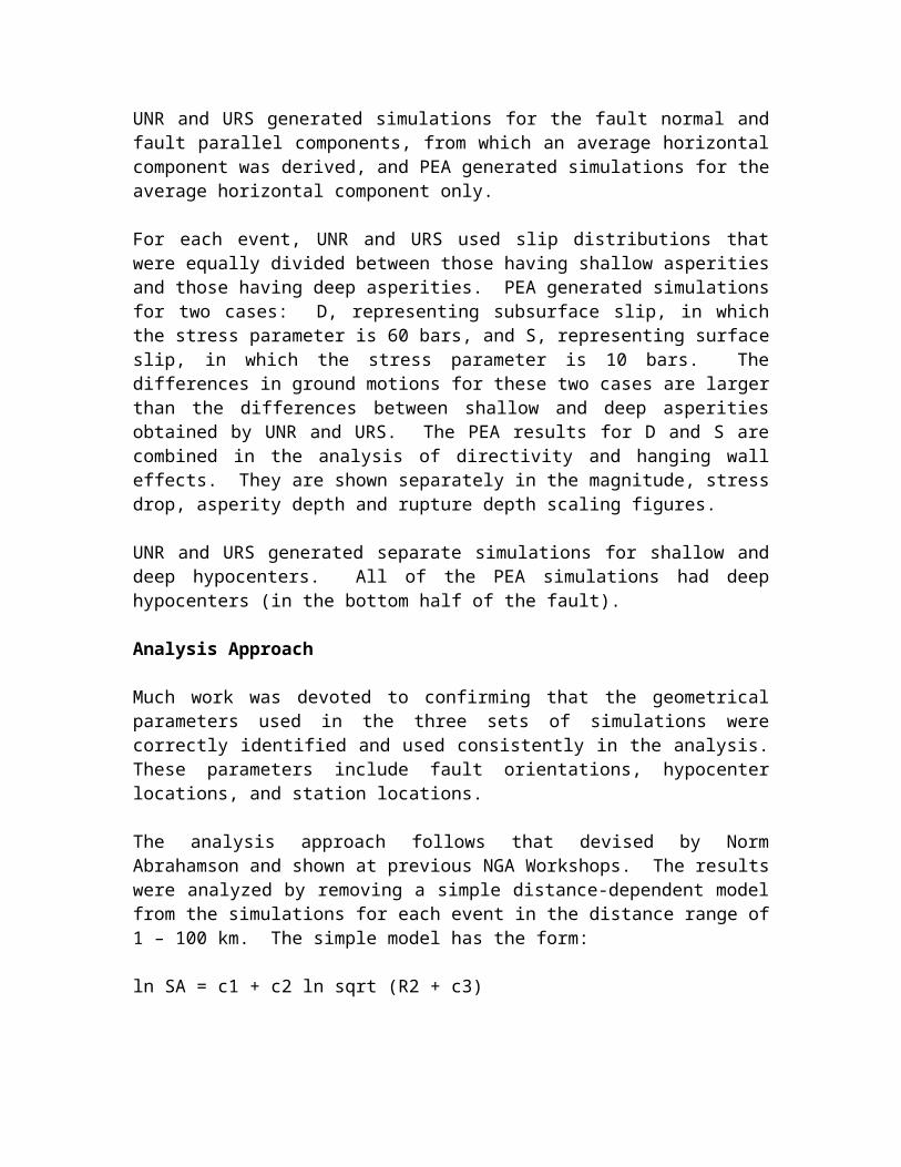
UNR and URS generated simulations for the fault normal and fault parallel components, from which an average horizontal component was derived, and PEA generated simulations for the average horizontal component only.
For each event, UNR and URS used slip distributions that were equally divided between those having shallow asperities and those having deep asperities. PEA generated simulations for two cases: D, representing subsurface slip, in which the stress parameter is 60 bars, and S, representing surface slip, in which the stress parameter is 10 bars. The differences in ground motions for these two cases are larger than the differences between shallow and deep asperities obtained by UNR and URS. The PEA results for D and S are
combined in the analysis of directivity and hanging wall effects. They are shown separately in the magnitude, stress drop, asperity depth and rupture depth scaling figures.
UNR and URS generated separate simulations for shallow and deep hypocenters. All of the PEA simulations had deep hypocenters (in the bottom half of the fault).
Analysis Approach
Much work was devoted to confirming that the geometrical parameters used in the three sets of simulations were correctly identified and used consistently in the analysis. These parameters include fault orientations, hypocenter locations, and station locations.
The analysis approach follows that devised by Norm Abrahamson and shown at previous NGA Workshops. The results were analyzed by removing a simple distance-dependent model from the simulations for each event in the distance range of 1 – 100 km. The simple model has the form:
ln SA = c1 + c2 ln sqrt (R2 + c3)
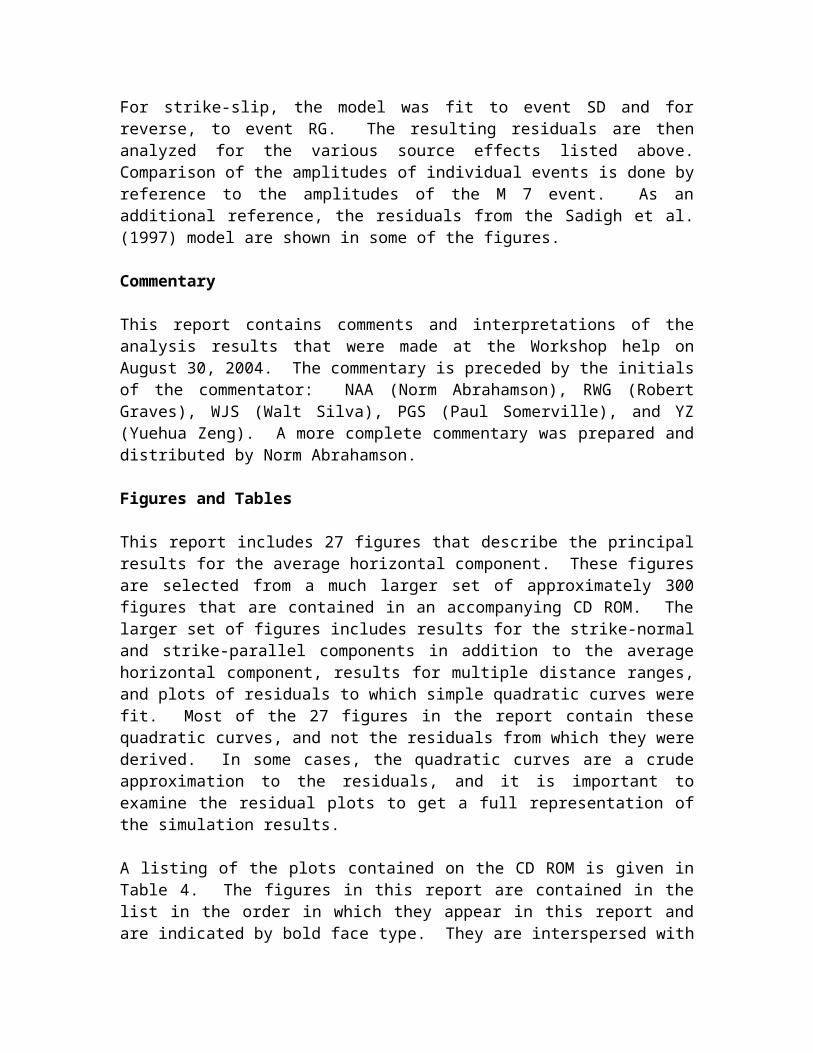
For strike-slip, the model was fit to event SD and for reverse, to event RG. The resulting residuals are then analyzed for the various source effects listed above. Comparison of the amplitudes of individual events is done by reference to the amplitudes of the M 7 event. As an additional reference, the residuals from the Sadigh et al. (1997) model are shown in some of the figures.
Commentary
This report contains comments and interpretations of the analysis results that were made at the Workshop help on August 30, 2004. The commentary is preceded by the initials of the commentator: NAA (Norm Abrahamson), RWG (Robert Graves), WJS (Walt Silva), PGS (Paul Somerville), and YZ (Yuehua Zeng). A more complete commentary was prepared and distributed by Norm Abrahamson.
Figures and Tables
This report includes 27 figures that describe the principal results for the average horizontal component. These figures are selected from a much larger set of approximately 300 figures that are contained in an accompanying CD ROM. The larger set of figures includes results for the strike-normal and strike-parallel components in addition to the average horizontal component, results for multiple distance ranges, and plots of residuals to which simple quadratic curves were fit. Most of the 27 figures in the report contain these quadratic curves, and not the residuals from which they were derived. In some cases, the quadratic curves are a crude approximation to the residuals, and it is important to examine the residual plots to get a full representation of the simulation results.
A listing of the plots contained on the CD ROM is given in Table 4. The figures in this report are contained in the list in the order in which they appear in this report and are indicated by bold face type. They are interspersed with the additional figures on the CD ROM. Titles of figures indicate their contents.
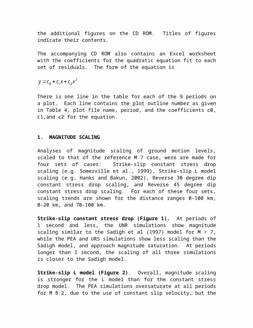
The accompanying CD ROM also contains an Excel worksheet with the coefficients for the quadratic equation fit to each set of residuals. The form of the equation is
There is one line in the table for each of the 9 periods on a plot. Each line contains the plot outline number as given in Table 4, plot file name, period, and the coefficients c0, c1,and c2 for the equation.
1. MAGNITUDE SCALING
Analyses of magnitude scaling of ground motion levels, scaled to that of the reference M 7 case, were are made for four sets of cases: Strike-slip constant stress drop scaling (e.g. Somerville et al., 1999), Strike-slip L model scaling (e.g. Hanks and Bakun, 2002), Reverse 30 degree dip constant stress drop scaling, and Reverse 45 degree dip constant stress drop scaling. For each of these four sets, scaling trends are shown for the distance ranges 0-100 km, 0-20 km, and 70-100 km.
Strike-slip constant stress drop (Figure 1). At periods of 1 second and less, the UNR simulations show magnitude scaling similar to the Sadigh et al (1997) model for M > 7, while the PEA and URS simulations show less scaling than the Sadigh model, and approach magnitude saturation. At periods longer than 1 second, the scaling of all three simulations is closer to the Sadigh model.
Strike-slip L model (Figure 2). Overall, magnitude scaling is stronger for the L model than for the constant stress drop model. The PEA simulations oversaturate at all periods for M 8.2, due to the use of constant slip velocity, but the other two simulations do not. The URS simulations have scaling similar to Sadigh for periods up to 1 second, and stronger scaling for periods longer than 1 second. The UNR simulations have scaling that is stronger than Sadigh at all periods, and have no saturation. NAA: Oversaturation is consistent with empirical data but not for long periods (T>5 sec)
Reverse 30 degree dip (Figure 3). The URS simulations have scaling similar to Sadigh, with no saturation, the PEA simulations tend to saturate at M 7.5, and the UNR simulations oversaturate at M 7.5.
Reverse 45 degree dip (Figure 4). For periods up to 2 seconds, the UNR simulations show magnitude scaling similar to the Sadigh model for M > 7, while the PEA and URS simulations show less scaling than the Sadigh model. At periods of 3 seconds and longer, the UNR simulations tend to saturate but the PEA and URS simulations do not.
NAA: Why does the UNR model show saturation for reverse slip and not for strike-slip? YZ thinks that it is related to the slip models from Beroza and Guatteri (2003), but he is not sure.
2. and 3. DISTANCE SCALING.
Distance scaling per se is not addressed in this report, but several effects are analyzed in several period ranges: 0-100 km, 0-20 km, 70-100 km.
4. PERIOD SCALING
The shape of the response spectrum is represented in two sets of figures. The first set shows the period-to-period derivative of the response spectrum that was fitted to the simulations of each event (Figure 5). A derivative of -1 corresponds to constant velocity and a derivative of –2 corresponds to constant displacement. The second set shows the integration of the derivatives to produce a response spectrum (Figure 6). The main interest is in period scaling for periods longer than 2 seconds, so the results are shown on a that period range.
For all of the events, the URS simulated spectra have an inflection at periods between 1 and 2 seconds which becomes a trough for the two largest strike-slip events (SE and SH). Similarly, for all of the events, the PEA simulated spectra have inflections at periods of 1.0 and 1.7 seconds. These features may be artifacts of the simulation procedures.
For periods longer than 2 seconds, we expect to see a positive correlation of the derivative with magnitude, with the slope less negative for higher magnitude. This trend is strong in the PEA simulations, and is also present in the URS simulations. The UNR simulations appear to have no trend, and the opposite trend at periods longer than 7 seconds.
5. DIRECTIVITY SCALING
To examine directivity effects for a given event, we fit an event-specific regression through the data for each component (fault normal and fault parallel where available, as well as average horizontal) for each event, and then examined the dependence of residuals from this regression as a function of X cos theta and Y cos phi. We then fit a quadratic curve through the residuals as a guide to their interpretation. We also plotted the Somerville et al. (1997) model, without the modifications of Abrahamson (2000), in the period range in which it is specified (0.6 to 5 seconds).
The figures for this section are of three kinds. The first kind of figure is a summary figure that shows the quadratic curve for each of the three simulations. These are provided separately for distances of 0-20 km and for 0-100 km. These are provided for the strike-slip earthquakes for along-strike directivity (X cos theta), for reverse earthquakes for up-dip directivity (Y cos phi), and also for reverse earthquakes for along
strike directivity (X cos theta). The second kind of figure shows the fits of the quadratic curves to the residuals for the individual simulations. These are also provided in two distance ranges. The residual plots show that in some cases, the quadratic curve does not fit the residuals as well as, for example, a bilinear curve would have done. The third kind of plot shows the correlation between closest distance and Y cos phi in the reverse fault simulations. This correlation explains the influence of hanging wall effects on the way in which rupture directivity is analyzed for reverse faults.
Strike-slip, along strike directivity (Figures 7 – 10). Generally, the URS simulations have directivity effects at periods of 2 seconds and longer, the PEA simulations show a small directivity effect for periods of 5 seconds and longer, and the UNR simulations do not show directivity effects except for small effects at a period of 10 seconds for the two smaller magnitudes. For the two larger magnitude events, SE and SH, the directivity tends to saturate at small values of X cos theta in the URS and PEA simulations, and then decline slowly; the quadratic fit to the residuals typically exaggerates this decline. PGS – the URS results are compatible with the Somerville et al. (1997) model for strike-slip (based on the parameter X cos theta).
Reverse, updip directivity (Figures 11-13). Generally, the URS simulations have directivity effects at periods of 2 seconds and longer, and the PEA and UNR simulations do not show directivity effects. PGS – the URS results are compatible with the Somerville et al. (1997) model for dip-slip (based on the parameter Y cos phi).
Reverse, along strike directivity (Figures 14-16). The Somerville et al. (1997) directivity model did not address along-strike directivity for reverse faults. Nevertheless, the URS simulations show along-strike directivity trends that are compatible with the trends of along strike directivity of strike-slip earthquakes in the Somerville et al. (1997) model. For the largest reverse slip event, RK, the along-strike directivity is larger than that of the Somerville et al. (1997) model for strike-slip earthquakes.
Influence of Hanging Wall Effect on the Analysis of Directivity for Reverse Faults.
To varying degrees, all three of the simulations show trends (high residuals for low values of Y cos phi) that are opposite those expected from rupture directivity for dip-slip from Somerville et al. (1997). The trends in the PEA and UNR simulations have similar amplitudes, while those in the URS simulations have lower amplitudes. Stations off the ends of the fault have been excluded, but they are included in the average model from which the residuals are derived.
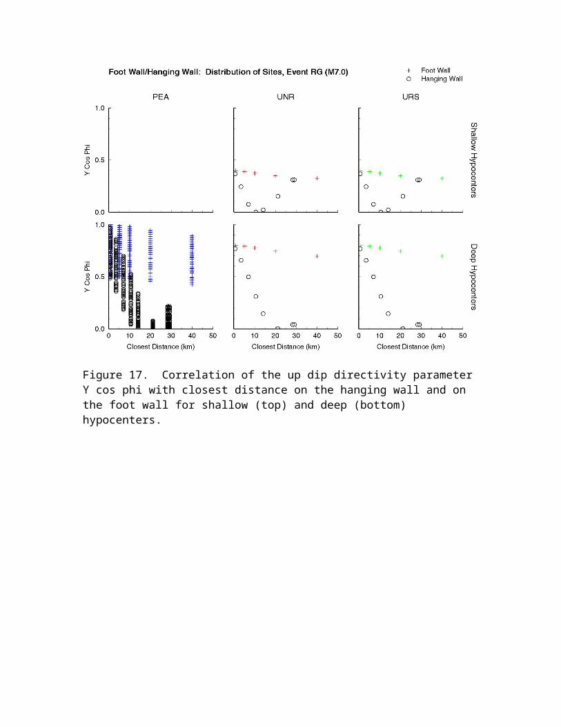
The causes of these trends are as follows. There is a strong inverse correlation between closest distance and Y cos phi, especially on the hanging wall, as pointed out in Somerville et al. (1997) and shown in the plots of Y cos phi vs. closest distance. Consequently, the rupture directivity effect is to a large extent incorporated in the average model fit through the data, and is thus absent in the residuals. What remains in the residuals is the hanging wall effect. This produces positive residuals for sites on the hanging wall, which in general have low values of Y cos phi. In contrast, most of the
foot wall sites have neutral or negative residuals but large values of Y cos phi. This causes trends that are opposite those expected for directivity from Somerville et al. (1997).
The plots of residuals vs Y cos phi for event RG, in which the foot wall and hanging wall sites are shown by different symbols, clearly show these trends (Figure 17). In the UNR and URS residual plots, there are clusters of data at Y cos phi values of about 0.4 and 0.8, corresponding to foot wall sites with shallow and deep hypocenters respectively. The intervening data points, with Y cos phi values of about 0.5 and 0.7, are hanging wall sites close to the top edge of the fault. These data points tend to have high values, especially on the fault normal component, as expected from rupture directivity.
6. STATIC STRESS DROP SCALING
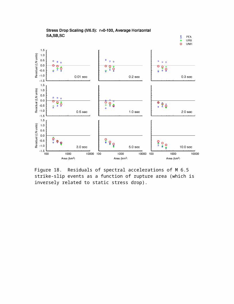
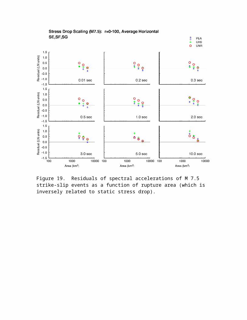
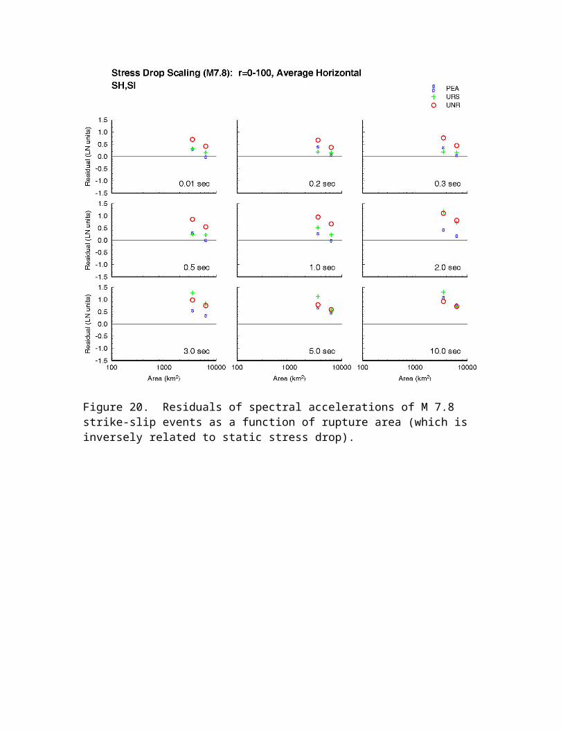
The residuals from the M 7 simulations were used to examine the dependence of spectral acceleration on stress drop. The residuals are plotted as a function of rupture area, which is inversely related to static stress drop, for each of three sets of strike-slip events: Mw 6.5, 7.5 and 7.8 (Figures 18 – 20).
For M 7.5 and 7.8, the residuals increase with increasing stress drop for all three simulations, as expected from theory, with the strongest dependency in the URS simulations, intermediate dependency in the UNR simulations, and the weakest dependency in the PEA simulations. For M 6.5, a similar pattern of scaling occurs for 5 and 10 seconds period for all three simulations, but the amount of scaling overall is weaker. For some other periods, all three simulations show departures from this pattern. The UNR simulations have little scaling between the high and median stress drop from 0.01 to 0.3 second. The PEA simulations have larger residuals for the low stress drop event than the median stress drop event from 0.01 to 1 second period. WJS – this may be the consequence of the constant slip-velocity assumption: the smaller rupture areas have larger slip which leads to a larger rise-time, reducing the ground motion. For the URS simulations, there is a complete reversal of the expected trend. RWG – the small area (high stress drop) event is dominated by shallow slip, which produces weak ground motions at short periods, while the large area (low stress drop) event is dominated by deep slip, which produces strong ground motions. NAA - Empirically, we don’t see a dependence on stress-drop.
7. BURIED vs. SHALLOW RUPTURE SCALING
Two different representations of shallow and buried rupture were examined. For reverse faults, the depth to the top of the fault was varied from 0 km (surface rupture) to 5 km and 10 km (buried rupture). For both strike-slip and reverse earthquakes, simulations were done for rupture models having both shallow and deep asperities by UNR and URS, and different stress drops (corresponding to shallow slip S and deep slip D) were used by PEA.
Depth to Top of Rupture – Reverse Faults
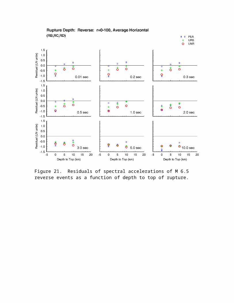
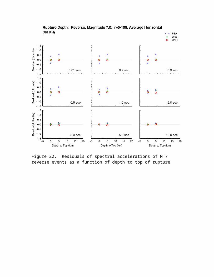
Residuals are shown as a function of depth to the top of the fault for reverse faults of magnitude 6.5 and 7 with constant stress drop but with depth to the top of the fault ranging from 0 to 5 to 10 km (Figures 21 – 22). All of the strike-slip faults extend to the surface, so there are no equivalent results for strike-slip.
At periods of 2 seconds and less, the ground motions increase with increasing depth to the top of the fault in all of the simulations, for the following reasons. For PEA, the cases at 5 and 10 km have higher stress-drop. UNR applies a scaling to the stress-drop in the top 5 km as a function of depth in the form of a taper. URS applies a longer rise-time (or lower slip velocity) in the top 5 km for all earthquakes. At periods of 5 seconds and longer, the ground motions remain constant or decrease with increasing depth for the UNR and URS simulations, but increase for the PEA simulations.
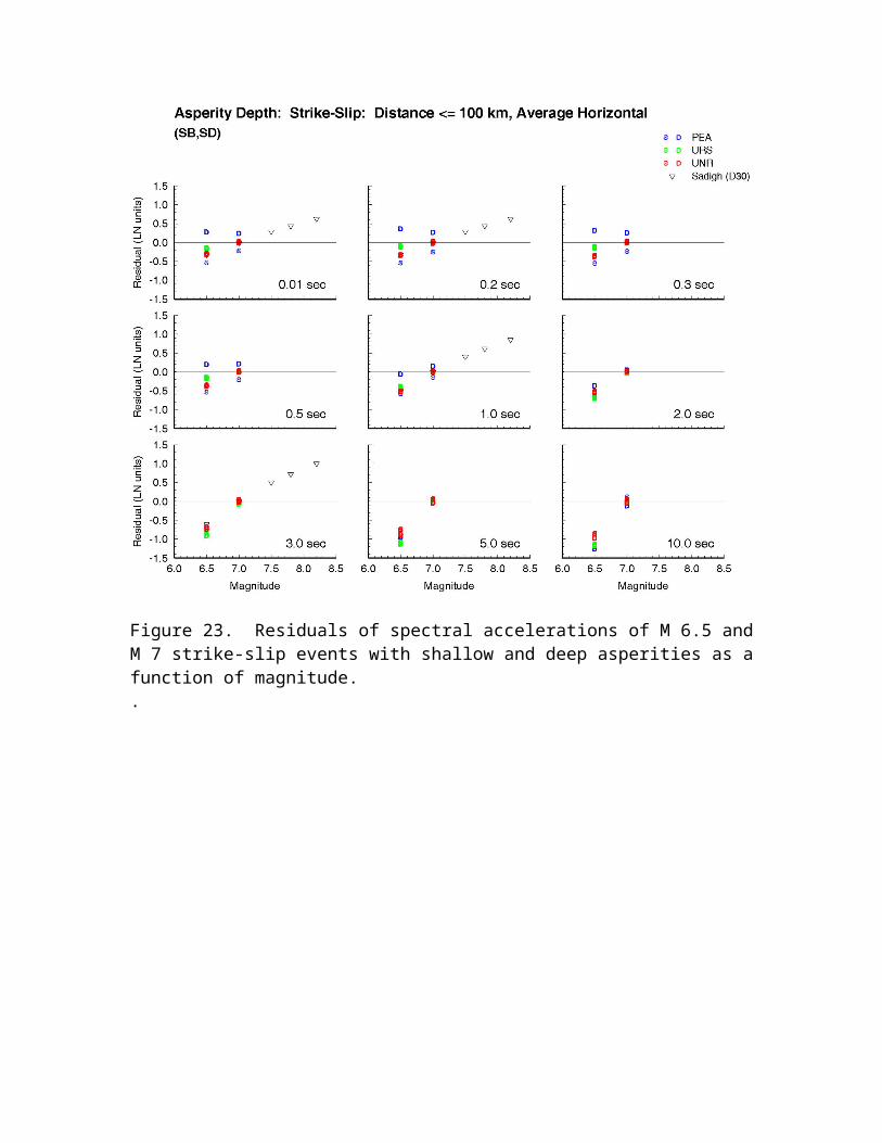
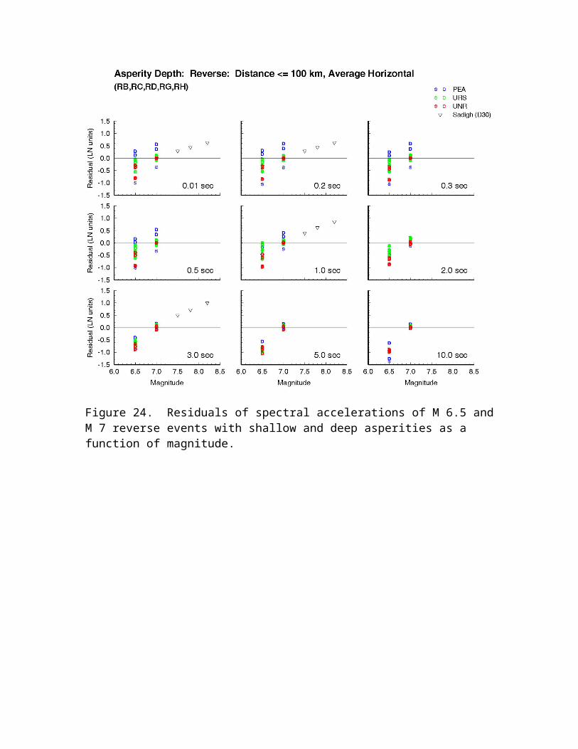
Asperity Depth – Strike-slip and Reverse Faults
Residuals are shown as a function of asperity depth for both strike-slip and dip-slip faults for two magnitudes – 6.5 and 7.0 (Figures 23 – 24).
PEA generated simulations for two cases: D – in which the stress parameter was 60 bars, and S – in which the stress parameter was 10 bars. The D case was calculated only for M 6.5 and M 7. The differences between these two cases are large at short periods and decrease at longer periods.
The UNR and URS simulations included shallow and deep asperities. The differences between ground motions for these cases are small for both strike-slip and dip-slip faults, for the following reasons. The slip models used in the UNR simulations were generated by the composite source method. UNR applied a scaling (taper) to the stress-drop in the top 5 km as a function of depth, with no change to the deep part of the fault. The slip models used in the URS simulations were generated for the NGA Project by the pseudodynamic method (Beroza and Guatteri, 2003), without consideration for the depth dependence of the shear stress on the fault. URS applied a longer rise-time (or lower slip velocity) in the top 5 km for all earthquakes, which only has an effect if there is significant slip in the top 5 km.
8. HANGING WALL / FOOT WALL SCALING
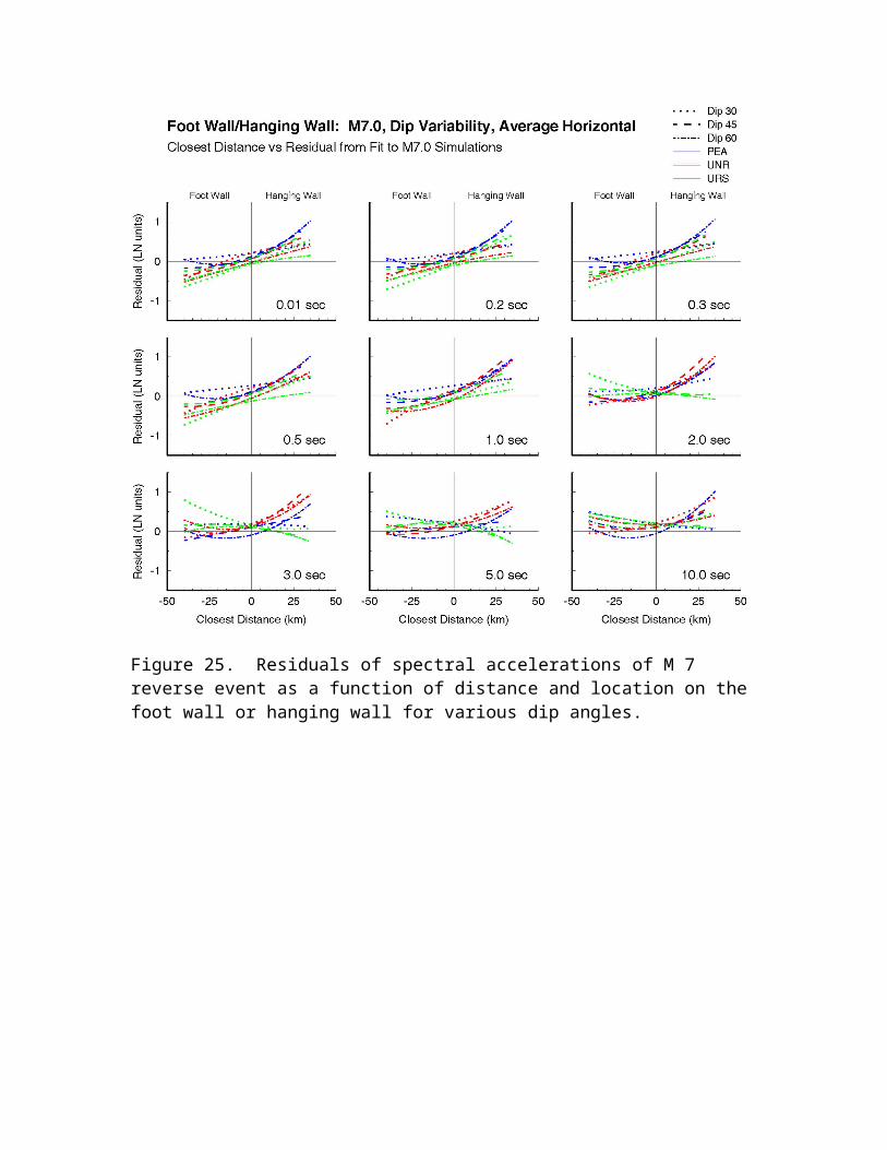
The reference for these comparisons is the ground motion model fit through the simulations for event RG (M 7). We fit a quadratic curve to the residuals to display their trends. The PEA residuals include both the D and S simulations. Stations off the ends of the fault have been excluded, but they are included in the average model from which the residuals are derived. In some cases, the quadratic form that was chosen for use does not provide a very good fit to the shape of the residuals, which would be better fitted by an S shaped curve.
Dip Angle
Magnitude 7 (Figure 25). The hanging wall trends are broadly similar between dip angles of 30, 45 and 60 degrees. The URS simulations show moderate hanging wall effects at periods from 0 to 1 second, and at periods longer than 1 second the foot wall motions equal or exceed the hanging wall motions. PGS – this period dependence conforms to the Abrahamson and Silva (1997) model. The PEA simulations show strong hanging wall effects up to 3 seconds period, beyond which the foot wall becomes stronger than the hanging wall. The UNR simulations show strong hanging wall effects at all periods. NAA: Why difference in the HW effect at long periods? May be due to difference between deep and shallow slip.
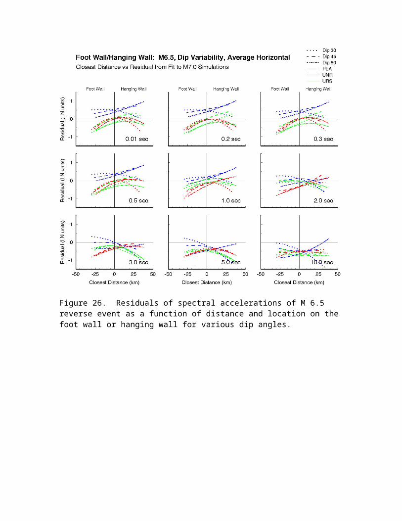
Magnitude 6.5 (Figure 26). The reference for these comparisons is magnitude 7 event RG. The hanging wall trends between dip angles of 30, 45 and 60 degrees have differences that are larger than for the magnitude 7 reference event. At periods of 0 to 1 second, the PEA simulations have much stronger hanging wall effects than the UNR and URS simulations. At periods longer than 1 second, the PEA results vary strongly with dip angle. In this period range, the UNR hanging wall levels are generally higher than those of the URS simulations.
Magnitude Scaling
The reference for these comparisons is the magnitude 7 event RG. Results are shown for four magnitudes for the three simulation teams, for a total of 12 curves for each figure (Figure 27). The results show that hanging wall effects scale strongly with magnitude. At periods of 2 seconds and longer, the UNR simulations show very different trends than the PEA and URS simulations for magnitude 6.5.
CONCLUSIONS
A concise summary of the results of this work is provided by Somerville et al. (2006a), which is attached as Appendix 2.
Strong motion simulations of ground motions for rock sites on 1D crustal models were used to guide the development of empirical models in the NGA-E Project by addressing various ground motion scaling issues. The simulation procedures were first tested against the recorded ground motions of six events, including the 1971 Imperial Valley, 1989 Loma Prieta, 1992 Landers, 1994 Northridge, 1995 Kobe, and 1999 Kocaeli earthquakes. The simulations were then used to examine the scaling of ground motion response spectra with magnitude, distance, and static stress drop (rupture area); rupture directivity effects, hanging wall / foot wall effects, and buried / shallow faulting effects. Uncertainty in the scaling of rupture area with magnitude is a key issue for the simulation of ground motions from large strikes-slip earthquakes. For constant stress drop scaling of strike-slip faults at periods of 1 second and less, the UNR simulations show magnitude scaling similar to the Sadigh et al (1997) model for M > 7, while the PEA and URS simulations show less scaling than the Sadigh model, and approach magnitude saturation. At periods
longer than 1 second, the scaling of all three simulations is closer to the Sadigh model. Overall, magnitude scaling is stronger for the L model than for the constant stress drop model.
All three simulation procedures are reasonably successful in modeling recorded ground motions (Collins et al., 2006b), giving rise to the expectation that they should produce ground motions having similar scaling relations. This expectation was only partially realized: the simulations provide some constraints on the scaling of ground motions with various source parameters, but differences in scaling relations among the three different simulation procedures can be quite large in some cases. The main cause of these differences is believed to result from discrepancies in the representation of the earthquake source used in the different procedures. This indicates the need for more rigorous testing of the simulation procedures, especially in aspects related to the characterization of the earthquake source.
REFERENCES
Abrahamson, N.A. and B. Chiou (2003). Draft Plan for 1-D Rock Motion Simulation, dated July 11, 2003.
Abrahamson, N.A. and B. Chiou (2003). Validation Guidelines for Numerical Simulation of Ground Motion on Rock Conditions, dated July 10, 2003.
Abrahamson, N.A., 2000. Effects of rupture directivity on probabilistic seismic hazard analysis. Proceedings of the 6th International Conference on Seismic Zonation, Palm Springs, Earthquake Engineering Research Institute.
Abrahamson, N.A. and W.J. Silva (1997). Empirical response spectral attenuation relations for shallow crustal earthquakes. Seism. Res. Lett. 68, 94-127.
Beroza, G.C. and M. Guatteri (2003). Physically Based Source Input for Strong Ground Motion Simulation. PEER Lifelines Final Report: Project 1C08.
Collins, N., R. Graves, and P. Somerville (2006). Comparison of Validations of Ground Motion Simulation Procedures. Report to the PEER-Lifelines Program, Project 1C02d, April 13, 2006.
Graves, R.W. and A. Pitarka (2004). Broadband time history simulation using a hybrid approach. Proceedings of the 13th World Conference on Earthquake Engineering, Vancouver, Canada, August 1-6, 2004, Paper No. 1098.
Hanks, T.C. and W.H. Bakun (2002). A bilinear source-scaling model for M-logA observations of continental earthquakes. Bull. Seism. Soc. Am, 92, 1841-1846.
Sadigh, K., C.-Y. Chang, J.A. Egan, F. Makdisi, and R.R. Youngs 1997. “Attenuation Relationships for Shallow Crustal Earthquakes Based on California Strong Motion Data”, Seismological Research Letters, Vol. 68, No. 1, pp. 180-189.
Silva, W., N. Gregor and R. Darragh (2002). Validation of 1-d numerical simulation procedures. Final Report to PEER-Lifelines Project.
Somerville, P., N. Collins, R. Graves, A. Pitarka, W. Silva, and Y. Zeng (2006). Simulation of Ground Motion Scaling Characteristics for the NGA-E Project. Proceedings of the 8th NCEE, San Francisco, April 2006.
Somerville, P.G., N.F. Smith, R.W. Graves, and N.A. Abrahamson (1997). Modification of empirical strong ground motion attenuation relations to include the amplitude and duration effects of rupture directivity, Seismological Research Letters, 68, 180-203.
Somerville, P.G., K. Irikura, R. Graves, S. Sawada, D. Wald, N. Abrahamson, Y. Iwasaki, T. Kagawa, N. Smith and A. Kowada (1999). Characterizing earthquake slip models for the prediction of strong ground motion. Seismological Research Letters, 70, 59-80.
Zeng, Y. (2002). Final Technical Report on Validation of 1-D Numerical Simulation Procedures, Final Technical Report, PEER Project 1C02, Task 1: Earthquake ground motion, Seismological Lab, University of Nevada – Reno.
Zeng Y, Anderson JG, Yu G. "A composite source model for computing synthetic strong ground motions." Geophys. Res. Lett. 1994; 21: 725-728.
Zeng, Y., J. G. Anderson and G. Yu (1994). A composite source model for computing realistic synthetic strong ground motions, J. Res. Lett., 21, 725-728.
Table 4. List of Figures on Accompanying CD ROM(Figures in boldface also appear in the report)
I. MagScl: Magnitude ScalingA. CSDM – Strike-Slip -Constant Stress Drop
1. mag-resid_csdm_0-100_avg2. mag-resid_csdm_0-100_fn3. mag-resid_csdm_0-100_fp4. mag-resid_csdm_0-20_avg5. mag-resid_csdm_0-20_fn6. mag-resid_csdm_0-20_fp7. mag-resid_csdm_70-100_avg8. mag-resid_csdm_70-100_fn9. mag-resid_csdm_70-100_fp
B. LMDL: – Strike-Slip -Hanks and Bakun - L model (4/3) Scaling1. mag-resid_lmdl_0-100_avg2. mag-resid_lmdl_0-100_fn3. mag-resid_lmdl_0-100_fp4. mag-resid_lmdl_0-20_avg5. mag-resid_lmdl_0-20_fn6. mag-resid_lmdl_0-20_fp7. mag-resid_lmdl_70-100_avg8. mag-resid_lmdl_70-100_fn9. mag-resid_lmdl_70-100_fp
C. RV30: Reverse - 30 Degree Dip1. mag-resid_rv-30_0-100_avg2. mag-resid_rv-30_0-100_fn3. mag-resid_rv-30_0-100_fp4. mag-resid_rv-30_0-20_avg5. mag-resid_rv-30_0-20_fn6. mag-resid_rv-30_0-20_fp7. mag-resid_rv-30_70-100_avg8. mag-resid_rv-30_70-100_fn9. mag-resid_rv-30_70-100_fp
D. RV45: Reverse - 45 Degree Dip1. mag-resid_rv-45_0-100_avg2. mag-resid_rv-45_0-100_fn3. mag-resid_rv-45_0-100_fp4. mag-resid_rv-45_0-20_avg5. mag-resid_rv-45_0-20_fn6. mag-resid_rv-45_0-20_fp7. mag-resid_rv-45_70-100_avg8. mag-resid_rv-45_70-100_fn9. mag-resid_rv-45_70-100_fp
II. DistScl_0-10: Distance Scaling 0-10 kmIII. DistScl_70-200: Distance Scaling 70-200 kmIV. PerScl: Period Scaling
A. Per-Deriv: Period vs Derivative of Spectral Acceleration1. per-deriv_rle20_avg2. per-deriv_rle20_fn3. per-deriv_rle20_fp4. per-deriv_allr_avg5. per-deriv_allr_fn6. per-deriv_allr_fp
B. Per-SA: Period vs Spectral Shape1. per-shape_rle20_avg2. per-shape_rle20_fn3. per-shape_rle20_fp4. per-shape_allr_avg5. per-shape_allr_fn6. per-shape_allr_fp
V. DirecScl: Directivity ScalingA. Summary_lt20km: least squares fit to residuals of all stations with closest distance < 20 km.
1. Strike-slip, along strike (x cos theta)a. xcost-resid_LSQ_SA_lt20km_avgb. xcost-resid_LSQ_SA_lt20km_fnc. xcost-resid_LSQ_SA_lt20km_fpd. xcost-resid_LSQ_SD_lt20km_avge. xcost-resid_LSQ_SD_lt20km_fnf. xcost-resid_LSQ_SD_lt20km_fpg. xcost-resid_LSQ_SE_lt20km_avgh. xcost-resid_LSQ_SE_lt20km_fni. xcost-resid_LSQ_SE_lt20km_fpj. xcost-resid_LSQ_SH_lt20km_avgk. xcost-resid_LSQ_SH_lt20km_fnl. xcost-resid_LSQ_SH_lt20km_fp
2. Reverse, updip (y cos phi)a. ycosp-resid_LSQ_RB_lt20km_avgb. ycosp-resid_LSQ_RB_lt20km_fnc. ycosp-resid_LSQ_RB_lt20km_fpd. ycosp-resid_LSQ_RG_lt20km_avge. ycosp-resid_LSQ_RG_lt20km_fnf. ycosp-resid_LSQ_RG_lt20km_fpg. ycosp-resid_LSQ_RK_lt20km_avgh. ycosp-resid_LSQ_RK_lt20km_fni. ycosp-resid_LSQ_RK_lt20km_fp
3. Reverse, along strike (x cos theta)a. xcost-resid_LSQ_RB_lt20km_avgb. xcost-resid_LSQ_RB_lt20km_fnc. xcost-resid_LSQ_RB_lt20km_fpd. xcost-resid_LSQ_RG_lt20km_avge. xcost-resid_LSQ_RG_lt20km_fnf. xcost-resid_LSQ_RG_lt20km_fpg. xcost-resid_LSQ_RK_lt20km_avgh. xcost-resid_LSQ_RK_lt20km_fni. xcost-resid_LSQ_RK_lt20km_fp
B. Summary_lt100km: least squares fit to residuals of all stations with closest distance < 100 km.1. Strike-slip, along strike (x cos theta)
a. xcost-resid_LSQ_SA_lt100km_avgb. xcost-resid_LSQ_SA_lt100km_fnc. xcost-resid_LSQ_SA_lt100km_fpd. xcost-resid_LSQ_SD_lt100km_avge. xcost-resid_LSQ_SD_lt100km_fnf. xcost-resid_LSQ_SD_lt100km_fpg. xcost-resid_LSQ_SE_lt100km_avgh. xcost-resid_LSQ_SE_lt100km_fni. xcost-resid_LSQ_SE_lt100km_fpj. xcost-resid_LSQ_SH_lt100km_avgk. xcost-resid_LSQ_SH_lt100km_fnl. xcost-resid_LSQ_SH_lt100km_fp

2. Reverse, updip (y cos phi) a. ycosp-resid_LSQ_RB_lt100km_avgb. ycosp-resid_LSQ_RB_lt100km_fnc. ycosp-resid_LSQ_RB_lt100km_fpd. ycosp-resid_LSQ_RG_lt100km_avge. ycosp-resid_LSQ_RG_lt100km_fnf. ycosp-resid_LSQ_RG_lt100km_fpg. ycosp-resid_LSQ_RK_lt100km_avgh. ycosp-resid_LSQ_RK_lt100km_fni. ycosp-resid_LSQ_RK_lt100km_fp
3. Reverse, along strike (x cos theta)a. xcost-resid_LSQ_RB_lt100km_avgb. xcost-resid_LSQ_RB_lt100km_fnc. xcost-resid_LSQ_RB_lt100km_fpd. xcost-resid_LSQ_RG_lt100km_avge. xcost-resid_LSQ_RG_lt100km_fnf. xcost-resid_LSQ_RG_lt100km_fpg. xcost-resid_LSQ_RK_lt100km_avgh. xcost-resid_LSQ_RK_lt100km_fn i. xcost-resid_LSQ_RK_lt100km_fp
C. Detail_lt20km: least squares fit to residuals of all stations with closest distance < 20 km.1. PEA
a. Strike-slip, along strike (x cos theta)1) xcost-resid_PEA_SA_lt20km_avg2) xcost-resid_PEA_SD_lt20km_avg3) xcost-resid_PEA_SE_lt20km_avg4) xcost-resid_PEA_SH_lt20km_avg
b. Reverse, updip (y cos phi)1) ycosp-resid_PEA_lt20km_RB_avg2) ycosp-resid_PEA_lt20km_RG_avg3) ycosp-resid_PEA_lt20km_RK_avg
c. Reverse, along strike (x cos theta)1) xcost-resid_PEA_RB_lt20km_avg2) xcost-resid_PEA_RG_lt20km_avg3) xcost-resid_PEA_RK_lt20km_avg
2. UNRa. Strike-slip, along strike (x cos theta)
1) xcost-resid_UNR_SA_lt20km_avg2) xcost-resid_UNR_SA_lt20km_fn3) xcost-resid_UNR_SA_lt20km_fp4) xcost-resid_UNR_SD_lt20km_avg5) xcost-resid_UNR_SD_lt20km_fn6) xcost-resid_UNR_SD_lt20km_fp7) xcost-resid_UNR_SE_lt20km_avg8) xcost-resid_UNR_SE_lt20km_fn9) xcost-resid_UNR_SE_lt20km_fp10) xcost-resid_UNR_SH_lt20km_avg11) xcost-resid_UNR_SH_lt20km_fn12) xcost-resid_UNR_SH_lt20km_fp
b. Reverse, updip (y cos phi)1) ycosp-resid_UNR_RB_lt20km_avg2) ycosp-resid_UNR_RB_lt20km_fn3) ycosp-resid_UNR_RB_lt20km_fp4) ycosp-resid_UNR_RG_lt20km_avg5) ycosp-resid_UNR_RG_lt20km_fn6) ycosp-resid_UNR_RG_lt20km_fp
7) ycosp-resid_UNR_RK_lt20km_avg8) ycosp-resid_UNR_RK_lt20km_fn9) ycosp-resid_UNR_RK_lt20km_fp
c. Reverse, along strike (x cos theta)1) xcost-resid_UNR_RB_lt20km_avg2) xcost-resid_UNR_RB_lt20km_fn3) xcost-resid_UNR_RB_lt20km_fp4) xcost-resid_UNR_RG_lt20km_avg5) xcost-resid_UNR_RG_lt20km_fn6) xcost-resid_UNR_RG_lt20km_fp7) xcost-resid_UNR_RK_lt20km_avg8) xcost-resid_UNR_RK_lt20km_fn9) xcost-resid_UNR_RK_lt20km_fp
3. URSa. Strike-slip, along strike (x cos theta)
1) xcost-resid_URS_SA_lt20km_avg2) xcost-resid_URS_SA_lt20km_fn3) xcost-resid_URS_SA_lt20km_fp4) xcost-resid_URS_SD_lt20km_avg5) xcost-resid_URS_SD_lt20km_fn6) xcost-resid_URS_SD_lt20km_fp7) xcost-resid_URS_SE_lt20km_avg8) xcost-resid_URS_SE_lt20km_fn9) xcost-resid_URS_SE_lt20km_fp10) xcost-resid_URS_SH_lt20km_avg11) xcost-resid_URS_SH_lt20km_fn12) xcost-resid_URS_SH_lt20km_fp
b. Reverse, updip (y cos phi)1) ycosp-resid_URS_RB_lt20km_avg2) ycosp-resid_URS_RB_lt20km_fn3) ycosp-resid_URS_RB_lt20km_fp4) ycosp-resid_URS_RG_lt20km_avg5) ycosp-resid_URS_RG_lt20km_fn6) ycosp-resid_URS_RG_lt20km_fp7) ycosp-resid_URS_RK_lt20km_avg8) ycosp-resid_URS_RK_lt20km_fn9) ycosp-resid_URS_RK_lt20km_fp
c. Reverse, along strike (x cos theta)1) xcost-resid_URS_RB_lt20km_avg2) xcost-resid_URS_RB_lt20km_fn3) xcost-resid_URS_RB_lt20km_fp4) xcost-resid_URS_RG_lt20km_avg5) xcost-resid_URS_RG_lt20km_fn6) xcost-resid_URS_RG_lt20km_fp7) xcost-resid_URS_RK_lt20km_avg8) xcost-resid_URS_RK_lt20km_fn9) xcost-resid_URS_RK_lt20km_fp
D. Detail_lt100km: least squares fit to residuals of all stations with closest distance < 100 km.1. PEA
a. Strike-slip, along strike (x cos theta)1) xcost-resid_PEA_SA_lt100km_avg2) xcost-resid_PEA_SD_lt100km_avg3) xcost-resid_PEA_SE_lt100km_avg4) xcost-resid_PEA_SH_lt100km_avg
b. Reverse, updip (y cos phi)1) ycosp-resid_PEA_lt100km_RB_avg
2) ycosp-resid_PEA_lt100km_RG_avg3) ycosp-resid_PEA_lt100km_RK_avg
c. Reverse, along strike (x cos theta)1) xcost-resid_PEA_RB_lt20km_avg2) xcost-resid_PEA_RG_lt20km_avg3) xcost-resid_PEA_RK_lt20km_avg
2. UNRa. Strike-slip, along strike (x cos theta)
1) xcost-resid_UNR_SA_lt20km_avg2) xcost-resid_UNR_SA_lt20km_fn3) xcost-resid_UNR_SA_lt20km_fp4) xcost-resid_UNR_SD_lt20km_avg5) xcost-resid_UNR_SD_lt20km_fn6) xcost-resid_UNR_SD_lt20km_fp7) xcost-resid_UNR_SE_lt20km_avg8) xcost-resid_UNR_SE_lt20km_fn9) xcost-resid_UNR_SE_lt20km_fp10) xcost-resid_UNR_SH_lt20km_avg11) xcost-resid_UNR_SH_lt20km_fn12) xcost-resid_UNR_SH_lt20km_fp
b Reverse, updip (y cos phi)1) ycosp-resid_UNR_RB_lt20km_avg2) ycosp-resid_UNR_RB_lt20km_fn3) ycosp-resid_UNR_RB_lt20km_fp4) ycosp-resid_UNR_RG_lt20km_avg5) ycosp-resid_UNR_RG_lt20km_fn6) ycosp-resid_UNR_RG_lt20km_fp7) ycosp-resid_UNR_RK_lt20km_avg8) ycosp-resid_UNR_RK_lt20km_fn9) ycosp-resid_UNR_RK_lt20km_fp
c. Reverse, along strike (x cos theta) 1) xcost-resid_UNR_RB_lt20km_avg2) xcost-resid_UNR_RB_lt20km_fn3) xcost-resid_UNR_RB_lt20km_fp4) xcost-resid_UNR_RG_lt20km_avg5) xcost-resid_UNR_RG_lt20km_fn6) xcost-resid_UNR_RG_lt20km_fp7) xcost-resid_UNR_RK_lt20km_avg8) xcost-resid_UNR_RK_lt20km_fn9) xcost-resid_UNR_RK_lt20km_fp
3. URSa. Strike-slip, along strike (x cos theta)
1) xcost-resid_URS_SA_lt20km_avg2) xcost-resid_URS_SA_lt20km_fn3) xcost-resid_URS_SA_lt20km_fp4) xcost-resid_URS_SD_lt20km_avg5) xcost-resid_URS_SD_lt20km_fn6) xcost-resid_URS_SD_lt20km_fp7) xcost-resid_URS_SE_lt20km_avg8) xcost-resid_URS_SE_lt20km_fn9) xcost-resid_URS_SE_lt20km_fp10) xcost-resid_URS_SH_lt20km_avg11) xcost-resid_URS_SH_lt20km_fn12) xcost-resid_URS_SH_lt20km_fp
b. Reverse, updip (y cos phi)1) ycosp-resid_URS_RB_lt20km_avg
2) ycosp-resid_URS_RB_lt20km_fn3) ycosp-resid_URS_RB_lt20km_fp4) ycosp-resid_URS_RG_lt20km_avg5) ycosp-resid_URS_RG_lt20km_fn6) ycosp-resid_URS_RG_lt20km_fp7) ycosp-resid_URS_RK_lt20km_avg8) ycosp-resid_URS_RK_lt20km_fn9) ycosp-resid_URS_RK_lt20km_fp
c. Reverse, along strike (x cos theta)1) xcost-resid_URS_RB_lt20km_avg2) xcost-resid_URS_RB_lt20km_fn3) xcost-resid_URS_RB_lt20km_fp4) xcost-resid_URS_RG_lt20km_avg5) xcost-resid_URS_RG_lt20km_fn6) xcost-resid_URS_RG_lt20km_fp7) xcost-resid_URS_RK_lt20km_avg8) xcost-resid_URS_RK_lt20km_fn9) xcost-resid_URS_RK_lt20km_fp
E. DataDistribution: Closest distance vs y cos phi1. cd-ycosp_RA2. cd-ycosp_RB3. cd-ycosp_RC4. cd-ycosp_RD5. cd-ycosp_RE6. cd-ycosp_RF7. cd-ycosp_RG8. cd-ycosp_RH9. cd-ycosp_RI10. cd-ycosp_RJ11. cd-ycosp_RK12. cd-ycosp_RL
VI. StressDrop: Static Stress Drop ScalingA. area-resid_StressDrop_M65_0-100_avgB. area-resid_StressDrop_M65_0-100_fnC. area-resid_StressDrop_M65_0-100_fpD. area-resid_StressDrop_M75_0-100_avgE. area-resid_StressDrop_M75_0-100_fnF. area-resid_StressDrop_M75_0-100_fpG. area-resid_StressDrop_M78_0-100_avgH. area-resid_StressDrop_M78_0-100_fnI. area-resid_StressDrop_M78_0-100_fp
VII. AspScl: Asperity and Rupture Depth ScalingA. Rupture Depth
1. rupdep-resid_rupdep-rv65_0-100_avg2. rupdep-resid_rupdep-rv65_0-100_fn3. rupdep-resid_rupdep-rv65_0-100_fp4. rupdep-resid_rupdep-rv70_0-100_avg5. rupdep-resid_rupdep-rv70_0-100_fn6. rupdep-resid_rupdep-rv70_0-100_fp
B. Asperity Depth1. mag-resid_aspdep-ss_0-100_avg2. mag-resid_aspdep-ss_0-100_fn3. mag-resid_aspdep-ss_0-100_fp4. mag-resid_aspdep-rv_0-100_avg5. mag-resid_aspdep-rv_0-100_fn6. mag-resid_aspdep-rv_0-100_fp
VIII. HWFW: Hanging Wall/Foot WallA. SummaryPlots
1. cd-resid_FH_M7.0.avg 2. cd-resid_FH_M7.0.fn3. cd-resid_FH_M7.0.fp4. cd-resid_FH_M6.5.avg 5. cd-resid_FH_M6.5.fn6. cd-resid_FH_M6.5.fp7. cd-resid_FH_magvar.avg8. cd-resid_FH_magvar.fp9. cd-resid_FH_magvar.fn
B. IndividualPlots1. cd-resid_FH_PEA_RA_avg2. cd-resid_FH_UNR_RA_avg3. cd-resid_FH_UNR_RA_fn4. cd-resid_FH_UNR_RA_fp5. cd-resid_FH_URS_RA_avg6. cd-resid_FH_URS_RA_fn7. cd-resid_FH_URS_RA_fp8. cd-resid_FH_PEA_RC_avg9. cd-resid_FH_UNR_RC_avg10. cd-resid_FH_UNR_RC_fn11. cd-resid_FH_UNR_RC_fp12. cd-resid_FH_URS_RC_avg13. cd-resid_FH_URS_RC_fn14. cd-resid_FH_URS_RC_fp15. cd-resid_FH_PEA_RE_avg16. cd-resid_FH_UNR_RE_avg17. cd-resid_FH_UNR_RE_fn18. cd-resid_FH_UNR_RE_fp19. cd-resid_FH_URS_RE_avg20. cd-resid_FH_URS_RE_fn21. cd-resid_FH_URS_RE_fp22. cd-resid_FH_PEA_RF_avg23. cd-resid_FH_UNR_RF_avg24. cd-resid_FH_UNR_RF_fn25. cd-resid_FH_UNR_RF_fp26. cd-resid_FH_URS_RF_avg27. cd-resid_FH_URS_RF_fn28. cd-resid_FH_URS_RF_fp29. cd-resid_FH_PEA_RG_avg30. cd-resid_FH_UNR_RG_avg31. cd-resid_FH_UNR_RG_fn32. cd-resid_FH_UNR_RG_fp33. cd-resid_FH_URS_RG_avg34. cd-resid_FH_URS_RG_fn35. cd-resid_FH_URS_RG_fp36. cd-resid_FH_PEA_RI_avg37. cd-resid_FH_UNR_RI_avg38. cd-resid_FH_UNR_RI_fn39. cd-resid_FH_UNR_RI_fp40. cd-resid_FH_URS_RI_avg41. cd-resid_FH_URS_RI_fn42. cd-resid_FH_URS_RI_fp43. cd-resid_FH_PEA_RJ_avg44. cd-resid_FH_UNR_RJ_avg

45. cd-resid_FH_UNR_RJ_fn46. cd-resid_FH_UNR_RJ_fp47. cd-resid_FH_URS_RJ_avg48. cd-resid_FH_URS_RJ_fn49. cd-resid_FH_URS_RJ_fp50. cd-resid_FH_PEA_RL_avg51. cd-resid_FH_UNR_RL_avg52. cd-resid_FH_UNR_RL_fn53. cd-resid_FH_UNR_RL_fp54. cd-resid_FH_URS_RL_avg55. cd-resid_FH_URS_RL_fn56. cd-resid_FH_URS_RL_fp
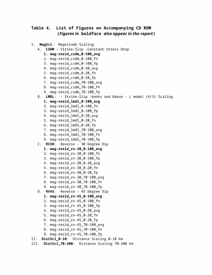
Figure Captions
Figure 1. Magnitude scaling of spectral acceleration for strike-slip earthquakes assuming constant stress drop scaling, normalized at M 7.
Figure 2. Magnitude scaling of spectral acceleration for strike-slip earthquakes assuming L model scaling (Hanks and Bakun, 2002), normalized at M 7.
Figure 3. Magnitude scaling of spectral acceleration for reverse earthquakes, dip 30 degrees, for constant stress drop scaling, normalized at M 7.
Figure 4. Magnitude scaling of spectral acceleration for reverse earthquakes, dip 45 degrees, for constant stress drop scaling, normalized at M 7.
Figure 5. Slope of the acceleration response spectrum.
Figure 6. Shape of the acceleration response spectrum, normalized at 2 seconds period.
Figure 7. Residuals of spectral accelerations of strike-slip event SA as a function of the along strike directivity parameter X cos theta.
Figure 8. Residuals of spectral accelerations of strike-slip event SD as a function of the along strike directivity parameter X cos theta.
Figure 9. Residuals of spectral accelerations of strike-slip event SE as a function of the along strike directivity parameter X cos theta.
Figure 10. Residuals of spectral accelerations of strike-slip event SH as a function of the along strike directivity parameter X cos theta.
Figure 11. Residuals of spectral accelerations of reverse event RB as a function of the up dip directivity parameter Y cos phi.
Figure 12. Residuals of spectral accelerations of reverse event RG as a function of the up dip directivity parameter Y cos phi.
Figure 13. Residuals of spectral accelerations of reverse event RK as a function of the up dip directivity parameter Y cos phi.
Figure 14. Residuals of spectral accelerations of reverse event RB as a function of the along strike directivity parameter X cos theta.
Figure 15. Residuals of spectral accelerations of reverse event RG as a function of the along strike directivity parameter X cos theta.
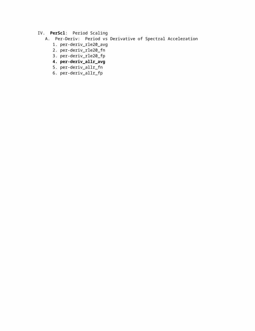
Figure 16. Residuals of spectral accelerations of reverse event RK as a function of the along strike directivity parameter X cos theta.
Figure 17. Correlation of the up dip directivity parameter Y cos phi with closest distance on the hanging wall and on the foot wall for shallow (top) and deep (bottom) hypocenters
Figure 18. Residuals of spectral accelerations of M 6.5 strike-slip events as a function of rupture area (which is inversely related to static stress drop).
Figure 19. Residuals of spectral accelerations of M 7.5 strike-slip events as a function of rupture area (which is inversely related to static stress drop).
Figure 20. Residuals of spectral accelerations of M 7.8 strike-slip events as a function of rupture area (which is inversely related to static stress drop).
Figure 21. Residuals of spectral accelerations of M 6.5 reverse events as a function of depth to top of rupture.
Figure 22. Residuals of spectral accelerations of M 7 reverse events as a function of depth to top of rupture.
Figure 23. Residuals of spectral accelerations of M 6.5 and M 7 strike-slip events with shallow and deep asperities as a function of magnitude.
Figure 24. Residuals of spectral accelerations of M 6.5 and M 7 reverse events with shallow and deep asperities as a function of magnitude.
Figure 25. Residuals of spectral accelerations of M 7 reverse event as a function of distance and location on the foot wall or hanging wall for various dip angles.
Figure 26. Residuals of spectral accelerations of M 6.5 reverse event as a function of distance and location on the foot wall or hanging wall for various dip angles.
Figure 27. Residuals of spectral accelerations of reverse events as a function of distance and location on the foot wall or hanging wall for a dip angle of 30 degrees for various magnitudes.
Figure 1. Magnitude scaling of spectral acceleration for strike-slip earthquakes assuming constant stress drop scaling, normalized at M 7.
Figure 2. Magnitude scaling of spectral acceleration for strike-slip earthquakes assuming L model scaling (Hanks and Bakun, 2002), normalized at M 7.
Figure 3. Magnitude scaling of spectral acceleration for reverse earthquakes, dip 30 degrees, for constant stress drop scaling, normalized at M 7.
Figure 4. Magnitude scaling of spectral acceleration for reverse earthquakes, dip 45 degrees, for constant stress drop scaling, normalized at M 7.
Figure 5. Slope of the acceleration response spectrum.
Figure 6. Shape of the acceleration response spectrum, normalized at 2 seconds period.
Figure 7. Residuals of spectral accelerations of strike-slip event SA as a function of the along strike directivity parameter X cos theta.
Figure 8. Residuals of spectral accelerations of strike-slip event SD as a function of the along strike directivity parameter X cos theta.
Figure 9. Residuals of spectral accelerations of strike-slip event SE as a function of the along strike directivity parameter X cos theta.
Figure 10. Residuals of spectral accelerations of strike-slip event SH as a function of the along strike directivity parameter X cos theta.
Figure 11. Residuals of spectral accelerations of reverse event RB as a function of the up dip directivity parameter Y cos phi.
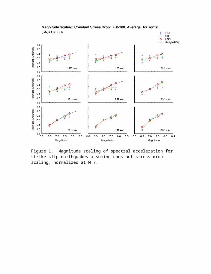
Figure 12. Residuals of spectral accelerations of reverse event RG as a function of the up dip directivity parameter Y cos phi.
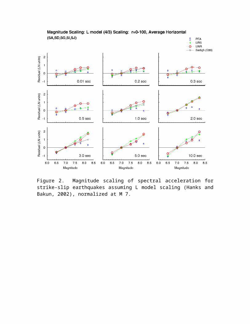
Figure 13. Residuals of spectral accelerations of reverse event RK as a function of the up dip directivity parameter Y cos phi.
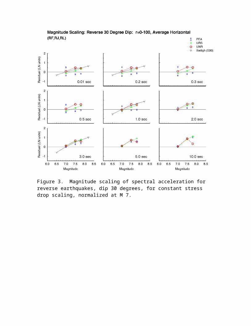
Figure 14. Residuals of spectral accelerations of reverse event RB as a function of the along strike directivity parameter X cos theta.
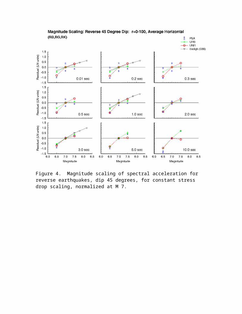
Figure 15. Residuals of spectral accelerations of reverse event RG as a function of the along strike directivity parameter X cos theta.
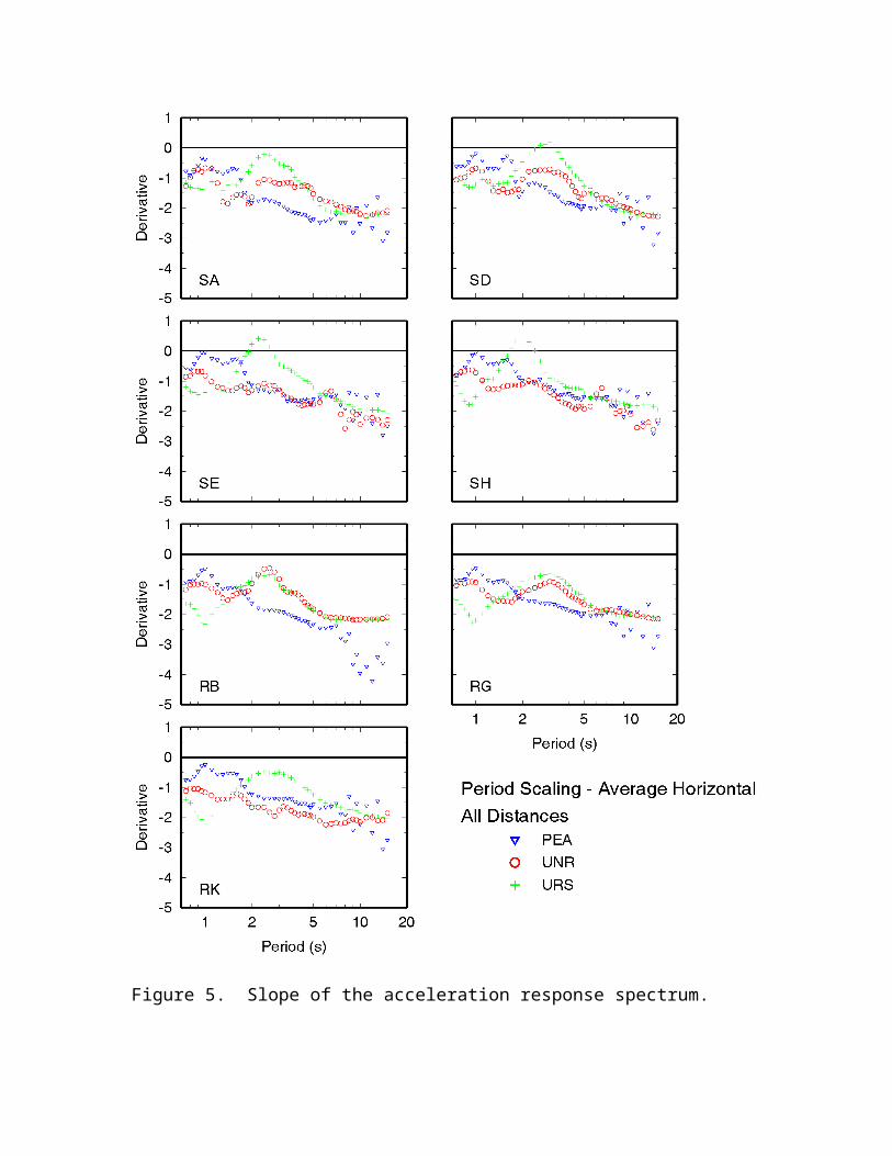
Figure 16. Residuals of spectral accelerations of reverse event RK as a function of the along strike directivity parameter X cos theta.
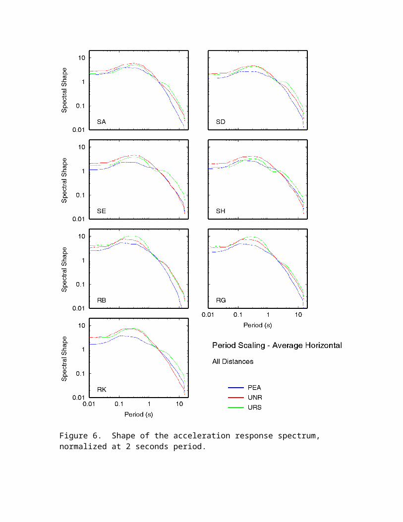
Figure 17. Correlation of the up dip directivity parameter Y cos phi with closest distance on the hanging wall and on the foot wall for shallow (top) and deep (bottom) hypocenters.
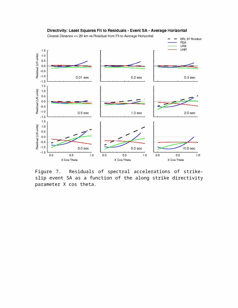
Figure 18. Residuals of spectral accelerations of M 6.5 strike-slip events as a function of rupture area (which is inversely related to static stress drop).
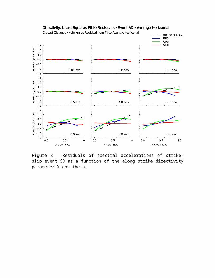
Figure 19. Residuals of spectral accelerations of M 7.5 strike-slip events as a function of rupture area (which is inversely related to static stress drop).
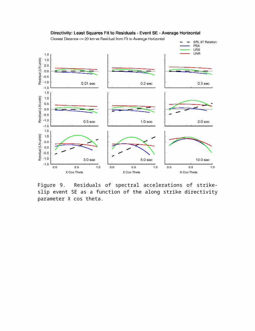
Figure 20. Residuals of spectral accelerations of M 7.8 strike-slip events as a function of rupture area (which is inversely related to static stress drop).
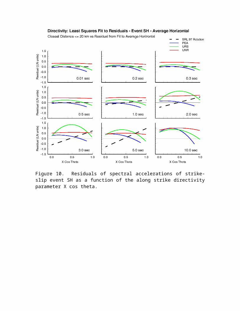
Figure 21. Residuals of spectral accelerations of M 6.5 reverse events as a function of depth to top of rupture.
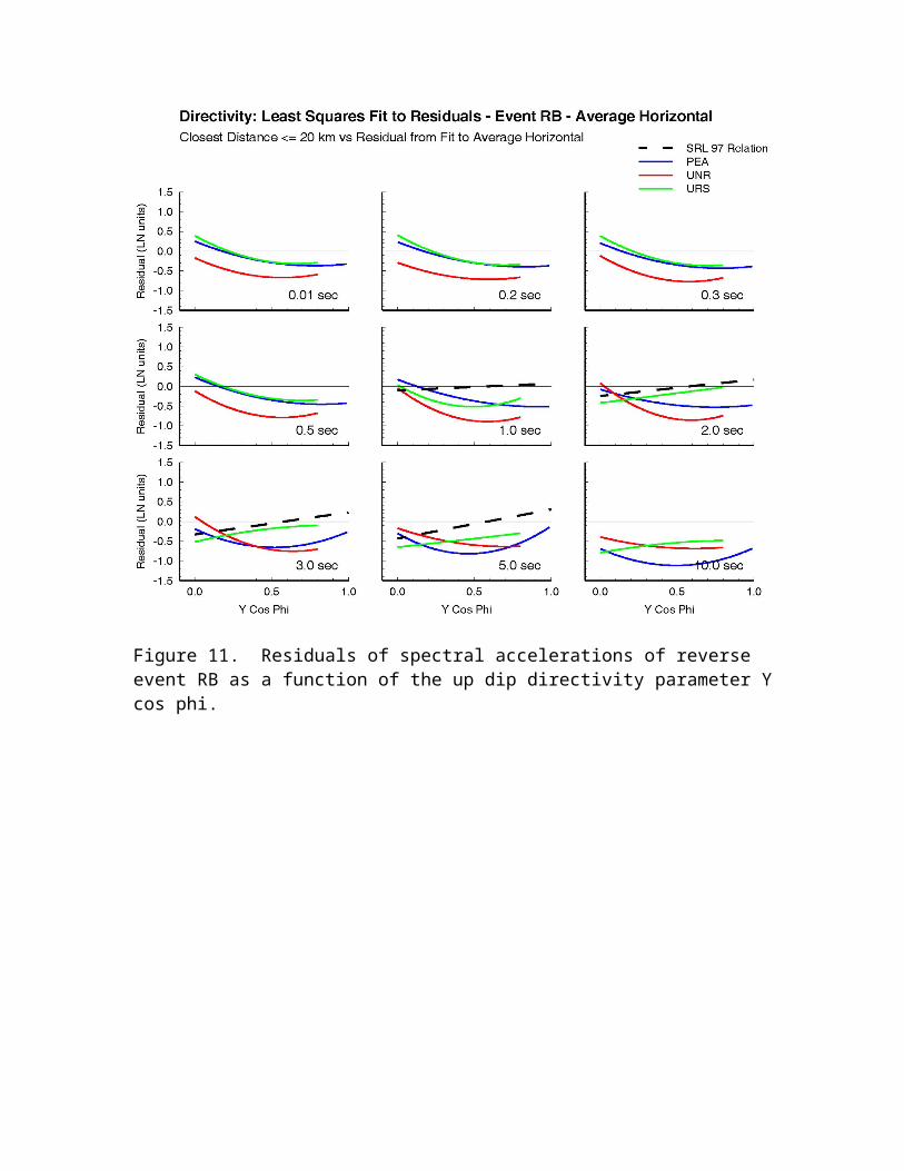
Figure 22. Residuals of spectral accelerations of M 7 reverse events as a function of depth to top of rupture
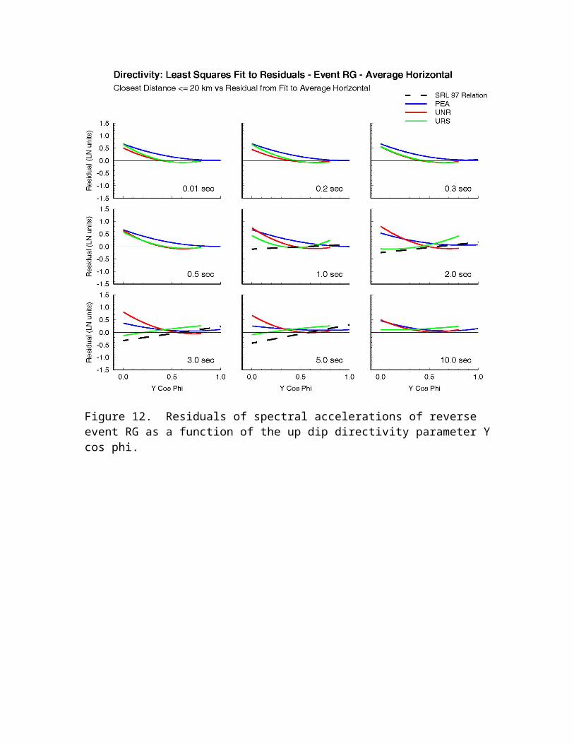
Figure 23. Residuals of spectral accelerations of M 6.5 and M 7 strike-slip events with shallow and deep asperities as a function of magnitude..
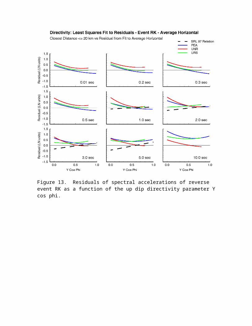
Figure 24. Residuals of spectral accelerations of M 6.5 and M 7 reverse events with shallow and deep asperities as a function of magnitude.
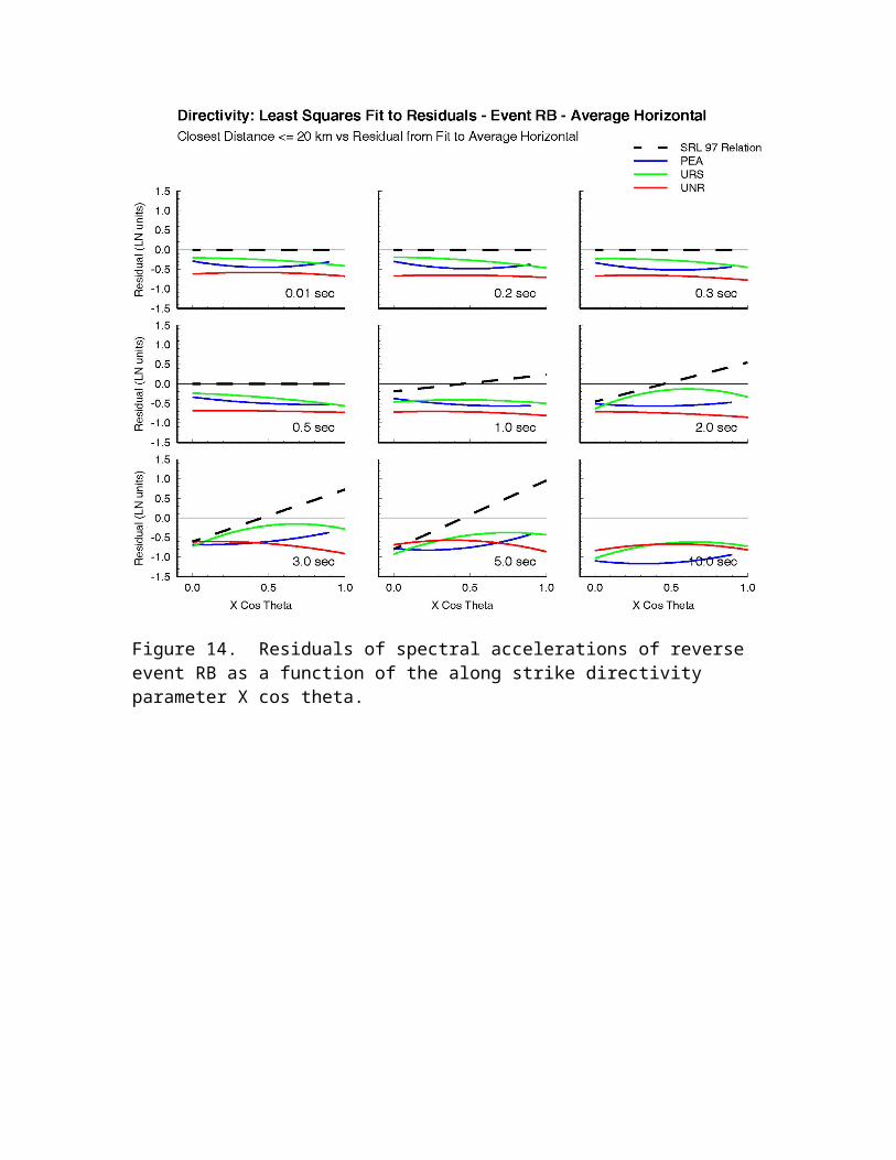
Figure 25. Residuals of spectral accelerations of M 7 reverse event as a function of distance and location on the foot wall or hanging wall for various dip angles.
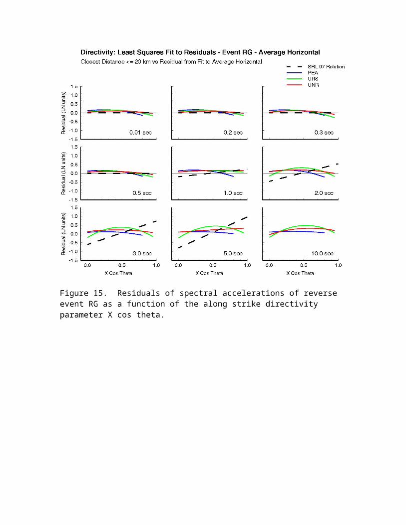
Figure 26. Residuals of spectral accelerations of M 6.5 reverse event as a function of distance and location on the foot wall or hanging wall for various dip angles.
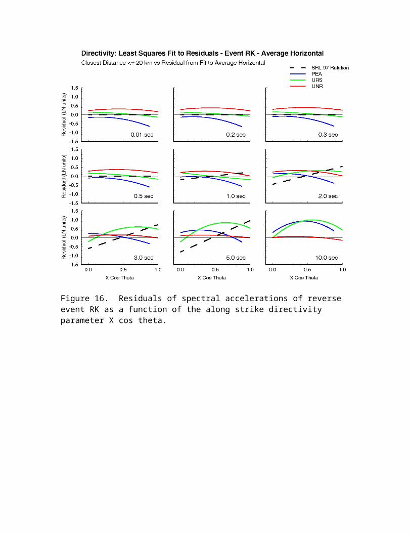
Figure 27. Residuals of spectral accelerations of reverse events as a function of distance and location on the foot wall or hanging wall for a dip angle of 30 degrees for various magnitudes.
APPENDIX 1. Updated NGA Simulation Results
Prepared by Robert Graves and Nancy CollinsDecember 2, 2005
Description of Changes
In the course of further analyzing the NGA simulation results, we discovered several errors that have subsequently been corrected. The effect of these errors on the previous set of results is minimal. That is, the general interpretation of the results is essentially unchanged, and any trends or characteristics seen in the earlier results are present in the new set of results. For completeness, we have updated all of the ground motion tables and the set of plots displaying the analyses of these results. We have compared all of the plots to the previous versions and have found no significant differences. Any changes we found appear to be minor. However, we appreciate any feedback on these new results, especially if notable differences are discovered.
Specific modifications incorporated into the December 2005 release of the tables and plots are listed below:
1) In the earlier (Oct2004) URS simulations, the time windowing for some of the strike-slip simulations omitted part of the direct arrivals. This occurred mainly at the near-fault sites for event SD, and also occurred to a lesser extent for some of the realizations for events SA, SB, SC, SE and SH. All of the affected simulations have been redone for the updated release.
2) In the earlier (Oct2004) URS simulations, the buried reverse faults were mislocated, in that the faults were dropped vertically from the top center as opposed to sliding down-dip to the specified depth (please note that the metadata for these earlier results was consistent with the fault location that was used in the simulations). We have now redone these events with the correct fault locations in order to be consistent with the other modelers and the description presented in the simulation plan. A new version of the metadata has been generated, which is consistent with the updated set of simulations. The affected events are RA, RC, RD, RE and RH.
3) Updates to metadata:
3.1) Depth to top of fault is now explicitly set to zero for surface rupturing events (URS only, previously was set at 0.1 km).
3.2) Buried reverse events have locations consistent with how the simulations were run (URS only, see 2. above).
3.3) The metadata were incorrectly calculated for event RH for PEA and UNR. These are corrected in the current table files and plots.
It should be noted that component orientation in the tables is as submitted by the modeler and follow the conventions in the table below (UNR has opposite orientation from PEA and URS).
Modeler PEA UNR URSComponentFault Normal 090 000 090Fault Parallel 000 090 000Average Horizontal avg avg avg
Effect of Prescribed Slip Distribution on Simulation Results
Several developers have inquired about the 3 second spectral peak in the URS strike-slip simulations (see Figure 1, from Brian Chiou).
The peak at 3 seconds period results from a combination of effects, listed below in order of importance:
1) smooth slip distribution2) rupture velocity3) shallow slip in 1D velocity model4) rise time
The slip models for the simulation exercise were generated and provided to NGA by Greg Beroza. URS is the only modeler group to use the slip distributions provided by Greg Beroza without modification.
These slip distributions tend to be rather smooth at the larger magnitudes, with quite elongated asperities. This results in a strong build-up of energy (both fault normal and
0.01
0.1
1
0.01 0.1 1 10
Period (sec)
Sa/
Sa[
T=0.
01]
URS; FN; 0 km <= ClstD < 20 km; 0 <= Theta.D <= 90; 0 <= X <= 1
SASBSCSD
SESFSGSH
SISJ
0.01
0.1
1
0.01 0.1 1 10
Period (sec)
Sa/
Sa[
T=0.
01]
URS; FP; 0 km <= ClstD < 20 km; 0 <= Theta.D <= 90; 0 <= X <= 1
SASBSCSD
SESFSGSH
SISJ
Figure 1: Average SA for sites within 20 km distance for URS strike-slip simulations. Fault normal on left, fault parallel on right.
fault parallel) as the rupture propagates along the fault. The presence of significant shallow slip (less than 4 km) further enhances the energy build-up due to the lower velocities in the upper 4 km of the 1D structure (i.e., energy radiated into this zone is effectively trapped in the near-surface).
We use a reference rupture velocity set at 85% of the local shear wave velocity (with further reduction in the upper 5 km). Our methodology adjusts the rupture velocity such that it increases in regions of large slip. Since the slip distributions are smooth, these adjustments are not very significant for these simulations. The result is that the rupture propagates very smoothly and coherently along the fault. Interestingly, the effect of rise time is not significant unless it is made quite long (i.e., 4-5 times larger). In fact, the waveforms at many of these near fault sites do not change dramatically, even if we use a very short rise time (e.g. 0.2 s). This suggests that the 3 second period response is controlled by the integrated effect of smooth rupture over a large distance in the prescribed 1D velocity structure.
Figure 2: Rupture model for M7.4 Izmit EQ (top). Two rupture models used for M7.5 strike-slip EQ simulations (bottom).
Furthermore, we see no evidence of this 3 second peak in any of the simulations we have done for the validation events (or in other scenario simulations we have performed with our methodology). The slip distributions used in the validation events (derived by other researchers by inversion of seismic data) show a significantly higher degree of spatial heterogeneity than the slip models provided for the simulation exercise. An example of this is shown in Figure 2, which compares the rupture model we used for the M7.4 Izmit (Kocaeli) validation with two rupture models used for the SH M7.5 simulations. The Izmit slip distribution is much rougher than the SH rupture models, and we suspect that if more heterogeneous slip models (i.e., similar to Izmit) were used for the larger magnitude simulations, then the 3 second period build-up would not be there.
Finally, the above discussion should not be taken as a blanket criticism of Beroza's slip models or his methodology for characterizing them. We believe his methodology for generating dynamically compatible rupture models is quite promising. Unfortunately, we currently don't have enough observational evidence to fully constrain what the slip distribution and rupture process should look like at the larger magnitudes. This is an area of active research, and improvements to the methodology should be forthcoming.
APPENDIX 2. From Proceedings of the 8th NCEE, San Francisco, April 2006
SIMULATION OF GROUND MOTION SCALING CHARACTERISTICS FOR THE NGA-E PROJECT
Paul Somerville1, Nancy Collins2, Robert Graves1, Arben Pitarka1, Walt Silva3, and Yehua Zeng4
ABSTRACT
Strong motion simulations of ground motions for rock sites on 1D crustal models were used to guide the development of empirical models in the NGA-E Project by addressing various ground motion scaling issues. The simulation procedures were first tested against the recorded ground motions of six events, including the 1971 Imperial Valley, 1989 Loma Prieta, 1992 Landers, 1994 Northridge, 1995 Kobe, and 1999 Kocaeli earthquakes. The simulations were then used to examine the scaling of ground motion response spectra with magnitude, distance, and static stress drop (rupture area); rupture directivity effects, hanging wall / foot wall effects, and buried / shallow faulting effects. Uncertainty in the scaling of rupture area with magnitude is a key issue for the simulation of ground motions from large strikes-slip earthquakes. For constant stress drop scaling of strike-slip faults at periods of 1 second and less, the UNR simulations show magnitude scaling similar to the Sadigh et al (1997) model for M > 7, while the PEA and URS simulations show less scaling than the Sadigh model, and approach magnitude saturation. At periods longer than 1 second, the scaling of all three simulations is closer to the Sadigh model. Overall, magnitude scaling is stronger for the L model than for the constant stress drop model. Differences in results between the three simulation procedures appear to result from discrepancies in the representation of the earthquake source.
Validation of Simulation Procedures
The validation of one of the three broadband simulation procedures against the recorded strong ground motions of six large earthquakes is shown in Figure 1, which shows residuals between simulated and recorded ground motion values as a function of distance, magnitude, and directivity parameter for a wide range of periods. The goodness of fit is indicated by the absence of trends in the residuals. These results, for the URS simulation procedure (Graves and Pitarka, 2004), are similar to results obtained by the PEA (Silva et al., 2002) and UNR (Zeng and Anderson, 1994; Zeng, 2002) procedures.
Simulated Earthquakes
The events whose ground motions were simulated are listed in Table 1. They include strike-slip (S) and reverse (R) faulting, variations magnitude, variations in rupture area (corresponding to variations in static stress drop), and for dip-slip faults, variations in dip angle and depth to the top of rupture.
1 Principal, URS Corporation, Pasadena, CA 911012 Senior Project Scientist, URS Corporation, Pasadena, CA 911013 Principal, Pacific Engineering and Analysis, El Cerrito, CA 945304 Seismologist, US Geological Survey, Golden, CO 80225, formerly at University of Nevada at Reno.
Analysis Approach
A simple distance-dependent model was removed from the simulations for each event in the distance range of 1 – 100 km. The model has the form:
ln SA = c1 + c2 ln sqrt (R2 + c3)
For strike-slip, the model was fit to event SD and for reverse, to event RG. The resulting residuals were then analyzed for the various source effects listed above. Comparison of the amplitudes of individual events was done by reference to the amplitudes of the M 7 event. As an additional reference, the residuals from the Sadigh et al. (1997) model are shown in some of the figures.
Table 1. Rupture Dimensions and Geometry of Simulated Earthquakes
Event Name Mag Area (km2) W (km) L (km) Dip
Depth to Top (km)
SA 6.5 325 13 25 90 0SB 6.5 480 15 32 90 0SC 6.5 210 10 21 90 0SD 7.0 1005 15 67 90 0SE 7.5 3150 15 210 90 0SF 7.5 4800 15 320 90 0SG 7.5 2100 15 140 90 0SH 7.8 6300 15 420 90 0SI 7.8 3525 15 235 90 0SJ 8.2 7050 15 470 90 0RA 6.5 324 18 18 30 5RB 6.5 324 18 18 45 0RC 6.5 324 18 18 45 5RD 6.5 324 18 18 45 10RE 6.5 324 18 18 60 5RF 7.0 1024 32 32 30 0RG 7.0 1008 28 36 45 0RH 7.0 1008 21 48 45 5RI 7.0 989 23 43 60 0RJ 7.5 3160 40 79 30 0RK 7.5 3164 28 113 45 0RL 7.8 6320 40 158 30 0
Magnitude Scaling
Analyses of magnitude scaling of ground motion levels, scaled to that of the reference M 7 case, were made for four sets of cases: strike-slip constant stress drop scaling (e.g. Somerville et al., 1999), strike-slip L model scaling (e.g. Hanks and Bakun, 2002), reverse 30 degree dip constant stress drop scaling, and reverse 45 degree dip constant stress drop scaling.
At periods of 1 second and less, the UNR strike-slip simulations for constant stress drop show magnitude scaling similar to the Sadigh et al. (1997) model for M > 7, while the PEA and URS simulations show less scaling than the Sadigh model, and approach magnitude saturation (Figure 2, top). At periods longer than 1 second, the scaling of all three simulations is closer to the Sadigh model. Overall, magnitude scaling is stronger for the L model (Figure 2, bottom) than for the constant stress drop model (Figure 2, top). The PEA simulations oversaturate at all periods for M 8.2, due to the use of constant slip velocity, but the other two simulations do not. The URS simulations have scaling similar to Sadigh for periods up to 1 second, and stronger scaling for periods longer than 1 second. The UNR simulations have scaling that is stronger than Sadigh at all periods, and have no saturation. Oversaturation is consistent with empirical data except for long periods (T>5 sec).
The URS simulations for reverse faulting with 30 degree dip have scaling similar to Sadigh, with no saturation, the PEA simulations tend to saturate at M 7.5, and the UNR simulations oversaturate at M 7.5. For periods up to 2 seconds, the UNR simulations for reverse faulting with 45 degree dip show magnitude scaling similar to the Sadigh model for M > 7, while the PEA and URS simulations show less scaling than the Sadigh model. At periods of 3 seconds and longer, the UNR simulations tend to saturate but the PEA and URS simulations do not.
Period Scaling
Response spectral shapes are shown normalized at 2 seconds period in Figure 3. For all of the events, the URS simulated spectra have an inflection at periods between 1 and 2 seconds which becomes a trough for the two largest strike-slip events (SE and SH). Similarly, for all of the events, the PEA simulated spectra have inflections at periods of 1.0 and 1.7 seconds. These features may be artifacts of how the rupture process is modeled in the different simulation procedures. For periods longer than 2 seconds, we expect to see increasing flattening of the spectra shape with increasing magnitude. This trend is strong in the PEA simulations, and is also present in the URS simulations. The UNR simulations have no trend, and an opposite trend at periods longer than 7 seconds.
Directivity Scaling
To examine directivity effects for a given event, we fit an event-specific regression through the data for each component (fault normal and fault parallel where available, as well as average horizontal) for each event, and then examined the dependence of residuals from this regression as a function of the directivity parameters Xcosθ and Ycosφ (Somerville et al., 1997). We then fit a quadratic curve through the residuals as a guide to their interpretation. We also plotted the Somerville et al. (1997) model in the period range in which it is specified (0.6 to 5 seconds).
In the strike-slip simulations (Figure 4), the URS simulations have directivity effects at periods of 2 seconds and longer, the PEA simulations show a small directivity effect for periods of 5 seconds and longer, and the UNR simulations do not show
directivity effects except for small effects at a period of 10 seconds for the two smaller magnitudes. For the two larger magnitude events, SE and SH, the directivity tends to saturate at small values of Xcosθ in the URS and PEA simulations, and then decline slowly; the quadratic fit to the residuals typically exaggerates this decline. The URS results are compatible with the Somerville et al. (1997) model for strike-slip (based on the parameter Xcosθ).
In the dip-slip simulations, the URS simulations have directivity effects at periods of 2 seconds and longer, and the PEA and UNR simulations do not show directivity effects. The URS results are compatible with the Somerville et al. (1997) model for dip-slip (based on the parameter Ycosφ). To varying degrees, all three of the simulations show trends (high residuals for low values of Ycosφ) that are opposite those expected from rupture directivity for dip-slip from Somerville et al. (1997). These trends in the PEA and UNR simulations are larger than in the URS simulations. This is caused by the strong inverse correlation between closest distance and Ycosφ, especially on the hanging wall, as pointed out in Somerville et al. (1997). Consequently, the rupture directivity effect is to a large extent incorporated in the average model fit through the data, and is thus absent in the residuals. What remains in the residuals is the hanging wall effect. This produces positive residuals for sites on the hanging wall, which in general have low values of Ycosφ, while most of the foot wall sites have neutral or negative residuals but large values of Ycosφ.
Static Stress Drop Scaling
The residuals from the M 7 simulations were used to examine the dependence of spectral acceleration on stress drop. The residuals were plotted as a function of rupture area, which is inversely related to static stress drop. For M 7.5 strike-slip events (Figure 5), the residuals increase with increasing stress drop for all three simulations, as expected from theory, with the strongest dependency in the URS simulations, intermediate dependency in the UNR simulations, and the weakest dependency in the PEA simulations. For M 6.5, a similar pattern of scaling occurs for 5 and 10 seconds period for all three simulations, but the amount of scaling overall is weaker. Empirically, we do not see a dependence on stress drop, contrary to expectations based on theory.
Buried vs. Shallow Rupture Scaling
For reverse faults, the depth to the top of the fault was varied from 0 km (surface rupture) to 5 km and 10 km (buried rupture). As shown in Figure 6, at periods of 2 seconds and less, the ground motions increase with increasing depth to the top of the fault in all of the reverse fault simulations, for the following reasons. PEA used different stress drops of 10 and 60 bars, corresponding to shallow slip S and deep slip D respectively. UNR applied a scaling to the stress-drop in the top 5 km as a function of depth in the form of a taper. URS applied a longer rise-time (or lower slip velocity) in the top 5 km for all earthquakes. At periods of 5 seconds and longer, the ground motions remain constant or decrease with increasing depth for the UNR and URS simulations, but increase for the PEA simulations.
Hanging Wall / Foot Wall Scaling
The reference for the foot wall / hanging wall comparisons is the ground motion model fit through the simulations for event RG (M 7). We fit a quadratic curve to the residuals to display their trends. The PEA residuals include both the D and S simulations. The hanging wall trends for magnitude 7 (Figure 7) are broadly similar for dip angles of 30, 45 and 60 degrees. The URS simulations show moderate hanging wall effects at periods from 0 to 1 second, and at periods longer than 1 second the foot wall motions equal or exceed the hanging wall motions. This period dependence conforms to the Abrahamson and Silva (1997) model. The PEA simulations for magnitude 7 show strong hanging wall effects up to 3 seconds period, beyond which the foot wall becomes stronger than the hanging wall. The UNR simulations show strong hanging wall effects at all periods. The hanging wall trends for magnitude 6.5 for dip angles of 30, 45 and 60 degrees have differences that are larger than for the magnitude 7 reference event. At periods of 0 to 1 second, the PEA simulations have much stronger hanging wall effects than the UNR and URS simulations. At periods longer than 1 second, the PEA results vary strongly with dip angle. In this period range, the UNR hanging wall levels are generally higher than those of the URS simulations.
Conclusions
The main results of this work are summarized in the abstract. All three simulation procedures are reasonably successful in modeling recorded ground motions, giving rise to the expectation that they should produce ground motions having similar scaling relations. This expectation was only partially realized: the simulations provide some constraints on the scaling of ground motions with various source parameters, but differences in scaling relations among the three different simulation procedures can be quite large in some cases. The main cause of these differences is believed to result from discrepancies in the representation of the earthquake source used in the different procedures. This indicates the need for more rigorous testing of the simulation procedures, especially in aspects related to the characterization of the earthquake source.
References
Abrahamson, N.A. and W.J. Silva (1997). Empirical response spectral attenuation relations for shallow crustal earthquakes. Seism. Res. Lett. 68, 94-127.
Graves, R.W. and A. Pitarka (2004). Broadband time history simulation using a hybrid approach. Proceedings of the 13th World Conference on Earthquake Engineering, Vancouver, Canada, August 1-6, 2004, Paper No. 1098.
Hanks, T.C. and W.H. Bakun (2002). A bilinear source-scaling model for M-logA observations of continental earthquakes. Bull. Seism. Soc. Am, 92, 1841-1846.
Sadigh, K., C.-Y. Chang, J.A. Egan, F. Makdisi, and R.R. Youngs 1997. Attenuation Relationships for Shallow Crustal Earthquakes Based on California Strong Motion Data, Seismological Research Letters, Vol. 68, No. 1, pp. 180-189.
Silva, W., N. Gregor and R. Darragh (2002). Validation of 1-d numerical simulation procedures. Final Report to PEER-Lifelines Project.
Somerville, P.G., N.F. Smith, R.W. Graves, and N.A. Abrahamson (1997). Modification of empirical strong ground motion attenuation relations to include the amplitude and duration effects of rupture directivity, Seismological Research Letters, 68, 180-203.
Somerville, P.G., K. Irikura, R. Graves, S. Sawada, D. Wald, N. Abrahamson, Y. Iwasaki, T. Kagawa, N. Smith and A. Kowada (1999). Characterizing earthquake slip models for the prediction of strong ground motion. Seismological Research Letters, 70, 59-80.
Zeng, Y. (2002). Final Technical Report on Validation of 1-D Numerical Simulation Procedures, Final Technical Report, PEER Project 1C02, Task 1: Earthquake ground motion, Seismological Lab, University of Nevada – Reno.
Zeng, Y., J. G. Anderson and G. Yu (1994). A composite source model for computing realistic synthetic strong ground motions, J. Res. Lett., 21, 725-728.
Figure 1. Validation of the URS broadband simulation procedure against recorded ground motions from five earthquakes. Goodness-of-fit is indicated by the lack of trends in residuals against distance, magnitude and the directivity parameter Xcosθ.
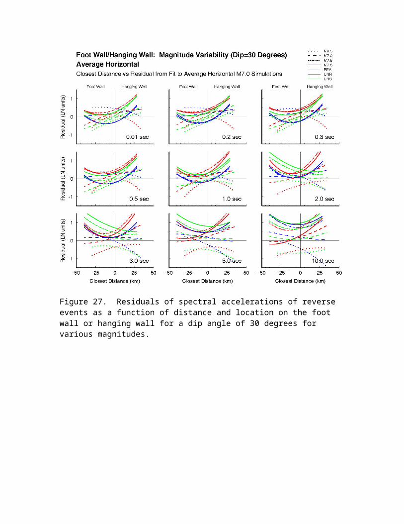
Figure 2. Magnitude scaling of spectral acceleration for strike-slip earthquakes assuming constant stress drop (top) and L model (bottom) scaling, normalized at M 7.
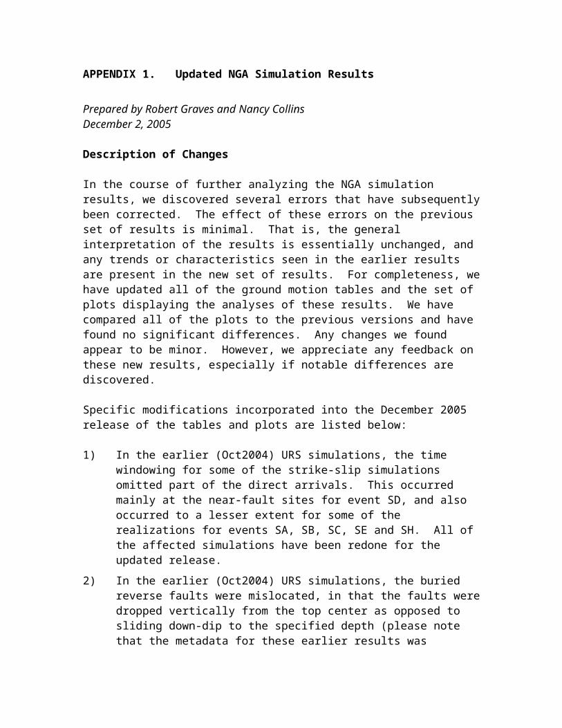
Figure 3. Shape of the acceleration response spectrum, normalized at 2 seconds period.
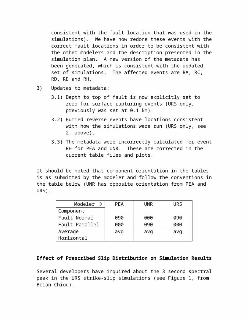
Figure 4. Residuals of spectral accelerations of strike-slip event SD as a function of the along strike directivity parameter X cos θ.
Figure 5. Residuals of spectral accelerations of M 7.5 strike-slip events as a function of rupture area (which is inversely related to static stress drop).
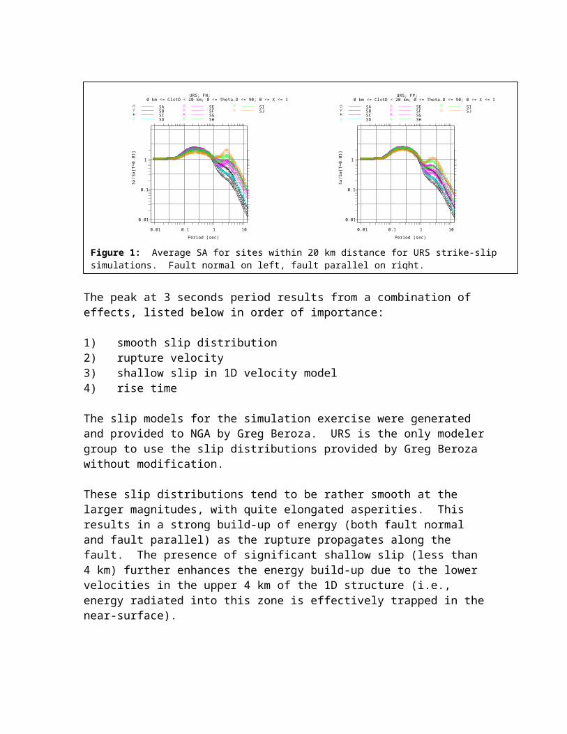
Figure 6. Residuals of spectral accelerations of M 6.5 reverse events as a function of depth to top of rupture.
Figure 7. Residuals of spectral accelerations of M 7 reverse event as a function of distance and location on the foot wall or hanging wall for various dip angle.