Embed Size (px)
Citation preview
© 2017 Fabio Pellacini and Steve Marschner • Computer Graphics
2D Spline Curves
1
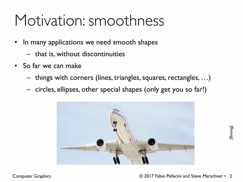
• In many applications we need smooth shapes
– that is, without discontinuities
• So far we can make
– things with corners (lines, triangles, squares, rectangles, …)
– circles, ellipses, other special shapes (only get you so far!)
© 2017 Fabio Pellacini and Steve Marschner • Computer Graphics
[Boe
ing]
Motivation: smoothness
2

• Pencil-and-paper draftsmen also needed smooth curves
• Origin of “spline:” strip of flexible metal
– held in place by pegs or weights to constrain shape
– traced to produce smooth contour
© 2017 Fabio Pellacini and Steve Marschner • Computer Graphics
Classical approach
3

• Smoothness
– in drafting spline, comes from physical curvature minimization
– in CG spline, comes from choosing smooth functions
• usually low-order polynomials
• Control
– in drafting spline, comes from fixed pegs
– in CG spline, comes from user-specified control points
© 2017 Fabio Pellacini and Steve Marschner • Computer Graphics
Translating into usable math
4
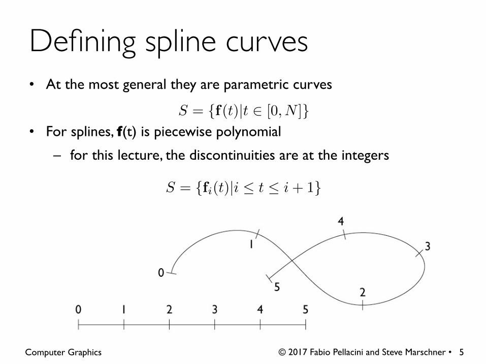
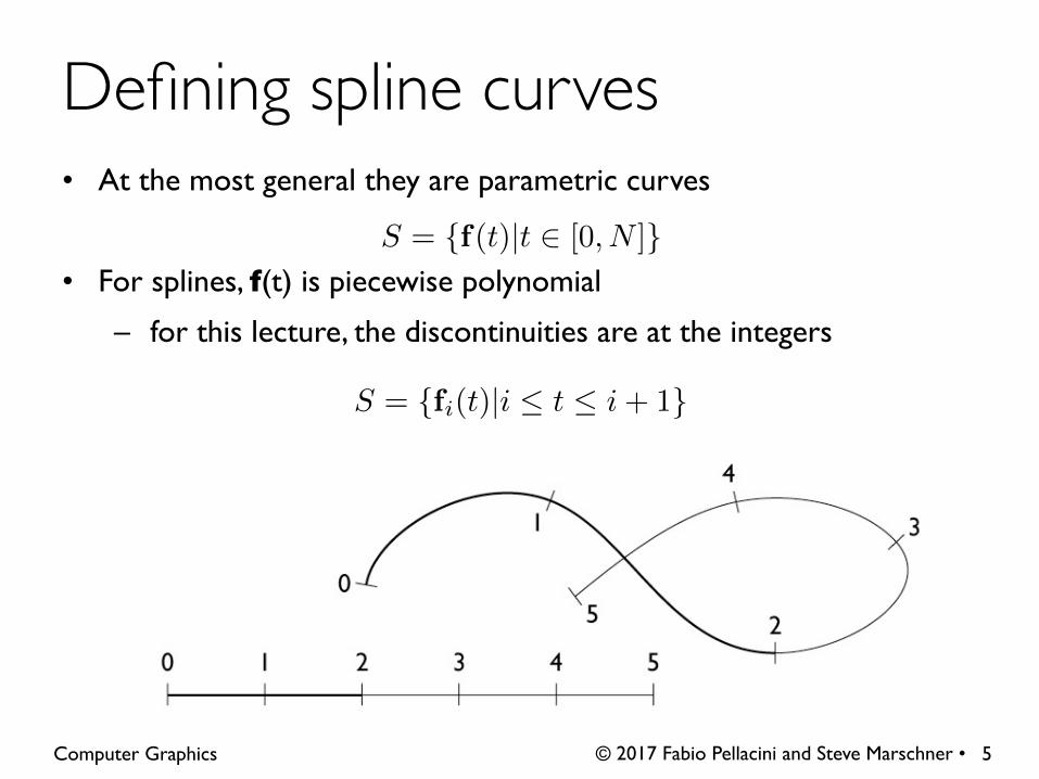
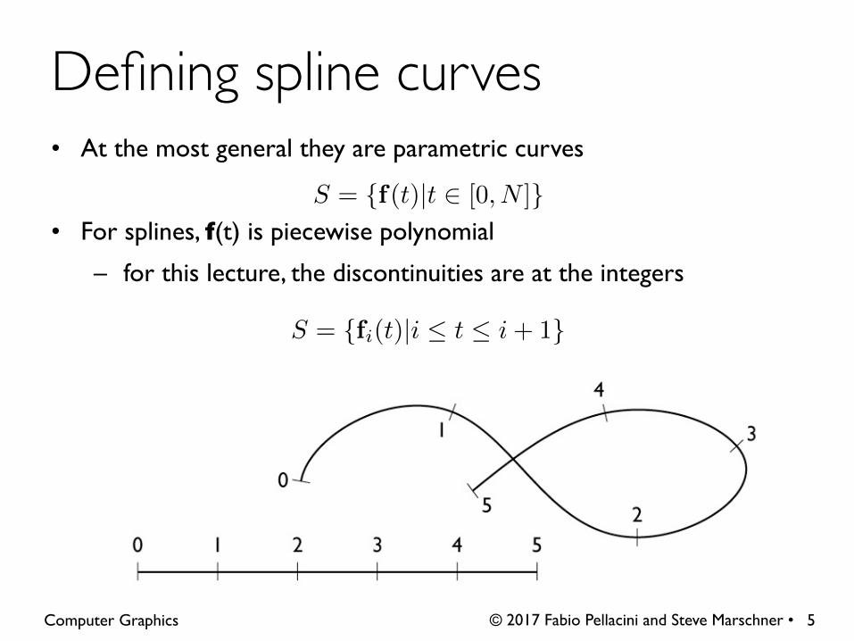
• At the most general they are parametric curves
• For splines, f(t) is piecewise polynomial
– for this lecture, the discontinuities are at the integers
© 2017 Fabio Pellacini and Steve Marschner • Computer Graphics
Defining spline curves
5
S = {fi(t)|i t i+ 1}
S = {f(t)|t 2 [0, N ]}

• At the most general they are parametric curves
• For splines, f(t) is piecewise polynomial
– for this lecture, the discontinuities are at the integers
© 2017 Fabio Pellacini and Steve Marschner • Computer Graphics
Defining spline curves
5
S = {fi(t)|i t i+ 1}
S = {f(t)|t 2 [0, N ]}
• At the most general they are parametric curves
• For splines, f(t) is piecewise polynomial
– for this lecture, the discontinuities are at the integers
© 2017 Fabio Pellacini and Steve Marschner • Computer Graphics
Defining spline curves
5
S = {fi(t)|i t i+ 1}
S = {f(t)|t 2 [0, N ]}
• At the most general they are parametric curves
• For splines, f(t) is piecewise polynomial
– for this lecture, the discontinuities are at the integers
© 2017 Fabio Pellacini and Steve Marschner • Computer Graphics
Defining spline curves
5
S = {fi(t)|i t i+ 1}
S = {f(t)|t 2 [0, N ]}

• f(t) is a piecewise polynomial
– for this lecture, the discontinuities are at the integers
• Example: a cubic spline has the following form over [i, i+1):
• Vector notation
• Coefficients are different for every interval
© 2017 Fabio Pellacini and Steve Marschner • Computer Graphics
Defining spline curves
6
p(t) = at3 + bt2 + ct+ d
x(t) = axt3 + bxt
2 + cxt+ dx
y(t) = ayt3 + byt
2 + cyt+ dy
p(t) = ai(t� i)3 + bi(t� i)2 + ci(t� i) + di
t 2 [0, N), i 2 {0, 1, 2, 3, ...}
t 2 [0, 1)
t 2 [0, 1)

© 2017 Fabio Pellacini and Steve Marschner • Computer Graphics
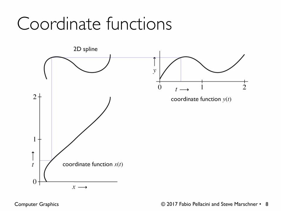
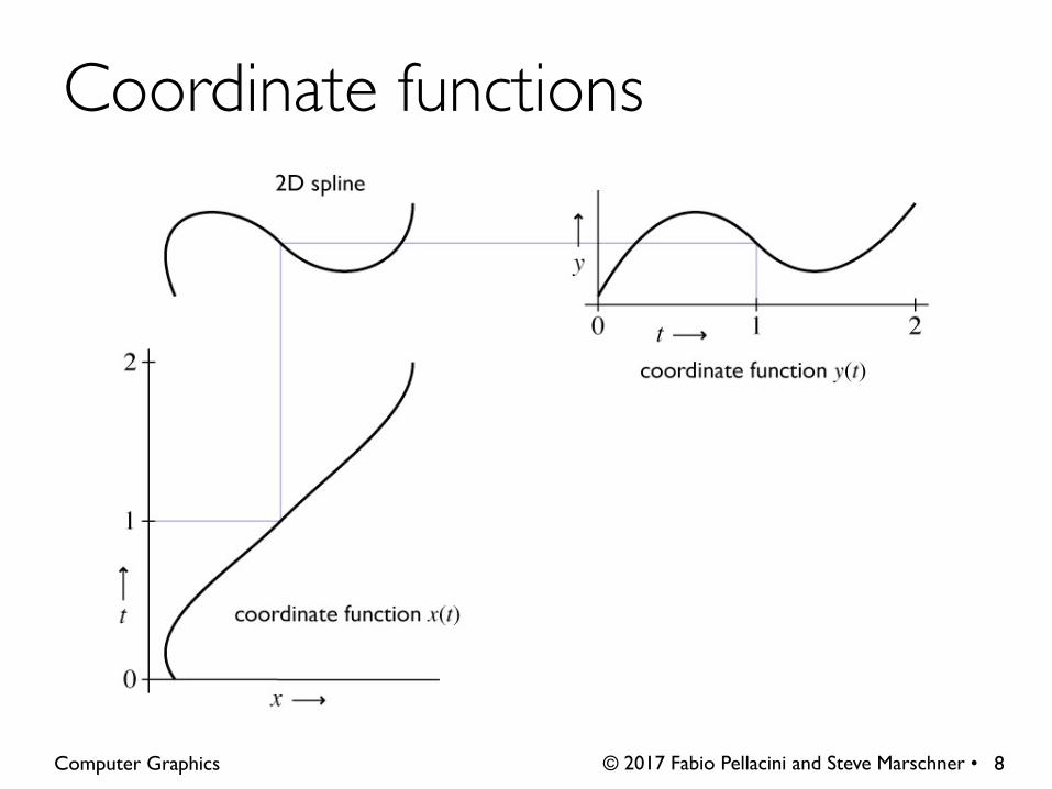
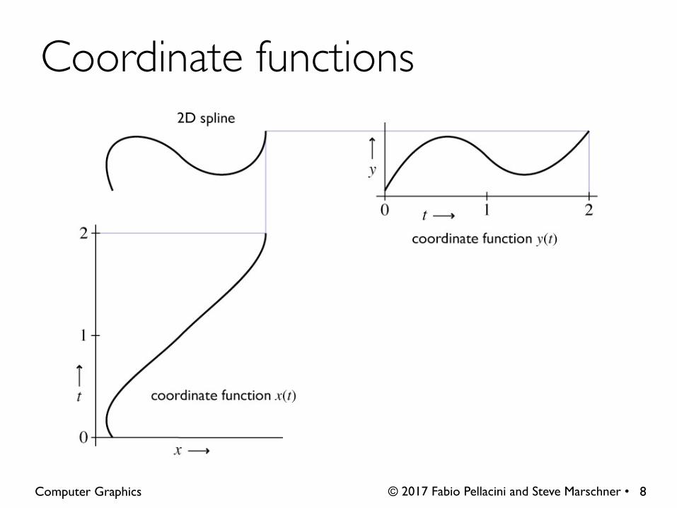
Coordinate functions
7
© 2017 Fabio Pellacini and Steve Marschner • Computer Graphics
Coordinate functions
7

© 2017 Fabio Pellacini and Steve Marschner • Computer Graphics
Coordinate functions
7

© 2017 Fabio Pellacini and Steve Marschner • Computer Graphics
Coordinate functions
7
© 2017 Fabio Pellacini and Steve Marschner • Computer Graphics
Coordinate functions
8
© 2017 Fabio Pellacini and Steve Marschner • Computer Graphics
Coordinate functions
8
© 2017 Fabio Pellacini and Steve Marschner • Computer Graphics
Coordinate functions
8
© 2017 Fabio Pellacini and Steve Marschner • Computer Graphics
Coordinate functions
8
© 2017 Fabio Pellacini and Steve Marschner • Computer Graphics
Coordinate functions
8
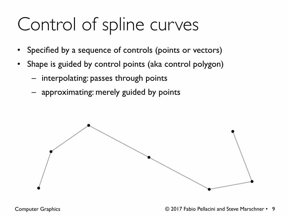
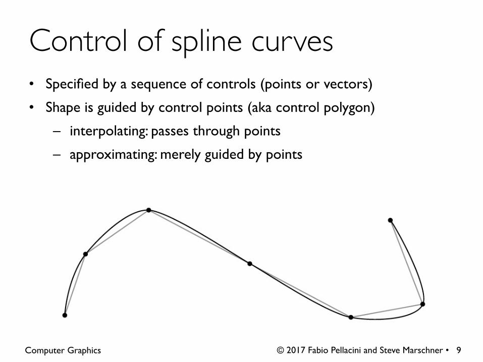
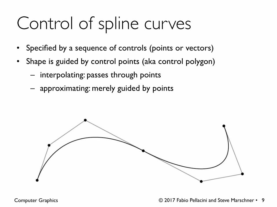
• Specified by a sequence of controls (points or vectors)
• Shape is guided by control points (aka control polygon)
– interpolating: passes through points
– approximating: merely guided by points
© 2017 Fabio Pellacini and Steve Marschner • Computer Graphics
Control of spline curves
9
• Specified by a sequence of controls (points or vectors)
• Shape is guided by control points (aka control polygon)
– interpolating: passes through points
– approximating: merely guided by points
© 2017 Fabio Pellacini and Steve Marschner • Computer Graphics
Control of spline curves
9

• Specified by a sequence of controls (points or vectors)
• Shape is guided by control points (aka control polygon)
– interpolating: passes through points
– approximating: merely guided by points
© 2017 Fabio Pellacini and Steve Marschner • Computer Graphics
Control of spline curves
9
• Specified by a sequence of controls (points or vectors)
• Shape is guided by control points (aka control polygon)
– interpolating: passes through points
– approximating: merely guided by points
© 2017 Fabio Pellacini and Steve Marschner • Computer Graphics
Control of spline curves
9
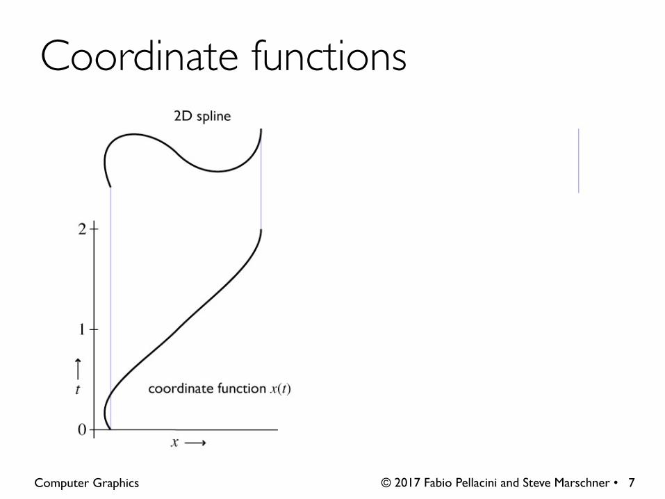
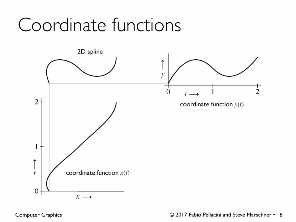
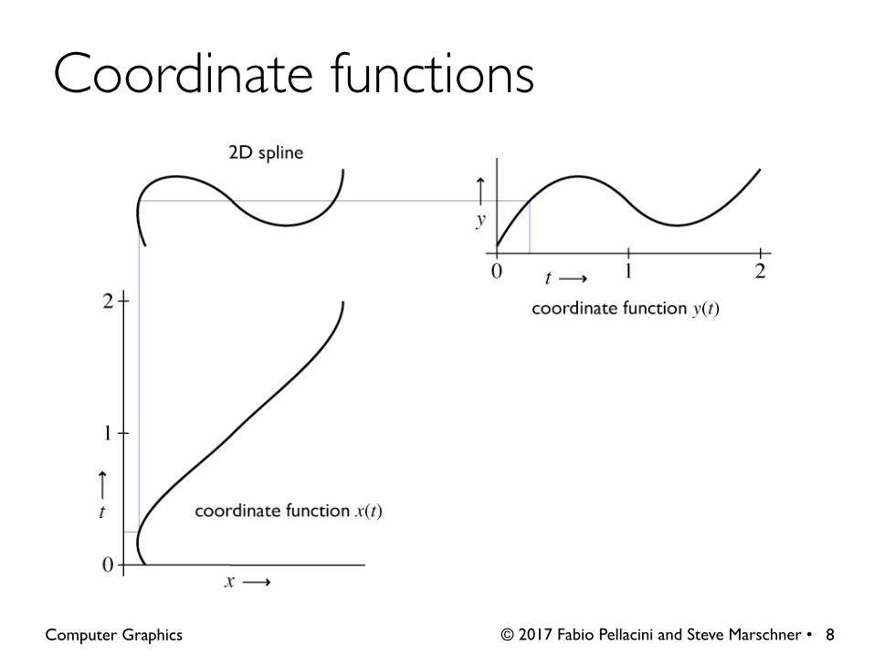
• Each coordinate is separate
– the function x(t) is determined solely by the x coordinates of the control points
– this means 1D, 2D, 3D, … curves are all really the same
• Spline curves are linear functions of their controls
– moving a control point two inches to the right moves x(t) twice as far as moving it by one inch
– x(t), for fixed t, is a linear combination (weighted sum) of the controls’ x coordinates
– f(t), for fixed t, is a linear combination (weighted sum) of the controls
© 2017 Fabio Pellacini and Steve Marschner • Computer Graphics
Splines and control points
10
• Spline segments: how to define a polynomial on [0,1]
– that has the properties you want and is easy to control
• Spline curves: how to chain together segments
– so that the whole curve has the properties you want and is easy to control
• Refinement: how to add detail to splines
• Evaluation: how to approximate them with line segments
© 2017 Fabio Pellacini and Steve Marschner • Computer Graphics
Designing spline curves
11

© 2017 Fabio Pellacini and Steve Marschner • Computer Graphics
Spline Segments
12
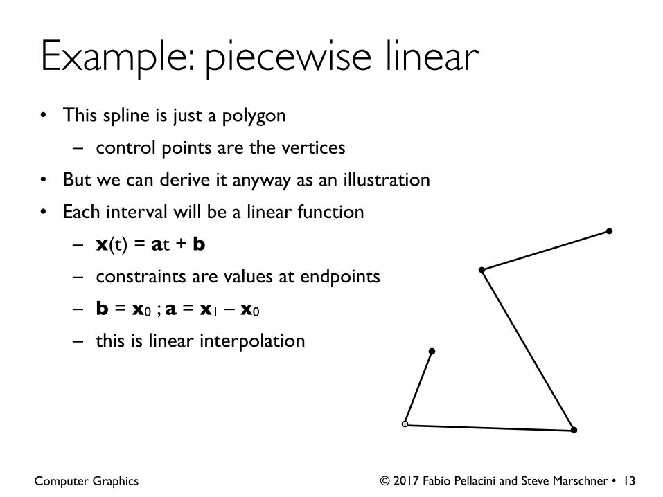
• This spline is just a polygon
– control points are the vertices
• But we can derive it anyway as an illustration
• Each interval will be a linear function
– x(t) = at + b– constraints are values at endpoints
– b = x0 ; a = x1 – x0
– this is linear interpolation
© 2017 Fabio Pellacini and Steve Marschner • Computer Graphics
Example: piecewise linear
13
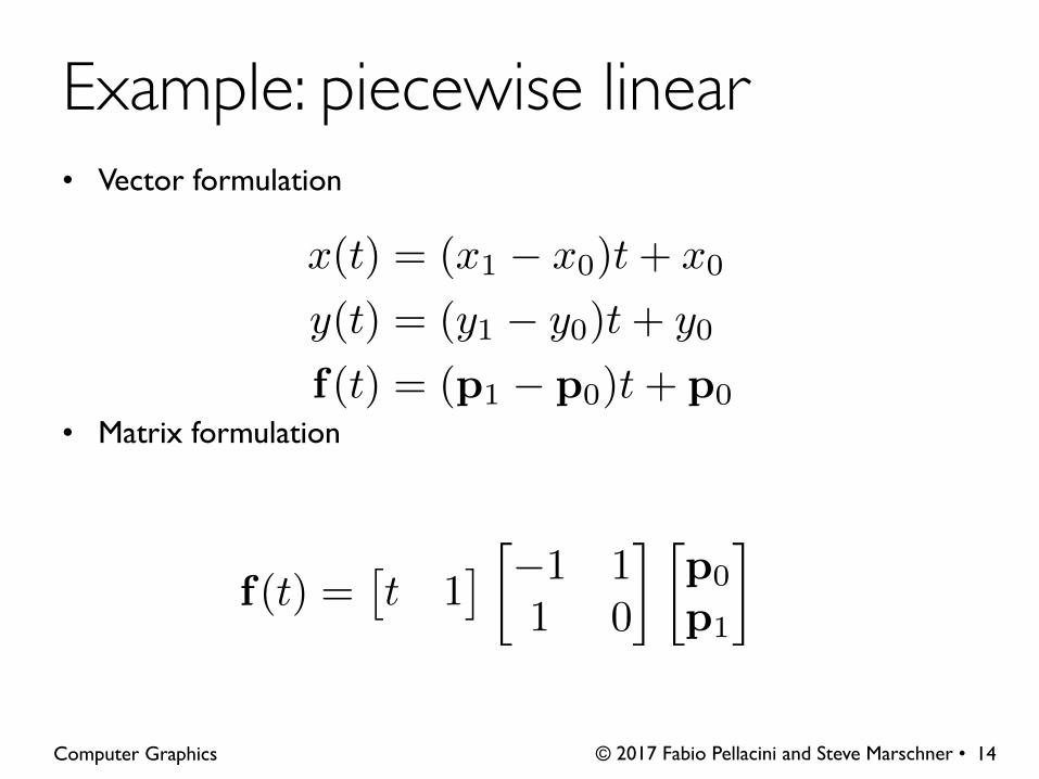
• Vector formulation
• Matrix formulation
© 2017 Fabio Pellacini and Steve Marschner • Computer Graphics
Example: piecewise linear
14
f(t) =⇥t 1
⇤ �1 11 0
� p0
p1
�
x(t) = (x1 � x0)t+ x0
y(t) = (y1 � y0)t+ y0
f(t) = (p1 � p0)t+ p0

• Basis function formulation
– regroup expression by p rather than t
– interpretation in matrix viewpoint
© 2017 Fabio Pellacini and Steve Marschner • Computer Graphics
Example: piecewise linear
15
f(t) = (p1 � p0)t+ p0
= (1� t)p0 + tp1
f(t) =
✓⇥t 1
⇤ �1 11 0
�◆p0
p1
�

• Vector blending formulation: “average of points”
– blending functions: contribution of each point as t changes
© 2017 Fabio Pellacini and Steve Marschner • Computer Graphics
Example: piecewise linear
16
b0(t) = 1� t b1(t) = t
t
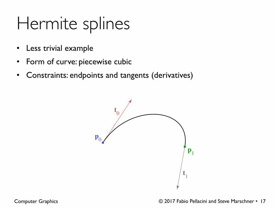
• Less trivial example
• Form of curve: piecewise cubic
• Constraints: endpoints and tangents (derivatives)
© 2017 Fabio Pellacini and Steve Marschner • Computer Graphics
Hermite splines
17
t0
p1
p0
t1
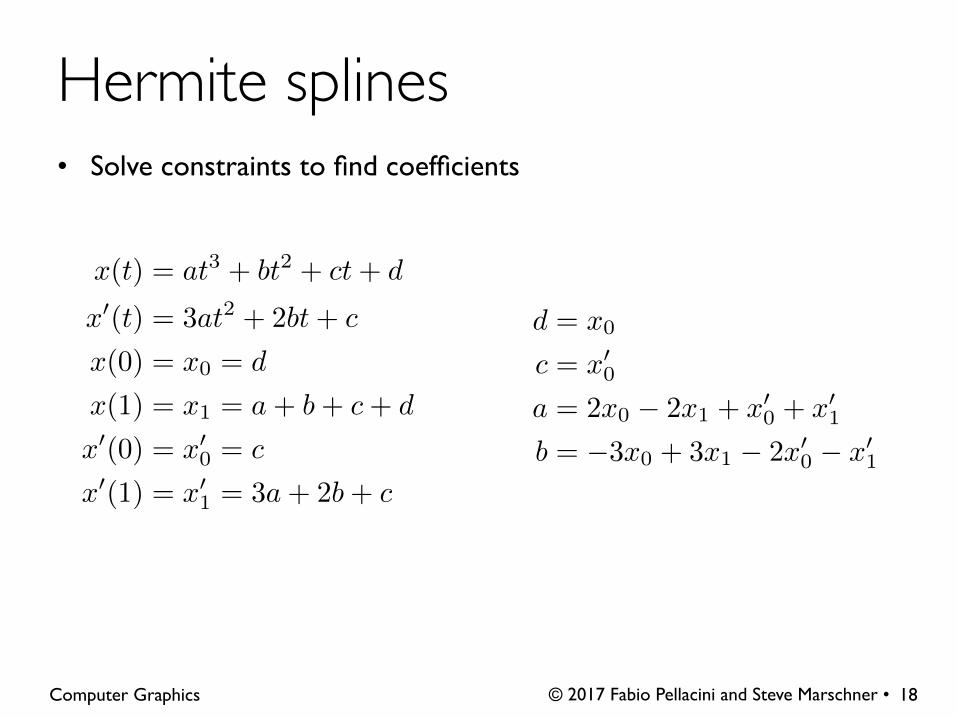
• Solve constraints to find coefficients
© 2017 Fabio Pellacini and Steve Marschner • Computer Graphics
Hermite splines
18
x(t) = at3 + bt2 + ct+ d
x0(t) = 3at2 + 2bt+ c
x(0) = x0 = d
x(1) = x1 = a+ b+ c+ d
x0(0) = x00 = c
x0(1) = x01 = 3a+ 2b+ c
d = x0
c = x00
a = 2x0 � 2x1 + x00 + x0
1
b = �3x0 + 3x1 � 2x00 � x0
1

© 2017 Fabio Pellacini and Steve Marschner • Computer Graphics
Matrix form of spline
19
⇥t3 t2 t 1
⇤
2
664
⇥ ⇥ ⇥ ⇥⇥ ⇥ ⇥ ⇥⇥ ⇥ ⇥ ⇥⇥ ⇥ ⇥ ⇥
3
775
2
664
p0
p1
p2
p3
3
775
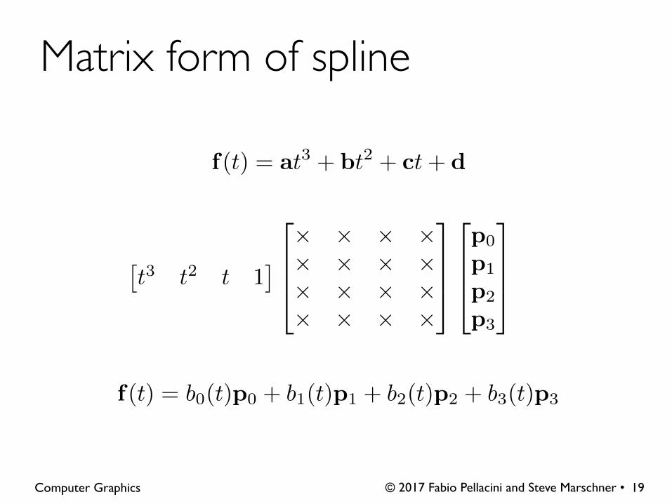
f(t) = b0(t)p0 + b1(t)p1 + b2(t)p2 + b3(t)p3
f(t) = at3 + bt2 + ct+ d

© 2017 Fabio Pellacini and Steve Marschner • Computer Graphics
Matrix form of spline
19
⇥t3 t2 t 1
⇤
2
664
⇥ ⇥ ⇥ ⇥⇥ ⇥ ⇥ ⇥⇥ ⇥ ⇥ ⇥⇥ ⇥ ⇥ ⇥
3
775
2
664
p0
p1
p2
p3
3
775
f(t) = b0(t)p0 + b1(t)p1 + b2(t)p2 + b3(t)p3
f(t) = at3 + bt2 + ct+ d
© 2017 Fabio Pellacini and Steve Marschner • Computer Graphics
Matrix form of spline
19
⇥t3 t2 t 1
⇤
2
664
⇥ ⇥ ⇥ ⇥⇥ ⇥ ⇥ ⇥⇥ ⇥ ⇥ ⇥⇥ ⇥ ⇥ ⇥
3
775
2
664
p0
p1
p2
p3
3
775
f(t) = b0(t)p0 + b1(t)p1 + b2(t)p2 + b3(t)p3
f(t) = at3 + bt2 + ct+ d

© 2017 Fabio Pellacini and Steve Marschner • Computer Graphics
Matrix form of spline
19
⇥t3 t2 t 1
⇤
2
664
⇥ ⇥ ⇥ ⇥⇥ ⇥ ⇥ ⇥⇥ ⇥ ⇥ ⇥⇥ ⇥ ⇥ ⇥
3
775
2
664
p0
p1
p2
p3
3
775
f(t) = b0(t)p0 + b1(t)p1 + b2(t)p2 + b3(t)p3
f(t) = at3 + bt2 + ct+ d
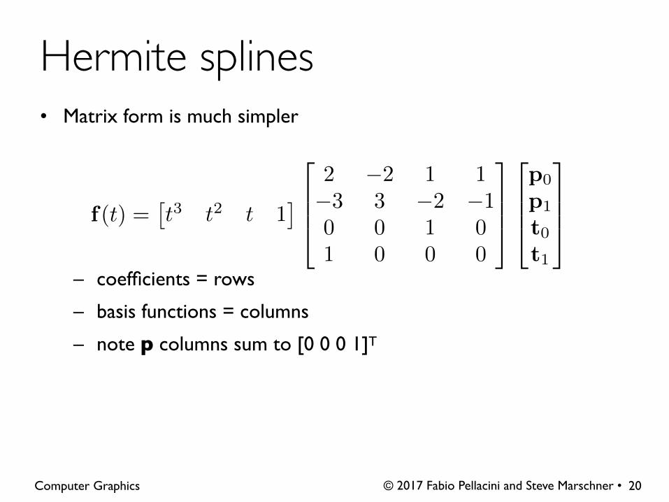
• Matrix form is much simpler
– coefficients = rows
– basis functions = columns
– note p columns sum to [0 0 0 1]T
© 2017 Fabio Pellacini and Steve Marschner • Computer Graphics
Hermite splines
20
f(t) =⇥t3 t2 t 1
⇤
2
664
2 �2 1 1�3 3 �2 �10 0 1 01 0 0 0
3
775
2
664
p0
p1
t0t1
3
775
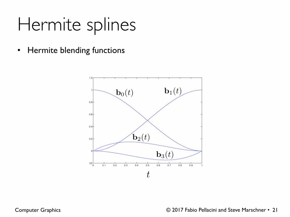
• Hermite blending functions
© 2017 Fabio Pellacini and Steve Marschner • Computer Graphics
Hermite splines
21
t
b2(t)
b3(t)
b0(t) b1(t)

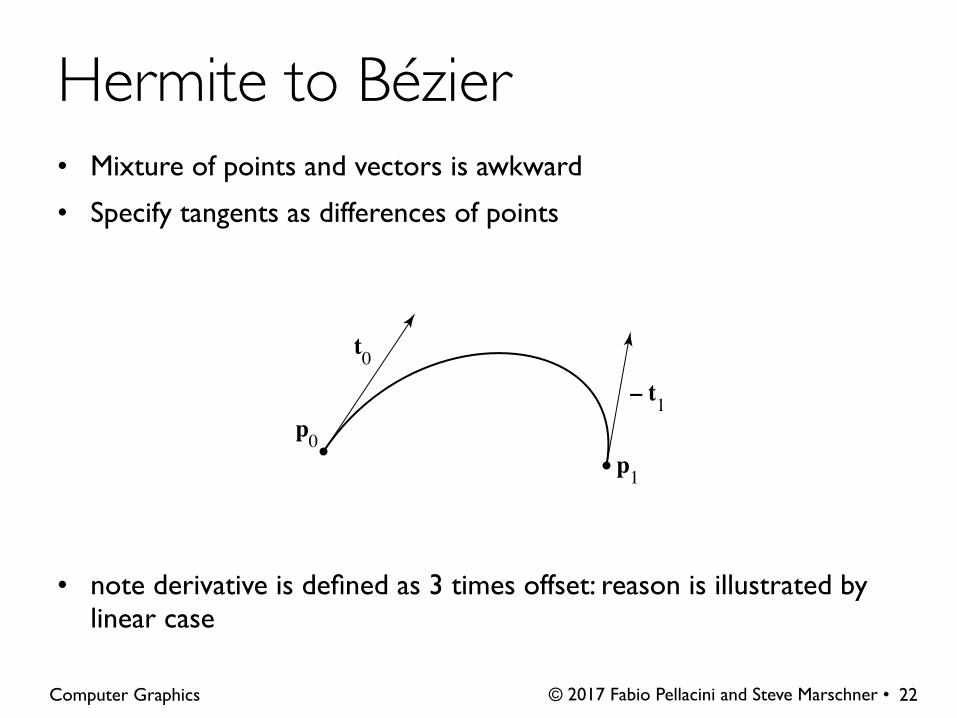
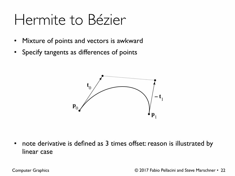
• Mixture of points and vectors is awkward
• Specify tangents as differences of points
• note derivative is defined as 3 times offset: reason is illustrated by linear case
© 2017 Fabio Pellacini and Steve Marschner • Computer Graphics
Hermite to Bézier
22
p0
t0
p1
t1
• Mixture of points and vectors is awkward
• Specify tangents as differences of points
• note derivative is defined as 3 times offset: reason is illustrated by linear case
© 2017 Fabio Pellacini and Steve Marschner • Computer Graphics
Hermite to Bézier
22
p0
t0
p1
– t1
• Mixture of points and vectors is awkward
• Specify tangents as differences of points
• note derivative is defined as 3 times offset: reason is illustrated by linear case
© 2017 Fabio Pellacini and Steve Marschner • Computer Graphics
Hermite to Bézier
22
p0
t0
p1
– t1

• Mixture of points and vectors is awkward
• Specify tangents as differences of points
• note derivative is defined as 3 times offset: reason is illustrated by linear case
© 2017 Fabio Pellacini and Steve Marschner • Computer Graphics
Hermite to Bézier
22
p0
t0
p1
– t1
q0
q1 q2
q3
I’m calling these points q just for this slide and the
next one.
© 2017 Fabio Pellacini and Steve Marschner • Computer Graphics
Hermite to Bézier
23
p0
t0
p1
– t1
q0
q1 q2
q3
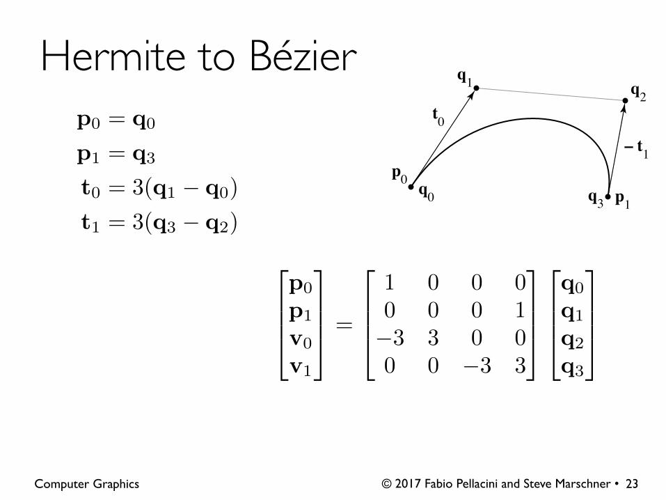
p0 = q0
p1 = q3
t0 = 3(q1 � q0)
t1 = 3(q3 � q2)
2
664
p0
p1
v0
v1
3
775 =
2
664
1 0 0 00 0 0 1�3 3 0 00 0 �3 3
3
775
2
664
q0
q1
q2
q3
3
775

© 2017 Fabio Pellacini and Steve Marschner • Computer Graphics
Hermite to Bézier
24
p0
t0
p1
– t1
q0
q1 q2
q3
p0 = q0
p1 = q3
t0 = 3(q1 � q0)
t1 = 3(q3 � q2)
2
664
abcd
3
775 =
2
664
2 �2 1 1�3 3 �2 �10 0 1 01 0 0 0
3
775
2
664
1 0 0 00 0 0 1�3 3 0 00 0 �3 3
3
775
2
664
q0
q1
q2
q3
3
775
© 2017 Fabio Pellacini and Steve Marschner • Computer Graphics
Hermite to Bézier
25
p0
t0
p1
– t1
q0
q1 q2
q3
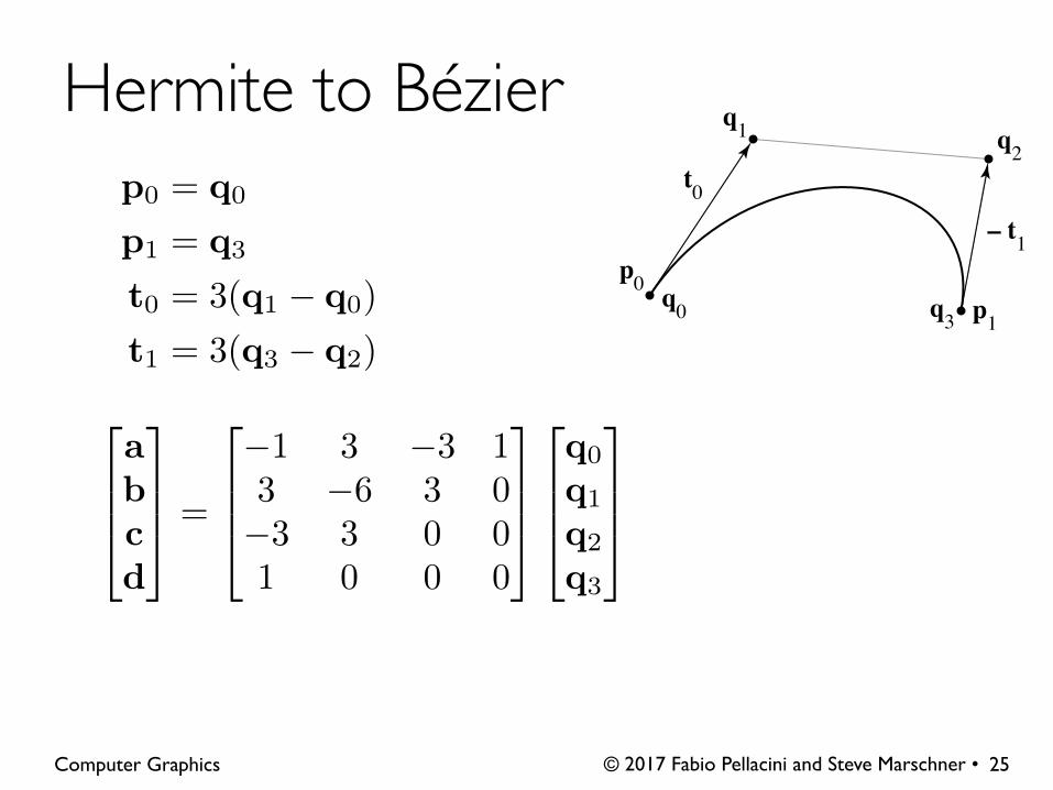
p0 = q0
p1 = q3
t0 = 3(q1 � q0)
t1 = 3(q3 � q2)
2
664
abcd
3
775 =
2
664
�1 3 �3 13 �6 3 0�3 3 0 01 0 0 0
3
775
2
664
q0
q1
q2
q3
3
775
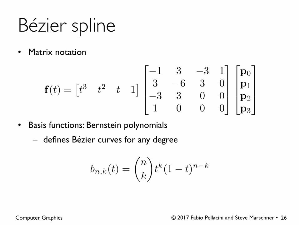
• Matrix notation
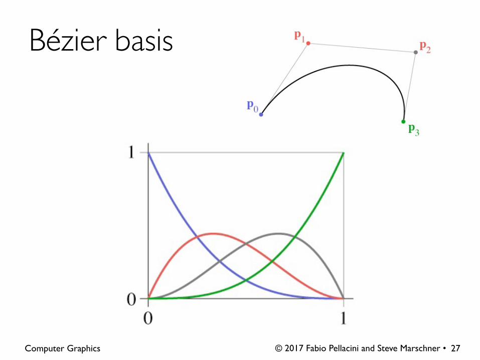
• Basis functions: Bernstein polynomials
– defines Bézier curves for any degree
© 2017 Fabio Pellacini and Steve Marschner • Computer Graphics
Bézier spline
26
f(t) =⇥t3 t2 t 1
⇤
2
664
�1 3 �3 13 �6 3 0�3 3 0 01 0 0 0
3
775
2
664
p0
p1
p2
p3
3
775
bn,k(t) =
✓n
k
◆tk(1� t)n�k
© 2017 Fabio Pellacini and Steve Marschner • Computer Graphics
Bézier basis
27
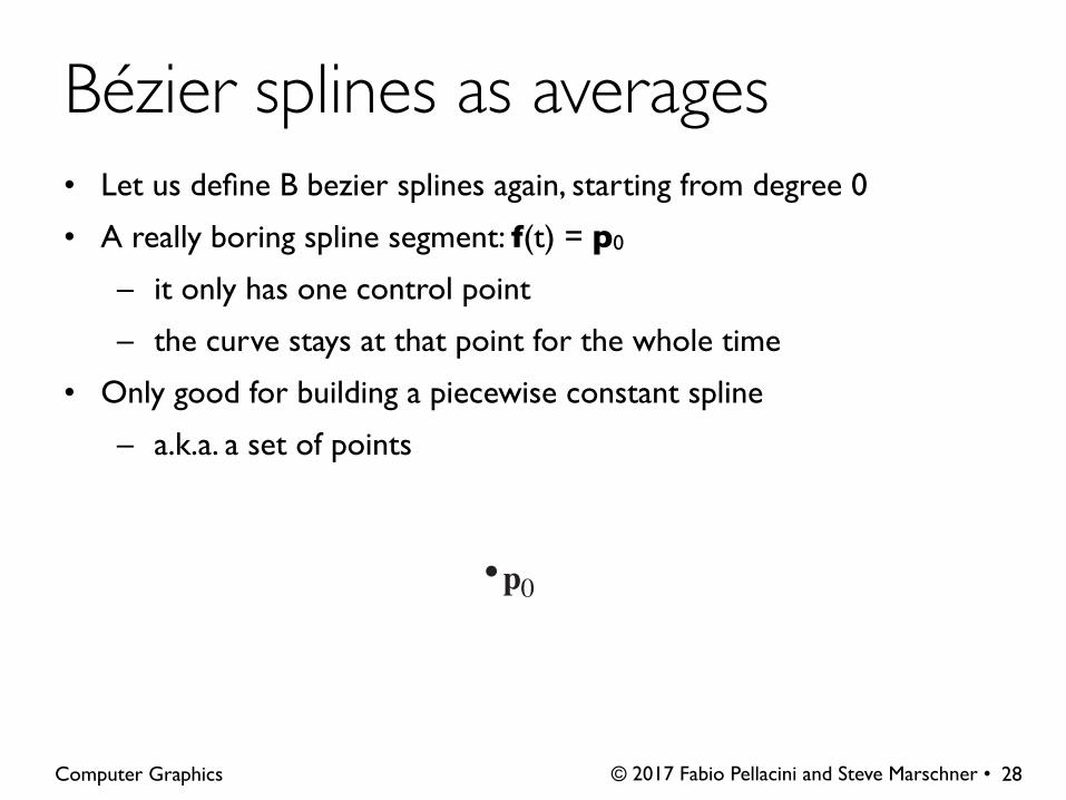
• Let us define B bezier splines again, starting from degree 0
• A really boring spline segment: f(t) = p0
– it only has one control point
– the curve stays at that point for the whole time
• Only good for building a piecewise constant spline
– a.k.a. a set of points
© 2017 Fabio Pellacini and Steve Marschner • Computer Graphics
Bézier splines as averages
28
p0

• A piecewise linear spline segment
– two control points per segment
– blend them with weights α and β = 1 – α– α and β are weights not distances
• Good for building a piecewise linear spline
– a.k.a. a polygon or polyline
© 2017 Fabio Pellacini and Steve Marschner • Computer Graphics
Bézier splines as averages
29
α
β
p0
αp0 + βp1
p1
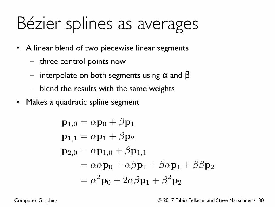
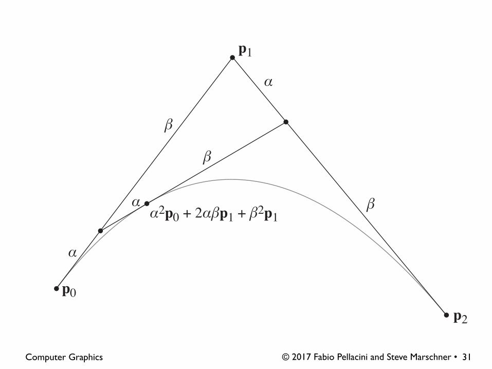
• A linear blend of two piecewise linear segments
– three control points now
– interpolate on both segments using α and β– blend the results with the same weights
• Makes a quadratic spline segment
© 2017 Fabio Pellacini and Steve Marschner • Computer Graphics
Bézier splines as averages
30
p1,0 = ↵p0 + �p1
p1,1 = ↵p1 + �p2
p2,0 = ↵p1,0 + �p1,1
= ↵↵p0 + ↵�p1 + �↵p1 + ��p2
= ↵2p0 + 2↵�p1 + �2p2
© 2017 Fabio Pellacini and Steve Marschner • Computer Graphics 31
α
α
α
β
β
β
α2p0 + 2αβp1 + β2p1
p0
p2
p1
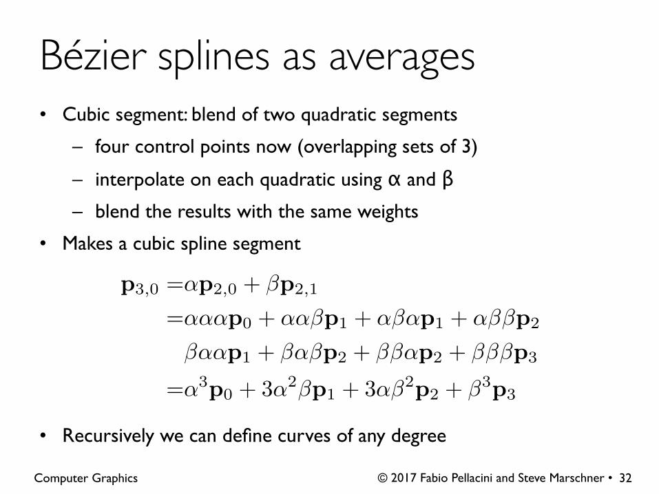
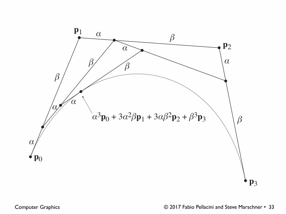
• Cubic segment: blend of two quadratic segments
– four control points now (overlapping sets of 3)
– interpolate on each quadratic using α and β– blend the results with the same weights
• Makes a cubic spline segment
• Recursively we can define curves of any degree
© 2017 Fabio Pellacini and Steve Marschner • Computer Graphics
Bézier splines as averages
32
p3,0 =↵p2,0 + �p2,1
=↵↵↵p0 + ↵↵�p1 + ↵�↵p1 + ↵��p2
�↵↵p1 + �↵�p2 + ��↵p2 + ���p3
=↵3p0 + 3↵2�p1 + 3↵�2p2 + �3p3
© 2017 Fabio Pellacini and Steve Marschner • Computer Graphics 33
α
α α
αα
α
β
β
β
ββ
α3p0 + 3α2βp1 + 3αβ2p2 + β3p3
p0
p2
p3
p1
© 2017 Fabio Pellacini and Steve Marschner • Computer Graphics
Bézier spline
34
[Wik
iped
iaC
omm
ons]

© 2017 Fabio Pellacini and Steve Marschner • Computer Graphics
Bézier spline
34
[Wik
iped
iaC
omm
ons]
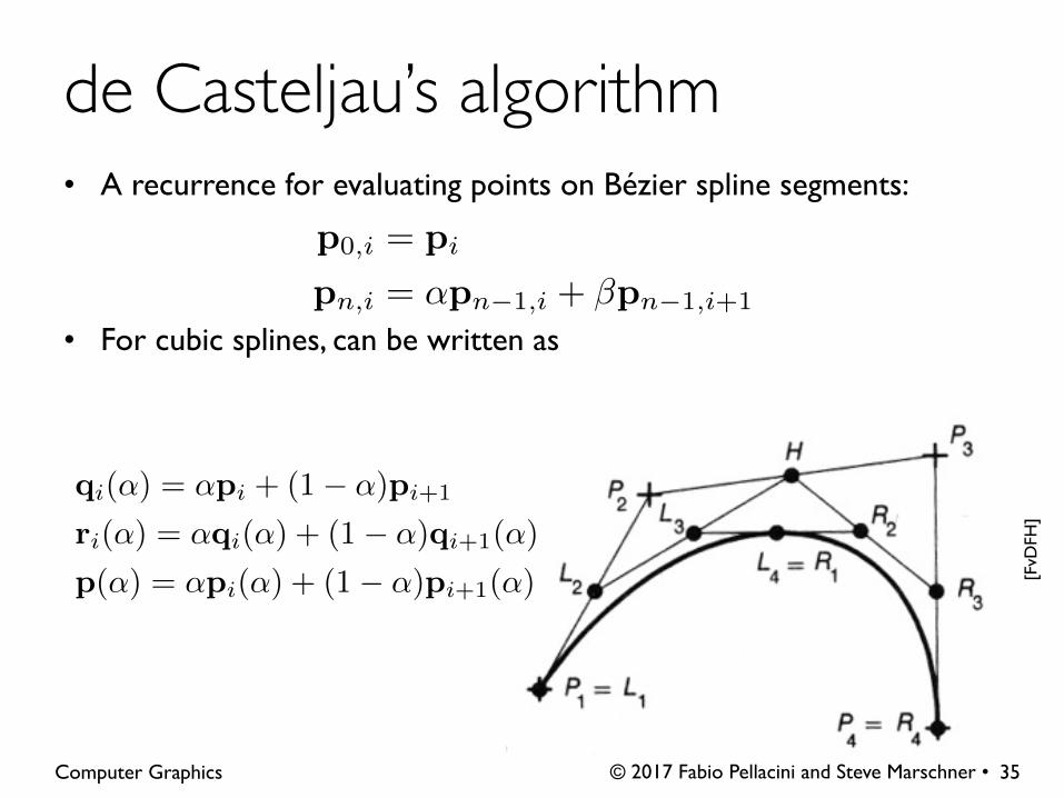
• A recurrence for evaluating points on Bézier spline segments:
• For cubic splines, can be written as
© 2017 Fabio Pellacini and Steve Marschner • Computer Graphics
[FvD
FH]
de Casteljau’s algorithm
35
p0,i = pi
pn,i = ↵pn�1,i + �pn�1,i+1
qi(↵) = ↵pi + (1� ↵)pi+1
ri(↵) = ↵qi(↵) + (1� ↵)qi+1(↵)
p(↵) = ↵pi(↵) + (1� ↵)pi+1(↵)

• Very widely used type, especially in 2D
– e.g. it is a primitive in PostScript/PDF
• Can represent smooth curves with corners
• Nice de Casteljau recurrence for evaluation
• Can easily add points at any position
© 2017 Fabio Pellacini and Steve Marschner • Computer Graphics
Cubic Bézier splines
36
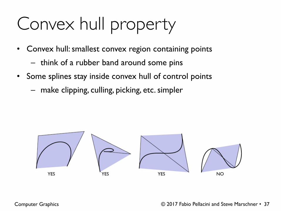
• Convex hull: smallest convex region containing points
– think of a rubber band around some pins
• Some splines stay inside convex hull of control points
– make clipping, culling, picking, etc. simpler
© 2017 Fabio Pellacini and Steve Marschner • Computer Graphics
YES YES YES NO
Convex hull property
37

• If basis functions are all positive, the spline has the convex hull property
– we’re still requiring them to sum to 1
• If any basis function is ever negative, no convex hull prop.
– proof: take the other three points at the same place
© 2017 Fabio Pellacini and Steve Marschner • Computer Graphics
Convex hull properties
38

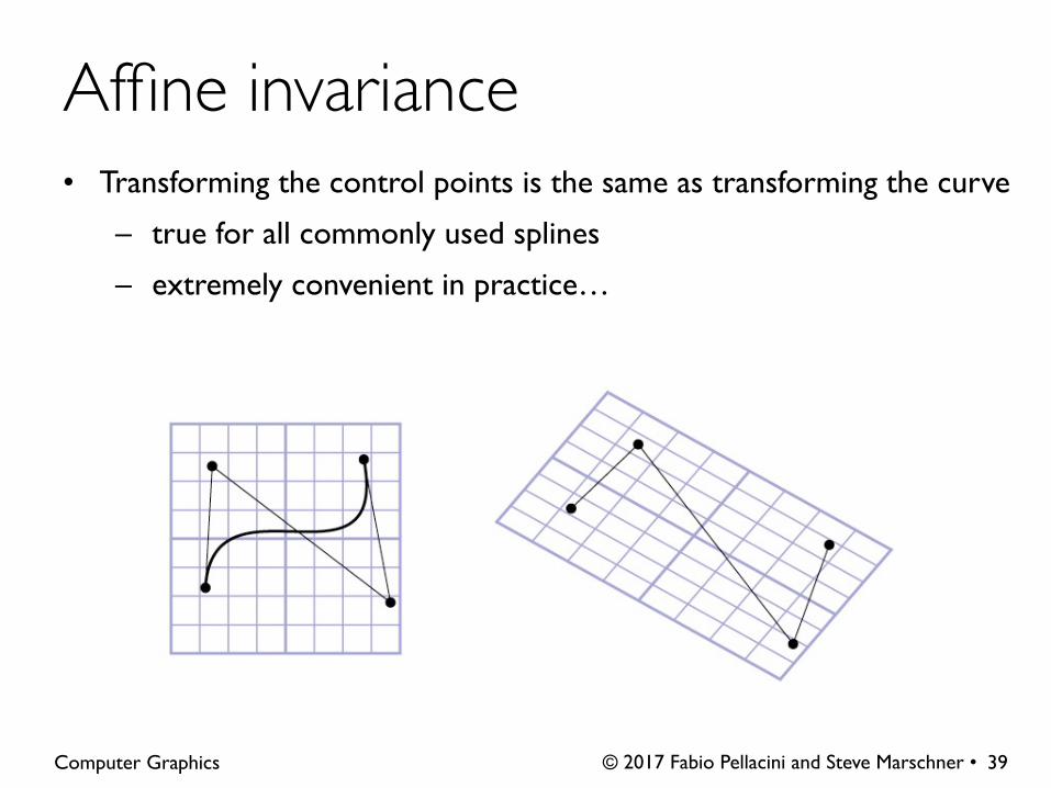
• Transforming the control points is the same as transforming the curve
– true for all commonly used splines
– extremely convenient in practice…
© 2017 Fabio Pellacini and Steve Marschner • Computer Graphics
Affine invariance
39
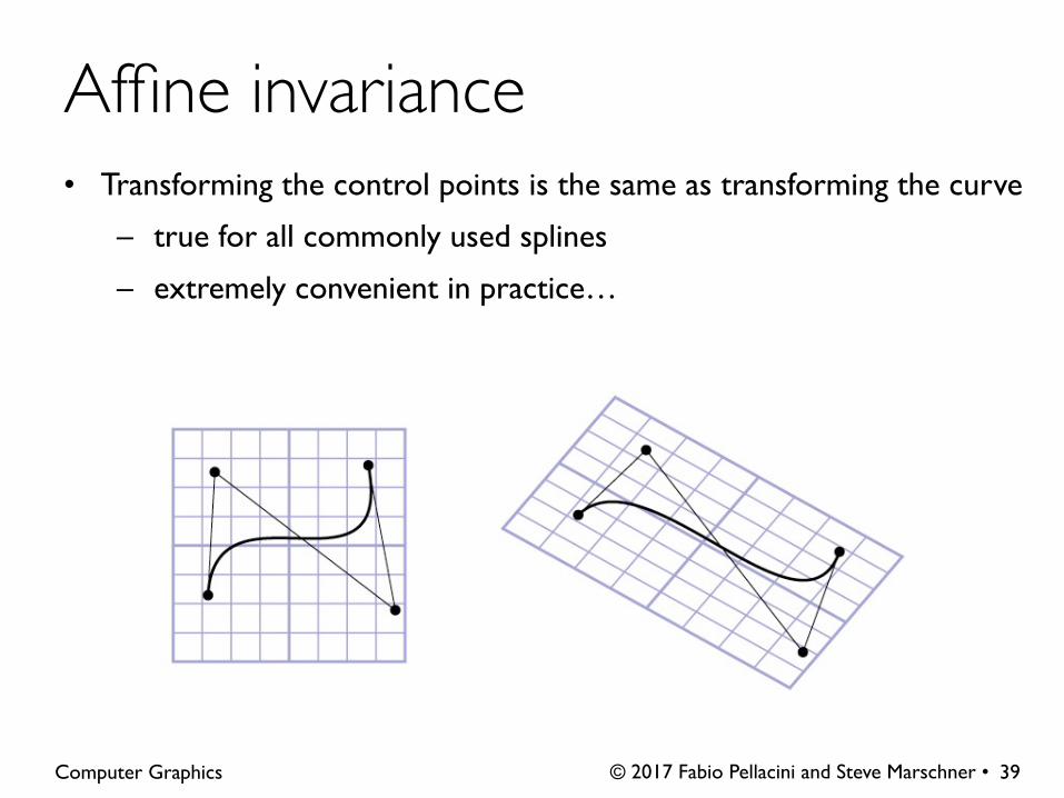
• Transforming the control points is the same as transforming the curve
– true for all commonly used splines
– extremely convenient in practice…
© 2017 Fabio Pellacini and Steve Marschner • Computer Graphics
Affine invariance
39
• Transforming the control points is the same as transforming the curve
– true for all commonly used splines
– extremely convenient in practice…
© 2017 Fabio Pellacini and Steve Marschner • Computer Graphics
Affine invariance
39
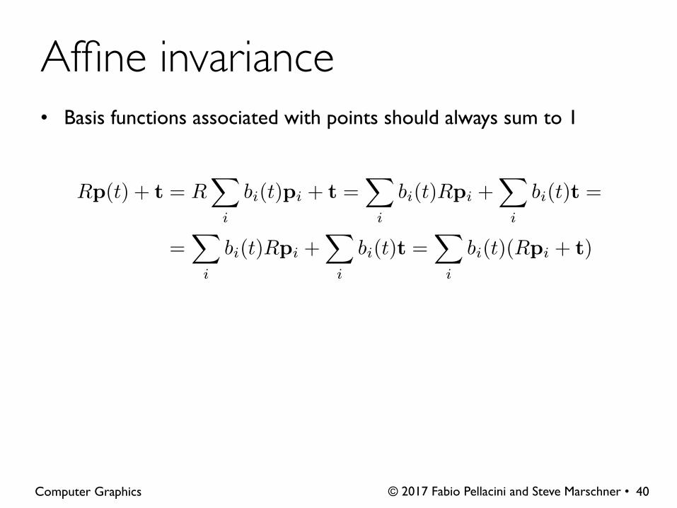
• Basis functions associated with points should always sum to 1
© 2017 Fabio Pellacini and Steve Marschner • Computer Graphics
Affine invariance
40
Rp(t) + t = RX
i
bi(t)pi + t =X
i
bi(t)Rpi +X
i
bi(t)t =
=X
i
bi(t)Rpi +X
i
bi(t)t =X
i
bi(t)(Rpi + t)

© 2017 Fabio Pellacini and Steve Marschner • Computer Graphics
Spline Curves
41
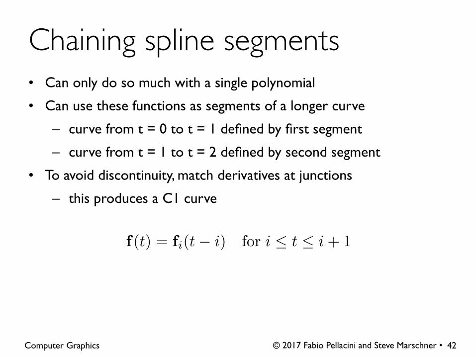
• Can only do so much with a single polynomial
• Can use these functions as segments of a longer curve
– curve from t = 0 to t = 1 defined by first segment
– curve from t = 1 to t = 2 defined by second segment
• To avoid discontinuity, match derivatives at junctions
– this produces a C1 curve
© 2017 Fabio Pellacini and Steve Marschner • Computer Graphics
Chaining spline segments
42
f(t) = fi(t� i) for i t i+ 1

• Changing control point only affects a limited part of spline
• Without this, splines are very difficult to use
• Many likely formulations lack this
– natural spline
– polynomial fits
© 2017 Fabio Pellacini and Steve Marschner • Computer Graphics
Local control
43

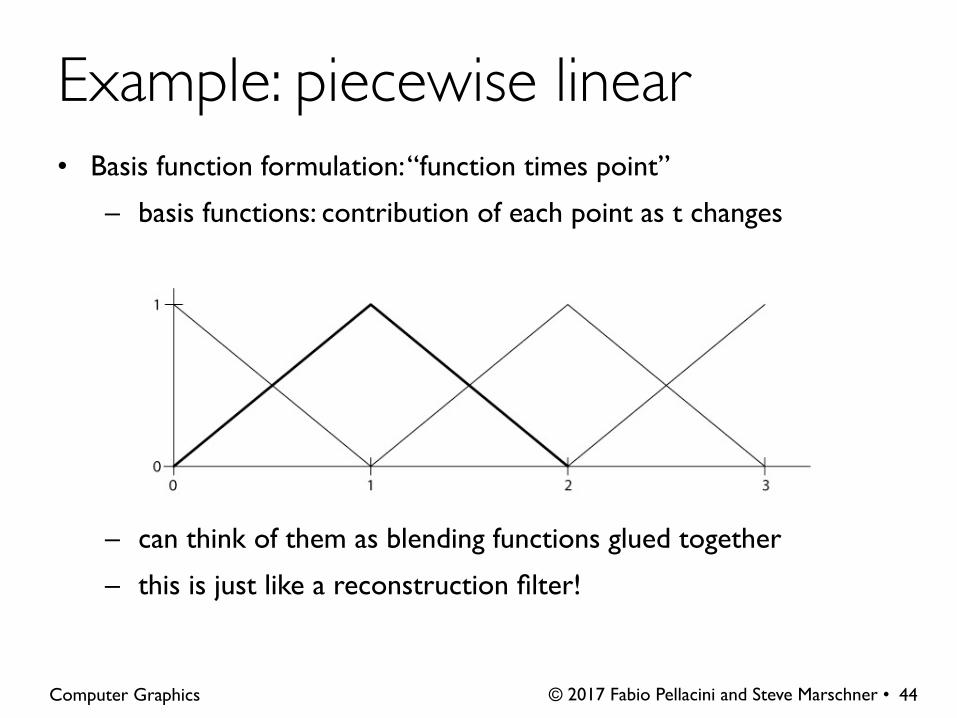
• Basis function formulation: “function times point”
– basis functions: contribution of each point as t changes
– can think of them as blending functions glued together
– this is just like a reconstruction filter!
© 2017 Fabio Pellacini and Steve Marschner • Computer Graphics
Example: piecewise linear
44
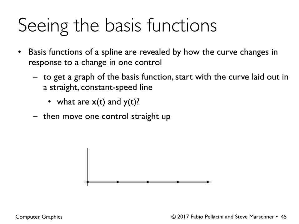
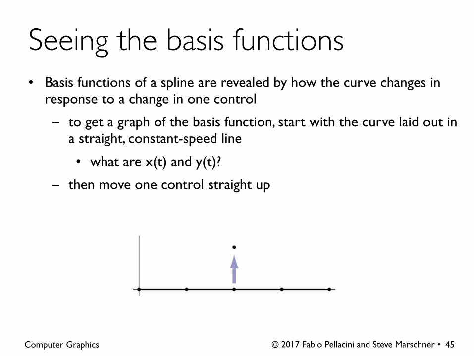
• Basis functions of a spline are revealed by how the curve changes in response to a change in one control
– to get a graph of the basis function, start with the curve laid out in a straight, constant-speed line
• what are x(t) and y(t)?
– then move one control straight up
© 2017 Fabio Pellacini and Steve Marschner • Computer Graphics
Seeing the basis functions
45
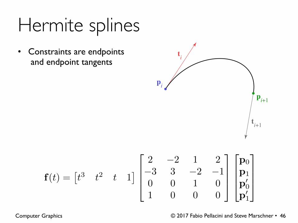
• Constraints are endpoints and endpoint tangents
© 2017 Fabio Pellacini and Steve Marschner • Computer Graphics
Hermite splines
46
f(t) =⇥t3 t2 t 1
⇤
2
664
2 �2 1 2�3 3 �2 �10 0 1 01 0 0 0
3
775
2
664
p0
p1
p00
p01
3
775
ti
pi+1
pi
ti+1
© 2017 Fabio Pellacini and Steve Marschner • Computer Graphics
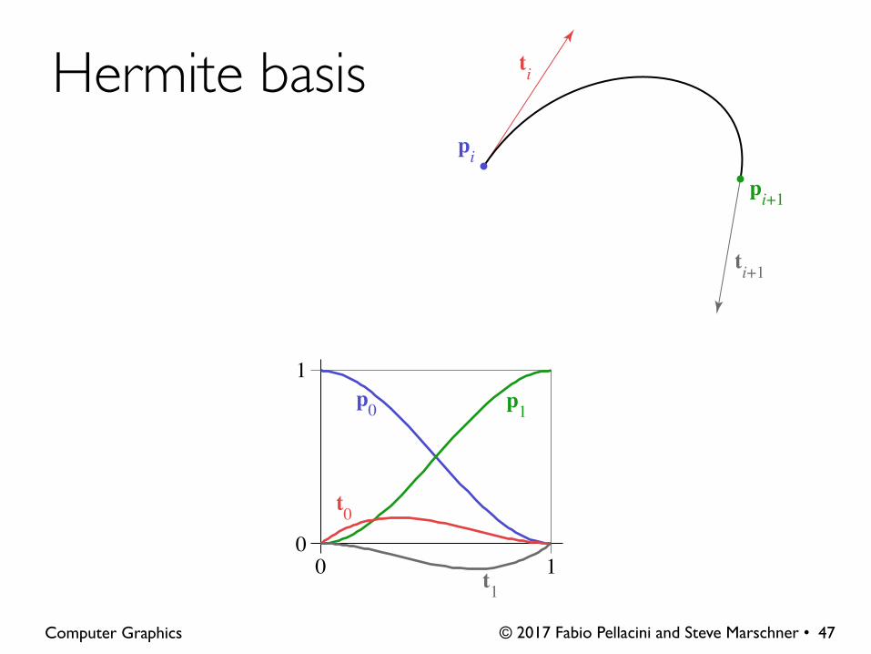
Hermite basis
47
© 2017 Fabio Pellacini and Steve Marschner • Computer Graphics
Hermite basis
47
00 1
1p1
t0
p0
t1
ti
pi+1
pi
ti+1
© 2017 Fabio Pellacini and Steve Marschner • Computer Graphics
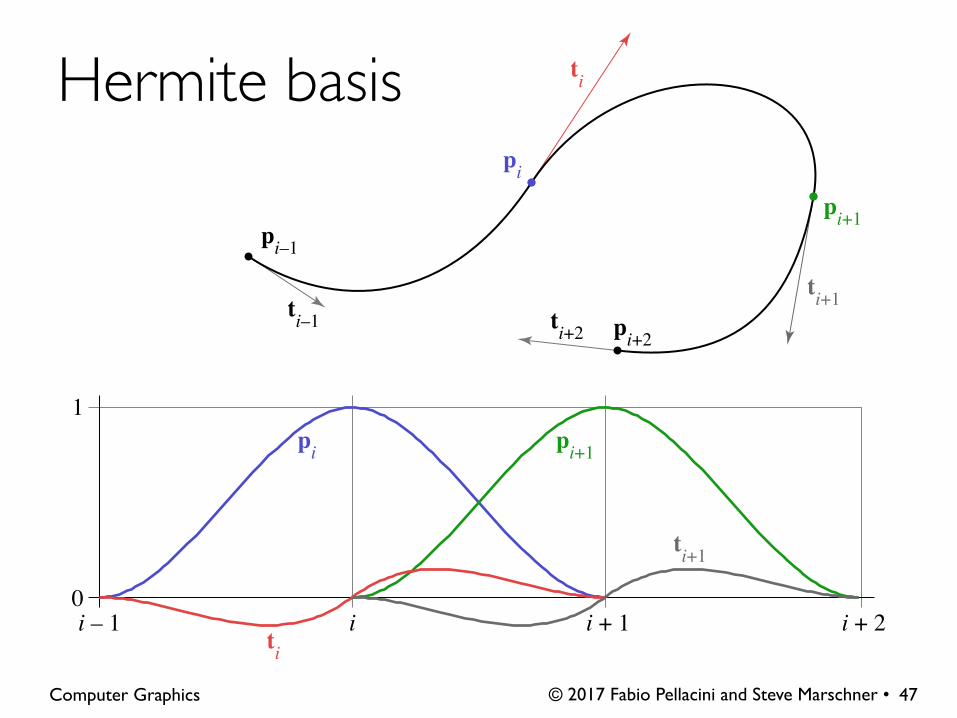
Hermite basis
47
0
1
i i + 1i – 1 i + 2
pi+1
ti
pi
ti+1
ti
pi+1
pi
ti+1
pi–1
ti–1 ti+2 pi+2

© 2017 Fabio Pellacini and Steve Marschner • Computer Graphics
Bézier basis
48
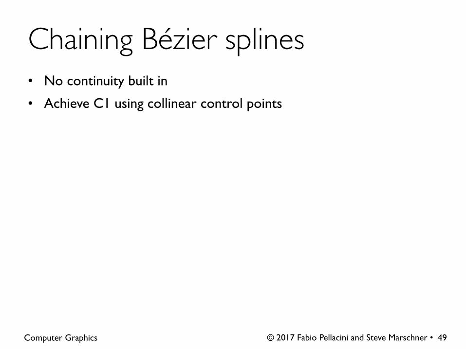
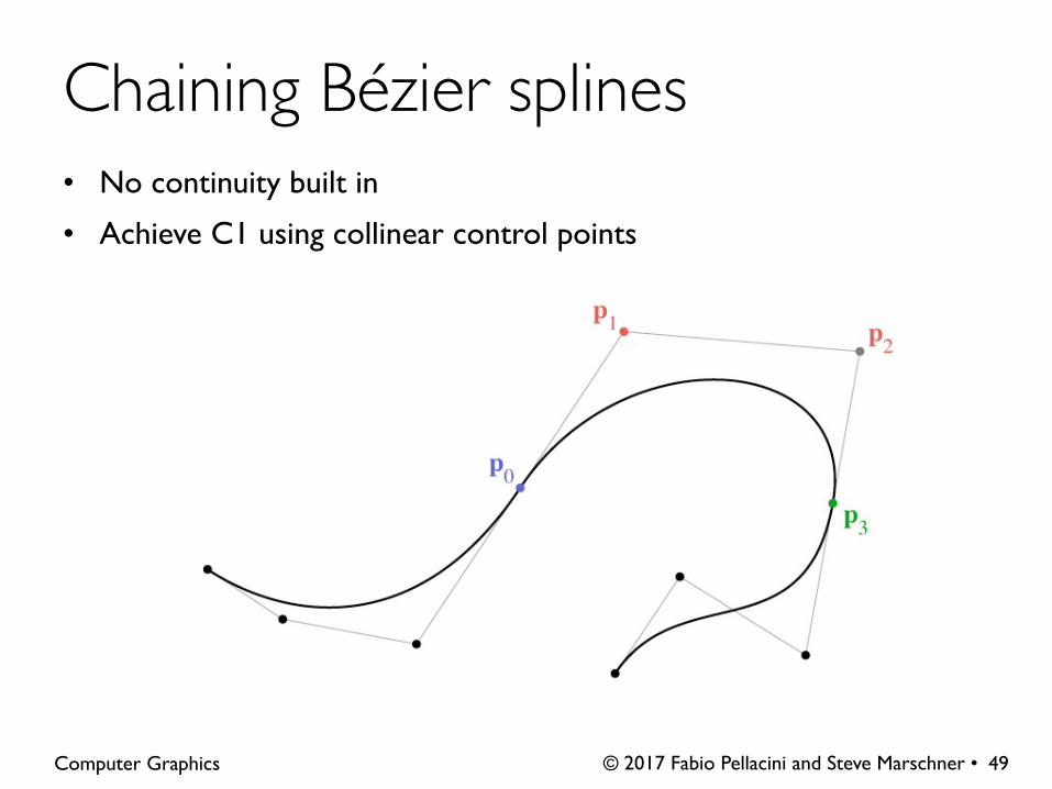
• No continuity built in
• Achieve C1 using collinear control points
© 2017 Fabio Pellacini and Steve Marschner • Computer Graphics
Chaining Bézier splines
49
• No continuity built in
• Achieve C1 using collinear control points
© 2017 Fabio Pellacini and Steve Marschner • Computer Graphics
Chaining Bézier splines
49

• Smoothness can be described by degree of continuity
– zero-order (C0): position matches from both sides
– first-order (C1): tangent matches from both sides
– second-order (C2): curvature matches from both sides
– Gn vs. Cn
© 2017 Fabio Pellacini and Steve Marschner • Computer Graphics
zero order first order second order
Continuity
50
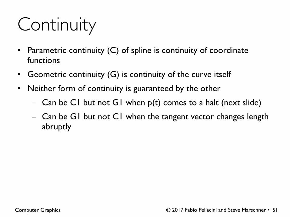
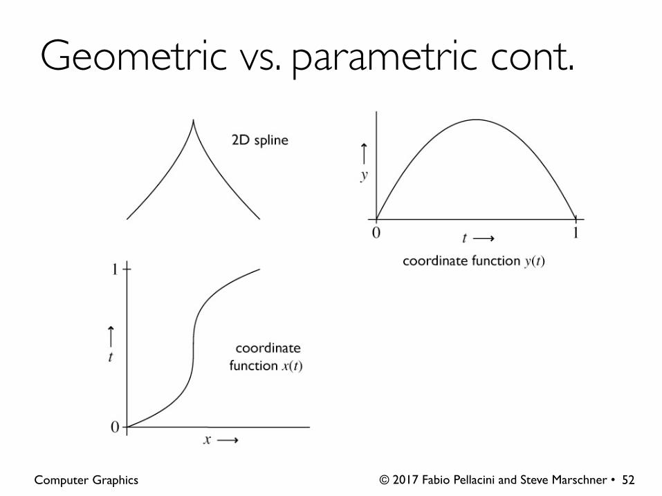
• Parametric continuity (C) of spline is continuity of coordinate functions
• Geometric continuity (G) is continuity of the curve itself
• Neither form of continuity is guaranteed by the other
– Can be C1 but not G1 when p(t) comes to a halt (next slide)
– Can be G1 but not C1 when the tangent vector changes length abruptly
© 2017 Fabio Pellacini and Steve Marschner • Computer Graphics
Continuity
51

© 2017 Fabio Pellacini and Steve Marschner • Computer Graphics
Geometric vs. parametric cont.
52
© 2017 Fabio Pellacini and Steve Marschner • Computer Graphics
Geometric vs. parametric cont.
52

© 2017 Fabio Pellacini and Steve Marschner • Computer Graphics
Geometric vs. parametric cont.
52

• Hermite curves are convenient because they can be made long easily
• Bézier curves are convenient because their controls are all points
– but it is fussy to maintain continuity constraints
– and they interpolate every 3rd point, which is a little odd
• We derived Bézier from Hermite by defining tangents from control points
– a similar construction leads to the interpolating Catmull-Rom spline
© 2017 Fabio Pellacini and Steve Marschner • Computer Graphics
Chaining spline segments
53
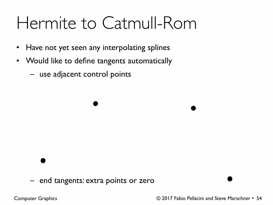
• Have not yet seen any interpolating splines
• Would like to define tangents automatically
– use adjacent control points
– end tangents: extra points or zero
© 2017 Fabio Pellacini and Steve Marschner • Computer Graphics
Hermite to Catmull-Rom
54

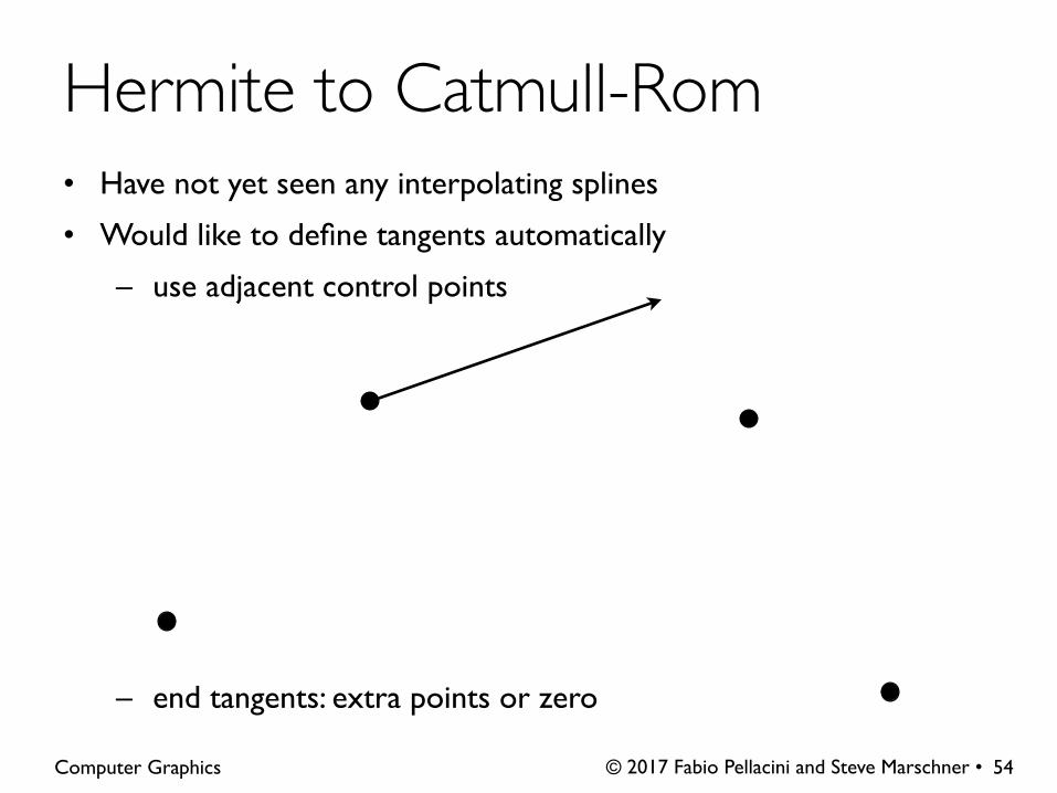
• Have not yet seen any interpolating splines
• Would like to define tangents automatically
– use adjacent control points
– end tangents: extra points or zero
© 2017 Fabio Pellacini and Steve Marschner • Computer Graphics
Hermite to Catmull-Rom
54
• Have not yet seen any interpolating splines
• Would like to define tangents automatically
– use adjacent control points
– end tangents: extra points or zero
© 2017 Fabio Pellacini and Steve Marschner • Computer Graphics
Hermite to Catmull-Rom
54

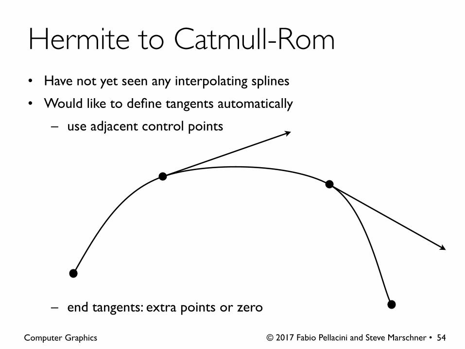
• Have not yet seen any interpolating splines
• Would like to define tangents automatically
– use adjacent control points
– end tangents: extra points or zero
© 2017 Fabio Pellacini and Steve Marschner • Computer Graphics
Hermite to Catmull-Rom
54

• Have not yet seen any interpolating splines
• Would like to define tangents automatically
– use adjacent control points
– end tangents: extra points or zero
© 2017 Fabio Pellacini and Steve Marschner • Computer Graphics
Hermite to Catmull-Rom
54
• Have not yet seen any interpolating splines
• Would like to define tangents automatically
– use adjacent control points
– end tangents: extra points or zero
© 2017 Fabio Pellacini and Steve Marschner • Computer Graphics
Hermite to Catmull-Rom
54
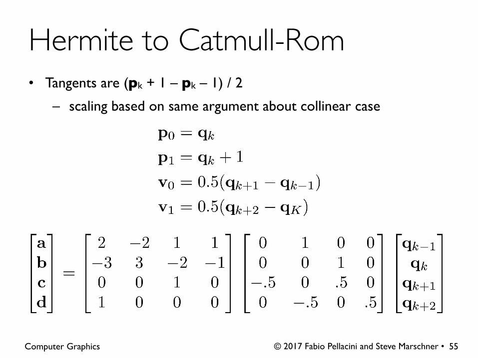
• Tangents are (pk + 1 – pk – 1) / 2
– scaling based on same argument about collinear case
© 2017 Fabio Pellacini and Steve Marschner • Computer Graphics
Hermite to Catmull-Rom
55

© 2017 Fabio Pellacini and Steve Marschner • Computer Graphics
Catmull-Rom basis
56

© 2017 Fabio Pellacini and Steve Marschner • Computer Graphics
Catmull-Rom basis
56
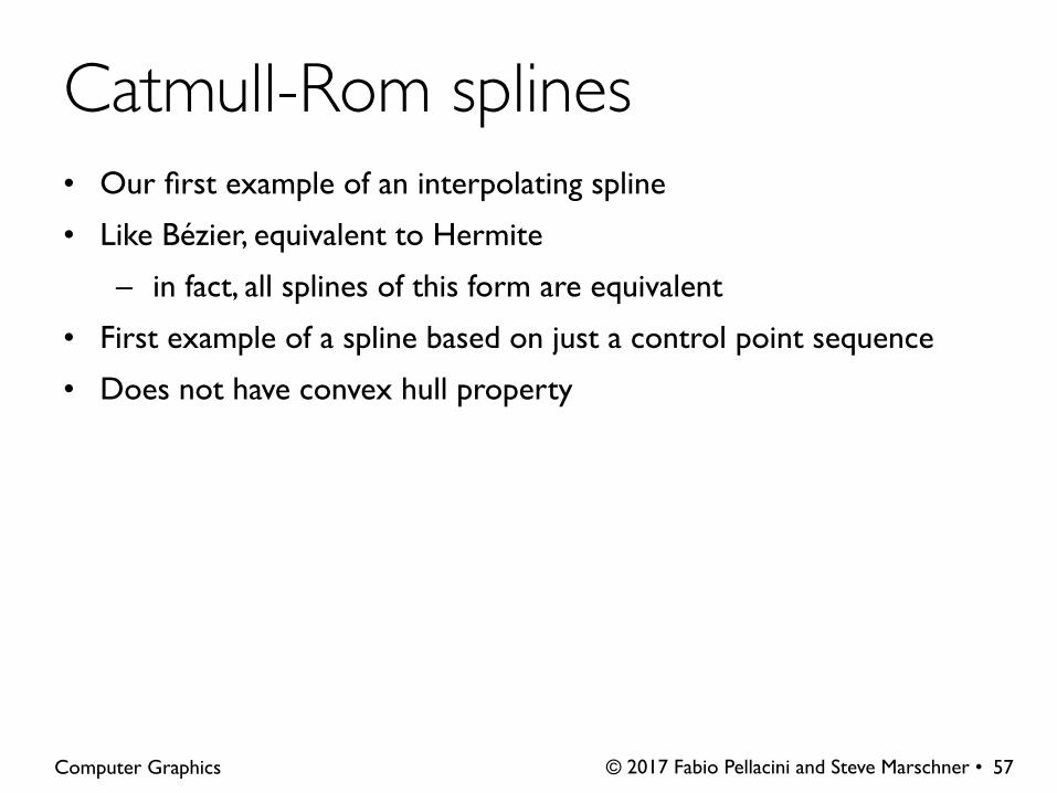
• Our first example of an interpolating spline
• Like Bézier, equivalent to Hermite
– in fact, all splines of this form are equivalent
• First example of a spline based on just a control point sequence
• Does not have convex hull property
© 2017 Fabio Pellacini and Steve Marschner • Computer Graphics
Catmull-Rom splines
57
• We may want more continuity than C1
• We may not need an interpolating spline
• B-splines are a clean, flexible way of making long splines with arbitrary order of continuity
• Various ways to think of construction
– a simple one is convolution
– relationship to sampling and reconstruction
© 2017 Fabio Pellacini and Steve Marschner • Computer Graphics
B-splines
58
© 2017 Fabio Pellacini and Steve Marschner • Computer Graphics
Cubic B-spline basis
59
© 2017 Fabio Pellacini and Steve Marschner • Computer Graphics
Cubic B-spline basis
59
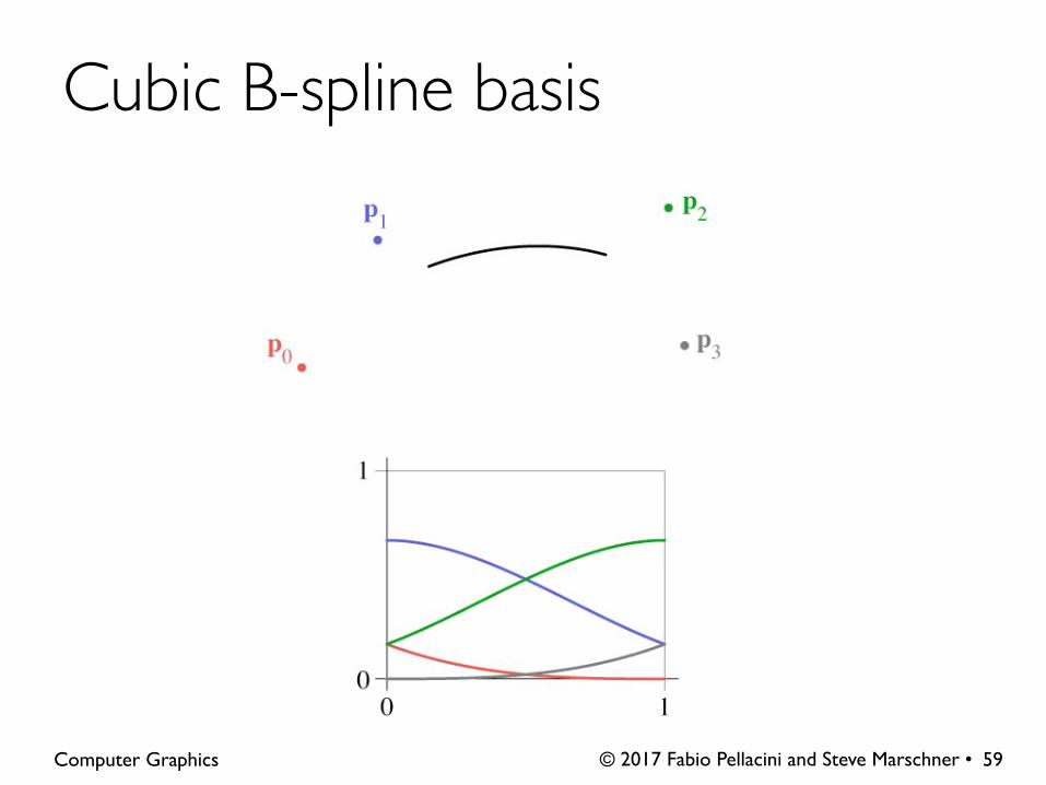
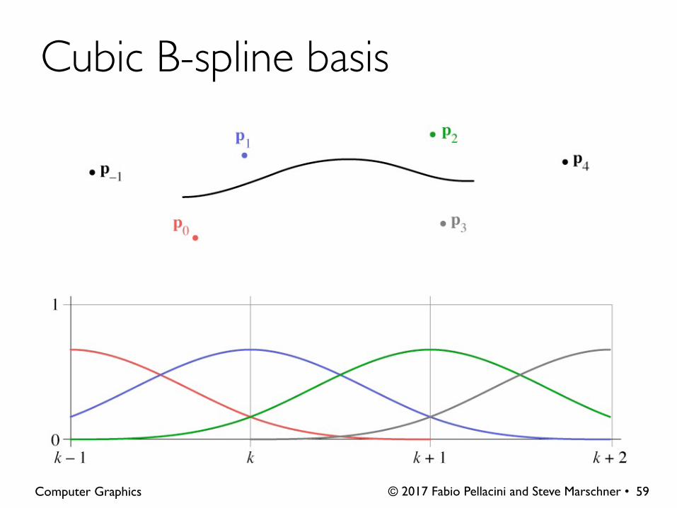
• Approached from a different tack than Hermite-style constraints
– Want a cubic spline; therefore 4 active control points
– Want C2 continuity
– Turns out that is enough to determine everything
© 2017 Fabio Pellacini and Steve Marschner • Computer Graphics
Deriving the B-Spline
60
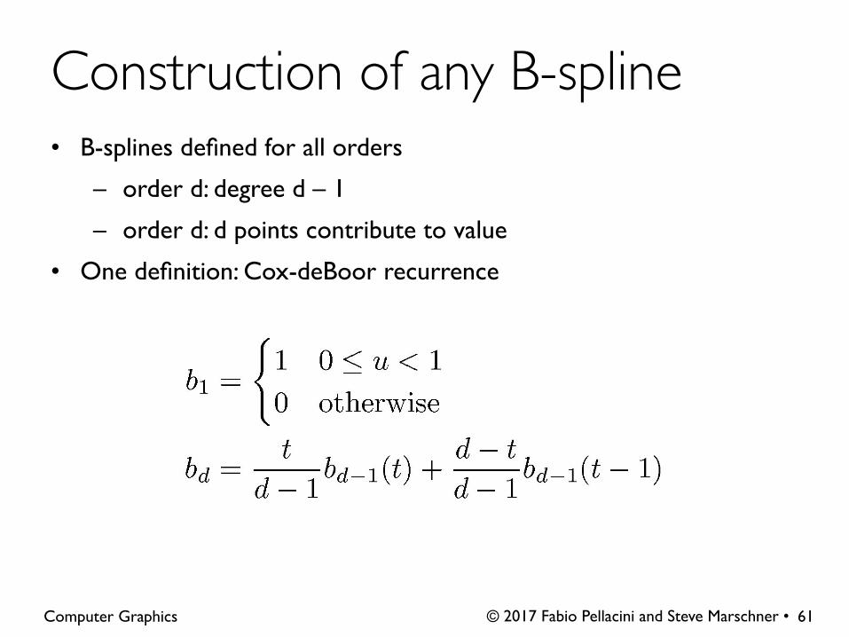
• B-splines defined for all orders
– order d: degree d – 1
– order d: d points contribute to value
• One definition: Cox-deBoor recurrence
© 2017 Fabio Pellacini and Steve Marschner • Computer Graphics
Construction of any B-spline
61
© 2017 Fabio Pellacini and Steve Marschner • Computer Graphics
Cubic B-spline matrix
62
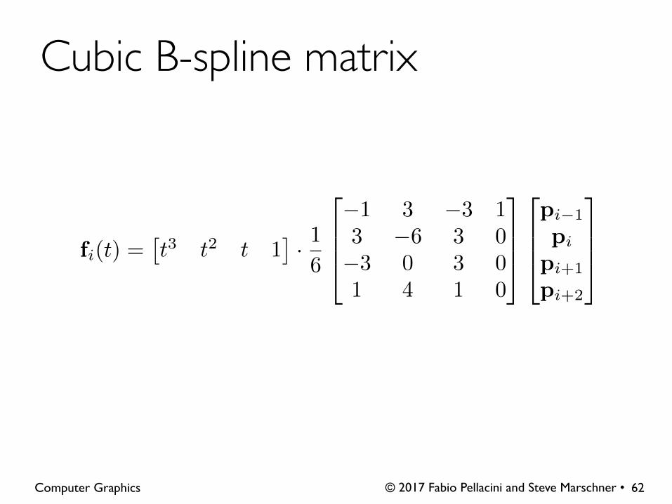
fi(t) =⇥t3 t2 t 1
⇤· 16
2
664
�1 3 �3 13 �6 3 0�3 0 3 01 4 1 0
3
775
2
664
pi�1
pi
pi+1
pi+2
3
775

© 2017 Fabio Pellacini and Steve Marschner • Computer Graphics
Cubic B-spline basis
63

© 2017 Fabio Pellacini and Steve Marschner • Computer Graphics
Cubic B-spline basis
63
• Nonuniform B-splines
– discontinuities not evenly spaced
– allows control over continuity or interpolation at certain points
– e.g. interpolate endpoints (commonly used case)
• Nonuniform Rational B-splines (NURBS)
– ratios of nonuniform B-splines: x(t) / w(t); y(t) / w(t)
– key properties:
• invariance under perspective as well as affine
• ability to represent conic sections exactly
© 2017 Fabio Pellacini and Steve Marschner • Computer Graphics
Other types of B-splines
64

© 2017 Fabio Pellacini and Steve Marschner • Computer Graphics
Refinement and Evaluation
65
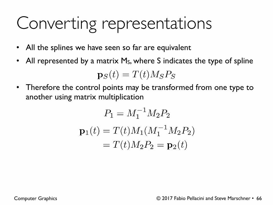
• All the splines we have seen so far are equivalent
• All represented by a matrix MS, where S indicates the type of spline
• Therefore the control points may be transformed from one type to another using matrix multiplication
© 2017 Fabio Pellacini and Steve Marschner • Computer Graphics
Converting representations
66
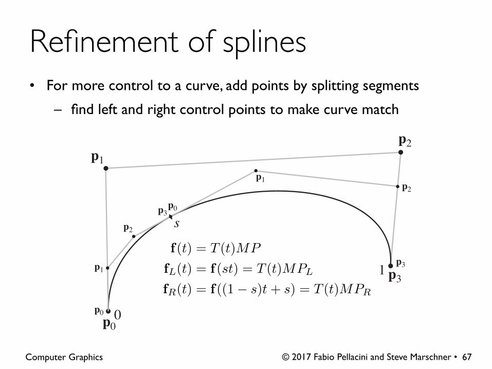
• For more control to a curve, add points by splitting segments
– find left and right control points to make curve match
© 2017 Fabio Pellacini and Steve Marschner • Computer Graphics
Refinement of splines
67
s
0p0
p1
p2
p3
p3
p0
p1p2
p0
p1p2
p31f(t) = T (t)MP
fL(t) = f(st) = T (t)MPL
fR(t) = f((1� s)t+ s) = T (t)MPR

© 2017 Fabio Pellacini and Steve Marschner • Computer Graphics
Refinement math
68
SL =
2
664
s3
s2
s1
3
775
SR =
2
664
s3
3s2(1� s) s2
3s(1� s)2 2s(1� s) s(1� s)3 (1� s)2 (1� s) 1
3
775
fL(t) = T (st)MP = T (t)SLMP
= T (t)M(M�1SLMP )
= T (t)MPL
PL = M�1SLMP
PR = M�1SRMP

• For cubic Bézier, refinement can also be derived from geometric interpretation
© 2017 Fabio Pellacini and Steve Marschner • Computer Graphics
Refinement of Bézier splines
69
[FvD
FH]
qi(↵) = ↵pi + (1� ↵)pi+1
ri(↵) = ↵qi(↵) + (1� ↵)qi+1(↵)
p(↵) = ↵pi(↵) + (1� ↵)pi+1(↵)
fL(↵) defined by {p0,q0(↵), r0(↵),p(↵)}fR(↵) defined by {p(↵), r1(↵),q2(↵),p3}
• Need to generate a list of line segments to draw
– generate efficiently
– use as few as possible
– guarantee approximation accuracy
• Approaches
– recursive subdivision (easy to do adaptively)
– uniform sampling (easy to do efficiently)
© 2017 Fabio Pellacini and Steve Marschner • Computer Graphics
Tesselating splines for display
70
• Recursively split spline using refinement algorithm
– stop when polygon is within epsilon of curve
• Termination criteria
– distance between control points
– distance of control points from line
– angles in control polygon
• Pros: efficient in the number of generated segments
• Cons: inefficient in computation since it requires recursive evaluation
© 2017 Fabio Pellacini and Steve Marschner • Computer Graphics
Tesselation by subdivision
71
• Pick a priori a number of line segments n
• Evaluate the curve at fixed values in t = 1/n
• Pros: very efficient evaluation
• Cons: no guarantees on accuracy and likely to generate too many segments
© 2017 Fabio Pellacini and Steve Marschner • Computer Graphics
Tesselation by sampling
72


![TWISTED SPIN CURVES - uniroma1.it · integral curves, by Altman and Kleiman [AK], and geometrically connected, possibly reducible, nodal curves, by Oda and Seshadri [OS]. A common](https://img.pdfslide.us/doc/110x75/5f652245985c4b182a17192f/twisted-spin-curves-integral-curves-by-altman-and-kleiman-ak-and-geometrically.jpg)


![Multi-objective optimum stator and rotor stagger angle ...scientiairanica.sharif.edu/article_3658_4b9c5ea15d4859b...Researchers Curves Applications Oyama et al. [4] B-spline curves](https://img.pdfslide.us/doc/110x75/6058611f8e9ea109717b1459/multi-objective-optimum-stator-and-rotor-stagger-angle-researchers-curves.jpg)