Hermite and spline interpolation algorithms forplanar & spatial Pythagorean-hodograph curves

Rida T. Farouki

Department of Mechanical & Aeronautical Engineering,University of California, Davis

— synopsis —

• motivation for Hermite & spline interpolation algorithms

• planar PH quintic Hermite interpolants (four solutions)

• computing absolute rotation index & elastic bending energy

• a priori identification of “good” Hermite interpolant

• planar C2 PH quintic splines — numerical methods

• spatial PH quintic Hermite interpolants (2 free parameters)

• spatial PH quintics — taxonomy of special types

• spatial C2 PH quintic splines — residual freedoms

motivation for Hermite & spline interpolation algorithms

• only cubic PH curves characterizable by simple constraintson Bezier control polygons

• planar PH cubics = Tschirnhausen’s cubic,spatial PH cubics = {helical cubic space curves }— too limited for general free–form design applications

• construct quintic PH curves “geometrically” by interpolationof discrete data — points, tangents, etc.

• non–linear interpolation equations made tractable bycomplex number model for planar PH curves, andquaternion or Hopf map model for spatial PH curves

• efficient algorithms allow interactive design of PH curves

Pythagorean triples of polynomials

x′2(t) + y′2(t) = σ2(t) ⇐⇒

x′(t) = u2(t)− v2(t)y′(t) = 2 u(t)v(t)σ(t) = u2(t) + v2(t)

K. K. Kubota, Pythagorean triples in unique factorization domains, American Mathematical Monthly79, 503–505 (1972)

R. T. Farouki and T. Sakkalis, Pythagorean hodographs, IBM Journal of Research and Development34 736–752 (1990)

R. T. Farouki, The conformal map z → z2 of the hodograph plane, Computer Aided Geometric Design11, 363–390 (1994)

complex number model for planar PH curves

choose complex polynomial w(t) = u(t) + i v(t)

→ planar Pythagorean hodograph r′(t) = (x′(t), y′(t)) = w2(t)

planar PH quintic Hermite interpolants

R. T. Farouki and C. A. Neff, Hermite interpolation by Pythagorean–hodograph quintics,Mathematics of Computation 64, 1589–1609 (1995)

complex representation: hodograph = [ complex quadratic polynomial ] 2

r′(t) = [w0(1− t)2 + w12(1− t)t + w2t2 ] 2

r(t) =∫

r′(t) dt =5∑

k=0

pk

(5k

)(1− t)5−ktk

complex Hermite data — r′(0) = d0, r′(1) = d1, r(1)− r(0) = ∆p

→ three quadratic equations in three complex variables w0, w1, w2

w20 = d0 , w2

2 = d1 , w20 + w0w1 +

2w21 + w2w0

3+ w1w2 + w2

2 = 5∆p

generically four distinct interpolants to given Hermite data d0, d1, ∆p

one good solution among four PH quintic interpolants —other three typically exhibit undesired “looping” behavior

obtain Bezier control points of PH quintic from w0, w1, w2

p1 = p0 +w2

0

5,

p2 = p1 +w0w1

5,

p3 = p2 +2w2

1 + w0w2

15,

p4 = p3 +w1w2

5,

p5 = p4 +w2

2

5.

four distinct PH quintic Hermite interpolants

+ + + –

– + – –

blue = PH quintic, red = “ordinary” cubic

choosing the “good” interpolant — rotation index

absolute rotation index: Rabs =12π

∫|κ| ds

w.l.o.g. take r(0) = 0 and r(1) = 1 (shift + scale of Hermite data)

r′(t) = k [ (t− a)(t− b) ]2

solve for k, a, b instead of w0, w1, w2

locations of a, b relative to [ 0, 1 ] gives Rabs :

Rabs =∠ 0a 1 + ∠ 0b 1

π(no inflections)

Rabs =1π

N∑k=0

|∠ tk a tk+1 − ∠ tk b tk+1 |

Computation of absolute rotation index Rabs from locations of the complexhodograph roots a, b relative to t ∈ [ 0, 1 ]. The best interpolant ariseswhen a, b lie on opposite sides of (and are not close to) this interval.

choosing the “good” interpolant — bending energy

U =∫

κ2 ds =∫|r′ × r′′|2

σ5dt

use complex form r′(t) = w2(t) with w(t) = k(t− a)(t− b) again

analytic reduction of indefinite integral

U(t) =4|k|2

{2 Re(a1) ln |t− a| + 2Re(b1) ln |t− b|

− 2 Im(a1) arg(t− a) − 2 Im(b1) arg(t− b)

− Re[

2a2

t− a+

2b2

t− b+

a3

(t− a)2+

b3

(t− b)2

] }.

a1,b1,a2,b2,a3,b3 = coefficients in partial fraction expansion of integrand

total bending energy of PH quintic E = U(1)− U(0)

compare PH quintic & “ordinary” cubic interpolants

good PH quintic interpolants (blue) to first-order Hermite data typicallyhave lower bending energy than “ordinary” cubic interpolants (red)

C2 spatial Hermite interpolants:

B. Juttler, C2 Hermite interpolation by Pythagorean hodograph curves of degree seven,Mathematics of Computation 70, 1089–1111 (2001)

monotone–curvature PH quintic segments

D. J. Walton and D. S. Meek, A Pythagorean–hodograph quintic spiral, Computer Aided Design28, 943–950 (1996)

R. T. Farouki, Pythagorean–hodograph quintic transition curves of monotone curvature,Computer Aided Design 29, 601–606 (1997)

k = 3.50 k = 3.75 k = 4.00

G2 blends between a line and a circle, defined by PH quintics of monotonecurvature (the Bezier control polygons of the PH quintics are also shown)— the free parameter k controls the rate of increase of the curvature.

a priori identification of “good” interpolant

H. P. Moon, R. T. Farouki, and H. I. Choi, Construction and shape analysis of PH quintic Hermiteinterpolants, Computer Aided Geometric Design 18, 93–115 (2001)

H. I. Choi, R. T. Farouki, S. H. Kwon, and H. P. Moon, Topological criterion for selection of quinticPythagorean–hodograph Hermite interpolants, Computer Aided Geometric Design 25, 411–433 (2008)

if the end derivatives d0, d1 lie in complex–plane domain D defined by

D = {d | Re(d) > 0 and |d| < 3 }

— i.e., they point in the direction of ∆p and have magnitudescommensurate with |∆p|, the “good” PH quintic corresponds to

the ++ choice of signs in the solution procedure

criterion for “good” solution — absence of anti–parallel tangentsrelative to the “ordinary” cubic Hermite interpolant

construction of C2 PH quintic splinesversus “ordinary” C2 cubic splines

• both incur global system of equations in three consecutive unknowns

• both require specification of end conditions to complete the equations

• equations for “ordinary” cubic splines arise from C2 continuity conditionat each interior node, while equations for PH quintic splines arise frominterpolating consecutive points pi, pi+1

• “ordinary” cubic splines incur linear equations in real variables, butPH quintic splines incur quadratic equations in complex variables

• coordinate components of “ordinary” cubic splines weakly coupledthrough nodal parameter values; components of PH quintic splinesstrongly coupled through PH property

• linearity of “ordinary” cubic splines ⇒ unique interpolant andspline basis methods, but non–linear nature of PH quintic splines⇒ multiplicity of solutions and no linear superposition

planar C2 PH quintic spline equations

problem: construct C2 piecewise–PH–quintic curve interpolating givensequence of points p0, . . . ,pN ∈ R2

using complex representation of planar PH quintics, write hodograph ofsegment ri(t) between pi−1 and pi, as square of a complex quadratic:

r′i(t) = [ 12(zi−1 + zi)(1− t)2 + zi 2(1− t)t + 1

2(zi + zi+1)t2 ]2

⇒ ri(t) and ri+1(t) automatically satisfy C1 and C2 conditions at theirjuncture pi = ri(1) = ri+1(0) — namely,

r′i(1) = r′i+1(0) = 14(zi + zi+1)2, r′′i (1) = r′′i+1(0) = (zi+1 − zi)(zi + zi+1)

writing ∆pi = pi − pi−1, the end–point interpolation condition∫ 1

0

r′i(t) dt = ∆pi

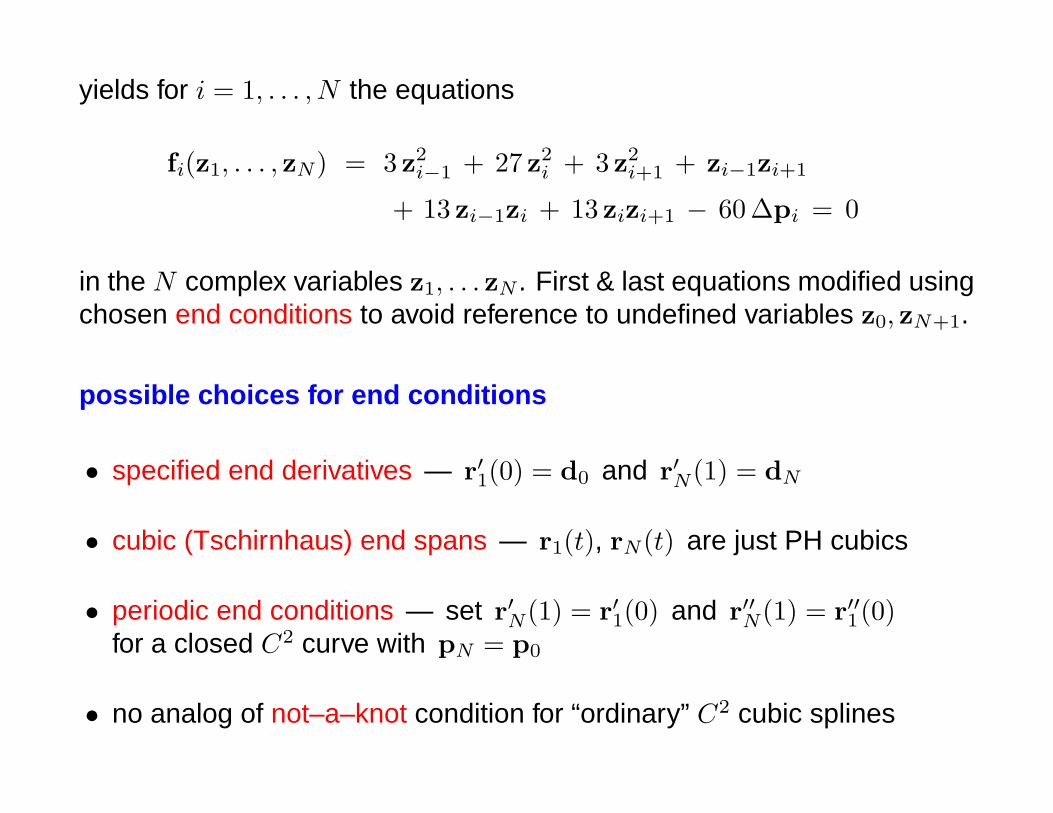
yields for i = 1, . . . , N the equations

fi(z1, . . . , zN) = 3 z2i−1 + 27 z2

i + 3 z2i+1 + zi−1zi+1

+ 13 zi−1zi + 13 zizi+1 − 60 ∆pi = 0

in the N complex variables z1, . . . zN . First & last equations modified usingchosen end conditions to avoid reference to undefined variables z0, zN+1.

possible choices for end conditions

• specified end derivatives — r′1(0) = d0 and r′N(1) = dN

• cubic (Tschirnhaus) end spans — r1(t), rN(t) are just PH cubics

• periodic end conditions — set r′N(1) = r′1(0) and r′′N(1) = r′′1(0)for a closed C2 curve with pN = p0

• no analog of not–a–knot condition for “ordinary” C2 cubic splines

solution method #1 — homotopy scheme

G. Albrecht and R. T. Farouki, Construction of C2 Pythagorean–hodograph interpolating splines bythe homotopy method , Advances in Computational Mathematics 5, 417–442 (1996)

the non–linear system to be solved: fi(z1, . . . , zN) = 0 , 1 ≤ i ≤ N

“initial” system with known solutions: gi(z1, . . . , zN) = 0 , 1 ≤ i ≤ N

“continuously deform” initial system into desired system whiletracking all solutions as homotopy parameter λ increases from 0 to 1

hi(z1, . . . , zN , λ) = λ fi(z1, . . . , zN) + (1− λ) eiφ gi(z1, . . . , zN) = 0

2N+k non-singular solution loci (z1, . . . , zN , λ) ∈ CN × R for “almost all” φ

predictor-corrector method

trace from λ = 0 to 1 loci defined by hi(z1, . . . , zN , λ) = 0, 1 ≤ i ≤ N

tridiagonal Jacobian matrix: Mij =∂hi

∂zj, 1 ≤ i, j ≤ N

predictor step : motion along tangent directions to solution lociN∑

j=1

Mij ∆zj = (eiφ gi − fi) ∆λ , i = 1, . . . , N

corrector step : correct for curvature of loci by Newton iterations

z(r+1)j = z(r)

j + δzj for j = 1, . . . , N , r = 1, 2, . . .

whereN∑

j=1

M(r)ij δzj = − h(r)

i , i = 1, . . . , N

untilN∑

i=1

|hi(z(r)1 , . . . , z(r)

N , λ + ∆λ) |2 ≤ ε2

0.0 0.2 0.4 0.6 0.8 1.00

200

400

600

λ

0

100

200

300

400

500

600

700

typical behavior of ‖f‖2, ‖g‖2, ‖h‖2 norms in predictor–corrector scheme

• well–conditioned — accuracy near machine precision achievable

• gives complete set of 2N+k distinct PH quintic spline interpolants(k = −1, 0,+1 depends on chosen end conditions)

• unique good interpolant — without undesired “looping” behavior

• better shape (curvature distribution) than “ordinary” C2 cubic spline

• becomes computationally very expensive for large N

complete set of PH quintic spline interpolants

shape measures for identifying “good” interpolant:

total arc length, absolute rotation index, elastic bending energy

S =∫

ds , Rabs =12π

∫|κ| ds , E =

∫κ2 ds

comparison of PH quintic & “ordinary” cubic splines

0 1 2 3 4 5 6 7 8 9–4

0

4

8

12

16

20

t

κ

blue = C2 PH quintic spline, red = “ordinary” C2 cubic spline

solution method #2 — Newton-Raphson iteration

R. T. Farouki, B. K. Kuspa, C. Manni, and A. Sestini, Efficient solution of the complex quadratictridiagonal system for C2 PH quintic splines, Numerical Algorithms 27, 35–60 (2001)

in applications, we want to compute only the “good” PH quintic spline

apply Newton-Raphson iteration to system fi(z1, . . . , zN) = 0 , 1 ≤ i ≤ N

recall that Jacobian matrix Mij =∂ fi∂ zj

, 1 ≤ i, j ≤ N is tridiagonal

in rows i = 2, . . . , N − 1, the only non–zero elements are

Mi,i−1 = 6 zi−1 + 13 zi + zi+1 ,

Mii = 13 zi−1 + 54 zi + 13 zi+1 ,

Mi,i+1 = zi−1 + 13 zi + 6 zi+1 .

rows i = 1 and i = N are modified to reflect the chosen end conditions

writing z = (z1, . . . , zN)T and f = (f1, . . . , fN)T , the Newton–Raphsoniterations may be expressed as

z(r+1) = z(r) + δz(r) , r = 0, 1, 2, . . .

where δz(r) = (δz(r)1 , . . . , δz(r)

N )T is the solution of the linear system

M(r) δz(r) = − f (r) .

superscripts on M and f indicate evaluation at z(r) = (z(r)0 , . . . , z(r)

N ).

key step: find “sufficiently close” initial approximation z(0) = (z(0)1 , . . . , z(0)

N )

Kantorovich theorem: guaranteed convergence under verifiable conditions

choice of starting approximation

critical to successful Kanotorovich test & rapid convergence of iterations

strategy: equate mid–point derivatives of PH quintic spline to (known)mid–point derivatives of “ordinary” cubic spline that interpolates the samedata points p0, . . . ,pN

yields a tridiagonal linear system for starting values z1, . . . , zN

zi−1 + 6zi + zi+1 = 4√

6∆pi − (di−1 + di) , i = 1, . . . , N

where d0, . . . ,dN are the nodal derivatives of the “ordinary” cubic spline,and equations i = 1 and i = N are adjusted for the chosen end conditions

strategy is nearly infallible for smoothly–varying data points p0, . . . ,pN

efficiency of Newton-Raphson method

tridiagonal equations for NR increments δz(r) — O(N) solution cost —and quadratic convergence of the NR iterations =⇒ extremely efficientconstruction of large–N PH quintic splines

shape N + 1 homotopy method Newton–Raphsonkidney 10 8.09 sec 0.11 secsquiggly 15 656.21 sec 0.12 secquirky 19 1128.97 sec 0.23 secbig open 35 0.40 secbig closed 38 0.43 sec

Timing comparisons for C2 PH quintic spline test curves

big_open big_closed

C2 PH quintic splines computed by Newton–Raphson method for large N

design of C2 PH splines by control polygons

F. Pelosi, M. L. Sampoli, R. T. Farouki, and C. Manni, A control polygon scheme for design of planarC2 PH quintic spline curves, Computer Aided Geometric Design 24, 28–52 (2007)

desire a control–polygon approach to constructing PH splines, thatmimics the familiar and useful properties of cubic B–spline curves

non–linear nature of PH curves =⇒ there is no spline basis for them

strategy: control polygon defines a “hidden” interpolation problem forPH splines, to be solved by efficient Newton–Raphson method

C2 PH quintic spline curve associated with a given control polygon andknot sequence is defined to be the “good” interpolant to the nodal pointsof the ordinary C2 cubic spline curve with the same B–spline controlpoints, knot sequence, and end conditions

comparison of the “ordinary” cubic B–spline (red) and PH quintic spline(blue) curves defined by given control polygons and knot sequences

computation sufficiently fast for interactive modification of polygons

multiple knots may be introduced to reduce the continuity to C1 or C0

linear precision & local modification capability possible with double knots

. . . the three Russian brothers . . .

. . . Following the collapse of the former Soviet Union, theeconomy in Russia hit hard times, and jobs were difficult tofind. Dmitry, Ivan, and Alexey — the Brothers Karamazov —therefore decided to seek their fortunes by emigrating toAmerica, England, Australia . . .

Pythagorean quartuples of polynomials

x′2(t) + y′2(t) + z′2(t) = σ2(t) ⇐⇒

x′(t) = u2(t) + v2(t)− p2(t)− q2(t)y′(t) = 2 [u(t)q(t) + v(t)p(t) ]z′(t) = 2 [ v(t)q(t)− u(t)p(t) ]σ(t) = u2(t) + v2(t) + p2(t) + q2(t)

R. Dietz, J. Hoschek, and B. Juttler, An algebraic approach to curves and surfaces on the sphereand on other quadrics, Computer Aided Geometric Design 10, 211–229 (1993)

R. T. Farouki and T. Sakkalis, Pythagorean–hodograph space curves, Advances in ComputationalMathematics, 2 41–66 (1994)

H. I. Choi, D. S. Lee, and H. P. Moon, Clifford algebra, spin representation, and rationalparameterization of curves and surfaces, Advances in Computational Mathematics 17, 5-48 (2002)

quaternion model for spatial PH curves

choose quaternion polynomial A(t) = u(t) + v(t) i + p(t) j + q(t)k

→ spatial Pythagorean hodograph r′(t) = (x′(t), y′(t), z′(t)) = A(t) iA∗(t)

fundamentals of quaternion algebra

quaternions are four-dimensional numbers of the form

A = a + ax i + ay j + az k and B = b + bx i + by j + bz k

that obey the sum and (non-commutative) product rules

A + B = (a + b) + (ax + bx) i + (ay + by) j + (az + bz)k

AB = (ab− axbx − ayby − azbz)

+ (abx + bax + aybz − azby) i

+ (aby + bay + azbx − axbz) j

+ (abz + baz + axby − aybx)k

basis elements 1, i, j, k satisfy i2 = j2 = k2 = i j k = −1

equivalently, i j = − j i = k , j k = −k j = i , k i = − i k = j

scalar-vector form of quaternions

set A = (a,a) and B = (b,b) — a, b and a, b are scalar and vector parts

(a, b and a,b also called the real and imaginary parts of A,B)

A + B = ( a + b , a + b )

AB = ( ab− a · b , ab + ba + a× b)

(historical note: Hamilton’s quaternions preceded, but were eventuallysupplanted by, the 3-dimensional vector analysis of Gibbs and Heaviside)

A∗ = (a,−a) is the conjugate of A

modulus : |A|2 = A∗A = AA∗ = a2 + |a|2

note that |AB | = |A| |B| and (AB)∗ = B∗A∗

unit quaternions & spatial rotations

any unit quaternion has the form U = (cos 12θ, sin

12θ n)

describes a spatial rotation by angle θ about unit vector n

for any vector v the quaternion product

v = U vU∗

yields the vector v corresponding to a rotation of v by θ about n

here v is short-hand for a “pure vector” quaternion V = (0,v)

unit quaternions U form a (non-commutative) group under multiplication

quaternion model for spatial PH curves

quaternion polynomial A(t) = u(t) + v(t) i + p(t) j + q(t)k

maps to r′(t) = A(t) iA∗(t) = [u2(t) + v2(t)− p2(t)− q2(t) ] i

+ 2 [ u(t)q(t) + v(t)p(t) ] j + 2 [ v(t)q(t)− u(t)p(t) ]k

rotation invariance of spatial PH form: rotate by θ about n = (nx, ny, nz)

define U = (cos 12θ, sin

12θ n) — then r′(t) → r′(t) = A(t) i A∗(t)

where A(t) = U A(t) (can interpret as rotation in R4)

solution of “fundamental” quaternion equation

for any given vector v, find quaternions A satisfying A iA∗ = v

such quaternions A map the unit vector i onto the given vector vby means of a scaling–rotation transformation

write v =v|v|

= (λ, µ, ν) — obtain one–parameter family of solutions

A =

√(1 + λ)|v|

2

(− sinφ + cos φ i +

µ cos φ + ν sinφ

1 + λj +

ν cos φ− µ sinφ

1 + λk)

where φ = free angular variable

more compact from — A =√|v|n exp(φ i)

where exp(φ i) = cos φ + sinφ i and n =i + v| i + v |

= bisector of i, v

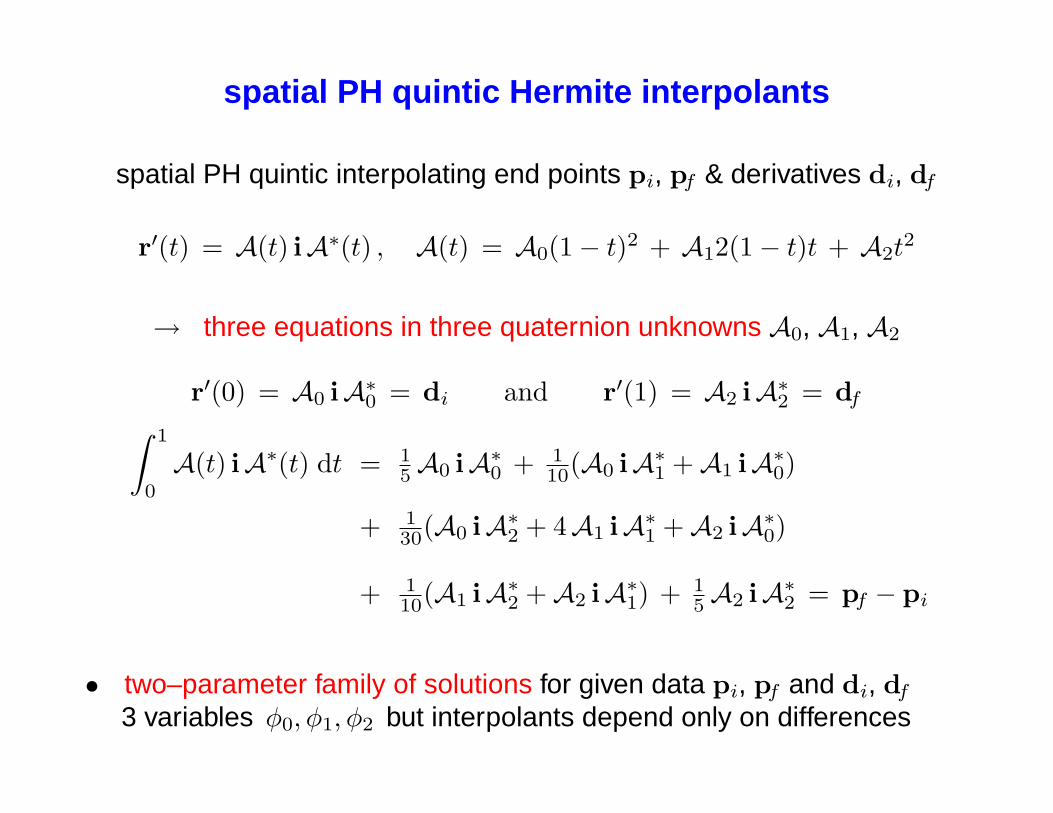
spatial PH quintic Hermite interpolants

spatial PH quintic interpolating end points pi, pf & derivatives di, df

r′(t) = A(t) iA∗(t) , A(t) = A0(1− t)2 + A12(1− t)t + A2t2

→ three equations in three quaternion unknowns A0, A1, A2

r′(0) = A0 iA∗0 = di and r′(1) = A2 iA∗2 = df∫ 1

0

A(t) iA∗(t) dt = 15A0 iA∗0 + 1

10(A0 iA∗1 +A1 iA∗0)

+ 130(A0 iA∗2 + 4A1 iA∗1 +A2 iA∗0)

+ 110(A1 iA∗2 +A2 iA∗1) + 1

5A2 iA∗2 = pf − pi

• two–parameter family of solutions for given data pi, pf and di, df

3 variables φ0, φ1, φ2 but interpolants depend only on differences

examples of spatial PH quintic Hermite interpolants

pi = (0, 0, 0) and pf = (1, 1, 1) for both curves

di = (−0.8, 0.3, 1.2) and df = (0.5,−1.3,−1.0) for curve on left,

di = (0.4,−1.5,−1.2) and df = (−1.2,−0.6,−1.2) for curve on right

choosing free parameters φ0, φ2 (set φ1 = 0 w.l.o.g.)

R. T. Farouki, C. Giannelli, C. Manni, and A. Sestini, Identification of spatial PH quintic Hermiteinterpolants with near–optimal shape measures, Computer Aided Geometric Deisgn 25, 274–297 (2008)

total arc length depends only on difference φ2 − φ0 of two parameters

⇒ one–parameter family of Hermite interpolants with identical arc lengths

the Hermite interpolants of extremal arc length are helical PH curves

minimization of elastic energy E =∫

κ2 ds (computation intensive)

several efficient empirical measures for determining “optimal” φ0, φ2

One–parameter families of spatial PH quintic interpolants, of identical arclength, defined by keeping φ2 − φ0 constant, and varying only 1

2(φ0 + φ2)

taxonomy of “special spatial” PH curves

helical polynomial space curves

curve tangent t makes a constant angle α with a fixed unit vector a— i.e., a · t = cos α (a = axis of helix, α = pitch angle)

equivalently, curve has constant curvature–torsion ratio: κ/τ = tan α

all helical polynomial curves are PH curves (implied by a · t = cos α)

all spatial PH cubics are helical, but not all PH curves of degree ≥ 5

“double” Pythagorean–hodograph (DPH) curves

components of both r′(t) & r′(t)× r′′(t) satisfy Pythagorean conditions

DPH curves have rational Frenet frames (t,n,b) and curvatures κ

all helical polynomial curves must be DPH — not just PH — curves

all DPH quintics are helical, but not all DPH curves of degree ≥ 7

rational rotation–minimizing frame (RRMF) curves

rational adapted frames (t,u,v) with angular velocity satisfying ω · t ≡ 0

RRMF curves are of minimum degree 5 (proper subset of PH quintics)

identifiable by quadratic (vector) constraint on quaternion coefficients

useful in spatial motion planning and rigid–body orientation control

construction through geometric Hermite interpolation algorithm

Frenet

RMF

rational rotation-minimizing rigid body motions

R. T. Farouki, C. Giannelli, C. Manni, A. Sestini (2010), Design of rational rotation–minimizing rigid bodymotions by Hermite interpolation, Math. Comp., submitted

• interpolate end points pi, pf and frames (ti,ui,vi) and (tf ,uf ,vf) byPH quintic r(ξ) with rational rotation-minimizing frame (t(ξ),u(ξ),v(ξ))

• RRMF condition for spatial PH quintics: A1 iA∗1 = A0 iA∗2 +A2 iA∗0

• satisfying RRMF condition & end frame interpolation always possible— end point interpolation requires positive root of degree 6 equation

• diverse applications — to robotics, animation, spatial path planning,geometric sweeping operations, etc.

spatial C2 PH quintic splines

• quaternion and Hopf map models for spatial C2 PH quintic splinecurves interpolating sequence of points p0, . . . ,pN ∈ R3 both incurone residual freedom per spline segment

• shape of spline interpolant sensitive to choice of free parameters

• early study — fix freedoms using “quaternion matching” condition

• optimize shape measure — e.g., proximity to a single PH cubic —to provide control-polygon-based design scheme

• specify arc lengths of spline segments as multiples of chord lengths,∆sk = γk |pk − pk−1| — for γ1 = · · · = γN (= γ, say) we can use γas a single tension parameter to alter interpolant shape

closure

• advantages of PH curves: rational offset curves, analytic real-timeinterpolators, exact bending energy, rotation-minimizing frames, etc.

• complex number and quaternion models are “natural” formulationsfor planar and spatial PH curves — rotation invariance, geometricalinsight, simplified construction algorithms, etc.

• for planar PH curves, efficient & robust Hermite and spline interpolationalgorithms are available for practical use

• for spatial PH curves, basic Hermite interpolation algorithm availablewith methods for “optimal” selection of two free parameters

• open problems for spatial PH curves — choice of multiple freeparameters in C2 spline formulation; geometric Hermite interpolationwith RRMF curves; applications of rotation–minimizing frames inmotion planning, animation, spatial orientation control, etc.