2.852 Lecture 25: An Integrated Quality/Quantity Model of ... · PDF file2.852 Lecture 25: An Integrated Quality/Quantity ... And many practices are used in industries such as statistical

1

2.852 Lecture 25:

An Integrated Quality/Quantity Model of a Transfer Line

Jongyoon Kim Stanley B. Gershwin

Copyright 2003 Jongyoon Kim, Stanley B. Gershwinc

Good afternoon.

Thank you for attending to my presentation.

My name is Jongyoon Kim, a Ph.D. candidate at Massachusetts Institute of Technology.

Today I would like to talk about a issue under the title of “An integrated quality and quantity model of a transfer line” which is funded by PSA Peugeot Citron.

2


AGENDAAGENDA

1. Motivation

2. Research Objectives

3. Research Directions

4. Model Descriptions

5. Preliminary Results

6. Future Research Plan

Agenda.

First I would like to start with motivation of this research.

Then move to research objectives and direction.

I will use most of time to describe my model.

After then, I am going to show some preliminary results.

Finally I will end up with future research plan.

3


MOTIVATIONMOTIVATION

“Effective implementation of quality program leads to significant wealth creation.” (38% to 46% of higher stock value)*

“At 3 sigma level, quality cost accounts for 25 – 40% of Revenue.”**

“A dissatisfied customer will tell 9 to 10 people about an unhappy experience, even if the problem is not serious.”***

*Hendricks and Singhal, Management Science**Harry and et al., “6 Sigma”***Pande, Holpp, “What is 6 Sigma?”

Goal: Perfect Quality!

Quality

A lot of attention is paid to quality in manufacturing industry since 1980s when Japanese manufacturers started to get market shares in U.S.

Various studies have been done to quantify the importance of quality. These are some of them.

According to Consumer Report, Initial quality and reliability of cars are the major determinant of customer decision in U.S.

And that is the reason why American automotive manufacturers lost that much of market share to Japanese competitors.

Now everybody says that “we want to achieve perfect quality”.

4


System Effect on Quality

Design and control of production system have significant impact on product quality”*

*Inman et al., General Motors R&D center** Smith, Wards Auto World, July 2001*** Monden, Toyota Production System

• Jaguar**After Ford acquired Jaguar, Jaguar’s quality improved rapidly.Product design wasn’t changed, but production system changed.

• Toyota***Numerous study show that Toyota’s particular attention to

the production system’s impact on quality


There are a lot of ways to improve quality.

Most of people have been talking about enhancing quality through better product design by using tools like robust design.

Well, it is certainly true that product design significantly influence on the quality.

But less number of people paid attention to the fact that better design and control of production systems can improve product quality significantly.

Even though there are numerous evidences supporting the fact.

Toyota is a big example of it.

And quality of Jaguar improved after Ford acquired it. Ford didn’t change the product design. Ford just changed the production system design.

Quite recently researchers at General Motors set the research agenda on the topic of production system and product quality.

Currently, they found the need for research in that field, but don’t know what to do about it.

Luckily under the generous support from PSA Peugeot Citron, we at MIT already started.

5


MOTIVATIONMOTIVATIONQuality, Quantity and

Production System Design

*Womack, et al. (1990)Machine that changed the world

Is there any relationships among quality, productivity, and production system design?If then, can we quantify them?

In this competitive world, typically manufacturers strive to satisfy two potentially conflicting requirements, quality and quantity, while minimizing cost.

This is a graph from a study conducted by the International Motor Vehicle Program at MIT in 1989 on productivity and quality of car assembly plants in the world.

The x axis represents quality in terms of # of defects per 100 vehicles. Thus, the better the quality, the closer to y axis.

The y axis indicates productivity in terms of assembly hours/ vehicle (not total hours). Thus, the higher the productivity, the closer to x axis.

As you can see, Japanese factories which have distinctive design and operation rules, cluster around these area, look like achieving higher productivity and quality.

Question is “Is there any relationship among quality, quantity, and production system design?

And if then, can we quantify the relationship?

(Image removed due to copyright considerstions.)

6


MOTIVATIONMOTIVATION Toyota Production System

Does reduction of inventory lead to higher quality?

Does JIDOKA (stopping the lines whenever abnormalities occur) improve quality and productivity in every case?

Scientific conceptual and computational model is needed.

Existing arguments about this are based on anecdotal experience or qualitative reasoning that lack sound scientific foundation.

Toyota production system or lean manufacturing has been a big boom in manufacturing industry since 1980s.

Almost all of automotive companies and other major manufacturing companies have been trying to benchmark and copy the components of it.

Jidoka, which is stopping lines or machines whenever abnormalities take place is a central part of Toyota Production System.

Some lean manufacturing professionals argue that Jidoka prevents the waste that would result from producing a series of defective items. Therefore Jidoka is the means to improve quality and increase productivity at the same time.

They also admonish to reduce inventory since the WIP is #1 enemy which cover up all the operational problems on a factory floor.

Are they right? All the existing arguments about these are based on anecdotal experience or qualitative reasoning that lack sound scientific foundation.

So, what we need is a scientific conceptual and computation model to test these arguments.

7


Gain in-depth understanding to investigate how manufacturing system design and operations simultaneously influence quality and productivity.

RESEARCH RESEARCH OBJECTIVEOBJECTIVE

Mission

The objective of this research is to gain in -depth understanding to investigate how manufacturing system design and operations simultaneously influence quality and productivity. This will be done by developing conceptual and quantitative models and extensive numerical experiments with the models.

8


MOTIVATIONMOTIVATION System Yield

System yield is the fraction of production that is of acceptable quality.

System yield depends on•Individual operation yields,•Inspection strategies,•Operation policies,•Environmental conditions

in a very complex way.•Buffer sizes, and

Comprehensive approaches are needed to manage system yield effectively.

Here I define a term system yield as the fraction of production that is of acceptable quality at the end of entire manufacturing processes.

Thus, this is the quality that customers feel.

Yield of one operation is relatively easy to understand.

But system yield is difficult to be handled because it depends on a lot of things such as individual operation yields, inspection strategies, operation policies, buffer sizes, environmental conditions and so on.

That is the reason why a lot of people say that we want to achieve high quality but only few of them could get there.

So we believe that comprehensive approaches are need to handle the quality problem and that is what we have been doing.

9


M1 B1 M2 B8 M9 B9 M10

For typical mfg. operations, Cp =1.3, which means yield = 99%

•For one operation – 99%•For 10 operations – 90.4%•For 100 operations – 36.6%

Probability of non-defective output is

Limit of PartialApproachMOTIVATIONMOTIVATION

Focusing on the yield of individual operations gives limited influence on the system yield.

Let me give you an example why focusing on yield of individual operation may gives limited influence on the system yield.

Nowadays typical manufacturing operations are working under the process capability of 1.3.

Which means yield of one operation is about 99% which sounds good.

It But if there are 10 serial operations, the probability that final output is non-defective becomes 90.4%. Which is not so good.

If the mfg. Line gets longer, say 100 serial operations, only 36.6 products out of 100 inputs will be ‘good’ products.

The bad news is that 100 serial operations is not uncommon.

10


• Lead time :

3 weeks

• Chronic Scrap: 5 - 6 %(50,000 ppm)

• Machine capability:

Cp = 1.67 (233 ppm)

• Inventory :

300,000 unitsWHEELABRATOR

SHOT-PEEN (7)

INCOMING PINIONFORGINGS

KASPER CNC SPINDLE LATHES (12)

GLEASON #116 ROUGHERS (57)

GLEASON #960 (12)GLEASON #116FINISHERS (64)

HEAT TREAT

ANNEAL CELL

PRATT & WHITNEY GRINDERS (14)

INCOMING RINGFORGINGS

KASPER BORING LATHES (8)

KASPER TURNING LATHES (8)

BARNES DRILLS (4)SNYDER DRILL

STANDARD DRILL

GLEASON 606/607GEAR CUTTERS (43)

HEAT TREAT

ID HONING MACHINES (6)GEAR SET MATCHINGGLEASON #514GLEASON #506

GLEASON #19OERLIKON

24LAPPERS

36LAPPERS

36LAPPERS

GLEASON 17A ROLLTESTERS (21)

Assembly

Limit of Robust Processes

Hypoid gear set factory in Michigan


A real example from U.S.

This is the layout of one of the major car manufacturers in Michigan, U.S.

They maintain their equipments well, thus capabilities of their machines are around 1.67 which means 99.8% yield.

But the factory is suffering from chronic scrap of 5 – 6%.

This factory is quite under performing; It has 3 weeks of lead time and 300,000 units of inventory.

11


MOTIVATIONMOTIVATIONInfluence of Material

Flow Control

A material control scheme can affect the performance of a factory dramatically.*

Various practices are used to control material flow.

MRP/ERPKanbanConwip

*Bonvik Couch and Gershwin, “A comparison of production line control mechanism”, International Journal of Production Research, 1997

Also, there are a lot of study in material flow control. And it is well known that material flow control can increase performance of factory quite well.

Because of that, various practices such as MRP/ERP, Kanban, Conwip… have been widely used in various industries.

12


Managerial PracticesStatistical Quality Control (SQC)Poka-Yoke

-> Early detection of defective partsTotal Quality Management (TQM)Six Sigma

-> Root cause elimination

Academic Approaches Inspection Location Problem

-> Only heuristic solutions using simulation have been proposed. Optimal Quality Control Chart Design

What has been done?- Quality Control MOTIVATIONMOTIVATION

In quality area, a lot of study are done in academia.

And many practices are used in industries such as statistical quality control, Poka-Yoke, total quality management, six sigma.

13


Managerial PracticesKanbanCONWIPBase StockMRPERP

Academic Approaches Control Point PolicyHybrid ControlGeneralized KanbanExtended Kanban

What has been done?- Material Flow Control MOTIVATIONMOTIVATION

And the same story in material flow control field.

So do you think everything is done and there is nothing to be done in these area?

14


Practices in Quality Control have focused on one operation; each machine is treated separately.But quality is a system-wide problem.

Practices in material flow control assume that each machine produces non-defective parts. But capacity is wasted if machines are working on already defective parts.

Quality control and material flow control are interrelated and need to be treated together.

Missing LinksMOTIVATIONMOTIVATION

15


Ideal Inspections MOTIVATIONMOTIVATION

Production

M 1

Inspection

M1 B1 M2 B8 M9 B9 M10

Ideally, inspection is ubiquitous. Bad parts are caught and scrapped or reworked immediately.

No downstream capacity is wasted on parts that will be scrapped. Problems are identified and corrected immediately.

16


Actual Inspections MOTIVATIONMOTIVATION

M1 B1 M2 B8 M9 B9 M10

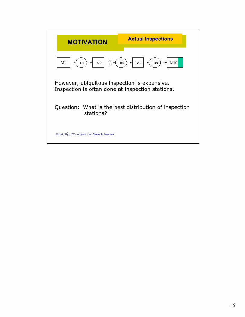
However, ubiquitous inspection is expensive. Inspection is often done at inspection stations.

Question: What is the best distribution of inspection stations?

17


Find the best way to achieve high quality with low cost by bringing quality control and material flow control together.

Develop a conceptual and computational tool which avoids conflict between productivity and quality. The tool will efficiently assess quality and throughput simultaneously.

RESEARCH RESEARCH OBJECTIVEOBJECTIVE

Mission

18


We choose a continuous material analytical modelbecause

Considerably less computation required time than simulation-> Larger searchable design space Same inputs always give same outputs

->Easy to evaluate reliable direction for improvementContinuous optimization is much easier than discrete optimization.

But…

Tough to develop. Approximate.

Research DirectionResearch Direction Analytic or Simulation?

19


Research PlanResearch Plan Big picture

1. Immediate Research PlanCharacterization2M 1BLong line decomposition

2. Long term possible research tasksOptimizationCase study for PSA

3. Ultimate GoalRedesign factory layouts.Improving inspection policiesRevamping material flow controlsSAVE BIG MONEY

20


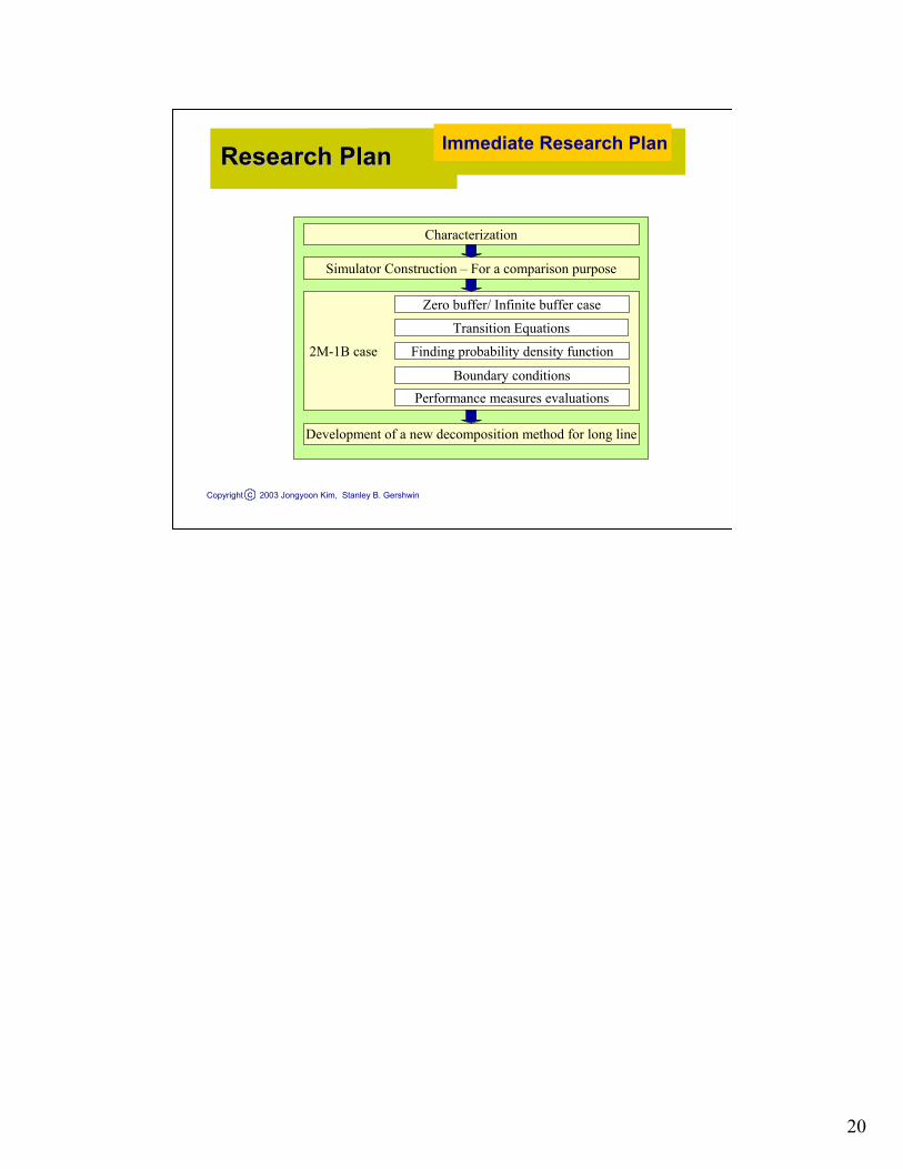
Characterization

Simulator Construction – For a comparison purpose

Development of a new decomposition method for long line

2M-1B case

Zero buffer/ Infinite buffer case

Transition Equations

Finding probability density function

Boundary conditionsPerformance measures evaluations

Research PlanResearch Plan Immediate Research Plan

21


Model DescriptionModel Description Quality

Assignable Variation: variation due to a specific, identifiable cause which changes the process mean.

Random Variation: variation that is inherent in the design of the process and cannot be removed.

Two sources of process variation

d

Meand

Tool Change

Assignable Variation

Random Variation

In this research, we focus on Assignable Variation.

22


REVIEWREVIEW Quality Failures

Common Cause Variation: random variation that is inherent in the design of the process and cannot be removed.

Assignable Cause Variation: variation due to a specific, identifiable cause.

Two kinds of process variation

Two types of quality failuresBernoulli-type: quality failure due to common cause of

variation-> quality of each part is independent of others.

Markovian-type: quality failure due to assignable cause of variation.-> Once a bad part is produced, all the subsequent parts will be bad until the operation is repaired.

In quality literatures, there are two different kinds of process variation.

Common cause variation is random variation that is inherent in the design of the process and can not be removed.

On the other hand, assignable cause variation is variation due to a specific identifiable cause.

We defined two extreme kinds of quality failures, based on the characteristics of variations that cause the failures.

The Bernoully-type quality failures are those caused by common cause variation. Therefore the quality of each part is independent of the others. Such failures occur often when an operation is sensitive to environmental perturbations or the operation uses a new technology that is difficult to control. The occurrence of a bad part implies nothing about the quality of future parts.

The Markovian type quality failures are those caused by assignable cause variations. Therefore a quality failure only happens after a change occurs in the machine. For the simplicity, in that case, once a bad part is produced, all subsequent parts will be bad until the machine is repaired.

Of course, there can be failures which is a mixture of Bernoulli - type and Markovian - type.

23


Objective – Capture important features but try to be simple!

1 -1

0

0’

pp

r

rgf

r

01 -1

p

r

g f

•Each machine can produce ‘good’ or ‘bad’ parts•Each machine has inspection

• How many states do we need? -> as few as possible!

Characterization Model DescriptionModel Description

State of One Machine

0’’

24


1 -1 0

p

g f

r

Each machine has 3 states

•State 1:Machine is producing non-defective parts.

•State –1: Machine is producing defective parts but the operator doesn’t know it.

•State 0: Machine is not operating

State of One Machine

Model DescriptionModel Description Characterization

25


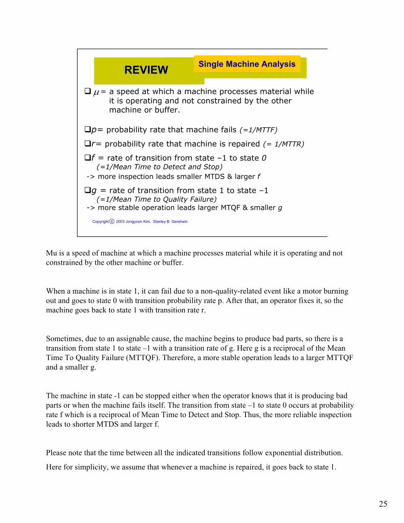
= a speed at which a machine processes material while it is operating and not constrained by the other machine or buffer.

p= probability rate that machine fails (=1/MTTF)

r= probability rate that machine is repaired (= 1/MTTR)

f = rate of transition from state –1 to state 0(=1/Mean Time to Detect and Stop)

-> more inspection leads smaller MTDS & larger f

g = rate of transition from state 1 to state –1 (=1/Mean Time to Quality Failure)

-> more stable operation leads larger MTQF & smaller g

REVIEWREVIEW Single Machine Analysis

µ

Mu is a speed of machine at which a machine processes material while it is operating and not constrained by the other machine or buffer.

When a machine is in state 1, it can fail due to a non-quality-related event like a motor burning out and goes to state 0 with transition probability rate p. After that, an operator fixes it, so the machine goes back to state 1 with transition rate r.

Sometimes, due to an assignable cause, the machine begins to produce bad parts, so there is a transition from state 1 to state –1 with a transition rate of g. Here g is a reciprocal of the Mean Time To Quality Failure (MTTQF). Therefore, a more stable operation leads to a larger MTTQF and a smaller g.

The machine in state -1 can be stopped either when the operator knows that it is producing bad parts or when the machine fails itself. The transition from state –1 to state 0 occurs at probability rate f which is a reciprocal of Mean Time to Detect and Stop. Thus, the more reliable inspection leads to shorter MTDS and larger f.

Please note that the time between all the indicated transitions follow exponential distribution.

Here for simplicity, we assume that whenever a machine is repaired, it goes back to state 1.

26


State of 2M1B

M 1 M 2B 1

),,,( 21 ααyxState Definition

x : total amount of material at B1

y : amount of defective material at B1

1α : status of machine 1 (1,-1,0)


•Blockage of machine 1 and starvation of machine 2 are dependent on x and independent of y.

•Inspection at Machine 2 can trigger state change at machine 1.

Model DescriptionModel Description Characterization

27


Buffer Size

Prod

uctio

n R

ate

Zero Buffer

Infinite Buffer

Finite Buffer

2M1B Special Cases

Develop formulas with special cases: zero buffer and infinite buffer cases.

Results are very good.

Infinite Buffer Case

Zero Buffer Case

REVIEWREVIEW

Case # Pe(A) Pe(S) % Difference1 0.657 0.662 -0.73%2 0.620 0.627 -1.15%3 0.614 0.621 -1.03%4 0.529 0.534 -0.99%5 0.480 0.484 -0.77%6 0.647 0.651 -0.57%7 0.706 0.712 -0.91%8 1.377 1.526 -9.79%9 0.706 0.711 -0.77%

10 1.377 1.380 -0.22%

Case # Pe(A) Pe(S) % Difference1 0.762 0.761 0.17%2 0.708 0.708 0.00%3 0.657 0.657 -0.06%4 0.577 0.580 -0.50%5 0.527 0.530 -0.42%6 0.745 0.745 0.01%7 0.762 0.760 0.30%8 1.524 1.522 0.14%9 0.762 0.762 0.01%

10 1.524 1.526 -0.13%

As a warming-up, special 2M1B cases which are zero buffer case and infinite buffer case were studied.

The comparison of results from the developed formulas and the simulation show very good agreement.

28


9 transition equations are derived),,1,0(),,0,1(),,1,1()(),,1,1(),,1,1()(),,1,1(

1222112

12 yxfryxfryxfgpgpy

yxfx

yx

yxft

yxf+++++−

∂∂

+∂

∂−=

∂∂ µµµ

),,0,0(),,1,1(),,0,1()(),,0,1(),,1,1(),,0,1(1221112 yxfryxffyxfrgp

xyxfyxfp

tyxf

+−+++−∂

∂−=

∂∂ µ

),,1,0(),,1,1()(),,1,1(),,1,1()(),,1,1(),,1,1(1211

2122 yxfryxffgp

yyxf

xy

xyxfyxfg

tyxf

−+−++−∂−∂

+∂−∂

−+=∂−∂ µµµ

),,1,1(),,0,0(),,1,0()(),,1,0(),,1,0(),,1,1(),,1,0(12221

221 yxffyxfryxfgpr

yyxf

xy

xyxfyxfp

tyxf

−++++−∂

∂+

∂∂

+=∂

∂ µµ

),,0,1(),,1,0(),,0,0()(),,1,0(),,0,1(),,0,0(122121 yxffyxffyxfrryxfpyxfp

tyxf

−+−++−+=∂

∂

),,1,1(),,1,0(),,1,0(),,1,0()(),,1,0(),,1,1(),,1,0(1

222121 yxffyx

xy

xyxfyxffryxfgyxfp

tyxf

−−+−+∂−∂

+−+−+−=∂−∂ µµ

),,0,1(),,1,1()(),,1,1()(),,1,1()(),,1,1(),,1,1(21

2121221 yxfr

yyxf

xy

xyxfyxffgpyxfg

tyxf

−+∂

−∂−+

∂−∂

−+−++−=∂

−∂ µµµµ

),,1,1(),,1,1(),,0,1()(),,0,1(),,0,1(),,0,1(),,0,1(2212111 yxffyxfpyxffr

yyxf

xyxfyxfg

tyxf

−−+−+−+−∂

−∂−

∂−∂

−=∂

−∂ µµ

),,1,1()(),,1,1()(),,1,1()(),,1,1(),,1,1(),,1,1(211

21221 yxfff

yyxf

xy

xyxfyxfgyxfg

tyxf

−−+−∂−−∂

−+∂−−∂

−+−+−=∂−−∂ µµµµ

Model DescriptionModel Description2M1B Internal Transition

Equations

29


The transition equations are linear partial differential equations in t,x,y with coefficients that are nonlinear functions or x and y.

),,( 21 ααx

Unlikely to be solved

Facts• Starvation and Blockage of machines are independent of y.• Average value of y can be calculated from other formulations.

Redefine the 2M1B state as


Equations

30


1 2( , , )x α αState Definition

x : total amount of material at B



2M1B

No part is scrapped: defective parts are marked and reworked later.

REVIEWREVIEW

M 1 M 2B

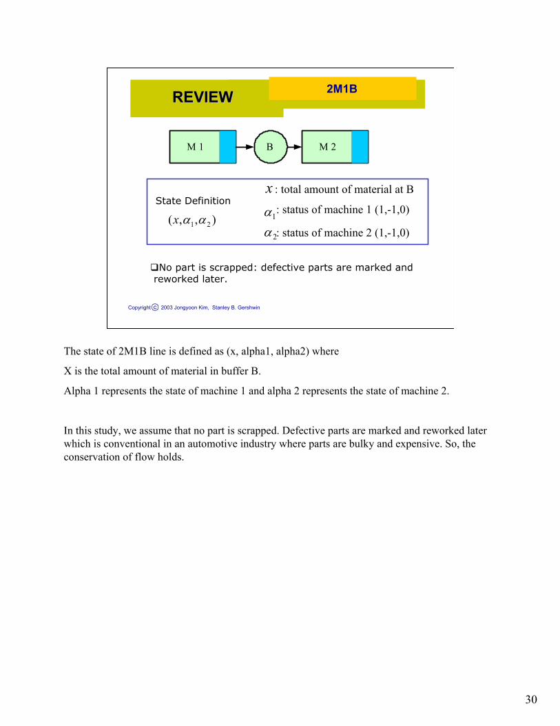
The state of 2M1B line is defined as (x, alpha1, alpha2) where

X is the total amount of material in buffer B.

Alpha 1 represents the state of machine 1 and alpha 2 represents the state of machine 2.

In this study, we assume that no part is scrapped. Defective parts are marked and reworked later which is conventional in an automotive industry where parts are bulky and expensive. So, the conservation of flow holds.

31


2M1B Finite Buffer Case

Finite buffer case:

Approach: Develop Markov process model;

write and solve transition equations and boundary equations.

When buffer B is neither empty nor full the behavior is described by differential equations with probability density function f(x,α1,α2).

When buffer B is either empty or full, the behavior is described by boundary equations with probability mass functions P(0,α1,α2), P(N,α1,α2).

REVIEWREVIEW

In finite buffer case, we need to develop Markov process model to analyze performance measures.

When the buffer B is neither empty nor full, its behavior is described by differential equations with probability density function f(x,a1,a2) since buffer level can change only a small amount during a short time interval.

When buffer B is either empty or full, the behavior is described by boundary equations with probability masses.

32


9 transition equations for f(x,α1,α2) are derived

2 1 1 1 2 2 2 1( ,1,1) ( ,1,1)( ) ( ) ( ,1,1) ( ,1,0) ( ,0,1)f x f x p g p g f x r f x r f x

t xµ µ∂ ∂

= − − + + + + +∂ ∂

2 1 1 1 2 2 1( ,1,0) ( ,1,0)( ,1,1) ( ) ( ,1,0) ( ,1, 1) ( ,0,0)f x f xp f x p g r f x f f x r f x

t xµ∂ ∂

= − − + + + − +∂ ∂

2 2 1 1 1 2 1( ,1, 1) ( ,1, 1)( ,1,1) ( ) ( ) ( ,1, 1) ( ,0, 1)f x f xg f x p g f f x r f x

t xµ µ∂ − ∂ −

= + − − + + − + −∂ ∂

1 2 1 2 2 2 1( ,0,1) ( ,0,1)( ,1,1) ( ) ( ,0,1) ( ,0,0) ( , 1,1)f x f xp f x r p g f x r f x f f x

t xµ∂ ∂

= + − + + + + −∂ ∂

1 2 1 2 2 1( ,0,0) ( ,1,0) ( ,0,1) ( ) ( ,0,0) ( ,0, 1) ( , 1,0)f x p f x p f x r r f x f f x f f x

t∂

= + − + + − + −∂

1 2 1 2 2 1( ,0, 1) ( ,0, 1)( ,1, 1) ( ,0,1) ( ) ( ,0, 1) ( , 1, 1)f x f xp f x g f x r f f x f f x

t xµ∂ − ∂ −

= − + − + − + + − −∂ ∂

1 2 2 1 2 1 2( , 1,1) ( , 1,1)( ,1,1) ( ) ( , 1,1) ( ) ( , 1,0)f x f xg f x p g f f x r f x

t xµ µ∂ − ∂ −

= − + + − + − + −∂ ∂

1 1 2 1 2 2( , 1,0) ( , 1,0)( ,1,0) ( ) ( , 1,0) ( , 1,1) ( , 1, 1)f x f xg f x r f f x p f x f f x

t xµ∂ − ∂ −

= − − + − + − + − −∂ ∂

1 2 2 1 1 2( , 1, 1) ( , 1, 1)( ,1, 1) ( , 1,1) ( ) ( ) ( , 1, 1)f x f xg f x g f x f f f x

t xµ µ∂ − − ∂ − −

= − + − + − − + − −∂ ∂

REVIEWREVIEW2M1B Internal


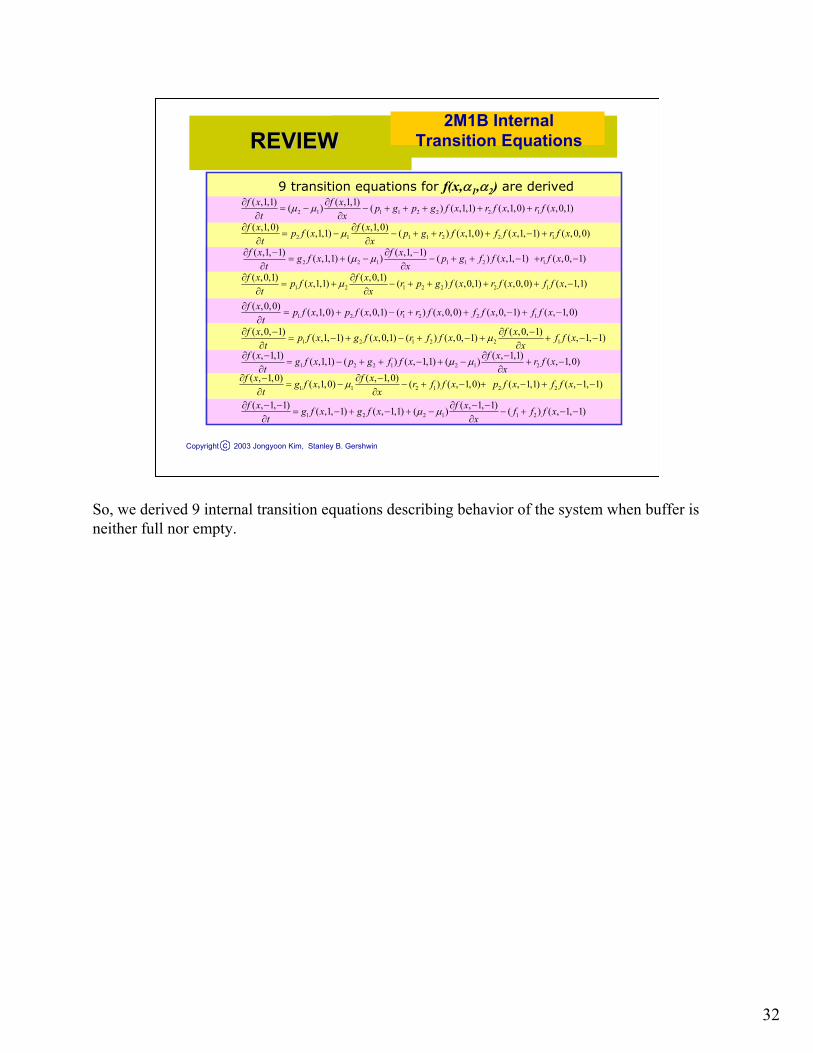
So, we derived 9 internal transition equations describing behavior of the system when buffer is neither full nor empty.

33


)()(),,( 221121 αααα λ GGexf x=Assume a solution in a form of .

After much mathematical manipulation, the equations are

simplified into 2 equations and 2 unknowns.

It turns out that there are multiple roots

depending on machine parameters. (3 to 7 roots)

A general solution to the transition equations is a linear

combination of the roots.

REVIEWREVIEWSolution to Internal


1 2 1 1 2 2( , , ) ( ) ( )i x i iif x e G Gλα α α α=

1 2 1 1 2 21

( , , ) ( ) ( )i

RNx i i

ii

f x c e G Gλα α α α=

=∑

And by assuming a solution form of this and a lot of mathematical manipulation, we could simplify the 9 equations and 7 unknowns to 2 equations and 2 unknowns.

The equations are high order equations in which no analytic solution is possible. Therefore, we developed an algorithms to solve these equations.

It turned out that there are multiple roots depending on machine parameters. Therefore, the general solution is a linear combination of the roots found from the algorithm.

34


)()(),,( 221121 αααα λ GGexf x=Assume that Then, the transition equations in steady state become

0)1()0()0()1()}1()1()(){( 21121221221112 =+++++−− GGrGGrGGgpgpλµµ

0)0()0()1()1()1()1()0()1()}({ 211212212212111 =+−+++++− GGrGGfGGpGGrgpλµ

0)1()0()1()1()1()1()}(){( 2112122121112 =−++−++−− GGrGGgGGfgpλµµ

0)1()1()0()0()1()1()1()0()}({ 211212211212212 =−+++++− GGfGGrGGpGGgprλµ

0)0()1()1()0()0()0()()1()0()0()1( 2112122121212211 =−+−++−+ GGfGGfGGrrGGpGGp

0)1()1()1()0()1()1()1()0()}({ 21121221121212 =−−++−+−+− GGfGGgGGpGGfrλµ

0)0()1()1()1()1()1()}(){( 2122112112212 =−++−++−− GGrGGgGGfgpλµµ

0)1()1()1()1()0()1()0()1()}({ 21221221121121 =−−+−++−++− GGfGGpGGgGGfrλµ

0)1()1()1()1()1()1()}(){( 212211212112 =−+−+−−+−− GGgGGgGGffλµµ


Equations

35


021 =Γ+Γ

212 Ψ+Γ=− λµ 121 Ψ+Γ=λµ

2121 )( Ψ+Ψ=− λµµ 2121 )( Θ+Θ=− λµµ

121 Θ+Γ=λµ 212 Θ+Γ=− λµ

1221 )( Θ+Ψ=− λµµ 2121 )( Θ+Ψ=− λµµ

)0()1(

)0()1(

i

iii

i

iii G

GfrGGp −

+−=Γ

)1()0(

i

iiiii G

Grgp +−−=Ψ)1(

)1(−

+−=Θi

iiii G

Ggf

If we define

Then, 9 transitionequations become

Model DescriptionModel Description2M1B Transition

Equations (5)

36


021 =Γ+Γ 1 1 1 1 1 2 2 2 2 2( )pY r f Z p Y r f Z M− + =− − + =

1 1 2 21 1 1 1 2 2 2 2

1 1 2 2,r Y r Yp g f g p g f gY Z Y Z− − + = − + − − + = − +

1 21 1 2 2

1 11 1(1 ) (1 ) NY Z Y Zµ µ+ = + =+ +

In addition to that, we already have


Equations

And introduce two parameters: M, N

(1) ( 1),(0) (0)

i ii i

i i

G GY ZG G

−= =Define

37


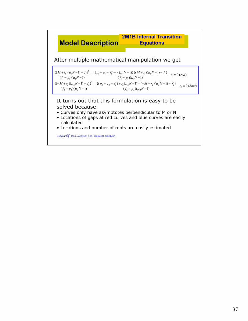
After multiple mathematical manipulation we get

21 1 1 1 1 1 1 1 1 1 1

11 1 1 1 1 1

22 2 2 2 2 2 2 2 2 2 2

22 2 2 2 2 2

{( )( 1) } {( ) ( 1)}{( )( 1) }0 ( )

( )( 1) ( )( 1)

{( )( 1) } {( ) ( 1)}{( )( 1) }0 ( )

( )( 1) ( )( 1)

M r N f p g f r N M r N fr red

f p N f p N

M r N f p g f r N M r N fr blue

f p N f p N

µ µ µµ µ

µ µ µµ µ

+ − − + − + − + − −− − =

− − − −

− + − − + − + − − + − −− − =

− − − −

It turns out that this formulation is easy to be solved because• Curves only have asymptotes perpendicular to M or N• Locations of gaps at red curves and blue curves are easily

calculated • Locations and number of roots are easily estimated


Equations

38



Equations

39


From the characterization of red curves and blue curveswhat we found are:

•There are 3 roots at the top•There are no roots at the bottom•There are maximum 4 roots at RHS or LHS•If there are any roots at RHS, then there are no roots at LHS

and vice versa

Root finding

Based on the characterization of the curves, a special algorithm to find all the roots is developed.

Model DescriptionModel Description2M1B Transition

Equations (10)

40


2M1B Boundary Equations

1 1 2 2 1( ) (0,1,1) (0,0,1) 0b bp g p g P r P− + + + + =

2 1 1 2 1(0,1,1) ( ) (0,1, 1) (0,0, 1) 0b bg P p g f P r P− + + − + − =

1 1 2 1 2(0,1,1) (0,0,1) (0,0,1) (0, 1,1) (0,0,0) 0p P r P f f P r Pµ− + + − + =

1 1 2 1(0,1, 1) (0,0, 1) (0,0, 1) (0, 1, 1) 0p P r P f f Pµ− − − + − + − − =

1 1 2 2(0,1,1) ( ) (0, 1,1) 0b bg P f p g P− + + − =

1 2 1 2(0,1, 1) (0, 1,1) ( ) (0, 1, 1) 0b bg P g P f f P− + − − + − − =

How to determine coefficients in probability density functionsand probability masses ?

ic

1 2 1 2(0, , ), ( , , )P P Nα α α α

22 Boundary equations are derived for case and solved.1 2µ µ=

…

REVIEWREVIEW

To determine coefficients in probability density functions and probability masses, we derived 22 boundary equations for mu1 = mu2 case and solved.

41


After finding all of probability densities and masses,

Total production rate is calculated from

2

1

11 2 2 2 2

1,0,1 0

2 1 11,0,1

[ { ( , 1, ) ( ,1, )} (0,1, ) (0, 1, )]

{ ( , ,1) ( , , 1)}

N

T TP P f x f x dx P P

P N P Nα

α

µ α α α α

µ α α=−

=−

= = − + + + −

+ + −

∑ ∫

∑

REVIEWREVIEW2M1B

Performance Measures

Average inventory is expressed as

1 2

1 2 1 21,0,1 1,0,1 0

( , , ) ( , , )N

x xf x dx NP Nα α

α α α α=− =−

⎡ ⎤= +⎢ ⎥

⎣ ⎦∑ ∑ ∫

After finding all the probability masses and density, we can calculate such performance measures as

The total production rate which is a production rate of good and bad parts.

Average inventory at buffer B.

And the effective production rate which is a production rate of good parts.

42


1 2E E

E TT T

P PP PP P= × ×

where2

11 2 2 2

1,0,1 0

[ ( ,1, ) (0,1, )] { ( ,1, 1) ( ,1,1)}N

EP f x dx P P N P Nα

µ α α µ=−

= + + − +∑ ∫

1

22 1 1 1

1,0,1 0

[ ( , ,1) ( , ,1)] { (0, 1,1) (0,1,1)}N

EP f x dx P N P Pα

µ α α µ=−

= + + − +∑ ∫

REVIEWREVIEW2M1B

Performance Measures

Effective production rate is calculated from

After finding all of probability densities and masses,

43


Preliminary ResultPreliminary Result 2M1B Validation

Solution for 2M1B with equal production rate case is found and validated through comparison with simulation.

Case # PR(Analytic) PR(Sim) %Difference Inv(Analytic) Inv(Sim) %Difference1 0.806 0.808 -0.25% 2.500 2.619 -4.53%2 0.855 0.858 -0.37% 25.000 24.883 0.47%3 0.936 0.938 -0.23% 4.709 4.989 -5.60%4 0.944 0.946 -0.22% 12.654 12.757 -0.81%5 0.909 0.911 -0.19% 2.781 2.832 -1.81%6 0.922 0.924 -0.24% 9.213 9.318 -1.13%7 0.909 0.910 -0.07% 2.220 2.321 -4.39%8 0.925 0.926 -0.18% 7.242 7.080 2.30%9 0.840 0.843 -0.38% 20.020 20.149 -0.64%

10 0.763 0.767 -0.49% 4.983 5.110 -2.48%

44


2M1B Validation (1)

Analytic solution for 2M1B with case is found and validated through comparison with simulation.

Average absolute error = 0.73%

Effective production rate estimation Average inventory estimation

Average absolute error = 2.75%

-10.00%

-8.00%

-6.00%

-4.00%

-2.00%

0.00%

2.00%

4.00%

6.00%

8.00%

10.00%

1 4 7 10 13 16 19 22 25 28 31 34 37 40 43 46 49

Case Number

% e

rror

of

P E

-10.00%

-8.00%

-6.00%

-4.00%

-2.00%

0.00%

2.00%

4.00%

6.00%

8.00%

10.00%

1 4 7 10 13 16 19 22 25 28 31 34 37 40 43 46 49

Case Number

% e

rror

of

Inv

REVIEWREVIEW

1 2µ µ=

Performance measures from the analytic model when the two machine speeds are the same are compared with results from the simulation.

Both the effective production rate and average inventory show good agreements.

45


Boundary Equations

26 Boundary equations are derived and solved.

22M1B with M1B with 1 2µ µ≠

1 2 2(0,1,0) (0,1,1) (0,1, 1)b bf p P f Pµ = + −

1 2 2(0, 1,0) (0, 1,1) (0, 1, 1)b bf p P f Pµ − = − + − −

2 ( ,0,1) 0f Nµ =

2 ( ,0, 1) 0f Nµ − =

2 1 2( ) ( ,1,1) ( ,1,0)f N r P Nµ µ− =

2 1 2( ) ( , 1,1) ( , 1,0)f N r P Nµ µ− − = −

1 1 2 2 2 1 1( ) (0,1,1) ( ) (0,1,1) (0,0,1) 0b bp g p g P f r Pµ µ− + + + + − + =

…

Now new stuff.

After the first thesis committee meeting, I finished constructing boundary equations for different machine speeds.

In these cases, 26 (rather than 22) equations are need for each of mu1 > mu2 case and mu1 < mu2 case.

46


22M1B with M1B with 1 2µ µ≠ 2M1B Validation (2)

-10.00%

-8.00%

-6.00%

-4.00%

-2.00%

0.00%

2.00%

4.00%

6.00%

8.00%

10.00%

1 4 7 10 13 16 19 22 25 28 31 34 37 40 43 46 49

Case Number

% e

rror

of

P E

Analytic solution for 2M1B with case is found and validated through comparison with simulation.

-10.00%

-8.00%

-6.00%

-4.00%

-2.00%

0.00%

2.00%

4.00%

6.00%

8.00%

10.00%

1 4 7 10 13 16 19 22 25 28 31 34 37 40 43 46 49

Case Number

% e

rror

of

Inv

Effective production rate estimation

1 2µ µ≠

Average inventory estimation

Average absolute error = 0.68% Average absolute error = 3.41%

The boundary equations were solved and the performance measures were compared with results from the simulation.

Again, we can see good agreements in the estimate of effective production rate and average inventory.

47


Preliminary ResultPreliminary ResultQuality Information

Feedback

M 1 M 2

Inspection @ M2 notify M1 isproducing bad parts

Inspection @ M1 notify M1 isproducing bad parts

Downstream machines can detect defective parts made by an upstream machine and notify the operator at the machine.

Quality Information Feedback

48


Preliminary ResultPreliminary ResultQuality Information

Feedback

If there is quality information feedback, the yield of the system depends on the time gap between making a defect and identifying the defect.

System yield is a function of buffer size: A smaller buffer increases system yield since lower inventory level leads to a smaller the time gap.

49


Preliminary ResultsPreliminary ResultsQuality Information

Feedback

0 5 10 15 20 250.72

0.73

0.74

0.75

0.76

0.77

0.78

0.79

0.8

Buffer Size

Pro

duct

ion

Rat

e

Pr w/o feedbackPr w/ feedback

0 5 10 15 20 250.65

0.66

0.67

0.68

0.69

0.7

0.71

0.72

0.73

0.74

Buffer SizeE

ffect

ive P

rodu

ctio

n R

ate

ePr w/o feedbackePr w/ feedback

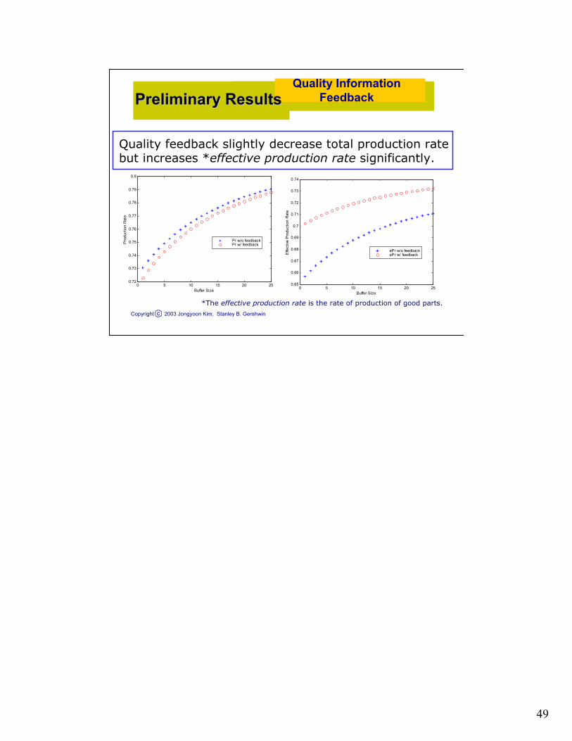
*The effective production rate is the rate of production of good parts.

Quality feedback slightly decrease total production rate but increases *effective production rate significantly.

50


Preliminary ResultsPreliminary ResultsHow to Increase

Quality

0 50 100 150 200 250 300 350 400 450 5000.3

0.4

0.5

0.6

0.7

0.8

0.9

1

Mean Time To Defect

Effe

ctiv

e P

rodu

ctio

n R

ate

0 20 40 60 80 100 120 140 160 180Mean Time To Identify

0.1

0.2

0.3

0.4

0.5

0.6

0.7

0.8

Effe

ctiv

e P

rodu

ctio

n R

ate

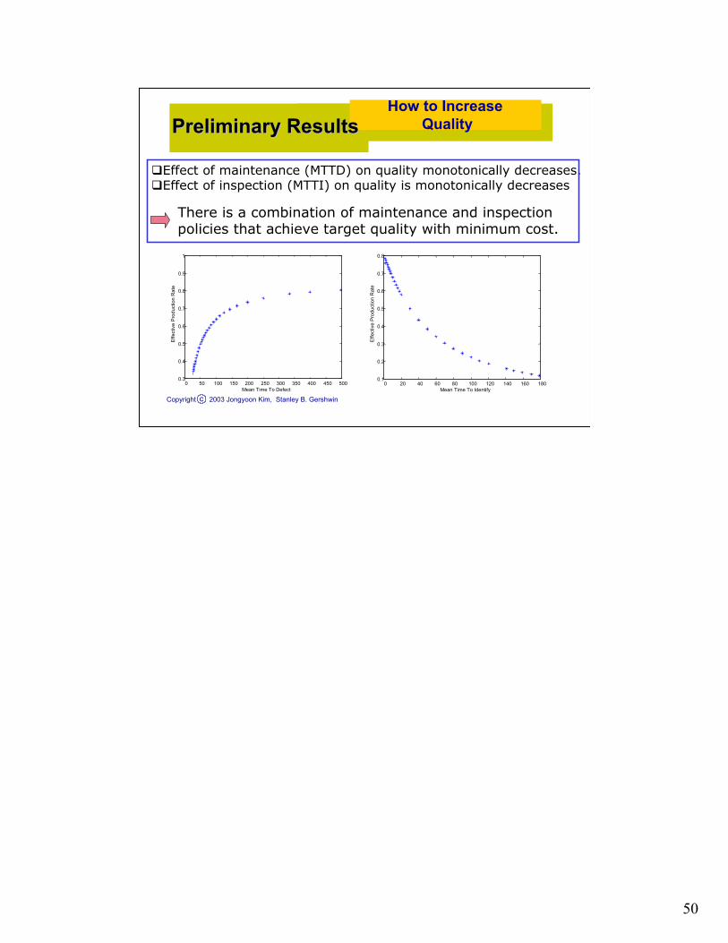
Effect of maintenance (MTTD) on quality monotonically decreases.Effect of inspection (MTTI) on quality is monotonically decreases

There is a combination of maintenance and inspection policies that achieve target quality with minimum cost.

51


Preliminary ResultsPreliminary ResultsHow to increase

productivity

In some situations, increasing inspection reliability is more effective than increasing buffer size to boost productivity.

0 5 10 15 20 25 30 35 400.63

0.635

0.64

0.645

0.65

0.655

0.66

Buffer Size

Effe

ctiv

e P

rodu

ctio

n R

ate

0 5 10 15 20 25 30 35 400.885

0.89

0.895

0.9

0.905

0.91

0.915

0.92

0.925

0.93

Buffer SizeE

ffect

ive

Pro

duct

ion

Rat

e

52


Preliminary ResultPreliminary ResultHow to increase

productivity?

0 5 10 15 20 25 30 35 400.77

0.78

0.79

0.8

0.81

0.82

0.83

0.84

0.85

Buffer Size

Effe

ctiv

e P

rodu

ctio

n R

ate

0 5 10 15 20 25 30 35 400.24

0.25

0.26

0.27

0.28

0.29

0.3

0.31

0.32

0.33

Buffer Size

Effe

ctiv

e P

rodu

ctio

n R

ate

In some situations, increasing machine stability is more effective than increasing buffer size to enhance productivity.

53



Downstream machines can detect defective parts made by an upstream machine and notify the operator at the machine.

REVIEWREVIEW

M 1 M 2

Inspection @ M2

Inspection @ M1

System yield is a function of buffer size: A smaller buffer increases system yield since lower inventory level leads to a early detection of quality failures.

Quality information feedback is captured by modifying f.

Due to cost of inspection, factories are often designed so that multiple inspections are performed at a small number of stations. In this case, inspection at downstream operations can give feedback to upstream machine. We call this quality information feedback.

In this case, the yield of a line is a function of the size of buffers. This is because when buffers are larger, more material accumulates between an operation and the inspection of that operation. All such material will be defective if the Markovian type quality failure take place. Therefore smaller buffer may increase system yield.

54


0 5 10 15 20 250.65

0.7

0.75

0.8

Buffer Size

Effe

ctiv

e P

rodu

ctio

n R

ate Without feedback

With feedback

0 5 10 15 20 250.65

0.7

0.75

0.8

Without feedbackWith feedback

0 5 10 15 20 250.65

0.7

0.75

0.8


0 5 10 15 20 250.65

0.7

0.75

0.8

Buffer Size

Tota

l pro

duct

ion

Rat

e


0 5 10 15 20 250.65

0.7

0.75

0.8


0 5 10 15 20 250.65

0.7

0.75

0.8



Quality feedback results in more effective production rate and less total production rate.

Increase of buffer size is beneficial contrary to TPS.

MFG. SYSTEM MFG. SYSTEM BEHAVIORBEHAVIOR

Let’s talk about

55



The effective production rate may decrease as the buffer size increases when•M1 is faster than M2 and quality feedback exists.•M1 produces bad parts frequently.•Inspection at M1 is poor and inspection at M2 is good.

This is a case when inventory reduction is good as TPS advocates.

Harmful Buffer Case

0 5 10 15 20 25 30 35 400.3

0.35

0.4

0.45

0.5

0.55

0.6

0.65

0.7

0.75

0.8

Buffer Size

Effe

ctiv

e Pr

oduc

tion

Rat

e


56


0 0.1 0.2 0.3 0.4 0.5 0.6 0.7 0.8 0.9 10.1

0.2

0.3

0.4

0.5

0.6

0.7

0.8

0.9

f

Effe

ctiv

e Pr

oduc

tion

Rate

0 0.1 0.2 0.3 0.4 0.5 0.6 0.7 0.8 0.9 10.1

0.2

0.3

0.4

0.5

0.6

0.7

0.8

0.9

fEf

fect

ive

Prod

uctio

n R

ate

0.398

0.560

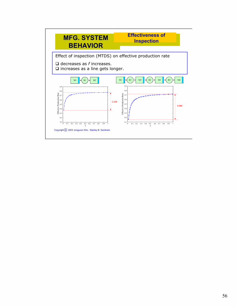
M1 B1 M2 M1 B1 M2 B2 M3 B3 M4

Effect of inspection (MTDS) on effective production rate

decreases as f increases.increases as a line gets longer.


Effectiveness of Inspection

57



Effectiveness of Operation Stabilization

0 50 100 150 200 250 300 350 400 450 5000

0.1

0.2

0.3

0.4

0.5

0.6

0.7

0.8

0.9

MTQF

Effe

ctiv

e Pr

oduc

tion

Rat

e

0 50 100 150 200 250 300 350 400 450 5000

0.1

0.2

0.3

0.4

0.5

0.6

0.7

0.8

0.9

MTQF

Effe

ctiv

e Pr

oduc

tion

Rat

e

0.609

0.701

Effect of machine stabilization (MTQF) on effective production rate

decreases as MTQF increases.increases as a line gets longer.

M1 B1 M2 M1 B1 M2 B2 M3 B3 M4

58


How to increaseproductivity

In some situations, increasing inspection reliability is more effective than increasing buffer size to boost productivity.

0 5 10 15 20 25 30 35 400.5

0.55

0.6

0.65

0.7

0.75

0.8

Buffer Size

Effe

ctiv

e Pr

oduc

tion

Rat

e

MTDS = 20MTDS = 10MTDS = 2


59


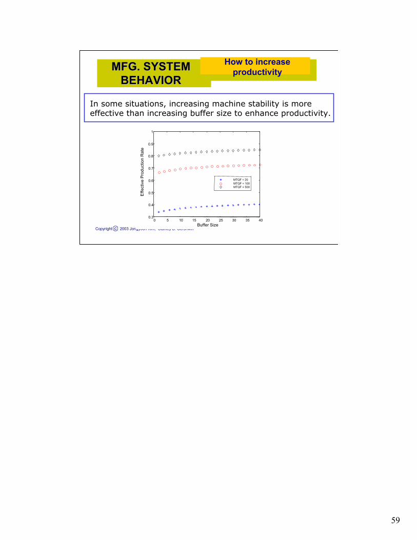
How to increaseproductivity

In some situations, increasing machine stability is more effective than increasing buffer size to enhance productivity.

0 5 10 15 20 25 30 35 400.3

0.4

0.5

0.6

0.7

0.8

0.9

1

Buffer Size

Effe

ctiv

e Pr

oduc

tion

Rat

e

MTQF = 20MTQF = 100MTQF = 500


60


LONG LINELONG LINE Extension

Longer line increases the dimension of partial differential equations used at internal transitions equations.

No good exact method known for longer lines.

It is reasonable to use approximation methods to obtain solutions for transfer lines with more than two machines.

Decomposition techniques have been successfully used for various kind of long line analysis.

Tandem long lineAssembly/disassembly lineClosed loop

The dimension of partial differential equations to describe behavior of a manufacturing system is the same as the number of buffers in the system.

So, longer line increases the dimension of the partial differential equations.

Since it is almost impossible to solve multi-dimensional partial differential equations, it does not seem to be possible to get exact solutions for long line analysis.

Therefore, approximation techniques have been used for manufacturing lines with more then two machines.

Among the approximation techniques, decomposition methods have been most successfully used for various kind of lone line analysis including tandem line, assembly/disassembly and closed loop system.

61


Decomposition TechniqueLONG LINELONG LINE

M1 B1 M2 M3 M4B2 B3

1 1 1

1 1

, ,,r p

g fµ 2 2 2

2 2

, ,,r p

g fµ 3 3 3

3 3

, ,,r p

g fµ

4 4 4

4 4

, ,,r p

g fµ

L

(1), (1), (1)(1), (1)

u u u

u u

r pg f

µ

Mu (1) B(1) L(1)Md (1)

1N

B(2) L(2)Mu (2) Md (2)

B(3) L(3)Mu (3) Md (3)

(1), (1), (1)(1), (1)

d d d

d d

r pg f

µ

Decomposition

(2), (2), (2)(2), (2)

u u u

u u

r pg f

µ2N (2), (2), (2)

(2), (2)d d d

d d

r pg f

µ

(3), (3), (3)(3), (3)

u u u

u u

r pg f

µ3N (3), (3), (3)

(3), (3)d d d

d d

r pg f

µ

1N 2N3N

The idea of decomposition method is to break k-stage lines, we call L, into k-1 2M1B line L(I) in a way that behavior of material flow through buffer B(I) of the decomposed 2M1B system is close enough to the behavior of material flow through buffer B_I at the original line.

In other words, the decomposition technique tries to determine the characteristics of the machines of each decomposed line such that on observer at the buffer B(I) can not tell whether he/she is on the original long line or the decomposed line.

Each decomposed line L(I) consists of two psudo-machines, Mu(I), and Md(I). The machine Mu(I) represent aggregate behavior of the flow up stream of buffer B_I.

And the machine Md(I) models the part of the original line L downstream of the buffer Bi.

62


Decomposition TechniqueLONG LINELONG LINE

Decomposition TechniqueDecompose the line (L) into a set of two-machine lines L(i) in a way

that performance measures of the L(i)s are close to those of the original line L.

Pseudo-machine Mu(i) models the part of the line upstream of Bi and Md(i) models the part of line downstream from Bi.

Decomposition techniques work well even though no mathematical proof is available.

Procedures

Develop equations for 10(k-1) pseudo-machine parameters for k-machine line.

Develop algorithm to solve the equations efficiently.

Since each decomposed 2M1B system has two pseudo machines and each machine has 5 parameters. (Mu, r, p, g f), we need to determine 10*(k-1) unknowns.

Therefore, we need to develop the same number of equations and algorithm to solve the equations efficiently.

63


Ubiquitous InspectionCaseLONG LINELONG LINE

Each machine has both of operational failures and quality failuresEach operation works on different features.Inspection at machine Mi can detect defective features made by Minot others.

For each decomposed line L(i), incoming parts from upstream are viewed as non-defective ones. -> gi is independent of other machine parameters: gu(i) = gi , gd(i) = gi+1

Outgoing defective parts from L(i) are not checked from inspection downstream -> fi is independent of others: fu(i) = fi , fd(i) = fi+1

The first long line analysis task we choose is a ubiquitous inspection case.

This is a case that

-Each machine has both of operational failures and quality failures.

-Each operation works on different features.

-Inspection at machine Mi can detect bad features made by machine Mi not others.

Under these assumptions,

For each decomposed line L(I), incoming parts from upstream are viewed as non defective. And also, outgoing defective parts from the decomposed line are not checked. Therefore, g_I and f_I are independent of other machine parameters.

As a result, decomposition equations for g_I are gu(I)=g_I, gd(I)=g_(I+1).

In a same way, the decomposition equations for f_I are f_u(I)=f_I, and f_d(I) = f_(I+1).

M1 M2 M3 M4B3B1 B2

64


3-state-machine /2-state-machineLONG LINELONG LINE

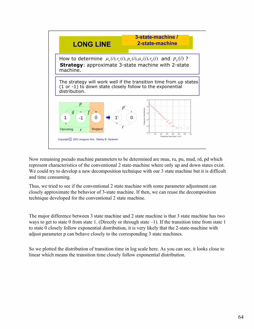
How to determine and ?Strategy: approximate 3-state machine with 2-state machine.

The strategy will work well if the transition time from up states (1 or -1) to down state closely follow to the exponential distribution.

0 100 200 300 400 500 600 70010

-5

10-4

10-3

10-2

10-1

100

Freq

uenc

y di

strib

utio

n

Transition time from 1 to 0

( ), ( ), ( ), ( ), ( )u u u d di r i p i i r iµ µ ( )dp i

Now remaining pseudo machine parameters to be determined are muu, ru, pu, mud, rd, pd which represent characteristics of the conventional 2 state-machine where only up and down states exist. We could try to develop a new decomposition technique with our 3 state machine but it is difficult and time consuming.

Thus, we tried to see if the conventional 2 state machine with some parameter adjustment can closely approximate the behavior of 3-state machine. If then, we can reuse the decomposition technique developed for the conventional 2 state machine.

The major difference between 3 state machine and 2 state machine is that 3 state machine has two ways to get to state 0 from state 1. (Directly or through state –1). If the transition time from state 1 to state 0 closely follow exponential distribution, it is very likely that the 2-state-machine with adjust parameter p can behave closely to the corresponding 3 state machines.

So we plotted the distribution of transition time in log scale here. As you can see, it looks close to linear which means the transition time closely follow exponential distribution.

1' -1 1 0 0g

p

p'

f

rr

Operating Stopped

65


-10.00%

-8.00%

-6.00%

-4.00%

-2.00%

0.00%

2.00%

4.00%

6.00%

8.00%

10.00%

1 7 13 19 25 31 37 43 49 55 61 67 73 79 85 91 97

Case Number

% e

rror

of

P E

-10.00%

-8.00%

-6.00%

-4.00%

-2.00%

0.00%

2.00%

4.00%

6.00%

8.00%

10.00%

1 7 13 19 25 31 37 43 49 55 61 67 73 79 85 91 97

Case Number

% e

rror

of

Inv


A 2-state-machine with parameter adjustments closely approximates the corresponding 3-state-machine.

LONG LINELONG LINE3-state-machine /2-state-machine

To make it sure, we conducted comparison of 2M1B systems with 3-state machine and corresponding 2 state machine ones after parameter adjustment for 100 cases.

And it turned out that the average absolute difference in the effective production rate estimation is less than 1% and the average absolute difference in the average buffer level is around 1 %.

66


Long Line ValidationLONG LINELONG LINE

-20.00%

-15.00%

-10.00%

-5.00%

0.00%

5.00%

10.00%

15.00%

20.00%

1 2 3 4 5 6 7 8 9 10 11 12 13 14 15 16 17 18 19 20

Case Number

% e

rror

of P

E

-20.00%

-15.00%

-10.00%

-5.00%

0.00%

5.00%

10.00%

15.00%

20.00%

1 2 3 4 5 6 7 8 9 10 11 12 13 14 15 16 17 18 19 20

Case Number

% e

rror

of I

nv 1

-20.00%

-15.00%

-10.00%

-5.00%

0.00%

5.00%

10.00%

15.00%

20.00%

1 2 3 4 5 6 7 8 9 10 11 12 13 14 15 16 17 18 19 20

Case Number

% e

rror

of I

nv 2

-20.00%

-15.00%

-10.00%

-5.00%

0.00%

5.00%

10.00%

15.00%

20.00%

1 2 3 4 5 6 7 8 9 10 11 12 13 14 15 16 17 18 19 20

Case Number%

err

or o

f Inv

3



Finally performance measures estimated from the decomposition technique are compared with the simulation result.

Again, we can see good agreements in the estimate of effective production rate and average buffer levels.

M1 M3 M4B1 B2M2 B3

67


UPCOMING TASKUPCOMING TASK Effective of Jidoka

Does JIDOKA (stopping the lines whenever abnormalities occur) improve quality and productivity in every case?

Hypothesis

The effectiveness of Jidoka on productivity depends on which type of quality failures (Markovian or Bernoulli) is dominant.

The effective production rate may decrease by adopting Jidokapractice when quality failures are mixture of Bernoulli and Markovian

68


FUTURE PLANFUTURE PLANNext Long Line Analysis Task

Inspection

M1 B1 M2 M3 M4B2 B3

Operational Failures + Quality Failures

Operational Failures

M1 undergoes both of quality failures and operational failures.

Other machines (M2, M3 , M4 ) have only operational failures.

Inspection takes place only at the final machine (M4)

69


FUTURE PLANFUTURE PLANNext Long Line Analysis Task

Inspection

M1 B1 M2 M3 M4B2 B3

Operational Failures + Quality Failures

Each machine has both of quality failures and operational failures.

Inspection is only at the final machine (M4) and detect bad parts made by any of upstream machines.

70


RESEARCHRESEARCHPROGRESSPROGRESS

Term Research Progress1999 - Spring 2002 Research on Toyota Production Systems .

Fall 2002 Chacterization. 2M1B model formulation.Simulation building.Infinite buffer and zero buffer validations.

Summer 2003 Internship at General MotorsProposal to General Motors for collaboration. Thesis proposal finalization.2M1B model completion.

1st committee meeting (Dec, 15th)Long line decomposition without quality feedback.Validation of the decomposition technique.

2nd committee meeting (April 7th) Study on Jidoka practice.Long line decomposition with quality feedback.Numerical experimentations and intuition building.

3rd committee meeting (late May/ early June)Possible case study at GMFinalize the research Finish thesis write up

Defense (Early September)

Summer 2004

Fall 2003

Spring 2003

Spring 2003

71


SupplementarySupplementaryNotesNotes

Input Parameters for2M1B Special Cases

Case # Mu1 Mu2 r1 r2 p1 p2 g1 g2 f1 f21 1.0 1.0 0.400 0.100 0.010 0.010 0.001 0.001 0.100 0.5002 1.0 1.0 0.100 0.100 0.010 0.010 0.001 0.001 0.100 0.5003 1.0 1.0 0.100 0.100 0.010 0.005 0.001 0.001 0.100 0.5004 1.0 1.0 0.100 0.100 0.010 0.005 0.005 0.001 0.100 0.5005 1.0 1.0 0.100 0.100 0.010 0.005 0.001 0.001 0.100 0.100

Infinite Buffer Case

Zero Buffer CaseCase # Mu1 Mu2 r1 r2 p1 p2 g1 g2 f1 f2

1 1.0 1.0 0.400 0.100 0.010 0.010 0.001 0.001 0.100 0.1002 1.0 1.0 0.100 0.100 0.010 0.010 0.001 0.001 0.100 0.1003 1.0 1.0 0.100 0.100 0.010 0.000 0.001 0.001 0.100 0.1004 1.0 1.0 0.100 0.100 0.010 0.010 0.010 0.001 0.100 0.1005 1.0 1.0 0.400 0.100 0.010 0.010 0.001 0.001 0.100 0.300

72



Case # Mu1 Mu2 r1 r2 p1 p2 g1 g2 f1 f2 N FB?1 1.0 1.0 0.100 0.100 0.005 0.005 0.010 0.010 0.100 0.100 5 N2 1.0 1.0 0.100 0.100 0.005 0.005 0.010 0.010 0.100 0.100 50 N3 1.0 1.0 0.300 0.300 0.010 0.010 0.005 0.005 0.500 0.500 10 N4 1.0 1.0 0.300 0.300 0.010 0.010 0.005 0.005 0.500 0.500 25 N5 1.0 1.0 0.300 0.200 0.010 0.010 0.005 0.005 0.500 0.500 5 N6 1.0 1.0 0.300 0.200 0.010 0.010 0.005 0.005 0.500 0.500 15 N7 1.0 1.0 0.200 0.300 0.010 0.010 0.005 0.005 0.500 0.500 5 N8 1.0 1.0 0.200 0.300 0.010 0.010 0.005 0.005 0.500 0.500 20 N9 1.0 1.0 0.100 0.100 0.010 0.010 0.005 0.005 0.200 0.200 40 Y

10 1.0 1.0 0.100 0.100 0.010 0.010 0.001 0.001 0.200 0.200 10 Y

Input Parameters for2M1B Validation

Intermediate Buffer Size Case

73



How to increase productivity (2)

Input Parameters forPreliminary Result

Mu1 r1 p1 f11 0.1 0.01 0.1

Mu2 r2 p2 f21 0.1 0.01 0.1

How to increase productivity (1)

Mu1 r1 p1 g11 0.1 0.005 0.001

Mu2 r2 p2 g21 0.1 0.005 0.001

Mu1 r1 p1 g1 f11 0.1 0.01 0.01 0.1

Mu2 r2 p2 g2 f21 0.1 0.01 0.01 0.9

Quality feedback

Increase QualityMu1 r1 p1 g1 f1

1 0.1 0.01 0.01 0.1Mu2 r2 p2 g2 f2

1 0.1 0.01 0.01 0.1

74


21 1 1 1 1 1 1 1 1 1 1

11 1 1 1 1 1

22 2 2 2 2 2 2 2 2 2 2

22 2 2 2 2 2

{( )( 1) } {( ) ( 1)}{( )( 1) } 0 ( )( )( 1) ( )( 1)

{( )( 1) } {( ) ( 1)}{( )( 1) } 0 ( )( )( 1) ( )( 1)

M r N f p g f r N M r N f r redf p N f p N

M r N f p g f r N M r N f r bluef p N f p N

µ µ µµ µ

µ µ µµ µ

+ − − + − + − + − −− − =

− − − −

− + − − + − + − − + − −− − =

− − − −

After much mathematical manipulation.the 9 equations and 7 unknowns are simplified to

where1 1 2 2

1 1 1 2 2 21 1 2 2

(1) ( 1) (1) ( 1)( )(0) (0) (0) (0)

G G G Gp r f p r f MG G G G

− −− + =− − + =

1 1 2 21 2

1 1 2 21

1 1 1 1(1 ) (1 )(1) ( 1) (1) ( 1)(0) (0) (0) (0)

NG G G GG G G G

µ µ+ = + =

− −+ +

Simplified Internal Transition Equations SUPPLEMENTARYSUPPLEMENTARY

NOTESNOTES

75


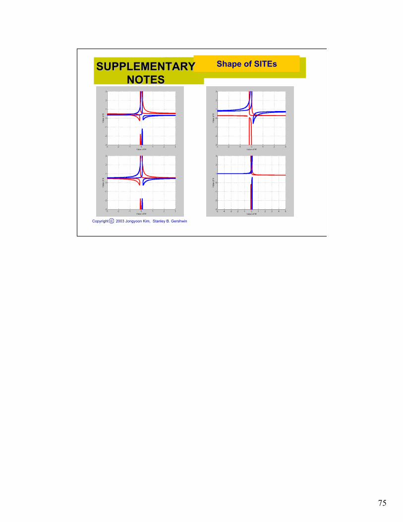
Shape of SITEsSUPPLEMENTARYSUPPLEMENTARYNOTESNOTES

76


SUPPLEMENTARYSUPPLEMENTARYNOTESNOTES

Input Parameters for2M1B Special Cases

Case # Mu1 Mu2 r1 r2 p1 p2 g1 g2 f1 f21 1 1 0.1 0.1 0.01 0.01 0.01 0.01 0.2 0.22 1 1 0.3 0.3 0.005 0.005 0.05 0.05 0.5 0.53 1 1 0.2 0.05 0.01 0.01 0.01 0.01 0.2 0.24 1 1 0.1 0.1 0.05 0.005 0.01 0.01 0.2 0.25 1 1 0.1 0.1 0.01 0.01 0.05 0.005 0.2 0.26 1 1 0.1 0.1 0.01 0.01 0.01 0.01 0.5 0.17 2 1 0.1 0.1 0.01 0.01 0.01 0.01 0.2 0.28 3 2 0.1 0.1 0.01 0.01 0.01 0.01 0.2 0.29 1 2 0.1 0.1 0.01 0.01 0.01 0.01 0.2 0.210 2 3 0.1 0.1 0.01 0.01 0.01 0.01 0.2 0.2

77


Input Parameters forPreliminary Results

Mu1 r1 p1 g1 f11 0.1 0.01 0.01 0.1

Mu2 r2 p2 g2 f21 0.1 0.01 0.01 0.9

Quality Feedback

Harmful Buffer Case

Mu1 r1 p1 g1 f1 Byp1 Byn1 SAT12 0.3 0.005 0.05 0.05 1 0 1.832

Mu2 r2 p2 g2 f2 Byp2 Byn1 SAT21 0.1 0.01 0.01 0.9 1 0 0.835


Mu1 r1 p1 g1 f1 N1 0.1 0.01 0.01 0.2 30

Mu2 r2 p2 g2 f21 0.1 0.01 0.01 0.2

Effectiveness…

78



Input Parameters forPreliminary Results

Case # Mu1 Mu2 r1 r2 p1 p2 g1 g2 f1 f2 N Yp1 Yp2 Yn1 Yn2 Case # Mu1 Mu2 r1 r2 p1 p2 g1 g2 f1 f2 N Yp1 Yp2 Yn1 Yn21 1 1 0.1 0.1 0.01 0.01 0.01 0.01 0.2 0.2 30 1 1 0 0 26 1 1 0.1 0.1 0.01 0.1 0.01 0.01 0.2 0.2 30 1 1 0 0

2 1 1 0.1 0.1 0.01 0.01 0.01 0.01 0.2 0.2 5 1 1 0 0 27 1 1 0.1 0.1 0.01 0.001 0.01 0.01 0.2 0.2 30 1 1 0 0

3 1 1 0.1 0.1 0.01 0.01 0.01 0.01 0.2 0.2 20 1 1 0 0 28 1 1 0.1 0.1 0.01 0.01 0.1 0.01 0.2 0.2 30 1 1 0 0

4 1 1 0.1 0.1 0.01 0.01 0.01 0.01 0.2 0.2 50 1 1 0 0 29 1 1 0.1 0.1 0.01 0.01 0 0.01 0.2 0.2 30 1 1 0 0

5 0.5 0.5 0.1 0.1 0.01 0.01 0.01 0.01 0.2 0.2 30 1 1 0 0 30 1 1 0.1 0.1 0.01 0.01 0.01 0.1 0.2 0.2 30 1 1 0 0

6 2 2 0.1 0.1 0.01 0.01 0.01 0.01 0.2 0.2 30 1 1 0 0 31 1 1 0.1 0.1 0.01 0.01 0.01 0.001 0.2 0.2 30 1 1 0 0

7 3 3 0.1 0.1 0.01 0.01 0.01 0.01 0.2 0.2 30 1 1 0 0 32 1 1 0.1 0.1 0.01 0.01 0.01 0.01 0.9 0.2 30 1 1 0 0

8 1 1 0.01 0.01 0.01 0.01 0.01 0.01 0.2 0.2 30 1 1 0 0 33 1 1 0.1 0.1 0.01 0.01 0.01 0.01 0.05 0.2 30 1 1 0 0

9 1 1 0.05 0.05 0.01 0.01 0.01 0.01 0.2 0.2 30 1 1 0 0 34 1 1 0.1 0.1 0.01 0.01 0.01 0.01 0.2 0.9 30 1 1 0 0

10 1 1 0.5 0.5 0.01 0.01 0.01 0.01 0.2 0.2 30 1 1 0 0 35 1 1 0.1 0.1 0.01 0.01 0.01 0.01 0.2 0.05 30 1 1 0 0

11 1 1 0.1 0.1 0.001 0 0.01 0.01 0.2 0.2 30 1 1 0 0 36 1 1 0.1 0.1 0.01 0.01 0.01 0.01 0.2 0.2 5 1 1 0 0

12 1 1 0.1 0.1 0.05 0.05 0.01 0.01 0.2 0.2 30 1 1 0 0 37 1 1 0.1 0.1 0.01 0.01 0.01 0.01 0.2 0.2 20 1 1 0 0

13 1 1 0.1 0.1 0.1 0.1 0.01 0.01 0.2 0.2 30 1 1 0 0 38 1 1 0.1 0.1 0.01 0.01 0.01 0.01 0.2 0.2 50 1 1 0 0

14 1 1 0.1 0.1 0.01 0.01 0.001 0.001 0.2 0.2 30 1 1 0 0 39 1 1 0.2 0.05 0.01 0.01 0.01 0.01 0.2 0.2 5 1 1 0 0

15 1 1 0.1 0.1 0.01 0.01 0.05 0.05 0.2 0.2 30 1 1 0 0 40 1 1 0.2 0.05 0.01 0.01 0.01 0.01 0.2 0.2 20 1 1 0 0

16 1 1 0.1 0.1 0.01 0.01 0.1 0.1 0.2 0.2 30 1 1 0 0 41 1 1 0.2 0.05 0.01 0.01 0.01 0.01 0.2 0.2 50 1 1 0 0

17 1 1 0.1 0.1 0.01 0.01 0.01 0.01 0.02 0.02 30 1 1 0 0 42 1 1 0.05 0.2 0.01 0.01 0.01 0.01 0.2 0.2 5 1 1 0 0

18 1 1 0.1 0.1 0.01 0.01 0.01 0.01 0.5 0.5 30 1 1 0 0 43 1 1 0.05 0.2 0.01 0.01 0.01 0.01 0.2 0.2 20 1 1 0 0

19 1 1 0.1 0.1 0.01 0.01 0.01 0.01 0.95 0.95 30 1 1 0 0 44 1 1 0.05 0.2 0.01 0.01 0.01 0.01 0.2 0.2 50 1 1 0 0

20 1 1 0.5 0.1 0.01 0.01 0.01 0.01 0.2 0.2 30 1 1 0 0 45 1 1 0.1 0.1 0.01 0.01 0.01 0.01 0.2 0.2 30 0.9 0.9 0 0

21 1 1 0.01 0.1 0.01 0.01 0.01 0.01 0.2 0.2 30 1 1 0 0 46 1 1 0.1 0.1 0.01 0.01 0.01 0.01 0.2 0.2 30 1 1 0.2 0.2

22 1 1 0.1 0.5 0.01 0.01 0.01 0.01 0.2 0.2 30 1 1 0 0 47 1 1 0.1 0.1 0.01 0.01 0.01 0.01 0.2 0.2 30 0.8 1 0 0

23 1 1 0.1 0.01 0.01 0.01 0.01 0.01 0.2 0.2 30 1 1 0 0 48 1 1 0.1 0.1 0.01 0.01 0.01 0.01 0.2 0.2 30 1 0.8 0 0

24 1 1 0.1 0.1 0.1 0.01 0.01 0.01 0.2 0.2 30 1 1 0 0 49 1 1 0.1 0.1 0.01 0.01 0.01 0.01 0.2 0.2 30 1 1 0.2 0

25 1 1 0.1 0.1 0.001 0.01 0.01 0.01 0.2 0.2 30 1 1 0 0 50 1 1 0.1 0.1 0.01 0.01 0.01 0.01 0.2 0.2 30 1 1 0 0.2

Intermediate buffer case: same machine speed

Documents

2.852 Lecture 25: An Integrated Quality/Quantity Model of ... · PDF file2.852 Lecture 25: An Integrated Quality/Quantity ... And many practices are used in industries such as statistical