1

28 Session 6 2:00-3:30 PM

Teaching Dimensionality Reduction and Cluster Analysis to Marketing Students

Stephen France

Assistant Professor of Marketing University of Wisconsin – Milwaukee

Email: france@uwm.edu Webpage: https://sites.google.com/site/psychminegroup/

Google Scholar: http://tinyurl.com/lemg52q

ABSTRACT

We start by describing the need for improved analytics education for marketing students. We

present a set of exercises to be taught in the context of a marketing research course. The

exercises are described at an applied level and do not need any statistical sophistication beyond a

basic statistics course. References to the literature are given to help instructors better understand

the techniques described. The aim of these exercises is to engage students to think intuitively

about the workings of dimensionality reduction and clustering analysis and for the students to

understand the linkages and commonalities between the techniques. Several applied marketing

scenarios are given to put the techniques learnt in the exercises into the context of real world

marketing problems.

2

1. TEACHING MARKETING RESEARCH

If one were to examine the requirements for marketing majors across a number of

American Universities, one would find a great deal of commonality. Quantitative prerequisites

to enter the major would be minimal, with a course in business statistics and perhaps a basic

calculus course required. The student would take an introductory course in the principals of

marketing. The student would then take major courses in areas such as consumer behavior,

marketing research, marketing management, internet marketing, services marketing, retail

marketing, international marketing, and business-to-business marketing. Of these courses, the

marketing research course is the only course that has a significant proportion of the course

material devoted to data analysis and statistics. Other courses may include analytics, for

example segmentation is usually discussed from a managerial perspective in a marketing

management course, but the course material is predominantly non-technical.

Marketing research textbooks tend to follow a well established format. The first half of

the book will concentrate on the conceptual and practical aspects of the marketing research

process. Topics covered include the marketing research process, primary and secondary data,

marketing ethics, qualitative research, and marketing survey design. The second half of the book

will concentrate on quantitative analysis, usually applying the techniques learnt in a basic

introduction to statistics or business statistics course to marketing research problems such as

determining sample sizes, testing survey reliability, and analyzing marketing experiments. The

marketing research textbook may have one or two chapters at the end of the book that describe

simple variants of the sort of multivariate analytic procedures used in marketing research. The

topics covered can include cluster analysis, dimensionality reduction/visualization (usually

3

through multidimensional scaling), conjoint analysis, and class prediction (usually through

discriminant analysis or logistic regression).

From experience, most marketing students treat statistical techniques as a “black box”.

They have a vague understanding of how the techniques work, but do not have sufficient

statistical background to relate the structure of the input data to the output. For example, they

would realize that customers being close together in a multidimensional scaling (MDS) map or

included in the same cluster would make the customers somewhat similar to one another, but

would not be able to relate this intuition to the input data. In order to make the analyses

managerially actionable these linkages must be made. For example, for marketing purposes, one

may wish to identify a cluster of high income, urban, young professionals or be able to name and

label latent dimensions on a product map. The first task could be carried out by summary

statistics for the input data for each of the clusters and the second could be carried out by

calculating correlations between the original input dimensions and the derived product

dimensions.

In this paper we present a series of practical data analysis exercises to aid the teaching of

dimensionality reduction and cluster analysis in marketing research courses. In this we follow

many of the recommendations of Love and Hildebrand (2002) who summarize recommendations

for the teaching of statistics in business schools from the Making Statistics More Effective in

Schools of Business (MSMESB) conferences. By implementing a set of exercises that utilize

technology, encourage statistical thinking, use real data, and give the students transferable skills

that will be useful in a real marketing research environment, we feel that the exercises presented

are in the spirit of these recommendations. The level of mathematical maturity required to

4

understand the exercises is minimal and we only assume completion of a basic business statistics

course.

2. MARKET SEGMENTATION EXERCISES

2.1. INTRODUCTION

The main aim of the exercises is to gain a deeper upstanding of the techniques of cluster

analysis and dimensionality reduction for the purpose of segmentation analysis. In the example

given, countries are segmented based upon breakfast food preferences. The use of country

segmentation aids understanding of the segmentation process as students already have an

intuitive idea of “groups” of countries based upon geography and culture. Other common types

of segmentation utilized in marketing research include consumer segmentation and product

segmentation. We summarize each of these types of segmentation along with 2-3 illustrative

uses for each type of segmentation in Table 1. Segmentation in marketing is not restricted to

these three commonly described examples. Any “concept” that is present in a corporate

information system is a candidate for segmentation. For example sales people could be

segmented based on attributes such as “new contacts made”, “existing sales renewed”, “client

visits”, “number of site visits”, and “average sale value”. It is possible to segment multiple

concepts at once. Kotabe and Helsen (2010), pp. 223-227, describe a two stage segmentation

process in which country segmentation is used as a precursor to consumer segmentation.

In this paper, the statistical analysis is demonstrated using SPSS and Minitab. However,

the exercises can be implemented using any statistical package that supports clustering and

dimensionality reduction techniques.

---------------------------------------------------------------------------------------------------------------------

5

INSERT Table 1 Here

---------------------------------------------------------------------------------------------------------------------

For the example, we use breakfast food usage data, described in Lattin, Carroll, and

Green (2002), which was collated from a European wide marketing research survey. For each

combination of country and breakfast food, the percentage of households in the country who use

the food is given. The countries are the items to be segmented and the breakfast foods are the

features to be segmented on. The example can be motivated by example questions, based on the

applications for country segmentation given in Table 1. For example:

i) You have created a breakfast food that has succeeded in Germany. Which countries with

similar breakfast food habits could you move into next? For which countries would you have to

adapt your product line?

ii) You are an American breakfast food manufacturer. You have developed a set of “flavored

Breakfast tarts” that you wish to introduce to the European Market. You would like to do some

taste testing as part of your primary marketing research, but you do not have the budget to do the

taste testing in every country. You wish to test in four countries, so you decide to split the

candidate countries into four and choose one representative country from each group of countries

in which to do marketing research.

2.2. VISUAL SEGMENTATION

As previously stated, the purpose of the exercises is to help the students understand the process

of segmentation. We start by allowing the students to perform some visual segmentation on

pairs of feature. Typically, the students should segment on 3-4 combinations of features or

dimensions. In marketing segmentation terminology, the features used to segment the items are

6

known as segmentation bases. To aid discussion and comparison, the students should work in

groups. The students should plot each pair of features onto a scatter plot and then try to split the

items into k clusters based upon minimizing the distances between the items in the same cluster

relative to the distances between items in different clusters. The clusters can be drawn using

Microsoft Paint or can be drawn manually on the printed version of the scatter plot. To avoid

confusion, the number of clusters should be set by the instructor. The number of clusters can be

tied to the initial motivating question. For example, for k = 4, “you are looking to perform taste

testing in one country from each for 4 segments”.

Being told to “minimize distances” may be conceptually a little difficult for some students. The

instructor can mitigate this by giving examples of good clusterings and bad clusterings. For

small numbers of items, the students can calculate within cluster distances, either using a ruler or

by calculating the distances using an Excel spreadsheet.

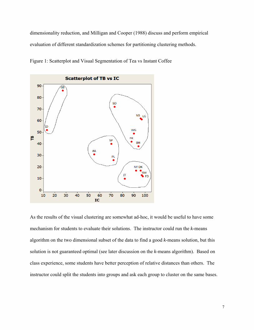
A clustering solution for k = 4 and a single combinations of breakfast food bases is given below

in Figure 1. Here, the axes units are the percentage of households which use the particular

breakfast food. All scatter plots shown is this paper were created using the “scatter plot” feature

in Minitab. However, any statistical software with a plot feature (e.g., SPSS, SAS, Excel, etc.)

could be used. It is important to ensure that the students use the same scale on both axes;

otherwise the perception of distances will not be accurate. In this example, we have not

standardized the data as all items are measured on the same scale, but for some examples

standardization or range scaling may be appropriate. For more advanced students, a discussion

of standardization, in particular the effect of standardizing the variance could be introduced. As

source materials, Naik and Kattree (1996) discuss the problems of using standardized data in

7

dimensionality reduction, and Milligan and Cooper (1988) discuss and perform empirical

evaluation of different standardization schemes for partitioning clustering methods.

Figure 1: Scatterplot and Visual Segmentation of Tea vs Instant Coffee

As the results of the visual clustering are somewhat ad-hoc, it would be useful to have some

mechanism for students to evaluate their solutions. The instructor could run the k-means

algorithm on the two dimensional subset of the data to find a good k-means solution, but this

solution is not guaranteed optimal (see later discussion on the k-means algorithm). Based on

class experience, some students have better perception of relative distances than others. The

instructor could split the students into groups and ask each group to cluster on the same bases.

8

The instructor could then evaluate the solutions by calculating both i) within cluster distances

between items and ii) the k-means criterion given in (1).

After completing several visual segmentations on combinations of two bases, the main lesson for

students is that different combinations of segmentation bases can give very different solutions.

When the exercises were given to students, students seemed to understand segmentations that

correlated to their knowledge of the world better than those that did not. For example a

segmentation with Britain and Ireland together as predominantly English speaking countries and

Spain, Portugal, and Italy together as Latin countries, seems to be sensible to the students. The

visual segmentations should be compared with one another and also should be evaluated with

respect to domain knowledge. When these exercises were tested, students were given access to a

blog/website forum (BBC 2010) that details international breakfast food information and

preferences. The students were also encouraged to view both geographical maps of Europe and

language maps of Europe in order to help put the preference information into geographical and

cultural contexts. For example, in the tea vs. coffee scatterplot, the Scandinavian countries are

grouped together, Britain and Ireland are close together, and there is a grouping of central

European countries that have high coffee consumption and moderate tea consumption. The

country clusters correspond closely to geographical distance and to language/culture. The yogurt

vs crispbread scatterplot is slightly harder to interpret. Yogurt production was first

commercialized in Western Europe in Spain (by Isaac Carasso, the founder of Danone yogurt)

and there is high yogurt consumption in Spain, Portugal, and Italy. France and the Netherlands

form a segment with high consumption of crispbread. There may be evidence of a diffusion

effect here, with yogurt having high consumption in the Mediterranean and lower consumption

where yogurt has more recently been commercialized. Overall, students with the aid of the

9

domain knowledge could find useful interpretations for some scatter plots, but not others. This

variance can be used by the instructor as i) a justification for using multiple scatter plots and ii)

as a justification for using computational techniques that use all available segmentation bases.

When comparing solutions for the same bases between groups of students, different groups may

produce slightly different segmentation solutions, which should emphasize to the students the ad-

hoc nature of visual segmentation.

As a simple exercise, the students can calculate the number of possible different scatteplots. In

the general case, there are ( )( )! ! !ndC n d n d= − possible scatterplots, where n is the number of

segmentation bases and d is the dimension of the scatter plots. In the case of this example, there

are ( )19! 2!17! 171= possible scatter plots. This exercise can be used as justification for the use

of cluster analysis and dimensionality reduction techniques. To combine the information from

171 visual segmentations would be extremely time intensive. In order to reinforce this concept,

the students could be shown/asked to create a graph of the number of features/dimensions against

the number of possible pairs of dimensions. When implementing the exercises, a dropdown

Excel formula was given to the students and the students could vary the range of dimensions and

use the Excel plotting tool to plot a graph of dimensionality against possible scatter plots.

While we used combinations of 2 segmentation bases and 2 dimensional plots, it would also be

possible use combinations of 3 segmentation bases and 3 dimensional plots. Using three

dimensional plots enables more information in each scatter plot, but perceiving distances and

drawing in clustering solutions in 3 dimensions is challenging. A possible extension exercise

would be for instructors to combine three 2 dimensional scatterplots (bases AB AC BC) into one

10

3 dimensional scatterplot (ABC) and use this as an intermediate step to the multidimensional

partitioning clustering methods introduced in section 2.3.

2.3. PARTITIONING CLUSTERING

Partitioning clustering can be introduced as a way of combining the information in all of the

segmentation bases in order to provide an aggregate segmentation. From the visual segmentation

of the 2 dimensional scatter plots, students should realize that they are trying to minimize the

distances within the clusters relative to the distances between the clusters. Given the 171 possible

visual segmentations for the 19 segmentation base breakfast cereal example, it is not hard to

press the case for a computational technique that can be used to perform segmentation across all

segmentation bases. In this example, we use k-means clustering, the partitioning algorithm most

commonly implemented in statistical software. The k-means clustering algorithm partitions a set

of items into k clusters and minimizes the total sum of differences between each item and its

cluster centroid (the average position of the items in the cluster). A review and synthesis of the

literature for the k-means technique is given by Steinley (2006). The algorithm is iterative. At

each stage of the algorithm, each item is assigned to the nearest centroid and after all

assignments have been completed, the cluster centroids are recalculated. The algorithm will

eventually converge to a stable solution. There are various ways of choosing the initial cluster

centroids. Steinley and Brusco (2007) give an overview and empirical comparison of various

initialization methods for k-means clustering. The algorithm is equivalent to minimizing the

function given in (1).

1 1min

k nj

i jj i

x c= =

−∑∑ , (1)

11

where cj is the centroid for cluster j, jix is item i in cluster j, k is the number of clusters, and n is

the number of items. The function in optimization parlance is non-convex (a locally optimal

solution may not be globally optimal) and the k-means algorithm is not guaranteed to converge

to a global optimum (Steinley, 2003). While it is not feasible to expect marketing students to

understand the technicalities of convex/non-convex optimization, it is important to emphasize

that if the algorithm is run multiple times with different starting solutions then it will possibly

give different solutions. A non-technical way of explaining this is to consider the results of the

scatter plot exercise. Different students created different clustering solutions for the same

scatterplot. While most of these solutions were good solutions, some had smaller within cluster

distances than others. Analogous to this, the k-mean algorithm has multiple attempts at finding

the solution, and the best solution can be evaluated as the one with the lowest objective score.

For k-means clustering, the number of clusters is a pre-determined input to the algorithm.

Choosing the number of clusters can be done either via i) interpretation or via ii) some set

statistical procedure. Statistical procedures, which include pseudo-F tests, information criterion

tests, and distributional tests, are summarized in Steinley (2006). However, these tests have

varying statistical assumptions and the results are often contradictory. For an applied marketing

class, it may be best to take an exploratory approach by examining and comparing interpretations

for clustering solutions across multiple values of k.

In order to bridge the gap between visual segmentation on 2 bases/dimensions and k-means

clustering on multiple dimensions the following simple exercise can be performed on a subset of

the data (less than 10 items should make the task manageable).

12

1. Have students manually plot items on a 2D scatterplot using a combination of two

segmentation bases. The students can either draw the scatterplots on Minitab/SPSS and

print them out or draw them on graph paper. The same scale must be used on both

dimensions.

2. Randomly (can use closed eyes and a pencil) select k points in the range of the scatter

plot. These points are the cluster seeds.

3. Using a ruler, assign each item to the nearest cluster seed. A ruler can be used to measure

distances.

4. Reset each cluster seed to be situated at the average coordinates of all of items assigned

to the seed (the cluster centroid).

5. Repeat steps 3 and 4 until the algorithm converges (no items are reassigned).

The exercise is a simple implementation of the k-means algorithm in 2 dimensions. The

advantage of this approach is that the instructor does not need to worry about teaching the idea of

distance metrics across multiple dimensions. The Euclidean distance can be measured with a

ruler. If the instructor wishes, the Euclidean distance across more than 2 dimensions can be

described as an extension of the “ruler” distance in 2 dimensions. As an additional step between

the visual 2 dimensional segmentations and the use of the k-means algorithm on all possible

segmentation bases, k-means can be implemented on the segmentation bases included in the 3-4

scatter plots devised by the students. This gives the students a frame of reference for the

computational segmentation. The students should realize that the k-means segmentation

combines information from the 3-4 manual segmentations.

13

2.4. MULTIDIMENSIONAL SCALING

If the computational k-means solution is considered to be an extension of visual segmentation

that uses information from all of the segmentation bases, it must be overlaid onto a visualization

that combines information from all of the segmentation bases. Such visualizations can be

created using a dimensionality reduction technique such as principal components analysis (PCA)

or multidimensional scaling (MDS). We utilize distance based MDS, which creates a lower

dimensional embedding of high dimensional data by minimizing the function given in (2).

( )2

2

ˆij ij

i j

iji j

d dStress

d

−=∑∑∑∑

(2)

Here ( )ˆij ijd F δ= is the transformed proximity between items i and j and dij is the distance

between i and j in the low dimensional space (dij). For the purpose of the exercise, the

proximities were derived using Euclidean distances from the source data. Given the metric

nature of the data, a metric ratio scale transformation was used, with a linear regression function

F. More details are given in Borg and Groenen (2005).

MDS can be explained in terms of combining the information in the 171 scatter plots. As per the

k-means clustering algorithm, the students could be asked to create MDS solutions from the

same combinations of segmentation bases contained in the 2 dimensional scatter plots as an

intermediate step between the manual scatter plots and the computational MDS solution derived

from all segmentation bases.

For the example, the MDS solution was created using the PROXSCAL procedure in SPSS,

which utilizes the SMACOF majorization method (see Borg and Groenen 2005, pp.135-157).

14

The function given in (2) is non-convex. To get around this problem, PROXSCAL allows for

multiple random starts. For the purpose of the exercise, we use 100+ random starts as

recommended by Arabie (1973).

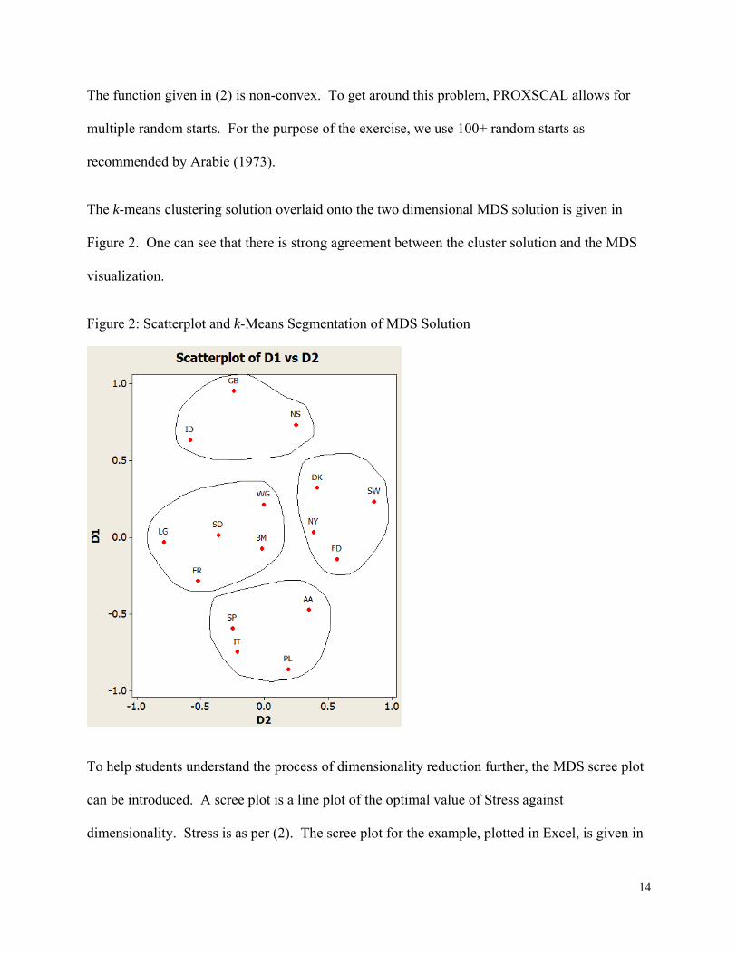
The k-means clustering solution overlaid onto the two dimensional MDS solution is given in

Figure 2. One can see that there is strong agreement between the cluster solution and the MDS

visualization.

Figure 2: Scatterplot and k-Means Segmentation of MDS Solution

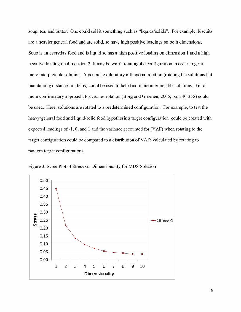
To help students understand the process of dimensionality reduction further, the MDS scree plot

can be introduced. A scree plot is a line plot of the optimal value of Stress against

dimensionality. Stress is as per (2). The scree plot for the example, plotted in Excel, is given in

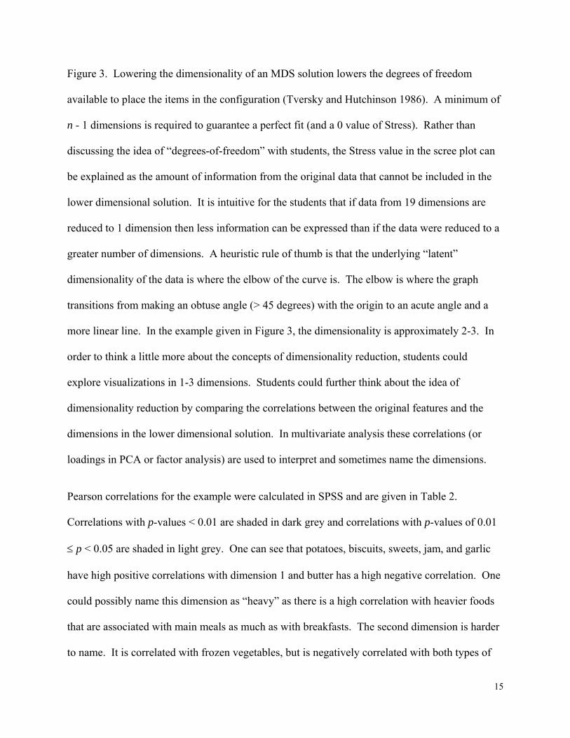
15

Figure 3. Lowering the dimensionality of an MDS solution lowers the degrees of freedom

available to place the items in the configuration (Tversky and Hutchinson 1986). A minimum of

n - 1 dimensions is required to guarantee a perfect fit (and a 0 value of Stress). Rather than

discussing the idea of “degrees-of-freedom” with students, the Stress value in the scree plot can

be explained as the amount of information from the original data that cannot be included in the

lower dimensional solution. It is intuitive for the students that if data from 19 dimensions are

reduced to 1 dimension then less information can be expressed than if the data were reduced to a

greater number of dimensions. A heuristic rule of thumb is that the underlying “latent”

dimensionality of the data is where the elbow of the curve is. The elbow is where the graph

transitions from making an obtuse angle (> 45 degrees) with the origin to an acute angle and a

more linear line. In the example given in Figure 3, the dimensionality is approximately 2-3. In

order to think a little more about the concepts of dimensionality reduction, students could

explore visualizations in 1-3 dimensions. Students could further think about the idea of

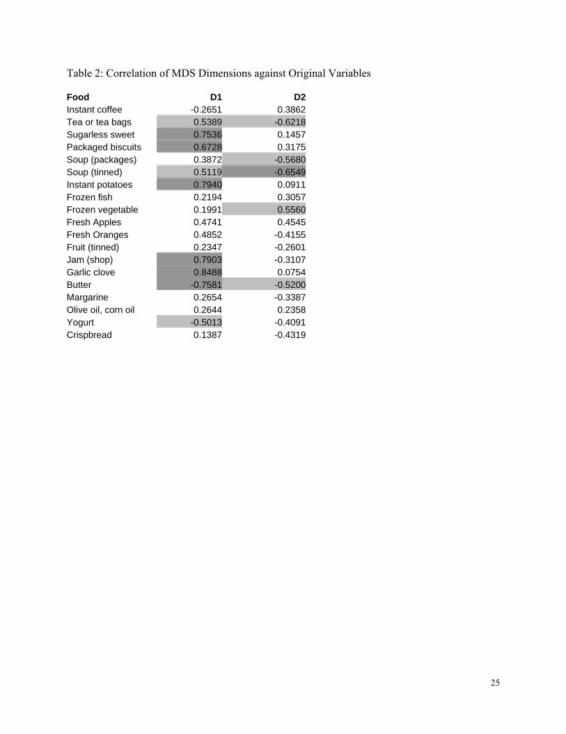
dimensionality reduction by comparing the correlations between the original features and the

dimensions in the lower dimensional solution. In multivariate analysis these correlations (or

loadings in PCA or factor analysis) are used to interpret and sometimes name the dimensions.

Pearson correlations for the example were calculated in SPSS and are given in Table 2.

Correlations with p-values < 0.01 are shaded in dark grey and correlations with p-values of 0.01

≤ p < 0.05 are shaded in light grey. One can see that potatoes, biscuits, sweets, jam, and garlic

have high positive correlations with dimension 1 and butter has a high negative correlation. One

could possibly name this dimension as “heavy” as there is a high correlation with heavier foods

that are associated with main meals as much as with breakfasts. The second dimension is harder

to name. It is correlated with frozen vegetables, but is negatively correlated with both types of

16

soup, tea, and butter. One could call it something such as “liquids/solids”. For example, biscuits

are a heavier general food and are solid, so have high positive loadings on both dimensions.

Soup is an everyday food and is liquid so has a high positive loading on dimension 1 and a high

negative loading on dimension 2. It may be worth rotating the configuration in order to get a

more interpretable solution. A general exploratory orthogonal rotation (rotating the solutions but

maintaining distances in items) could be used to help find more interpretable solutions. For a

more confirmatory approach, Procrustes rotation (Borg and Groenen, 2005, pp. 340-355) could

be used. Here, solutions are rotated to a predetermined configuration. For example, to test the

heavy/general food and liquid/solid food hypothesis a target configuration could be created with

expected loadings of -1, 0, and 1 and the variance accounted for (VAF) when rotating to the

target configuration could be compared to a distribution of VAFs calculated by rotating to

random target configurations.

Figure 3: Scree Plot of Stress vs. Dimensionality for MDS Solution

0.00

0.05

0.10

0.15

0.20

0.25

0.30

0.35

0.40

0.45

0.50

1 2 3 4 5 6 7 8 9 10

Dimensionality

Stre

ss

Stress-1

17

---------------------------------------------------------------------------------------------------------------------

INSERT Table 2 Here

---------------------------------------------------------------------------------------------------------------------

2.5. HIERARCHICAL CLUSTERING

As a final exercise, the students are asked to produce a hierarchical clustering solution. This is

done in order to give the students an additional perspective on how data can be structured and

interpreted. Hierarchical clustering can be introduced as a technique for giving an overall picture

of linkages between items. Hierarchical clustering techniques can be split into two major

subgroups, agglomerative clustering techniques and divisive clustering techniques. We

concentrate on agglomerative techniques as these techniques are more widely implemented in

statistical packages. In agglomerative clustering, each object starts off as an individual cluster

and then at each iteration of the algorithm two clusters are combined. The algorithm terminates

when only a single cluster remains. The algorithm can be explored by students in two

dimensions in a similar fashion to the example described for k-means clustering. Given that n ×

(n – 1) / 2 distances need to be calculated, it may only be feasible to use a small subset of the

data.

1. Give the students some graph paper and have them manually plot items on a 2

dimensional scatterplot using a combination of two segmentation bases. The same scale

must be used on both dimensions. Number each item as an individual cluster.

2. Calculate Euclidean distances between each pair of clusters. This can be done using a

ruler.

18

3. Merge the two clusters with the smallest distance between the clusters. Give the

combined cluster a new number and rename the merged cluster. E.g., For the 1st iteration

of a 8 item problem, where clusters 2 and 4 are merged, record {2,4}→{9}.

4. Calculate the distance between the merged cluster and every other cluster (excluding the

component clusters of the merged cluster). This can be done in several ways. In single

linkage clustering the minimum distance between items in the clusters is used, in

complete linkage clustering the maximum distance is used, and in average linkage

clustering the average distance is used. A description of 5 methods of calculating

distances for hierarchical clustering and of some of the properties of solutions created by

these methods is given in Lattin, Carroll, and Green (2002), pp. 280-288. For example,

given two clusters A and B to be merged, the distance between the combined cluster and

another cluster C is ( ) ( ){ }min , , ,dist a c dist a b for single linkage clustering,

( ) ( ){ }max , , ,dist a c dist a b for complete linkage clustering, and

( ) ( )1 2

1 2

, ,n dist a c n dist a bn n++

for average linkage clustering, where n1 is the number of items

in cluster 1, n2 is the number of items in cluster 2, and a, b, and c are items in the clusters

A, B, and C respectively.

5. Repeat steps 3-4 until all items are in a single cluster.

The exercise can also be completed using distances across all segmentation bases, but as per the

k-means clustering exercise, the instructor may wish to avoid the discussion of distance metrics

on multidimensional data. The manual calculation of agglomerative hierarchical clustering

methods is very time intensive, so an instructor may quickly wish to move on to the use of

19

computational packages. Most statistical software packages offer a range of hierarchical

clustering techniques, including the three methods mentioned previously, centroid clustering,

Ward’s method, and density linkage clustering. Ward’s method aims to minimize within cluster

variance and is the close analogue of k-means clustering. Students should be encouraged to

experiment with the different hierarchical clustering functions. The preferred type of clustering

to be used may depend on the application. For example, single-linkage clustering tends to

produce long thin “chained” clusters, while complete linkage clustering tends to produce more

circular clusters.

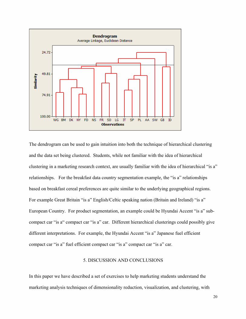
A dendrogram gives a pictorial representation of the hierarchical classification tree. The heights

of the tree (cluster joins) are the distances between the clusters to be joined. These distances

conform to the ultrametric inequality. The distance properties of hierarchical clustering are

probably beyond the scope of an undergraduate or MBA marketing research class. A discussion

and some proofs of these properties are given in Milligan (1979). A dendrogram for the

breakfast foods example, created in SPSS, is given in Figure 4. The hierarchy was created using

average linkage clustering. In order to get the students to consider the relationship between

hierarchical clustering and partitioning clustering the students could be asked to take a cut of the

hierarchical solution for a given value of k. An example for k = 4 is given in Figure 4. There are

four clusters at the level of the cut.

Figure 4: Hierarchical Clustering Dendrogram with Cut at k = 4

20

The dendrogram can be used to gain intuition into both the technique of hierarchical clustering

and the data set being clustered. Students, while not familiar with the idea of hierarchical

clustering in a marketing research context, are usually familiar with the idea of hierarchical “is a”

relationships. For the breakfast data country segmentation example, the “is a” relationships

based on breakfast cereal preferences are quite similar to the underlying geographical regions.

For example Great Britain “is a” English/Celtic speaking nation (Britain and Ireland) “is a”

European Country. For product segmentation, an example could be Hyundai Accent “is a” sub-

compact car “is a“ compact car “is a” car. Different hierarchical clusterings could possibly give

different interpretations. For example, the Hyundai Accent “is a” Japanese fuel efficient

compact car “is a” fuel efficient compact car “is a” compact car “is a” car.

5. DISCUSSION AND CONCLUSIONS

In this paper we have described a set of exercises to help marketing students understand the

marketing analysis techniques of dimensionality reduction, visualization, and clustering, with

21

particular application to market segmentation. These techniques are usually taught in the last

couple of classes in an undergraduate marketing research course. These techniques are often

taught using a black box approach, with students analyzing data using these techniques but

having little understanding of how the techniques work. The exercises described in this paper

start by having the students visually implement these techniques using sets of 2 dimensional

data. The techniques are then implemented computationally using multidimensional data. The

emphasis is on showing linkages between the techniques and on justifying the multidimensional

techniques as necessary due to the impracticality of visual segmentation as dimensionality

increases.

The exercises were developed and tested in both undergraduate marketing research and

international marketing classes. The classes were held in two different universities. Both these

universities are categorized as “urban research universities” and serve diverse student

populations including many first generation college students. The classes received positive

feedback and it was gratifying that the students used the techniques in their group projects. The

group projects entailed the analysis of a real world business problem. For the international

marketing class, the students had to justify and plan the market entry of a new product into a

target market. The students used the techniques described in the exercises to help

parsimoniously represent multidimensional data and to help justify the choice of country of

entry.

22

6. REFERENCES

Arabie, P. (1973), "Concerning Monte Carlo Evaluations of Nonmetric Multidimensional

Scaling Algorithms," Psychometrika, 38, 607-608.

Arabie, P., Carroll, J. D., DeSarbo, W. S., Wind, J. (1981), "Overlapping Clustering: A New

Method for Product Positioning," Journal of Marketing Research, 18, 310-317.

BBC (2010), “Great International Breakfast Dishes,” http://www.bbc.co.uk/dna/h2g2/A930197.

Borg, I. and Groenen, P. J. F. (2005), Modern Multidimensional Scaling: Theory and

Applications, New York, NY: Springer.

Elrod, T. (1988), “Choice Map: Inferring a Product-Market Map from Panel Data,” Marketing

Science, 7, 21-40.

Hauser, J. R. and Simmie, P. (1981), "Profit Maximizing Perceptual Positions: An Integrated

Theory for the Selection of Product Features and Price," Management Science, 27, 33-56.

Kotabe, M. and Helsen, K. (2010), Global Marketing Management, Hoboken, NJ: Wiley.

Lattin, J., Carroll, J. D. and Green, P. E. (2002), Analyzing Multivariate Data, Pacific Grove,

CA: Duxbury Press.

Love, T. E. and Hildebrand, D. K. (2002), "Statistics Education and the Making Statistics More

Effective in Schools of Business," The American Statistician, 56, 107-112.

Milligan, G. W. (1979), “Ultrametric Hierarchical Clustering Algorithms,” Psychometrika, 44,

343-346.

23

Milligan, G. W. and Cooper, M. C. (1988), "A Study of Standardization of Variables in Cluster

Analysis," Journal of Classification, 5, 181-204.

Naik, D. N. and Khattree, R. (1996), "Revisiting Olympic Track Records: Some Practical

Considerations in the Principal Component Analysis," The American Statistician, 50, 140-144.

Parasuraman, A., Grewel, D. and Krishnan, R. (2007), Marketing Research, Boston MA:

Houghton Mifflin

Peterson, M. Malhotra, N. (2000), "Country Segmentation based on Objective Quality-of-Life

Measures," International Marketing Review, 17, 56-73.

Steinley, D. (2003), "Local Optima in k-Means Clustering: What You Don’t Know May Hurt

You," Psychological Methods, 8, 294-304.

Steinley, D. (2006), "k-Means clustering: A half-century synthesis,"British Journal of

Mathematical and Statistical Psychology, 59, 1-34.

Steinley, D. and Brusco, M. J. (2007), "Initializing k-Means Batch Clustering: A Critical

Evaluation of Several Techniques," Journal of Classification, 24, 99-121.

Tversky, A. and Hutchinson, J. W. (1986), "Nearest Neighbor Analysis of Psychological

Spaces," Psychological Review, 93, 3-22.

Vyncke, P. (2002), “Lifestyle Segmentation: From Attitudes, Interests and Opinions, to Values,

Aesthetic Styles, Life Visions and Media Preferences,” European Journal of Communication,

17, 445-463

24

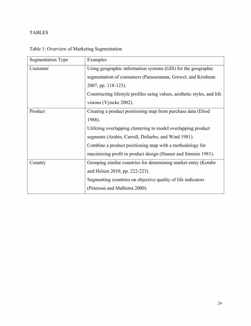
TABLES

Table 1: Overview of Marketing Segmentation

Segmentation Type Examples

Customer Using geographic information systems (GIS) for the geographic

segmentation of consumers (Parasuraman, Grewel, and Krishnan

2007, pp. 118-123).

Constructing lifestyle profiles using values, aesthetic styles, and life

visions (Vyncke 2002).

Product Creating a product positioning map from purchase data (Elrod

1988).

Utilizing overlapping clustering to model overlapping product

segments (Arabie, Carroll, DeSarbo, and Wind 1981).

Combine a product positioning map with a methodology for

maximizing profit in product design (Hauser and Simmie 1981).

Country Grouping similar countries for determining market entry (Kotabe

and Helsen 2010, pp. 222-223).

Segmenting countries on objective quality of life indicators

(Peterson and Malhotra 2000).

25

Table 2: Correlation of MDS Dimensions against Original Variables

Food D1 D2Instant coffee -0.2651 0.3862Tea or tea bags 0.5389 -0.6218Sugarless sweet 0.7536 0.1457Packaged biscuits 0.6728 0.3175Soup (packages) 0.3872 -0.5680Soup (tinned) 0.5119 -0.6549Instant potatoes 0.7940 0.0911Frozen fish 0.2194 0.3057Frozen vegetable 0.1991 0.5560Fresh Apples 0.4741 0.4545Fresh Oranges 0.4852 -0.4155Fruit (tinned) 0.2347 -0.2601Jam (shop) 0.7903 -0.3107Garlic clove 0.8488 0.0754Butter -0.7581 -0.5200Margarine 0.2654 -0.3387Olive oil, corn oil 0.2644 0.2358Yogurt -0.5013 -0.4091Crispbread 0.1387 -0.4319