Embed Size (px)
Citation preview
Speech and Language Processing: An introduction to natural language processing,computational linguistics, and speech recognition. Daniel Jurafsky & James H.Martin. Copyright c© 2006, All rights reserved. Draft of August 3, 2006. Donot cite without permission.
24 MACHINE TRANSLATION
The process of translating comprises in its essence the whole secret ofhuman understanding and social communication.
Attributed to Hans-Georg Gadamer
This chapter introduces techniques formachine translation (MT ), the useMACHINETRANSLATION
MT of computers to automate some or all of the process of translating from one lan-guage to another. Translation, in its full generality, is a difficult, fascinating, andintensely human endeavor, as rich as any other area of human creativity. Considerthe following passage from the end of Chapter 45 of the 18th-century novelTheStory of the Stone, also calledDream of the Red Chamber, by Cao Xue Qin (Cao,1792), transcribed in the Mandarin dialect:
dai yu zi zai chuang shang gan nian bao chai. . . you ting jian chuang wai zhu shaoxiang ye zhe shang, yu sheng xi li, qing han tou mu, bu jue you dixia lei lai.
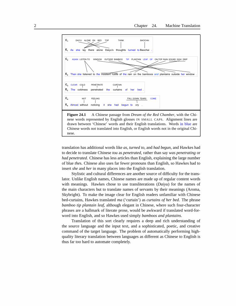
Fig. 24.1 shows the English translation of this passage by David Hawkes, insentences labeled E1-E4. For ease of reading, instead of giving the Chinese, wehave shown the English glosses of each Chinese wordIN SMALL CAPS. Wordsin blueare Chinese words not translated into English, or English words not in theChinese. We have shownalignment lines between words that roughly correspondin the two languages.
Consider some of the issues involved in this translation. First, the Englishand Chinese texts are very different structurally and lexically. The four Englishsentences (notice the periods in blue) correspond to one long Chinese sentence.The word order of the two texts is very different, as we can seeby the many crossedalignment lines in Fig. 24.1. The English has many more wordsthan the Chinese,as we can see by the large number of English words marked in blue. Many ofthese differences are caused by structural differences between the two languages.For example, because Chinese rarely marks verbal aspect or tense; the English
2 Chapter 24. Machine Translation
Figure 24.1 A Chinese passage fromDream of the Red Chamber, with the Chi-nese words represented by English glossesIN SMALL CAPS. Alignment lines aredrawn between ‘Chinese’ words and their English translations. Wordsin blue areChinese words not translated into English, or English wordsnot in the original Chi-nese.
translation has additional words likeas, turned to, andhad begun, and Hawkes hadto decide to translate Chinesetouaspenetrated, rather than saywas penetratingorhad penetrated. Chinese has less articles than English, explaining the large numberof blue thes. Chinese also uses far fewer pronouns than English, so Hawkes had toinsertsheandher in many places into the English translation.
Stylistic and cultural differences are another source of difficulty for the trans-lator. Unlike English names, Chinese names are made up of regular content wordswith meanings. Hawkes chose to use transliterations (Daiyu) for the names ofthe main characters but to translate names of servants by their meanings (Aroma,Skybright). To make the image clear for English readers unfamiliar with Chinesebed-curtains, Hawkes translatedma (‘curtain’) ascurtains of her bed. The phrasebamboo tip plantain leaf, although elegant in Chinese, where such four-characterphrases are a hallmark of literate prose, would be awkward iftranslated word-for-word into English, and so Hawkes used simplybamboos and plantains.
Translation of this sort clearly requires a deep and rich understanding ofthe source language and the input text, and a sophisticated,poetic, and creativecommand of the target language. The problem of automatically performing high-quality literary translation between languages as different as Chinese to English isthus far too hard to automate completely.

3
However, even non-literary translations between such similar languages asEnglish and French can be difficult. Here is an English sentence from the Hansardscorpus of Canadian parliamentary proceedings, with its French translation:
English: Following a two-year transitional period, the new Foodstuffs Ordinancefor Mineral Water came into effect on April 1, 1988. Specifically, it contains morestringent requirements regarding quality consistency andpurity guarantees.French: La nouvelle ordonnance federale sur les denrees alimentaires concernantentre autres les eaux minerales, entree en vigueur le ler avril 1988 apres une periodetransitoire de deux ans. exige surtout une plus grande constance dans la qualite etune garantie de la purete.French gloss:THE NEW ORDINANCE FEDERAL ON THE STUFF FOOD CONCERN-ING AMONG OTHERS THE WATERS MINERAL CAME INTO EFFECT THE1ST APRIL
1988 AFTER A PERIOD TRANSITORY OF TWO YEARS REQUIRES ABOVE ALL A
LARGER CONSISTENCY IN THE QUALITY AND A GUARANTEE OF THE PURITY.
Despite the strong structural and vocabulary overlaps between English andFrench, such translation, like literary translation, still has to deal with differencesin word order (e.g., the location of thefollowing a two-year transitional periodphrase) and in structure (e.g., English uses the nounrequirementswhile the Frenchuses the verbexige‘ REQUIRE’).
Nonetheless, such translations are much easier, and a number of non-literarytranslation tasks can be addressed with current computational models of machinetranslation, including: (1) tasks for which arough translation is adequate, (2)tasks where a humanpost-editor is used, and (3) tasks limited to smallsublan-guagedomains in whichfully automatic high quality translation (FAHQT) isFULLY AUTOMATIC
HIGH QUALITYTRANSLATION
still achievable.Information acquisition on the web is the kind of task where arough trans-
lation may still be useful. Suppose you were at the market this morning and sawsome lovelyplatanos(plantains, a kind of banana) at the local Caribbean grocerystore and you want to know how to cook them. You go to the web, and find thefollowing recipe:
Platano en Naranja Para 6 personas3 Platanos maduro 2 cucharadas de mantequilla derretida1 taza de jugo (zumo) de naranja 5 cucharadas de azucar morena o blanc1/8 cucharadita de nuez moscada en polvo 1 cucharada de ralladura de naranja1 cucharada de canela en polvo (opcional)
Pelar los platanos, cortarlos por la mitad y, luego, a lo largo. Engrasaruna fuente opirex con margarina. Colocar los platanos y banarlos con la mantequilla derretida. En unrecipiente hondo, mezclar el jugo (zumo) de naranja con el azucar, jengibre, nuez moscaday ralladura de naranja. Verter sobre los platanos y hornear a 325◦ F. Los primeros 15minutos, dejar los patanos cubiertos, hornear 10 o 15 minutos mas destapando los pltanos

4 Chapter 24. Machine Translation
An MT engine produces the following translation:
Banana in Orange For 6 people3 mature Bananas 2 spoonfuls of mantequilla melted1 cup of juice (juice) of orange 5 spoonfuls of brown or white sugar1/8 teaspoon of nut moscada in dust 1 spoonful of ralladura oforange1 spoonful of dust cinnamon (optional)
Pelar the bananas, to cut them by half and, soon, along. To lubricate a source or pirexwith margarina. To place bananas and to bathe them with mantequilla melted. In a deepcontainer, to mix the juice (juice) of orange with the sugar,jengibre, moscada nut andralladura of orange. To spill on 325 bananas and to hornear to◦ F. The first 15 minutes,to leave bananas covered, to hornear 10 or 15 minutes more opening bananas.
While there are still lots of confusions in this translation(is it for bananasor plantains? What exactly is the pot we should use? What aremantequillaandralladura?) it’s probably enough, perhaps after looking up one or two words, toget a basic idea of something to try in the kitchen with your new purchase!
An MT system can also be used to speed-up the human translation process,by producing a draft translation that is fixed up in apost-editingphase by a humanPOSTEDITING
translator. Strictly speaking, systems used in this way aredoingcomputer-aidedhuman translation (CAHT or CAT) rather than (fully automatic) machine trans-COMPUTERAIDED
HUMANTRANSLATION
lation. This model of MT usage is effective especially for high volume jobs andthose requiring quick turn-around, such as the translationof software manuals forlocalization to reach new markets.LOCALIZATION
Weather forecasting is an example of asublanguagedomain that can be mod-SUBLANGUAGE
eled completely enough to use raw MT output even without post-editing. Weatherforecasts consist of phrases likeCloudy with a chance of showers today and Thurs-day, or Outlook for Friday: Sunny. This domain has a limited vocabulary andonly a few basic phrase types. Ambiguity is rare, and the senses of ambiguouswords are easily disambiguated based on local context, using word classes and se-mantic features such asWEEKDAY, PLACE, or TIME POINT. Other domains thatare sublanguage-like include equipment maintenance manuals, air travel queries,appointment scheduling, and restaurant recommendations.
Applications for machine translation can also be characterized by the numberand direction of the translations. Localization tasks liketranslations of computermanuals require one-to-many translation (from English into many languages). One-to-many translation is also needed for non-English speakers around the world toaccess web information in English. Conversely, many-to-one translation (into En-glish) is relevant for anglophone readers who need the gist of web content writtenin other languages. Many-to-many translation is relevant for environments like theEuropean Union, where eleven official languages need to be intertranslated.

Section 24.1. Why is Machine Translation So Hard? 5
Before we turn to MT systems, we begin in section 24.1 by summarizing keydifferences among languages. The three classic models for doing MT are then pre-sented in Sec. 24.2: thedirect, transfer, andinterlingua approaches. We then in-vestigate in detail modernstatistical MT in Secs. 24.3-24.8, finishing in Sec. 24.9with a discussion ofevaluation.
24.1 WHY IS MACHINE TRANSLATION SO HARD?
We began this chapter with some of the issues that made it hardto translateTheStory of the Stonefrom Chinese to English. In this section we look in more detailabout what makes translation difficult. We’ll discuss what makes languages similaror different, includingsystematicdifferences that we can model in a general way,as well asidiosyncratic and lexical differences that must be dealt with one by one.
24.1.1 Typology
When you accidentally pick up a radio program in some foreignlanguage it seemslike chaos, completely unlike the familiar languages of your everyday life. Butthere are patterns in this chaos, and indeed, some aspects ofhuman language seemto beuniversal, holding true for every language. Many universals arise from theUNIVERSAL
functional role of language as a communicative system by humans. Every lan-guage, for example, seems to have words for referring to people, for talking aboutwomen, men, and children, eating and drinking, for being polite or not. Other uni-versals are more subtle; for example Ch. 5 mentioned that every language seems tohave nouns and verbs.
Even when languages differ, these differences often have systematic struc-ture. The study of systematic cross-linguistic similarities and differences is calledtypology (Croft (1990), Comrie (1989)). This section sketches some typologicalTYPOLOGY
facts about crosslinguistic similarity and difference.Morphologically , languages are often characterized along two dimensions
of variation. The first is the number of morphemes per word, ranging from iso-lating languages like Vietnamese and Cantonese, in which each wordgenerallyISOLATING
has one morpheme, topolysynthetic languages like Siberian Yupik (“Eskimo”), inPOLYSYNTHETIC
which a single word may have very many morphemes, corresponding to a wholesentence in English. The second dimension is the degree to which morphemesare segmentable, ranging fromagglutinative languages like Turkish (discussed inAGGLUTINATIVE
Ch. 3), in which morphemes have relatively clean boundaries, to fusion languagesFUSION
like Russian, in which a single affix may conflate multiple morphemes, like-om inthe wordstolom, (table-SG-INSTR-DECL1) which fuses the distinct morphological

6 Chapter 24. Machine Translation
categories instrumental, singular, and first declension.Syntactically, languages are perhaps most saliently different in the basic
word order of verbs, subjects, and objects in simple declarative clauses. German,French, English, and Mandarin, for example, are allSVO (Subject-Verb-Object)SVO
languages, meaning that the verb tends to come between the subject and object.Hindi and Japanese, by contrast, areSOV languages, meaning that the verb tendsSOV
to come at the end of basic clauses, while Irish, Arabic, and Biblical Hebrew areVSO languages. Two languages that share their basic word-ordertype often haveVSO
other similarities. For exampleSVO languages generally haveprepositionswhileSOV languages generally havepostpositions.
For example in the following SVO English sentence, the verbadoresis fol-lowed by its argument VPlistening to music, the verblistening is followed byits argument PPto music, and the prepositionto is followed by its argumentmu-sic. By contrast, in the Japanese example which follows, each ofthese orderingsis reversed; both verbsprecedetheir arguments, and the postposition follows itsargument.
(24.1) English: He adores listening to musicJapanese:kare
heha ongaku
musicwoto
kikulistening
no ga daisukiadores
desu
Another important dimension of typological variation has to do with argu-ment structure andlinking of predicates with their arguments, such as the differ-ence betweenhead-marking anddependent-markinglanguages (Nichols, 1986).HEADMARKING
Head-marking languages tend to mark the relation between the head and its depen-dents on the head. Dependent-marking languages tend to markthe relation on thenon-head. Hungarian, for example, marks the possessive relation with an affix (A)on the head noun (H), where English marks it on the (non-head)possessor:
(24.2) English:Hungarian:
theazthe
man-A’semberman
HhouseHhaz-Aahouse-his
Typological variation in linking can also relate to how the conceptual propertiesof an event are mapped onto specific words. Talmy (1985) and (1991) noted thatlanguages can be characterized by whether direction of motion and manner of mo-tion are marked on the verb or on the “satellites”: particles, prepositional phrases,or adverbial phrases. For example a bottle floating out of a cave would be de-scribed in English with the direction marked on the particleout, while in Spanishthe direction would be marked on the verb:
(24.3) English: The bottle floated out.Spanish: La
Thebotellabottle
salioexited
flotando.floating.

Section 24.1. Why is Machine Translation So Hard? 7
Verb-framed languages mark the direction of motion on the verb (leavingVERBFRAMED
the satellites to mark the manner of motion), like Spanishacercarse‘approach’,alcanzar‘reach’, entrar ‘enter’, salir ‘exit’ Satellite-framed languages mark theSATELLITEFRAMED
direction of motion on the satellite (leaving the verb to mark the manner of motion),like Englishcrawl out, float off, jump down, walk over to, run after. Languages likeJapanese, Tamil, and the many languages in the Romance, Semitic, and Mayan lan-guages families, are verb-framed; Chinese as well as non-Romance Indo-Europeanlanguages like English, Swedish, Russian, Hindi, and Farsi, are satellite-framed(Talmy, 1991; Slobin, 1996).
Finally, languages vary along a typological dimension related to the thingsthey can omit. Many languages require that we use an explicitpronoun when talk-ing about a referent that is given in the discourse. In other languages, however, wecan sometimes omit pronouns altogether as the following examples from Spanishand Chinese show, using the/0-notation introduced in Ch. 20:
(24.4) [El jefe]i dio con un libro./0i Mostro a un descifrador ambulante.[The boss]came upon a book.[He] showed it to a wandering decoder.
(24.5) CHINESE EXAMPLE
Languages which can omit pronouns in these ways are calledpro-drop lan-PRODROP
guages. Even among the pro-drop languages, their are markeddifferences frequen-cies of omission. Japanese and Chinese, for example, tend toomit far more thanSpanish. We refer to this dimension asreferential density; languages which tendREFERENTIAL
DENSITY
to use more pronouns are more referentially dense than thosethat use more zeros.Referentially sparse languages, like Chinese or Japanese,that require the hearer todo more inferential work to recover antecedents are calledcold languages. Lan-COLD
guages that are more explicit and make it easier for the hearer are calledhot lan-HOT
guages.1 (Bickel, 2003)Each typological dimension can cause problems when translating between
languages that differ along them. Obviously translating from SVO languages likeEnglish to SOV languages like Japanese requires huge structural reorderings, sinceall the constituents are at different places in the sentence. Translating from asatellite-framed to a verb-framed language, or from a head-marking to a dependent-marking language, requires changes to sentence structure and constraints on wordchoice. Languages with extensive pro-drop, like Chinese orJapanese, cause hugeproblems for translation into non-pro-drop languages likeEnglish, since each zerohas to be identified and the anaphor recovered.
1 The termshot andcold are borrowed from Marshall McLuhan’s (1964) distinction between hotmedia like movies, which fill in my details for the viewer, versus cold media like comics, whichrequire the reader to do more inferential work to fill out the representation.

8 Chapter 24. Machine Translation
24.1.2 Other Structural Divergences
Many structural divergences between languages are based ontypological differ-ences. Others, however, are simply idiosyncratic differences that are characteristicof particular languages or language pairs. For example in English the unmarkedorder in a noun-phrase has adjectives precede nouns, but in French and Spanishadjectives generally follow nouns.2
(24.6)Spanish bruja verde French maison bleu
witch green house blueEnglish “green witch” “blue house”
Chinese relative clauses are structured very differently than English relativeclauses, making translation of long Chinese sentences verycomplex.
Language-specific constructions abound. English, for example, has an id-iosyncratic syntactic construction involving the wordthere that is often used tointroduce a new scene in a story, as inthere burst into the room three men withguns. To give an idea of how trivial, yet crucial, these differences can be, think ofdates. Dates not only appear in various formats — typically DD/MM/YY in BritishEnglish, MM/DD/YY in American English, and YYMMDD in Japanese—but thecalendars themselves may also differ. Dates in Japanese, for example, are oftenrelative to the start of the current Emperor’s reign rather than to the start of theChristian Era.
24.1.3 Lexical Divergences
Lexical divergences also cause huge difficulties in translation. We saw in Ch. 19,for example, that the English source language wordbasscould appear in Spanishas the fishlubinaor the instrumentbajo. Thus translation often requires solving theexact same problems as word sense disambiguation, and the two fields are closelylinked.
In English the wordbassis homonymous; the two senses of the word are notclosely related semantically, and so it is natural that we would have to disambiguatein order to translate. Even in cases of polysemy, however, weoften have to disam-biguate if the target language doesn’t have the exact same kind of polysemy. TheEnglish wordknow, for example, is polysemous; it can refer to knowing of a factor proposition (I know that snow is white) or familiarity with a person or location (Iknow Jon Stewart. It turns out that translating these different senses requires usingdistinct French verbs, including the verbsconnaıtre, andsavoir. Savoiris generally
2 As always, there are exceptions to this generalization, such asgalore in English andgros inFrench; furthermore in French some adjectives can appear before the noun with a different meaning;route mauvaise‘bad road, badly-paved road’ versusmauvaise route‘wrong road’ (Waugh, 1976).
Section 24.1. Why is Machine Translation So Hard? 9
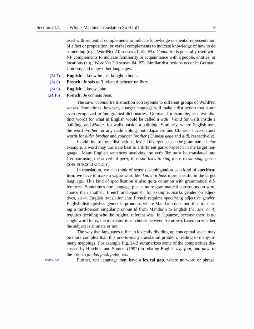
used with sentential complements to indicate knowledge or mental representationof a fact or proposition, or verbal complements to indicate knowledge of how to dosomething (e.g., WordNet 2.0 senses #1, #2, #3).Connaıtre is generally used withNP complements to indicate familiarity or acquaintance with a people, entities, orlocations (e.g., WordNet 2.0 senses #4, #7). Similar distinctions occur in German,Chinese, and many other languages:
(24.7) English: I know he just bought a book.(24.8) French: Je sais qu’il vient d’acheter un livre.
(24.9) English: I know John.(24.10) French: Je connais Jean.
Thesavoir/connaıtre distinction corresponds to different groups of WordNetsenses. Sometimes, however, a target language will make a distinction that is noteven recognized in fine-grained dictionaries. German, for example, uses two dis-tinct words for what in English would be called awall: Wandfor walls inside abuilding, andMauer, for walls outside a building. Similarly, where English usesthe wordbrother for any male sibling, both Japanese and Chinese, have distinctwords forolder brotherandyounger brother(Chinesegegeanddidi, respectively).
In addition to these distinctions, lexical divergences canbe grammatical. Forexample, a word may translate best to a different part-of-speech in the target lan-guage. Many English sentences involving the verblike must be translated intoGerman using the adverbialgern; thus she likes to singmaps tosie singt gerne(SHE SINGS LIKINGLY).
In translation, we can think of sense disambiguation as a kind of specifica-tion; we have to make a vague word likeknowor bassmore specific in the targetlanguage. This kind of specification is also quite common with grammatical dif-ferences. Sometimes one language places more grammatical constraints on wordchoice than another. French and Spanish, for example, marksgender on adjec-tives, so an English translation into French requires specifying adjective gender.English distinguishes gender in pronouns where Mandarin does not; thus translat-ing a third-person singular pronounta from Mandarin to English (he, she, or it)requires deciding who the original referent was. In Japanese, because there is nosingle word foris, the translator must choose betweeniru or aru, based on whetherthe subject is animate or not.
The way that languages differ in lexically dividing up conceptual space maybe more complex than this one-to-many translation problem,leading to many-to-many mappings. For example Fig. 24.2 summarizes some of the complexities dis-cussed by Hutchins and Somers (1992) in relating Englishleg, foot, andpaw, tothe Frenchjambe, pied, patte, etc.
Further, one language may have alexical gap, where no word or phrase,LEXICAL GAP

10 Chapter 24. Machine Translation
Figure 24.2 The complex overlap between Englishleg, foot, etc, and variousFrench translations likepattediscussed by Hutchins and Somers (1992) .
short of an explanatory footnote, can express the meaning ofa word in the otherlanguage. For example, Japanese does not have a word forprivacy, and Englishdoes not have a word for Japaneseoyakokoor Chinesexiao (we make do with theawkward phrasefilial piety for both).
24.2 CLASSICAL MT & THE VAUQUOIS TRIANGLE
The next few sections introduce the classical pre-statistical architectures for ma-chine translation. Real systems tend to involve combinations of elements fromthese three architectures; thus each is best thought of as a point in an algorithmicdesign space rather than as an actual algorithm.
In direct translation, we proceed word-by-word through the source languagetext, translating each word as we go. Direct translation uses a large bilingual dic-tionary, each of whose entries is a small program with the jobof translating oneword. In transfer approaches, we first parse the input text, and then apply rulesto transform the source language parse structure into a target language parse struc-ture. We then generate the target language sentence from theparse structure. Ininterlingua approaches, we analyze the source language text into some abstractmeaning representation, called aninterlingua . We then generate into the targetlanguage from this interlingual representation.
A common way to visualize these three approaches is withVauquois tri-angle shown in Fig. 24.3. The triangle shows the increasing depth of analysisVAUQUOIS TRIANGLE
required (on both the analysis and generation end) as we movefrom the directapproach through transfer approaches, to interlingual approaches. In addition, itshows the decreasing amount of transfer knowledge needed aswe move up the tri-angle, from huge amounts of transfer at the direct level (almost all knowledge is

Section 24.2. Classical MT & the Vauquois Triangle 11
transfer knowledge for each word) through transfer (transfer rules only for parsetrees or thematic roles) through interlingua (no specific transfer knowledge).
Figure 24.3 The Vauquois triangle.
In the next sections we’ll see how these algorithms address some of the fourtranslation examples shown in Fig. 24.4
English Mary didn’t slap the green witch
⇒ Spanish MariaMary
nonot
diogave
unaa
bofetadaslap
ato
lathe
brujawitch
verdegreen
English The green witch is at home this week
⇒ German Diesethis
Wocheweek
istis
diethe
grunegreen
Hexewitch
zuat
Hause.house
English He adores listening to music
⇒ Japanese karehe
ha ongakumusic
woto
kikulistening
no ga daisukiadores
desu
Chinese cheng longJackie Chan
daoto
xiang gangHong Kong
qugo
⇒ English Jackie Chan went to Hong Kong
Figure 24.4 Example sentences used throughout the chapter.
24.2.1 Direct Translation
In direct translation , we proceed word-by-word through the source language text,DIRECTTRANSLATION
12 Chapter 24. Machine Translation
translating each word as we go. We make use of no intermediatestructures, ex-cept for shallow morphological analysis; each source word is directly mapped ontosome target word. Direct translation is thus based on a largebilingual dictionary;each entry in the dictionary can be viewed as a small program whose job is to trans-late one word. After the words are translated, simple reordering rules can apply,for example for moving adjectives after nouns when translating from English toFrench.
The guiding intuition of the direct approach is that we translate by incremen-tally transforming the source language text into a target language text. While thepure direct approach is no longer used, this transformational intuition underliesboth modern commercial systems like Systran and modern research systems basedon statistical MT.
Figure 24.5 Direct machine translation. The major component, indicated by sizehere, is the bilingual dictionary.
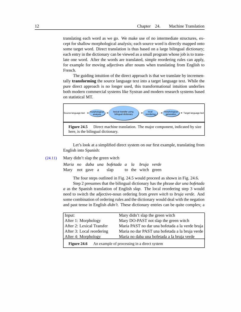
Let’s look at a simplified direct system on our first example, translating fromEnglish into Spanish:
(24.11) Mary didn’t slap the green witch
MariaMary
nonot
dabagave
unaa
bofetadaslap
ato
lathe
brujawitch
verdegreen
The four steps outlined in Fig. 24.5 would proceed as shown inFig. 24.6.Step 2 presumes that the bilingual dictionary has the phrasedar una bofetada
a as the Spanish translation of Englishslap. The local reordering step 3 wouldneed to switch the adjective-noun ordering fromgreen witchto bruja verde. Andsome combination of ordering rules and the dictionary woulddeal with the negationand past tense in Englishdidn’t. These dictionary entries can be quite complex; a
Input: Mary didn’t slap the green witchAfter 1: Morphology Mary DO-PAST not slap the green witchAfter 2: Lexical Transfer Maria PAST no dar una bofetada a la verde brujaAfter 3: Local reordering Maria no dar PAST una bofetada a la bruja verdeAfter 4: Morphology Maria no daba una bofetada a la bruja verde
Figure 24.6 An example of processing in a direct system
Section 24.2. Classical MT & the Vauquois Triangle 13
sample dictionary entry from an early direct English-Russian system is shown inFig. 24.7.
function DIRECT TRANSLATE MUCH/MANY (word) returns Russian translation
if preceding word ishowreturn skol’koelse ifpreceding word isasreturn stol’ko zheelse ifword is much
if preceding word isveryreturn nilelse iffollowing word is a nounreturn mnogo
else /* word is many */if preceding word is a preposition and following word is a nounreturn mnogiielse return mnogo
Figure 24.7 A procedure for translatingmuchand many into Russian, adaptedfrom Hutchins’ (1986, pg. 133) discussion of Panov 1960. Note the similarity todecision list algorithms for word sense disambiguation.
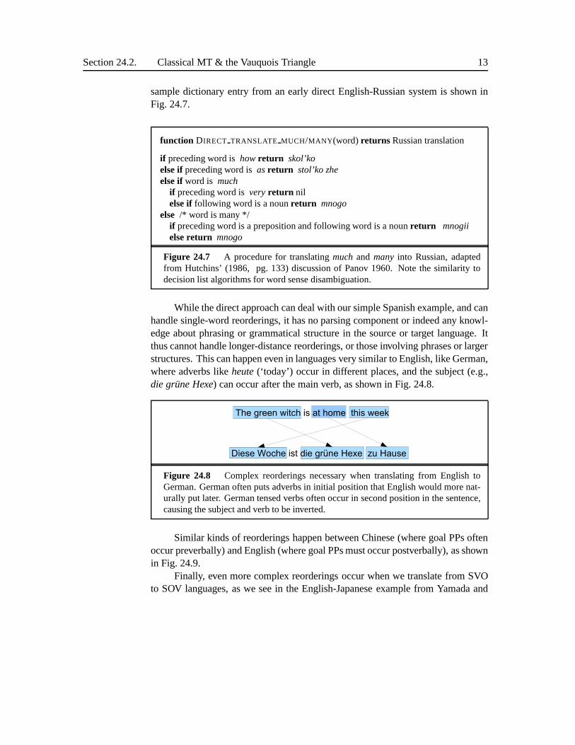
While the direct approach can deal with our simple Spanish example, and canhandle single-word reorderings, it has no parsing component or indeed any knowl-edge about phrasing or grammatical structure in the source or target language. Itthus cannot handle longer-distance reorderings, or those involving phrases or largerstructures. This can happen even in languages very similar to English, like German,where adverbs likeheute(‘today’) occur in different places, and the subject (e.g.,die grune Hexe) can occur after the main verb, as shown in Fig. 24.8.
Figure 24.8 Complex reorderings necessary when translating from English toGerman. German often puts adverbs in initial position that English would more nat-urally put later. German tensed verbs often occur in second position in the sentence,causing the subject and verb to be inverted.
Similar kinds of reorderings happen between Chinese (wheregoal PPs oftenoccur preverbally) and English (where goal PPs must occur postverbally), as shownin Fig. 24.9.
Finally, even more complex reorderings occur when we translate from SVOto SOV languages, as we see in the English-Japanese example from Yamada and

14 Chapter 24. Machine Translation
Figure 24.9 Chinese goal PPs often occur preverbally, unlike in English.
Knight (2002):
(24.12) He adores listening to musickarehe
ha ongakumusic
woto
kikulistening
no ga daisukiadores
desu
These three examples suggest that the direct approach is toofocused on indi-vidual words, and that in order to deal with real examples we’ll need to add phrasaland structural knowledge into our MT models. We’ll flesh out this intuition in thenext section.
24.2.2 Transfer
As Sec. 24.1 illustrated, languages differ systematicallyin structural ways. Onestrategy for doing MT is to translate by a process of overcoming these differences,altering the structure of the input to make it conform to the rules of the target lan-guage. This can be done by applyingcontrastive knowledge, that is, knowledgeCONTRASTIVE
KNOWLEDGE
about the differences between the two languages. Systems that use this strategy aresaid to be based on thetransfer model.TRANSFER MODEL
The transfer model presupposes a parse of the source language, and is fol-lowed by a generation phase to actually create the output sentence. Thus, on thismodel, MT involves three phases:analysis, transfer, andgeneration, where trans-fer bridges the gap between the output of the source languageparser and the inputto the target language generator.
It is worth noting that a parse for MT may differ from parses required forother purposes. For example, suppose we need to translateJohn saw the girl withthe binocularsinto French. The parser does not need to bother to figure out wherethe prepositional phrase attaches, because both possibilities lead to the same Frenchsentence.
Once we have parsed the source language, we’ll need rules forsyntactictransfer andlexical transfer. The syntactic transfer rules will tell us how to mod-ify the source parse tree to resemble the target parse tree.
Figure 24.10 gives an intuition for simple cases like adjective-noun reorder-ing; we transform one parse tree, suitable for describing anEnglish phrase, into

Section 24.2. Classical MT & the Vauquois Triangle 15
noun phrase
adjective noun
noun phrase
adjectivenoun
Figure 24.10 A simple transformation that reorders adjectives and nouns
another parse tree, suitable for describing a Spanish sentence. Thesesyntactictransformations are operations that map from one tree structure to another.SYNTACTIC
TRANSFORMATIONS
The transfer approach and this rule can be applied to our example Mary didnot slap the green witch. Besides this transformation rule, we’ll need to assumethat the morphological processing figures out thatdidn’t is composed ofdo-PASTplusnot, and that the parser attaches the PAST feature onto the VP. Lexical transfer,via lookup in the bilingual dictionary, will then removedo, changenot to no, andturn slap into the phrasedar una bofetada a, with a slight rearrangement of theparse tree, as suggested below:
VP[+PAST]
Neg
not
V
slap
NP
DT
the
JJ
green
NN
witch
⇒ VP[+PAST]
Neg
not
V
slap
NP
DT
the
NN
witch
JJ
green
⇒ VP[+PAST]
Neg
no
V
dar
NP
DT
una
NN
bofetada
PP
IN
a
NP
DT
la
NN
bruja
JJ
verdeFor translating from SVO languages like English to SOV languages like
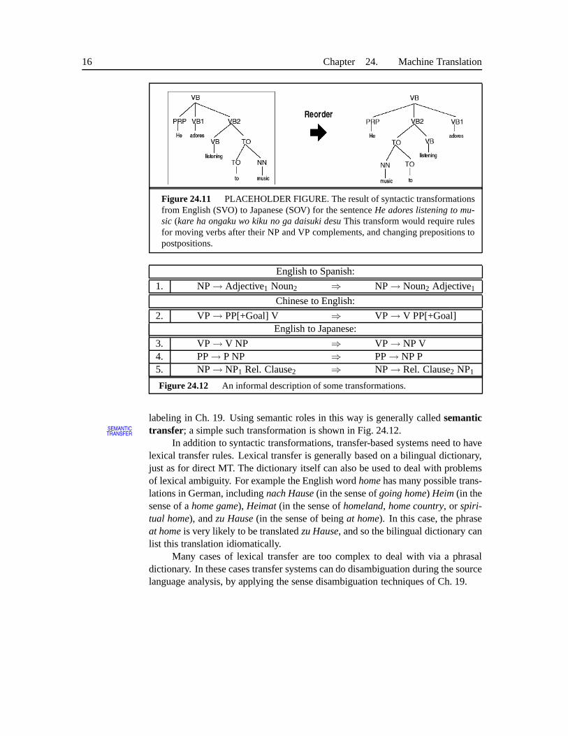
Japanese, we’ll need even more complex transformations, for moving the verb tothe end, changing prepositions into postpositions, and so on. An example of theresult of such rules is shown in Fig. 24.11. An informal sketch of some transferrules is shown in Fig. 24.12.
Transfer systems can be based on richer structures than justpure syntacticparses. For example a transfer based system for translatingChinese to Englishmight have rules to deal with the fact shown in Fig. 24.9 that in Chinese PPs thatfill the semantic roleGOAL (like to the storein I went to the store) tend to appearbefore the verb, while in English these goal PPs must appear after the verb. In orderto build a transformation to deal with this and related PP ordering differences, theparse of the Chinese must including thematic structure, so as to distinguishBENE-FACTIVE PPs (which must occur before the verb) fromDIRECTION andLOCATIVE
PPs (which preferentially occur before the verb) fromRECIPIENTPPs (which occurafter) (Li and Thompson, 1981). We discussed how to do this kind of semantic role
16 Chapter 24. Machine Translation
Figure 24.11 PLACEHOLDER FIGURE. The result of syntactic transformationsfrom English (SVO) to Japanese (SOV) for the sentenceHe adores listening to mu-sic (kare ha ongaku wo kiku no ga daisuki desuThis transform would require rulesfor moving verbs after their NP and VP complements, and changing prepositions topostpositions.
English to Spanish:
1. NP→ Adjective1 Noun2 ⇒ NP→ Noun2 Adjective1
Chinese to English:
2. VP→ PP[+Goal] V ⇒ VP→ V PP[+Goal]English to Japanese:
3. VP→ V NP ⇒ VP→ NP V4. PP→ P NP ⇒ PP→ NP P5. NP→ NP1 Rel. Clause2 ⇒ NP→ Rel. Clause2 NP1
Figure 24.12 An informal description of some transformations.
labeling in Ch. 19. Using semantic roles in this way is generally called semantictransfer; a simple such transformation is shown in Fig. 24.12.SEMANTIC
TRANSFER
In addition to syntactic transformations, transfer-basedsystems need to havelexical transfer rules. Lexical transfer is generally based on a bilingual dictionary,just as for direct MT. The dictionary itself can also be used to deal with problemsof lexical ambiguity. For example the English wordhomehas many possible trans-lations in German, includingnach Hause(in the sense ofgoing home) Heim(in thesense of ahome game), Heimat(in the sense ofhomeland, home country, or spiri-tual home), andzu Hause(in the sense of beingat home). In this case, the phraseat homeis very likely to be translatedzu Hause, and so the bilingual dictionary canlist this translation idiomatically.
Many cases of lexical transfer are too complex to deal with via a phrasaldictionary. In these cases transfer systems can do disambiguation during the sourcelanguage analysis, by applying the sense disambiguation techniques of Ch. 19.

Section 24.2. Classical MT & the Vauquois Triangle 17
24.2.3 Combining direct and tranfer approaches in classic MT
Although the transfer metaphor offers the ability to deal with more complex sourcelanguage phenomena than the direct approach, it turns out the simple SVO→SOV rules we’ve described above are not sufficient. In practice, we need messyrules which combine rich lexical knowledge of both languages with syntactic andsemantic features. We briefly saw an example of such a rule forchangingslap todar una bofetada a.
For this reason, commercial MT systems tend to be combinations of the directand transfer approaches, using rich bilingual dictionaries, but also using taggersand parsers. The Systran (?) system, for example, as described in Hutchins andSomers (1992), has three components. First is a shallowparsing stage, including:
• part of speech tagging• chunking of NPs, PPs, and larger phrases• shallow dependency parsing (subjects, passives, head-modifiers)
Next is atransfer phase, including:
• translation of idioms,• word sense disambiguation• assigning prepositions based on governing verbs
Finally, in thesynthesisstage, the system:
• applies a rich bilingual dictionary to do lexical translation• deals with reorderings• performs morphological generation
Thus like the direct system, the Systran system relies for much of its process-ing on the bilingual dictionary, which has lexical, syntactic, and semantic knowl-edge. Also like a direct system, Systran does reordering in apost-processing step.But like a transfer system, many of the steps are informed by syntactic and shallowsemantic processing of the source language.
24.2.4 The Interlingua Idea: Using Meaning
One problem with the transfer model is that it requires a distinct set of transferrules for each pair of languages. This is clearly suboptimalfor translation systemsemployed in many-to-many multilingual environments like the European Union.
This suggests a different perspective on the nature of translation. Insteadof directly transforming the words of the source language sentence into the targetlanguage, the interlingua intuition is to treat translation as a process of extractingthe meaning of the input and then expressing that meaning in the target language. If

18 Chapter 24. Machine Translation
EVENT SLAPPING
AGENT MARY
TENSE PAST
POLARITY NEGATIVE
THEME
WITCH
DEFINITENESS DEF
ATTRIBUTES[
HAS-COLOR GREEN]
Figure 24.13 Interlingual representation ofMary did not slap the green witch.
this could be done, an MT system could do without contrastiveknowledge, merelyrelying on the same syntactic and semantic rules used by a standard interpreterand generator for the language. The amount of knowledge needed would then beproportional to the number of languages the system handles,rather than to thesquare.
This scheme presupposes the existence of a meaning representation, or in-terlingua, in a language-independent canonical form, like the semantic represen-INTERLINGUA
tations we saw in Ch. 16. The idea is for the interlingua to represent all sentencesthat mean the “same” thing in the same way, regardless of the language they happento be in. Translation in this model proceeds by performing a deep semantic analy-sis on the input from language X into the interlingual representation and generatingfrom the interlingua to language Y.
What kind of representation scheme can we use as an interlingua? The predi-cate calculus, or a variant such as Minimal Recursion semantics, is one possibility.Semantic decomposition into some kind of atomic semantic primitives is another.We will illustrate a third common approach, a simple event-based representation, inwhich events are linked to their arguments via a small fixed set of thematic roles.Whether we use logics or other representations of events, we’ll need to specifytemporal and aspectual properties of the events, and we’ll also need to representnon-eventive relationships between entities, such as thehas-colorrelation betweengreenandwitch. Fig. 24.13 shows a possible interlingual representation for Marydid not slap the green witchas a unification-style feature structure.
We can create these interlingual representation from the source language textusing thesemantic analyzertechniques of Ch. 17 and Ch. 19; using a semanticrole labeler to discover theAGENT relation betweenMary and theslapevent, or theTHEME relation between thewitch and theslap event. We would also need to dodisambiguation of the noun-modifier relation to recognize that the relationship be-tweengreenandwitch is thehas-colorrelation, and we’ll need to discover that this
Section 24.3. Statistical MT 19
event has negative polarity (from the worddidn’t). The interlingua thus requiresmore analysis work than the transfer model, which only required syntactic pars-ing (or at most shallow thematic role labeling). But generation can now proceeddirectly from the interlingua with no need for syntactic transformations.
In addition to doing without syntactic transformations, the interlingual sys-tem does without lexical transfer rules. Recall our earlierproblem of whether totranslateknowinto French assavoiror connaıtre. Most of the processing involvedin making this decision is not specific to the goal of translating into French; Ger-man, Spanish, and Chinese all make similar distinctions, and furthermore the dis-ambiguation ofknow into concepts such asHAVE-A-PROPOSITION-IN-MEMORY
andBE-ACQUAINTED-WITH-ENTITY is also important for other NLU applicationsthat require word-senses. Thus by using such concepts in an interlingua, a largerpart of the translation process can be done with general language processing tech-niques and modules, and the processing specific to the English-to-French transla-tion task can be eliminated or at least reduced, as suggestedin Fig. 24.3.
The interlingual model has its own problems. For example, inorder to trans-late from Japanese to Chinese the universal interlingua must include concepts suchasELDER-BROTHER andYOUNGER-BROTHER. Using these same concepts trans-lating from German-to-English would then require large amounts of unnecessarydisambiguation. Furthermore, doing the extra work involved by the interlinguacommitment requires exhaustive analysis of the semantics of the domain and for-malization into an ontology. Generally this is only possible in relatively simpledomains based on a database model, as in the air travel, hotelreservation, or restau-rant recommendation domains, where the database definitiondetermines the pos-sible entities and relations. For these reasons, interlingual systems are generallyonly used in sublanguage domains.
24.3 STATISTICAL MT
The three classic architectures for MT (direct, transfer, and interlingua) all provideanswers to the questions of what representations to use and what steps to performto translate. But there is another way to approach the problem of translation: tofocus on the result, not the process. Taking this perspective, let’s consider what itmeans for a sentence to be a translation of some other sentence.
This is an issue to which philosophers of translation have given a lot ofthought. The consensus seems to be, sadly, that it is impossible for a sentencein one language to be a translation of a sentence in other, strictly speaking. For ex-ample, one cannot really translate Hebrewadonai roi (‘the Lord is my shepherd’)into the language of a culture that has no sheep. On the one hand, we can write

20 Chapter 24. Machine Translation
something that is clear in the target language, at some cost in fidelity to the original,something likethe Lord will look after me. On the other hand, we can be faithfulto the original, at the cost of producing something obscure to the target languagereaders, perhaps likethe Lord is for me like somebody who looks after animals withcotton-like hair. As another example, if we translate the Japanese phrasefukakuhansei shite orimasu, aswe apologize, we are not being faithful to the meaningof the original, but if we producewe are deeply reflecting (on our past behavior,and what we did wrong, and how to avoid the problem next time), then our outputis unclear or awkward. Problems such as these arise not only for culture-specificconcepts, but whenever one language uses a metaphor, a construction, a word, or atense without an exact parallel in the other language.
So, true translation, which is both faithful to the source language and naturalas an utterance in the target language, is sometimes impossible. If you are goingto go ahead and produce a translation anyway, you have to compromise. This isexactly what translators do in practice: they produce translations that do tolerablywell on both criteria.
This provides us with a hint for how to do MT. We can model the goal oftranslation as the production of an output that maximizes some value function thatrepresents the importance of both faithfulness and fluency.Statistical MT is thename for a class of approaches that do just this, by building probabilistic modelsof faithfulness and fluency, and then combining these modelsto choose the mostprobable translation. If we chose the product of faithfulness and fluency as ourquality metric, we could model the translation from a sourcelanguage sentenceSto a target language sentenceT as:
best-translationT = argmaxT faithfulness(T,S) fluency(T)
This intuitive equation clearly resembles the Bayesiannoisy channel modelwe’ve seen for speech recognition in Ch. 9. Let’s make the analogy perfect andformalize the noisy channel model for statistical machine translation.
First of all, for the rest of this chapter, we’ll assume we aretranslating froma foreign language sentenceF = f1, f2, ..., fm to English. For some examples we’lluse French as the foreign language, and for others Spanish. But in each case weare translatinginto English (although of course the statistical model also worksfor translating out of English). In a probabilistic model, the best English sentenceE = e1,e2, ...,el is the one whose probabilityP(E|F) is the highest. As is usual inthe noisy channel model, we can rewrite this via Bayes rule:
E = argmaxEP(E|F)
= argmaxEP(F|E)P(E)
P(F)

Section 24.3. Statistical MT 21
= argmaxEP(F|E)P(E)(24.13)
We can ignore the denominatorP(F) inside the argmax since we are choosing thebest English sentence for a fixed foreign sentenceF, and henceP(F) is a con-stant. The resulting noisy channel equation shows that we need two components:a translation model P(F|E), and alanguage modelP(E).TRANSLATION
MODEL
LANGUAGE MODEL
E = argmaxE∈English
translation model︷ ︸︸ ︷
P(F|E)
language model︷ ︸︸ ︷
P(E)(24.14)
Notice that applying the noisy channel model to machine translation requiresthat we think of things backwards, as shown in Fig. 24.14. We pretend that theforeign (source language) inputF we must translate is a corrupted version of someEnglish (target language) sentenceE, and that our task is to discover the hidden(target language) sentenceE that generated our observation sentenceF.
Figure 24.14 The noisy channel model of statistical MT. If we are translating asource language French to a target language English, we haveto think of ’sources’and ’targets’ backwards. We build a model of the generation process from an Englishsentence through a channel to a French sentence. Now given a French sentence totranslate, we pretend it is the output of an English sentencegoing through the noisychannel, and search for the best possible ‘source’ English sentence.
The noisy channel model of statistical MT thus requires three components totranslate from a French sentenceF to an English sentenceE:
• A language modelto computeP(E)
• A translation model to computeP(F|E)
• A decoder, which is givenF and produces the most probableE
Of these three components, we have already introduced the language modelP(E) in Ch. 4. Statistical MT systems are based on the sameN-gram languagemodels as speech recognition and other applications. The language model compo-nent is monolingual, and so acquiring training data is relatively easy.

22 Chapter 24. Machine Translation
The next few sections will therefore concentrate on the other two compo-nents, the translation model and the decoding algorithm.
24.4 P(F |E): THE PHRASE-BASED TRANSLATION MODEL
The job of the translation model, given an English sentenceE and a foreign sen-tenceF, is to assign a probability thatE generatesF. Modern statistical MT isbased on the intuition that a good way to compute these probabilities is by con-sidering the behavior ofphrases. As we see in Fig. 24.15, repeated from page13, entire phrases often need to be translated and moved as a unit. The intuitionof phrase-basedstatistical MT is to use phrases (sequences of words) instead ofPHRASEBASED
single words as the fundamental units of translation.
Figure 24.15 Phrasal reorderings necessary when generating German fromEn-glish; repeated from Fig. 24.8.
There are a wide variety of phrase-based models; in this section we willsketch the model of Koehn et al. (2003). We’ll use a Spanish example, seeing howthe phrase-based model computes the probability P(Maria no daba una bofetada ala bruja verde|Mary did not slap the green witch).
The generative story of phrase-based translation has threesteps. First wegroup the English source words into phrases ¯e1, e2...eI . Next we translate eachEnglish phrase ¯ei into a Spanish phrasef j . Finally each of the Spanish phrases is(optionally) reordered.
The probability model for phrase-based translation relieson a translationprobability and adistortion probability . The factorφ( f j |ei) is the translationprobability of generating Spanish phrasef j from English phrase ¯ei . The reorderingof the Spanish phrases is done by thedistortion probabilityd. Distortion in statis-DISTORTION
tical machine translation refers to a word having a different (‘distorted’) position inthe Spanish sentence than it had in the English sentence. Thedistortion probabilityin phrase-based MT means the probability of two consecutiveEnglish phrases be-ing separated in Spanish by a span (of Spanish words) of a particular length. Moreformally, the distortion is parameterized byd(ai −bi−1), whereai is the start posi-tion of the foreign (Spanish) phrase generated by theith English phrase ¯ei , andbi−1

Section 24.4. P(F|E): the Phrase-Based Translation Model 23
is the end position of the foreign (Spanish) phrase generated by thei−1th Englishphrase ¯ei−1. We can use a very simple distortion probability, in which wesimplyraise some small constantα to the distortion.d(ai −bi−1) = α|ai−bi−1−1|. This dis-tortion model penalizes large distortions by giving lower and lower probability thelarger the distortion.
The final translation model for phrase-based MT is:
P(F|E) =I∏
i=1
φ( fi , ei)d(ai −bi−1)(24.15)
Let’s consider the following particular set of phrases for our example sen-tences:
Position 1 2 3 4 5English Mary did not slap the green witchSpanish Maria no daba una bofetada a la bruja verde
Since each phrase follows directly in order (nothing moves around in thisexample, unlike the German example in (24.15)) the distortions are all 1, and theprobabilityP(F|E) can be computed as:
P(F|E) = P(Maria,Mary)×d(1)×P(no|did not)×d(1)×
P(daba una bofetada|slap)×d(1)×P(a la|the)×d(1)×
P(bruja verde|green witch)×d(1)(24.16)
In order to use the phrase-based model, we need two more things. We need amodel ofdecoding, so we can go from a surface Spanish string to a hidden Englishstring. And we need a model oftraining , so we can learn parameters. We’llintroduce the decoding algorithm in Sec. 24.8. Let’s turn first to training.
How do we learn the simple phrase-based translation probability model in(24.15)? The main set of parameters that needs to be trained is the set of phrasetranslation probabilitiesφ( fi , ei).
These parameters, as well as the distortion constantα, could be set if onlywe had a large bilingual training set, in which each Spanish sentence was pairedwith an English sentence, and if furthermore we knew exactlywhich phrase in theSpanish sentence was translated by which phrase in the English sentence. We callsuch a mapping aphrase alignment.PHRASE ALIGNMENT
The table of phrases above showed an implicit alignment of the phrases forthis sentence, for examplegreen witchaligned withbruja verde. If we had a largetraining set with each pair of sentences labeled with such a phrase alignment, wecould just count the number of times each phrase-pair occurred, and normalize to

24 Chapter 24. Machine Translation
get probabilities:
φ( f , e) =count( f , e)
∑
f count( f , e)(24.17)
We could store each phrase pair( f , e), together with its probabilityφ( f , e),in a largephrase translation table.PHRASE
TRANSLATION TABLE
Alas, we don’t have large hand-labeled phrase-aligned training sets. But itturns that we can extract phrases from another kind of alignment called awordalignment. A word alignment is different than a phrase alignment, because itWORD ALIGNMENT
shows exactly which Spanish word aligns to which English word inside each phrase.We can visualize a word alignment in various ways. Fig. 24.16and Fig. 24.17 showa graphical model and an alignment matrix, respectively, for a word alignment.
Figure 24.16 A graphical model representation of a word alignment between theEnglish and Spanish sentences. We will see later how to extract phrases.
.
Figure 24.17 A alignment matrix representation of a word alignment between theEnglish and Spanish sentences. We will see later how to extract phrases.
.
The next section introduces a few algorithms for deriving word alignments.We then show in Sec. 24.7 how we can extract a phrase table fromword alignments,and finally in Sec. 24.8 how the phrase table can be used in decoding.

Section 24.5. Alignment in MT 25
24.5 ALIGNMENT IN MT
All statistical translation models are based on the idea of aword alignment. AWORD ALIGNMENT
word alignment is a mapping between the source words and the target words in aset of parallel sentences.
Fig. 24.18 shows a visualization of an alignment between theEnglish sen-tenceAnd the program has been implementedand the French sentenceLe pro-gramme aete mis en application. For now, we assume that we already know whichsentences in the English text aligns with which sentences inthe French text.
Figure 24.18 An alignment between an English and a French sentence, afterBrown et al. (1993). Each French word aligns to a single English word.
In principle, we can have arbitrary alignment relationships between the En-glish and French word. But the word alignment models we will present (IBMModels 1 and 3 and the HMM model) make a more stringent requirement, which isthat each French word comes from exactly one English word; this is consistent withFig. 24.18. One advantage of this assumption is that we can represent an alignmentby giving the index number of the English word that the Frenchword comes from.We can thus represent the alignment shown in Fig. 24.18 asA = 2,3,4,5,6,6,6.This is a very likely alignment. A very unlikely alignment, by contrast, might beA = 3,3,3,3,3,3,3.
We will make one addition to this basic alignment idea, whichis to allowwords to appear in the foreign sentence that don’t align to any word in the Englishsentence. We model these words by assuming the existence of aNULL Englishword e0 at position 0. Words in the foreign sentence that are not in the Englishsentence, calledspurious words, may be generated bye0. Fig. 24.19 shows theSPURIOUS WORDS
alignment of spurious Spanisha to English NULL.3
While the simplified model of alignment above disallows many-to-one ormany-to-many alignments, we will discuss more powerful translation models thatallow such alignments. Here are two such sample alignments;in Fig. 24.20 we see
3 While this particulara might instead be aligned to Englishslap, there are many cases of spuriouswords which have no other possible alignment site.

26 Chapter 24. Machine Translation
Figure 24.19 The alignment of thespuriousSpanish worda to the English NULLworde0.
an alignment which is many-to-one; each French word does notalign to a singleEnglish word, although each English word does align to a single French word.
Figure 24.20 An alignment between an English and a French sentence, in whicheach French word does not align to a single English word, but each English wordaligns to one French word. Adapted from Brown et al. (1993).
Fig. 24.21 shows an even more complex example, in which multiple Englishwordsdon’t have any moneyjointly align to the French wordssont demunis. Suchphrasal alignmentswill be necessary for phrasal MT, but it turns out they can’tbe directly generated by the IBM Model 1, Model 3, or HMM word alignmentalgorithms.
Figure 24.21 An alignment between an English and a French sentence, in whichthere is a many-to-many alignment between English and French words. Adaptedfrom Brown et al. (1993).
24.5.1 IBM Model 1
We’ll describe two alignment models in this section: IBM Model 1 and the HMMmodel (we’ll also sketch the fertility-based IBM Model 3 in the advanced section).Both arestatistical alignmentalgorithms. For phrase-based statistical MT, we usethe alignment algorithms just to find the best alignment for asentence pair(F,E),
Section 24.5. Alignment in MT 27
in order to help extract a set of phrases. But it is also possible to use these wordalignment algorithms as a translation modelP(F,E) as well. As we will see, therelationship between alignment and translation can be expressed as follows:
P(F|E) =∑
A
P(F,A|E)
We’ll start with IBM Model 1, so-called because it is the firstand simplest offive models proposed by IBM researchers in a seminal paper (Brown et al., 1993).
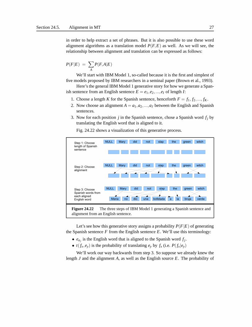
Here’s the general IBM Model 1 generative story for how we generate a Span-ish sentence from an English sentenceE = e1,e2, ...,eI of lengthI :
1. Choose a lengthK for the Spanish sentence, henceforthF = f1, f2, ..., fK .
2. Now choose an alignmentA = a1,a2, ...,aJ between the English and Spanishsentences.
3. Now for each positionj in the Spanish sentence, chose a Spanish wordf j bytranslating the English word that is aligned to it.
Fig. 24.22 shows a visualization of this generative process.
Figure 24.22 The three steps of IBM Model 1 generating a Spanish sentence andalignment from an English sentence.
Let’s see how this generative story assigns a probabilityP(F|E) of generatingthe Spanish sentenceF from the English sentenceE. We’ll use this terminology:
• eaj is the English word that is aligned to the Spanish wordf j .
• t( fx,ey) is the probability of translatingey by fx (i.e. P( fx|ey)
We’ll work our way backwards from step 3. So suppose we already knew thelengthJ and the alignmentA, as well as the English sourceE. The probability of

28 Chapter 24. Machine Translation
the Spanish sentence would be:
P(F|E,A) =J∏
j=1
t( f j |eaj )(24.18)
Now let’s formalize steps 1 and 2 of the generative story. This is the proba-bility P(A|E) of an alignmentA (of lengthJ) given the English sentenceE. IBMModel 1 makes the (very) simplifying assumption that each alignment is equallylikely. How many possible alignments are there between an English sentence oflength I and a Spanish sentence of lengthJ? Again assuming that each Spanishword must come from one of theI English words (or the 1 NULL word), there are(I +1)J possible alignments. Model 1 also assumes that the probability of choosinglengthJ is some small constantε. The combined probability of choosing a lengthJ and then choosing any particular one of the(I +1)J possible alignments is:
P(A|E) =ε
(I +1)J(24.19)
We can combine these probabilities as follows:
P(F,A|E) = P(F|E,A)×P(A|E)
=ε
(I +1)J
J∏
j=1
t( f j |eaj )(24.20)
This probability,P(F,A|E), is the probability of generating a Spanish sen-tenceF via a particular alignment. In order to compute the total probability P(F|E)of generatingF , we just sum over all possible alignments:
P(F|E) =∑
A
P(F,A|E)
=∑
A
ε
(I +1)J
J∏
j=1
t( f j |eaj )(24.21)
Equation (24.21) shows the generative probability model for Model 1, as itassigns a probability to each possible Spanish sentence.
In order to find the best alignment between a pair of sentencesF and E,we need a way todecodeusing this probabilistic model. It turns out there is avery simple polynomial algorithm for computing the best (Viterbi) alignment withModel 1, because the best alignment for each word is independent of the decisionabout best alignments of the surrounding words:
A = argmaxA
P(F,A|E)

Section 24.5. Alignment in MT 29
= argmaxA
ε
(I +1)J
J∏
j=1
t( f j |eaj )
=
[
argmaxaj
t( f j |eaj )
]J
j=1
(24.22)
Training for Model 1 is done by the EM algorithm, which we willcover inSec. 24.6.
24.5.2 HMM Alignment
Now that we’ve seen Model 1, it should be clear that it make some really ap-palling simplifying assumptions. One of the most egregiousis the assumption thatall alignments are equally likely. One way in which this is a bad assumption isthat alignments tend to preservelocality; neighboring words in English are oftenaligned with neighboring words in Spanish. If we look back atthe Spanish/Englishalignment in Fig. 24.16, for example, we can see that this locality in the neigh-boring alignments. The HMM alignment model captures this kind of locality byconditioning each alignment decision on previous decisions. Let’s see how thisworks.
The HMM alignment model is based on the familiar HMM model we’ve nowseen in many chapters. As with IBM Model 1, we are trying to computeP(F,A|E).The HMM model is based on a restructuring of this probabilityusing the chain ruleas follows:
P( f J1 ,aJ
1|eI1) = P(J|eI
1)×J∏
j=1
P( f j ,a j | fj−1
1 ,a j−11 ,eI
1)
= P(J|eI1)×
J∏
j−1
P(a j | fj−1
1 ,a j−11 ,eI
1)×P( f j | fj−1
1 ,a j1,e
I1)(24.23)
Via this restructuring, we can think ofP(F,A|E) as being decomposed intothree probabilities: a length probabilityP(J|eI
1), an alignment probabilityP(a j | fj−1
1 ,a j−11 ,eI
1),and a lexicon probabilityP( f j | f
j−11 ,a j
1,eI1).
We next make some standard Markov simplifying assumptions.We’ll as-sume that the probability of a particular alignmenta j for Spanish wordj is onlydependent on the previous aligned positiona j−1. We’ll also assume that the prob-ability of a Spanish wordf j is dependent only on the aligned English wordeaj atpositiona j :
P(a j | fj−1
1 ,a j−11 ,eI
1 = P(a j |a j−1, I)(24.24)
P( f j | fj−1
1 ,a j1,e
I1 = P( f j |eaj−1)(24.25)

30 Chapter 24. Machine Translation
Finally, we’ll assume that the length probability can be approximated just asP(J|I).
Thus the probabilistic model for HMM alignment is:
P( f J1 ,aJ
1|eI1) = P(J|I)×
J∏
j=1
P(a j |a j−1, I)P( f j |eaj )(24.26)
To get the total probability of the Spanish sentenceP( f J1 |e
I1) we need to sum
over all alignments:
P( f J1 |e
I1) = P(J|I)×
∑
A
J∏
j=1
P(a j |a j−1, I)P( f j |eaj )(24.27)
As we suggested at the beginning of the section, we’ve conditioned the align-ment probabilityP(a j |a j−1, I) on the previous aligned word, to capture the localityof alignments. Let’s rephrase this probability for a momentasP(i|i′, I), whereiwill stand for the absolute positions in the English sentence of consecutive alignedstates the Spanish sentence. We’d like to make these probabilities dependent noton the absolute word positionsi and i′, but rather on thejump width betweenJUMP WIDTH
words; the jump width is the distance between their positions i′− i. This is becauseour goal is to capture the fact that‘the English words that generate neighboringSpanish words are likely to be nearby’. We thus don’t want to be keeping separateprobabilities for each absolute word position likeP(6,5|15) and P(8|7,15). In-stead, we compute alignment probabilities by using a non-negative function of thejump width:
P(i|i′, I) =c(i− i′)
∑Ii′′=1c(i′′− i′)
(24.28)
Let’s see how this HMM model gives the probability of a particular alignmentof our English-Spanish sentences; we’ve simplified the sentence slightly.
Figure 24.23 The HMM alignment model generating fromMary slappped thegreen witch, showing the alignment and lexicon components of the probabilityP(F,A|E) for this particular alignment.

Section 24.6. Training Alignment Models 31
Thus the probabilityP(F,A|E) for this particular alignment of our simplifiedsentenceMaria daba una bofetada a la bruja verdeis the product of:
P(F,A|E) = P(J|I)×P(Maria|Mary)×P(2|1,5)×
t(daba|slapped)×P(2|2,5)×T(una|slapped)×P(2|2,5)× . . .(24.29)
There are also more sophisticated augmentations to the basic HMM align-ment model. These include adding NULL words in the English source which canbe used to align with Spanish words that don’t align with English words, or con-ditioning the alignment onC(eaj−1), the word class of the preceding target word:P(a j |a j−1, I ,C(eaj−1)) (Och and Ney, 2003; Toutanova et al., 2002).
The main advantage of the HMM alignment model is that there are well-understood algorithms both for decoding and for training. For decoding, we canuse the Viterbi algorithm introduced in Ch. 5 and Ch. 6 to find the best (Viterbi)alignment for a sentence pair(F,E). For training, we can use the Baum-Welchalgorithm, as summarized in the next section.
24.6 TRAINING ALIGNMENT MODELS
All statistical translation models are trained using a large parallel corpus. A par-allel corpus, parallel text, or bitext is a text that is available in two languages.PARALLEL CORPUS
BITEXT For example, the proceedings of the Canadian parliament arekept in both Frenchand English. Each sentence spoken in parliament is translated, producing a vol-ume with running text in both languages. These volumes are called Hansards,HANSARDS
after the publisher of the British parliamentary proceedings. Similarly, theHongKong Hansardscorpus contains the proceedings of the Hong Kong SAR Legisla-HONG KONG
HANSARDS
tive Council in both English and Chinese. Both of these corpora contain tens tohundreds of millions of words. Other parallel corpora have been made availableby the United Nations. It is possible to make parallel corpora out of literary trans-lations, but this is less common for MT purposes, partly because it is difficult toacquire the legal rights to fiction, but mainly because, as wesaw at the beginningof the chapter, translating fiction is very difficult and translations are not very lit-eral. Thus statistical systems tend to be trained on very literal translations such asHansards.
The first step in training is to segment the corpus into sentences. This task iscalledsentence segmentationor sentence alignment. The simplest methods alignSENTENCE
SEGMENTATION
SENTENCEALIGNMENT sentences based purely on their length in words or characters, without looking at
the contents of the words in the sentences. The intuition is that if we see a longsentence in roughly the same position in each language of theparallel text, we

32 Chapter 24. Machine Translation
might suspect these sentences are translations. This intuition can be implementedby a dynamic programming algorithm. More sophisticated algorithms also makeuse of information about word alignments. Sentence alignment algorithms are runon a parallel corpus before training MT models. Sentences which don’t align toanything are thrown out, and the remaining aligned sentences can be used as atraining set. See the end of the chapter for pointers to more details on sentencesegmentation.
Once we have done sentence alignment, the input to our training algorithmis a corpus consisting ofSsentence pairs{(Fs,Es) : s= 1. . .S}. For each sentencepair (Fs,Es) the goal is to learn an alignmentA = aJ
1 and the component proba-bilities (t for Model 1, and the lexicon and alignment probabilities forthe HMMmodel).
24.6.1 EM for Training Alignment Models
If each sentence pair(Fs,Es) was already hand-labeled with a perfect alignment,learning the Model 1 or HMM parameters would be trivial. For example, toget a maximum likelihood estimates in Model 1 for the translation probabilityt(verde,green), we would just count the number of timesgreenis aligned toverde,and normalize by the total count ofgreen.
But of course we don’t know the alignments in advance; all we have arethe probabilities of each alignment. Recall that Eq˙ 24.20 showed that if we al-ready had good estimates for the Model 1t parameter, we could use this to computeprobabilitiesP(F,A|E) for alignments. GivenP(F,A|E), we can generate the prob-ability of an alignment just by normalizing:
P(A|E,F) =P(A,F|E)
∑
AP(A,F|E)
So, if we had a rough estimate of the Model 1t parameters, we could computethe probability for each alignment. Then instead of estimating thet probabilitiesfrom the (unknown) perfect alignment, we would estimate them from each possi-ble alignment, and combine these estimates weighted by the probability of eachalignment. For example if there were two possible alignments, one of probability.9 and one of probability .1, we would estimate thet parameters separately fromthe two alignments and mix these two estimates with weights of .9 and .1.
Thus if we had model 1 parameters already, we couldre-estimatethe param-eters, by using the parameters to compute the probability ofeach possible align-ment, and then using the weighted sum of alignments to re-estimate the model 1parameters. This idea of iteratively improving our estimates of probabilities is aspecial case of theEM algorithm that we introduced in Ch. 6, and that we sawagain for speech recognition in Ch. 9. Recall that we use the EM algorithm when

Section 24.6. Training Alignment Models 33
we have a variable that we can’t optimize directly because itis hidden. In this casethe hidden variable is the alignment. But we can use the EM algorithm to estimatethe parameters, compute alignments from these estimates, use the alignments tore-estimate the parameters, and so on!
Let’s walk through an example inspired by Knight (1999b), using a simplifiedversion of Model 1, in which we ignore the NULL word, and we only consider asubset of the alignments (ignoring alignments for which an English word alignswith no Spanish word). Hence we compute the simplified probability P(A,F|E) asfollows:
P(A,F|E) =J∏
j=1
t( f j |eaj )(24.30)
The goal of this example is just to give an intuition of EM applied to this task; theactual details of Model 1 training would be somewhat different.
The intuition of EM training is that in the E-step, we computeexpectedcounts for the t parameter based on summing over the hidden variable (the align-ment), while in the M-step, we compute the maximum likelihood estimate of thetprobability from these counts.
Let’s see a few stages of EM training of this parameter on a a corpus of twosentences:
green house the housecasa verde la casa
The vocabularies for the two languages areE = {green,house,the} andS={casa,la,verde}. We’ll start with uniform probabilities:
t(casa|green) = 13 t(verde|green) = 1
3 t(la|green) = 13
t(casa|house) = 13 t(verde|house) = 1
3 t(la|house) = 13
t(casa|the) = 13 t(verde|the) = 1
3 t(la|the) = 13
Now let’s walk through the steps of EM:
E-step 1: Compute the expected countsE[count(t( f ,e))] for all word pairs( f j ,eaj )
E-step 1a: We first need to computeP(a, f |e), by multiplying all thet probabilities,following Eq. 24.30
green house green house the house the house
casa verde casa verde la casa la casaP(a, f |e) = t(casa,green) P(a, f |e) = t(verde,green) P(a, f |e) = t(la,the) P(a, f |e) = t(casa,the)× t(verde,house) × t(casa,house) × t(casa,house) × t(la,house)
= 13×
13 = 1
9 = 13 ×
13 = 1
9 = 13×
13 = 1
9 = 13 ×
13 = 1
9

34 Chapter 24. Machine Translation
E-step 1b: NormalizeP(a, f |e) to getP(a|e, f ), using the following:
P(a|e, f ) =P(a, f |e)
∑
a P(a, f |e)
The resulting values ofP(a| f ,e) for each alignment are as follows:
green house green house the house the house
casa verde casa verde la casa la casaP(a| f ,e) =
1/92/9 = 1
2 P(a| f ,e) =1/92/9 = 1
2 P(a| f ,e) =1/92/9 = 1
2 P(a| f ,e) =1/92/9 = 1
2
E-step 1c: Compute expected (fractional) counts, by weighting each count byP(a|e, f )
tcount(casa|green) = 12 tcount(verde|green) = 1
2 tcount(la|green) = 0 total(green) = 1
tcount(casa|house) = 12 + 1
2 tcount(verde|house) = 12 tcount(la|house) = 1
2 total(house) = 2
tcount(casa|the) = 12 tcount(verde|the) = 0 tcount(la|the) = 1
2 total(the) = 1
M-step 1: Compute the MLE probability parameters by normalizing the tcounts to sum toone.
t(casa|green) = 1/21 = 1
2 t(verde|green) = 1/21 = 1
2 t(la|green) = 01 = 0
t(casa|house) = 12 = 1
2 t(verde|house) = 1/22 = 1
4 t(la|house) = 1/22 = 1
4
t(casa|the) = 1/21 = 1
2 t(verde|the) = 01 = 0 t(la|the) = 1/2
1 = 12
Note that each of the correct translations have increased inprobability fromthe initial assignment; for example the translationcasafor househas increased inprobability from 1
3 to 12.
E-step 2a: We re-computeP(a, f |e), again by multiplying all thet probabilities, followingEq. 24.30
green house green house the house the house
casa verde casa verde la casa la casaP(a, f |e) = t(casa,green) P(a, f |e) = t(verde,green) P(a, f |e) = t(la,the) P(a, f |e) = t(casa,the)× t(verde,house) × t(casa,house) × t(casa,house) × t(la,house)
= 12×
14 = 1
8 = 12 ×
12 = 1
4 = 12×
12 = 1
4 = 12 ×
14 = 1
8
Note that the two correct alignments are now higher in probability than thetwo incorrect alignments. Performing the second and further round of E-steps andM-steps is left as Exercise 24.6 for the reader.
We have shown that EM can be used to learn the parameters for a simplifiedversion of Model 1. Our intuitive algorithm, however, requires that we enumerate
Section 24.7. Symmetrizing Alignments for Phrase-based MT 35
all possible alignments. For a long sentence, enumerating every possible alignmentwould be very inefficient. Luckily in practice there is a veryefficient version of EMfor Model 1 that efficiently and implicitly sums over all alignments.
We also use EM, in the form of the Baum-Welch algorithm, for learning theparameters of the HMM model.
24.7 SYMMETRIZING ALIGNMENTS FORPHRASE-BASED MT
The reason why we needed Model 1 or HMM alignments was to buildword align-ments on the training set, so that we could extract aligned pairs of phrases.
Unfortunately, HMM (or Model 1) alignments are insufficientfor extractingpairings of Spanish phrases with English phrases. This is because in the HMMmodel, each Spanish word must be generated from a single English word; we can-not generate a Spanish phrase from multiple English words. The HMM model thuscannot align a multiword phrase in the source language with amultiword phrase inthe target language.
We can, however, extend the HMM model to produce phrase-to-phrase align-ments for a pair of sentences(F,E), via a method that’s often calledsymmetriz-ing. First, we train two separate HMM aligners, an English-to-Spanish aligner andSYMMETRIZING
a Spanish-to-English aligner. We then align (F ,E) using both aligners. We can thencombine these alignments in clever ways to get an alignment that maps phrases tophrases.
To combine the alignments, we start by taking theintersection of the twoINTERSECTION
alignments, as shown in Fig. 24.24. The intersection will contain only places wherethe two alignments agree, hence the high-precision alignedwords. We can alsoseparately compute theunion of these two alignments. The union will have lotsof less accurately aligned words. We can then build a classifier to select wordsfrom the union, which we incrementally add back in to this minimal intersectivealignment.
Fig. 24.25 shows an example of the resulting word alignment.Note that itdoes allow many-to-one alignments in both directions. We can now harvest allphrase pairs that are consistent with this word alignment. Aconsistent phrase pairis one in which all the words are aligned only with each other,and not to anyexternal words. Fig. 24.25 also shows some phrases consistent with the alignment.
Once we collect all the aligned phrases pairs from the entiretraining cor-pus, we can compute the maximum likelihood estimate for the phrase translationprobability of a particular pair as follows:
φ( f , e) =count( f , e)
∑
f count( f , e)(24.31)

36 Chapter 24. Machine Translation
Figure 24.24 PLACEHOLDER FIGURE, from (Koehn, 2003b). Intersection ofEnglish-to-Spanish and Spanish-to-English alignments toproduce a high-precisionalignment. Alignment can then be expanded with points from both alignments toproduce an alignment like that shown in Fig. 24.25.
(Maria, Mary), (no, did not),(slap, daba una bofetada), (verde, green),(a la, the), (bruja, witch),(Maria no, Mary did not),(no daba una bofetada, did not slap),(daba una bofetada a la, slap the),(bruja verde, green witch),(a la bruja verde, the green witch),. . .
Figure 24.25 A better phrasal alignment for thegreen witchsentence, computedby starting with the intersection alignment in Fig. 24.24 and adding points from theunion alignment, using the algorithm of ? (?). On the right, some of the phrasesconsistent with this alignment, after Koehn (2003b).
We can now store each phrase( f , e), together with its probabilityφ( f , e), ina largephrase translation table. The decoding algorithm discussed in the nextPHRASE
TRANSLATION TABLE

Section 24.8. Decoding for Phrase-Based Statistical MT 37
section can use this phrase translation table to compute thetranslation probability.
24.8 DECODING FORPHRASE-BASED STATISTICAL MT
The remaining component of a statistical MT system is the decoder. Recall thatthe job of the decoder is to take a foreign (Spanish) source sentenceF and producethe best (English) translationE according to the product of the translation andlanguage models:
E = argmaxE∈English
translation model︷ ︸︸ ︷
P(F|E)
language model︷ ︸︸ ︷
P(E)(24.32)
Finding the sentence which maximizes the translation and language modelprobabilities is asearchproblem, and decoding is thus a kind of search. Decodersin MT are based onbest-first search, a kind ofheuristic or informed search; theseare search algorithms that are informed by knowledge from the problem domain.Best-first search algorithms select a noden in the search space to explore basedon an evaluation functionf (n). MT decoders are variants of a specific kind ofbest-first search calledA∗ search. A∗ search was first implemented for machinetranslation by IBM (Brown et al., 1995), based on IBM’s earlier work on A∗ searchfor speech recognition (Jelinek, 1969). As we discussed in Sec.??, for historicalreasons A∗ search and its variants are commonly calledstack decodingin speechSTACK DECODING
recognition and sometimes also in machine translation.Let’s begin in Fig. 24.26 with a generic version of stack decoding for ma-
chine translation. The basic intuition is to maintain apriority queue (traditionallyreferred to as astack) with all the partial translation hypotheses, together with theirscores.
Let’s now describe stack decoding in more detail. While the original IBMstatistical decoding algorithms were for word-based statistical MT, we will de-scribe the application to phrase-based decoding in the publicly available MT de-coderPharaoh (Koehn, 2004).
In order to limit the search space in decoding, we don’t want to search throughthe space of all English sentences; we only want to consider the ones that are pos-sible translations forF. To help reduce the search space, we only want to considersentences that include words or phrases which are possible translations of words orphrases in the Spanish sentenceF. We do this by searching thephrase translationtable described in the previous section, for all possible Englishtranslations for allpossible phrases inF.
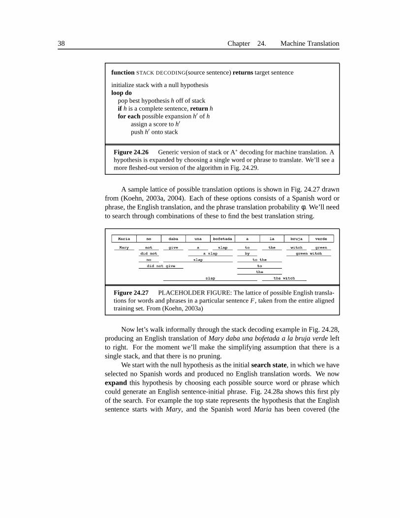
38 Chapter 24. Machine Translation
function STACK DECODING(source sentence)returns target sentence
initialize stack with a null hypothesisloop do
pop best hypothesish off of stackif h is a complete sentence,return hfor eachpossible expansionh′ of h
assign a score toh′
pushh′ onto stack
Figure 24.26 Generic version of stack or A∗ decoding for machine translation. Ahypothesis is expanded by choosing a single word or phrase totranslate. We’ll see amore fleshed-out version of the algorithm in Fig. 24.29.
A sample lattice of possible translation options is shown inFig. 24.27 drawnfrom (Koehn, 2003a, 2004). Each of these options consists ofa Spanish word orphrase, the English translation, and the phrase translation probabilityφ. We’ll needto search through combinations of these to find the best translation string.
Figure 24.27 PLACEHOLDER FIGURE: The lattice of possible English transla-tions for words and phrases in a particular sentenceF , taken from the entire alignedtraining set. From (Koehn, 2003a)
Now let’s walk informally through the stack decoding example in Fig. 24.28,producing an English translation ofMary daba una bofetada a la bruja verdeleftto right. For the moment we’ll make the simplifying assumption that there is asingle stack, and that there is no pruning.
We start with the null hypothesis as the initialsearch state, in which we haveselected no Spanish words and produced no English translation words. We nowexpand this hypothesis by choosing each possible source word or phrase whichcould generate an English sentence-initial phrase. Fig. 24.28a shows this first plyof the search. For example the top state represents the hypothesis that the Englishsentence starts withMary, and the Spanish wordMaria has been covered (the
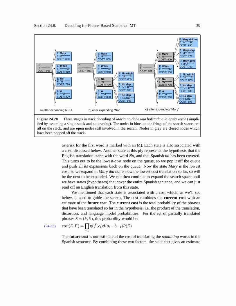
Section 24.8. Decoding for Phrase-Based Statistical MT 39
Figure 24.28 Three stages in stack decoding ofMaria no daba una bofetada a la bruja verde(simpli-fied by assuming a single stack and no pruning). The nodes in blue, on the fringe of the search space, areall on the stack, and areopen nodes still involved in the search. Nodes in gray areclosednodes whichhave been popped off the stack.
asterisk for the first word is marked with an M). Each state is also associated witha cost, discussed below. Another state at this ply represents the hypothesis that theEnglish translation starts with the wordNo, and that Spanishno has been covered.This turns out to be the lowest-cost node on the queue, so we pop it off the queueand push all its expansions back on the queue. Now the stateMary is the lowestcost, so we expand it;Mary did notis now the lowest cost translation so far, so willbe the next to be expanded. We can then continue to expand the search space untilwe have states (hypotheses) that cover the entire Spanish sentence, and we can justread off an English translation from this state.
We mentioned that each state is associated with a cost which,as we’ll seebelow, is used to guide the search, The cost combines thecurrent cost with anestimate of thefuture cost. Thecurrent cost is the total probability of the phrasesthat have been translated so far in the hypothesis, i.e. the product of the translation,distortion, and language model probabilities. For the set of partially translatedphrasesS= (F,E), this probability would be:
cost(E,F) =∏
i∈S
φ( fi , ei)d(ai −bi−1)P(E)(24.33)
Thefuture cost is our estimate of the cost of translating theremainingwords in theSpanish sentence. By combining these two factors, the statecost gives an estimate

40 Chapter 24. Machine Translation
of the total probability of the search path for the eventual complete translationsentenceE passing through the current node. A search algorithm based only on thecurrent cost would tend to select translations that had a fewhigh-probability wordsat the beginning, at the expense of translations with a higher overall probability.4 For the future cost, it turns out to be far too expensive to compute the trueminimum probability for all possible translations. Instead, we approximate thiscost by ignoring the distortion cost and just finding the sequence of English phraseswhich has the minimum product of the language model and translation model costs,which can be easily computed by the Viterbi algorithm.
This sketch of the decoding process suggests that we search the entire statespace of possible English translations. But we can’t possibly afford to expand theentire search space, because there are far too many states; unlike in speech recog-nition, the need for distortion in MT means there is (at least) a distinct hypothesisfor every possible ordering of the English words!5
For this reason MT decoders, like decoders for speech recognition, all requiresome sort of pruning. Pharaoh and similar decoders use a version of beam-searchpruning , just as we saw in decoding for speech recognition and probabilistic pars-BEAMSEARCH
PRUNING
ing. Recall that in beam-search pruning, at every iterationwe keep only the mostpromising states, and prune away unlikely (high-cost) states (those ‘outside thesearch beam’). We could modify the search sequence depictedin Fig. 24.28, bypruning away all bad (high-cost) states at every ply of the search, and expandingonly the best state. In fact, in Pharaoh, instead of expanding only the best state, weexpand all states within the beam; thus Pharaoh is technically beam searchratherthanbest-first searchor A∗ search.
More formally, at each ply of the search we keep around a stack(priorityqueue) of states. The stack only fitsn entries. At every ply of the search, weexpand all the states on the stack, push them onto the stack, order them by cost,keep the bestn entries and delete the rest.
We’ll need one final modification. While in speech we just usedone stack forstack decoding, in MT we’ll use multiple stacks, because we can’t easily comparethe cost of hypotheses that translate different numbers of foreign words. So we’llusem stacks, where stacksm includes all hypotheses that coverm foreign words.When we expand a hypothesis by choosing a phrase to translate, we’ll insert thenew state into the correct stack for the number of foreign words covered. Thenwe’ll use beam-search inside each of these stacks, keep onlyn hypotheses for eachof the m stacks. The final multi-stack version of beam search stack decoding is
4 We saw this same kind of cost function for A∗ search in speech recognition, where we used theA∗ evaluation function:f ∗(p) = g(p)+h∗(p).5 Indeed, as Knight (1999a) shows, decoding even in IBM Model 1with a bigram language modelis equivalent to the difficult class of problems known asNP-complete.

Section 24.8. Decoding for Phrase-Based Statistical MT 41
shown in Fig. 24.29.
function BEAM SEARCH STACK DECODER(source sentence)returns target sentence
initialize hypothesisStack[0..nf]push initial null hypothesis on hypothesisStack[0]for i←0 tonf-1
for eachhyp in hypothesisStack[i]for eachnewhypthat can be derived fromhyp
nf[newhyp]←number of foreign words covered bynewhypaddnewhypto hypothesisStack[nf[newhyp]]prune hypothesisStack[nf[newhyp]]
find best hypothesisbesthypin hypothesisStack[nf]return best path that leads tobesthypvia backtrace
Figure 24.29 Pharaoh beam search multi-stack decoding algorithm, adapted from(Koehn, 2003a, 2004). For efficiency, most decoders don’t store the entire foreignand English sentence in each state, requiring that we backtrace to find the state pathfrom the initial to the final state so we can generate the entire English target sentence.
There are a number of additional issues in decoding that mustbe dealt with.All decoders attempt to limit somewhat the exponential explosion in the searchspace byrecombining hypotheses. We saw hypothesis recombination in theExactRECOMBINING
HYPOTHESES
N-Best algorithm of Sec.??. In MT, we can merge any two hypotheses that aresufficiently similar (cover the same foreign words, have thesame last-two Englishwords, and have the same end of the last foreign phrase covered).
In addition, it turns out that decoders for phrasal MT optimize a slightly dif-ferent function than the one we presented in Eq. 24.32. In practice, it turns out thatwe need to add another factor, which serves to penalize sentences which are tooshort. Thus the decoder is actually choosing the sentence which maximizes:
E = argmaxE∈English
translation model︷ ︸︸ ︷
P(F|E)
language model︷ ︸︸ ︷
P(E)
short sentence penalty︷ ︸︸ ︷
ωlength(E)(24.34)
This final equation is extremely similar to the use of the wordinsertionpenalty in speech recognition in Eq.??.

42 Chapter 24. Machine Translation
24.9 MT EVALUATION
Evaluating the quality of a translation is an extremely subjective task, and dis-agreements about evaluation methodology are rampant. Nevertheless, evaluationis essential, and research on evaluation methodology has played an important rolein earliest days of MT (Miller and Beebe-Center, 1958) and inthe present. Broadlyspeaking, we attempt to evaluate translations along two dimensions, correspondingto thefidelity andfluencydiscussed in Sec. 24.3.
24.9.1 Using Human Raters
The most accurate evaluations use human raters to evaluate each translation alongeach dimension. For example, along the dimension offluency, we can ask howintelligible, how clear, how readable, or how natural is theMT output (the targettranslated text). There are two broad ways to use human raters to answer thesequestions. One method is to give the raters a scale, for example from 1 (totallyunintelligible) to 5 (totally intelligible), and ask them to rate each sentence or para-graph of the MT output. We can use distinct scales for any of the aspects of fluency,such asclarity , naturalness, or style (?). The second class of methods relies lesson the conscious decisions of the participants. For example, we can measure thetime it takes for the raters to read each output sentence or paragraph. Clearer ormore fluent sentences should be faster or easier to read. We can also measure flu-ency with theclozetask (?). The cloze task is a metric used often in psychologicalCLOZE
studies of reading. The rater sees an output sentence with a word replaced by aspace (for example, every 8th word might be deleted). Ratershave to guess theidentity of the missing word. Accuracy at the cloze task, i.e. average success ofraters at guessing the missing words, generally correlateswith how intelligible ornatural the MT output is.
A similar variety of metrics can be used to judge the second dimension,fi-delity. Two common aspects of fidelity which are measured areadequacyandinformativeness. Theadequacyof a translation is whether it contains the infor-ADEQUACY
mation that existed in the original. We measureadequacyby using raters to assignADEQUACY
scores on a scale. If we have bilingual raters, we can give them the source sentenceand a proposed target sentence, and rate, perhaps on a 5-point scale, how much ofthe information in the source was preserved in the target. Ifwe only have monolin-gual raters, but we have a good human translation of the source text, we can givethe monolingual raters the human reference translation anda target machine trans-lation, and again rate how much information is preserved. The informativenessINFORMATIVENESS
of a translation is a task-based evaluation of whether thereis sufficient informationin the MT output to perform some task. For example we can give raters multiple-

Section 24.9. MT Evaluation 43
choice questions about the content of the material in the source sentence or text.The raters answer these questions based only on the MT output. The percentage ofcorrect answers is an informativeness score.
Another set of metrics attempt to judge the overall quality of a translation,combining fluency and fidelity. For example, the typical evaluation metric for MToutput to be post-edited is theedit costof post-editing the MT output into a goodEDIT COST
POSTEDITING translation. For example, we can measure the number of words, the amount oftime, or the number of keystrokes required for a human to correct the output to anacceptable level.
24.9.2 Automatic Evaluation: Bleu
While humans produce the best evaluations of machine translation output, runninga human evaluation can be very time-consuming, taking days or even weeks. It isuseful to have an automatic metric that can be run relativelyfrequently to quicklyevaluate potential system improvements. In order to have such convenience, wewould be willing for the metric to be much worse than human evaluation, as longas there was some correlation with human judgments.
In fact there are a number of such heuristic methods, such asBleu, NIST,Precision and Recall, andMETEOR (see references at the end of the chapter).The intuition of these automatic metrics derives from Miller and Beebe-Center(1958), who pointed out that a good MT output is one which is very similar to ahuman translation. For each of these metrics, we assume thatwe already have oneor more human translations of the relevant sentences. Now given an MT outputsentence, we compute the translation closeness between theMT output and thehuman sentences. An MT output is ranked as better if on average it is closer to thehuman translations. The metrics differ on what counts as ‘translation closeness’.
In the field of automatic speech recognition, the metric for ‘transcriptioncloseness’ is word error rate, which is the minimum edit distance to a human tran-script. But in translation, we can’t use the same word error rate metric, becausethere are many possible translations of a source sentence; avery good MT outputmight look like one human translation, but very unlike another one. For this rea-son, most of the metrics judge an MT output by comparing it to multiple humantranslations.
Each of these metrics thus require that we get human translations in advancefor a number of test sentences. This may seem time-consuming, but the hope isthat we can reuse this translated test set over and over againto evaluate new ideas.
For the rest of this section, let’s walk through one of these metrics, theBleumetric, following closely the original presentation in Papineni et al. (2002). In Bleuwe rank each MT output by a weighted average of the number ofN-gram overlaps

44 Chapter 24. Machine Translation
with the human translations.Fig. 24.30 shows an intuition, from two candidate translations of a Chinese
source sentence (Papineni et al., 2002), shown with three reference human trans-lations of the source sentence. Note that Candidate 1 sharesmany more words(shown in blue) with the reference translations than Candidate 2.
Figure 24.30 Intuition for Bleu: one of two candidate translations of a Chinese source sentence sharesmore words with the reference human translations.
Let’s look at how the Bleu score is computed, starting with just unigrams.Bleu is based on precision. A basic unigram precision metricwould be to countthe number the words in the candidate translation (MT output) that occur in somereference translation, and divide by the total number of words in the candidatetranslation. If a candidate translation had 10 words, and 6 of them occurred in atleast one of the reference translations, we would have a precision of 6/10 = 0.6.Alas, there is a flaw in using simple precision: it rewards candidates that haveextra repeated words. Fig. 24.31 shows an example of a pathological candidatesentence composed of multiple instances of the single wordthe. Since each of the7 (identical) words in the candidate occur in one of the reference translations, theunigram precision would be 7/7!
Figure 24.31 A pathological example showing why Bleu uses a modified preci-sion metric. Unigram precision would be unreasonably high (7/7). Modified unigramprecision is appropriately low (2/7).
In order to avoid this problem, Bleu uses amodified N-gram precision met-MODIFIED NGRAMPRECISION

Section 24.9. MT Evaluation 45
ric. We first count the maximum number of times a word is used inany singlereference translation. The count of eachcandidateword is then clipped by thismaximumreferencecount. Thus the modified unigram precision in the example inFig. 24.31 would be 2/7, since Reference 1 has a maximum of 2thes. Going backto Chinese example in Fig. 24.31, Candidate 1 has a modified unigram precisionof 17/18, while Candidate 2 has one of 8/14.
We compute the modified precision similarly for higher ordern-grams aswell. The modified bigram precision for Candidate 1 is 10/17,and for Candidate 2is 1/13. The reader should check these numbers for themselves on Fig. 24.30.
To compute a score over the whole testset, Bleu first computesthe N-grammatches for each sentence, and add together the clipped counts over all the candi-dates sentences, and divide by the total number of candidateN-grams in the testset.The modified precision score is thus:
pn =
∑
C∈{Candidates}
∑
n-gram∈C
Countclip(n-gram)
∑
C′∈{Candidates}
∑
n-gram∈C′Count(n-gram’)
(24.35)
Bleu uses unigram, bigrams, trigrams, and often quadrigrams; it combinesthese modifiedN-gram precisions together by taking their geometric mean.
In addition, Bleu adds a further penalty to penalize candidate translations thatare too short. Consider the candidate translationof the, compared with References1-3 in Fig. 24.30 above. Because this candidate is so short, and all its words appearin some translation, its modified unigram precision is inflated to 2/2. Normally wedeal with these problems by combining precision withrecall. But as we discussedabove, we can’t use recall over multiple human translations, since recall wouldrequire (incorrectly) that a good translation must containcontains lots ofN-gramsfrom every translation. Instead, Bleu includes a brevity penalty overthe wholecorpus. Letc be the total length of the candidate translation corpus. We computethe effective reference lengthr for that corpus by summing, for each candidatesentence, the lengths of the best matches. The brevity penalty is then an exponentialin r/c. In summary:
BP =
{
1 if c > re(1−r/c) if c≤ r
Bleu = BP×exp
(N∑
n=1
logpn
)
(24.36)
While automatic metrics like Bleu (or NIST, METEOR, etc) have been veryuseful in quickly evaluating potential system improvements, and match human

46 Chapter 24. Machine Translation
judgments in many cases, they have certain limitations thatare important to con-sider. First, many of them focus on very local information. Consider slightly mov-ing a a phrase in Fig. 24.30 slightly to produce a candidate like: Ensures that themilitary it is a guide to action which always obeys the commands of the party. Thissentence would have an identical Bleu score to Candidate 1, although a humanrater would give it a lower score.
Furthermore, none of the automatic metrics do well at comparing systemsthat have radically different architectures. Thus Bleu, for example, is known toperform poorly (i.e. not agree with human judgments of translation quality) whenevaluating the output of commercial systems like SYSTRAN against N-gram-based statistical systems, or even when evaluating human-aided translation againstmachine translation (Callison-Burch et al., 2006).
We can conclude that automatic metrics are most appropriatewhen evaluat-ing incremental changes to a single system, or comparing systems with very similararchitectures.
24.10 ADVANCED: IBM M ODEL 3 FOR FERTILITY-BASED ALIGNMENT
The seminal IBM paper that began work on statistical MT proposed five models forMT. We saw IBM’s Model 1 in Sec. 24.5.1. Models 3, 4 and 5 all usethe importantconcept offertility . We’ll introduce Model 3 in this section; our description hereis influenced by Kevin Knight’s nice tutorial (Knight, 1999b). Model 3 has a morecomplex generative model than Model 1. The generative modelfrom an EnglishsentenceE = e1,e2, ...,eI has 5 steps:
1. For each English wordei , we choose afertility φi .6 The fertility is the num-FERTILITY
ber of (zero or more) Spanish words that will be generated from ei , and isdependent only onei .
2. We also need to generate Spanish words from the NULL English word. Re-call that we defined these earlier asspurious words. Instead of having aSPURIOUS WORDS
fertility for NULL, we’ll generate spurious words differently. Every time wegenerate an English word, we consider (with some probability) generating aspurious word (from NULL).
3. We now know how many Spanish words to generate from each English word.So now for each of these Spanish potential words, generate itby translatingits aligned English word. As with Model 1, the translation will be based onlyon the English word. Spurious Spanish words will be generated by translatingthe NULL word into Spanish.
6 Thisφ is not related to theφ that was used in phrase-based translation.

Section 24.10. Advanced: IBM Model 3 for fertility-based alignment 47
4. Move all the non-spurious words into their final positionsin the Spanish sen-tence.
5. Insert the spurious Spanish words in the remaining open positions in theSpanish sentence.
Fig. 24.32 shows a visualization of the Model 3 generative process
Figure 24.32 The five steps of IBM Model 3 generating a Spanish sentence andalignment from an English sentence.
Model 3 has more parameters than Model 1. The most important are then,N
t, d, andp1 probabilities. The fertility probabilityφi of a wordei is representedT
D
P1
by the parametern. So we will usen(1|green) to represent the probability thatEnglishgreenwill produce one Spanish word,n(2|green) is the probability thatEnglish greenwill produce two Spanish words,n(0|did) is the probability thatEnglishdid will produce no Spanish words, and so on. Like IBM Model 1, Model3 has a translation probabilityt( f j |ei). Next, the probability that expresses theword position that English words end up in in the Spanish sentence is thedistortionDISTORTION
probability, which is conditioned on the English and Spanish sentence lengths. Thedistortion probabilityd(1,3,6,7) expresses the probability that the English worde1 will align to Spanish wordf3, given that the English sentence has length 6, andthe Spanish sentence is of length 7.
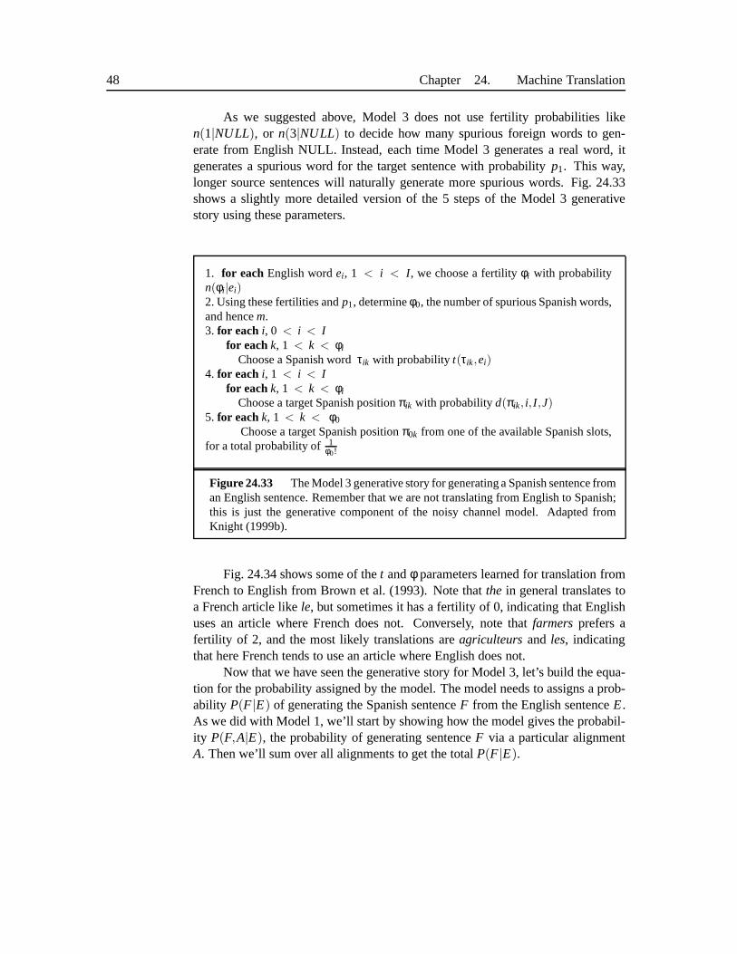
48 Chapter 24. Machine Translation
As we suggested above, Model 3 does not use fertility probabilities liken(1|NULL), or n(3|NULL) to decide how many spurious foreign words to gen-erate from English NULL. Instead, each time Model 3 generates a real word, itgenerates a spurious word for the target sentence with probability p1. This way,longer source sentences will naturally generate more spurious words. Fig. 24.33shows a slightly more detailed version of the 5 steps of the Model 3 generativestory using these parameters.
1. for each English wordei , 1 < i < I , we choose a fertilityφi with probabilityn(φi |ei)2. Using these fertilities andp1, determineφ0, the number of spurious Spanish words,and hencem.3. for each i, 0 < i < I
for eachk, 1 < k < φi
Choose a Spanish wordτik with probabilityt(τik,ei)4. for each i, 1 < i < I
for eachk, 1 < k < φi
Choose a target Spanish positionπik with probabilityd(πik, i, I ,J)5. for eachk, 1 < k < φ0
Choose a target Spanish positionπ0k from one of the available Spanish slots,for a total probability of 1
φ0!
Figure 24.33 The Model 3 generative story for generating a Spanish sentence froman English sentence. Remember that we are not translating from English to Spanish;this is just the generative component of the noisy channel model. Adapted fromKnight (1999b).
Fig. 24.34 shows some of thet andφ parameters learned for translation fromFrench to English from Brown et al. (1993). Note thatthe in general translates toa French article likele, but sometimes it has a fertility of 0, indicating that Englishuses an article where French does not. Conversely, note thatfarmersprefers afertility of 2, and the most likely translations areagriculteursand les, indicatingthat here French tends to use an article where English does not.
Now that we have seen the generative story for Model 3, let’s build the equa-tion for the probability assigned by the model. The model needs to assigns a prob-ability P(F|E) of generating the Spanish sentenceF from the English sentenceE.As we did with Model 1, we’ll start by showing how the model gives the probabil-ity P(F,A|E), the probability of generating sentenceF via a particular alignmentA. Then we’ll sum over all alignments to get the totalP(F|E).

Section 24.10. Advanced: IBM Model 3 for fertility-based alignment 49
the farmers notf t( f |e) φ n(φ|e) f t( f |e) φ n(φ|e) f t( f |e) φ n(φ|e)le 0.497 1 0.746 agriculteurs 0.442 2 0.731 ne 0.497 2 0.735la 0.207 0 0.254 les 0.418 1 0.228 pas 0.442 0 0.154les 0.155 cultivateurs 0.046 0 0.039 non 0.029 1 0.107l’ 0.086 producteurs 0.021 rien 0.011ce 0.018cette 0.011
Figure 24.34 Examples of Model 3 parameters from Brown et al. (1993), for threeEnglish words. Note that bothfarmersandnotare likely to have fertilities of 2.
In order to computeP(F,A|E), we’ll need to multiply the main three factorsn, t, andd, for generating words, translating them into Spanish, and moving themaround. So a first pass atP(F,A|E) would be:
I∏
i=1
n(φi |ei)×J∏
j=1
t( f j |eaj )×J∏
j=1
d( j|a j , I ,J)(24.37)
But (24.37) isn’t sufficient as it stands; we need to add factors for generatingspurious words, for inserting them into the available slots, and a factor having todo with the number of ways (permutations) a word can align with multiple words.Equation (24.38) gives the true final equation for IBM Model 3, in Knight’s modifi-cation of the original formula. We won’t give the details of these additional factors,but encourage the interested reader to see the original presentation in Brown et al.(1993) and the very clear explanation of the equation in Knight (1999b).
P(F,A|E) =
generate spurious︷ ︸︸ ︷(
J−φ0
φ0
)
pJ−2φ00 pφ0
1 ×
insert spurious︷︸︸︷
1φ0!
×
multi-align permutations︷ ︸︸ ︷
I∏
i=0
φi !
×I∏
i=1
n(φi |ei)×J∏
j=1
t( f j |eaj )×J∏
j:aj 6=0
d( j|a j , I ,J)(24.38)
Once again, in order to get the total probability of the Spanish sentence we’llneed to we would sum over all possible alignments:
P(F|E) =∑
A
P(F,A|E)
We can also make it more explicit exactly how we sum over alignments (andalso emphasize the incredibly large number of possible alignments) by expressingthis formula as follows, where we specify an alignment by specifying the alignedEnglisha j for each of theJ words in the foreign sentence:

50 Chapter 24. Machine Translation
P(F|E) =J∑
a1=0
J∑
a2=0
· · ·I∑
aJ=0
P(F,A|E)
24.10.1 Training for Model 3
Given a parallel corpus, training the translation model forIBM Model 3 meanssetting values for then, d, t, andp1 parameters.
As we noted for Model 1 and HMM models, if the training-corpuswas hand-labeled with perfect alignments, getting maximum likelihood estimates would besimple. Consider the probabilityn(0|did) that a word likedid would have a zerofertility. We could estimate this from an aligned corpus just by counting the num-ber of timesdid aligned to nothing, and normalize by the total count ofdid. Wecan do similar things for the thet translation probabilities. To train the distortionprobability d(1,3,6,7), we similarly count the number of times in the corpus thatEnglish worde1 maps to Spanish wordf3 in English sentences of length 6 that arealigned to Spanish sentences of length 7. Let’s call this counting function dcount.We’ll again need a normalization factor;
d(1,3,6,7) =dcount(1,3,6,7)
∑Ii=1 dcount(i,3,6,7)
(24.39)
Finally, we need to estimatep1. Again, we look at all the aligned sentences inthe corpus; let’s assume that in the Spanish sentences thereare a total ofN words.From the alignments for each sentence, we determine that a total of S Spanishwords are spurious, i.e. aligned to English NULL. ThusN−Sof the words in theSpanish sentences were generated by real English words. After S of theseN−SSpanish words, we generate a spurious word. The probabilityp1 is thusS/(N−S).
Of course, we don’t have hand-alignments for Model 3. We’ll need to useEM to learn the alignments and the probability model simultaneously. With Model1 and the HMM model, there were efficient ways to do training without explic-itly summing over all alignments. Unfortunately, this is not true for Model 3; weactually would need to compute all possible alignments. Fora real pair of sen-tences, with 20 English words and 20 Spanish words, and allowing NULL andallowing fertilities, there are a very large number of possible alignments (deter-mining the exact number of possible alignments is left as Exercise 24.7). Instead,we approximate by only considering the best few alignments.In order to find thebest alignments without looking at all alignments, we can use an iterative or boot-strapping approach. In the first step, we train the simpler IBM Model 1 or 2 asdiscussed above. Then we use these Model 2 parameters to evaluateP(A|E,F),giving a way to find the best alignments to bootstrap Model 3. See Brown et al.

Section 24.11. Other Advanced Issues in Statistical MT 51
(1993) and Knight (1999b) for details.
24.11 OTHER ADVANCED ISSUES INSTATISTICAL MT
24.11.1 Log-Linear Models
While statistical MT was first described based on the noisy channel model, it isalso possible to combine the language model and translationmodel in more so-phisticated ways than simply multiplying them. Much recentwork is based onlog-linear models, in which we directly search for the sentence with the highestposterior probability:
E = argmaxE
P(E|F)(24.40)
This is done by modelingP(E|F) via a set ofM feature functionshm(E,F), eachof which has a parameterλm. The translation probability is then:
P(E|F) =exp[
∑Mm=1λmhm(E,F)]
∑′E exp[
∑Mm=1λmhm(E′,F)]
(24.41)
The best sentence is thus:
E = argmaxE
P(E|F)
= argmaxE
exp[M∑
m=1
λmhm(E,F)](24.42)
In practice, the two factors from the noisy channel model, the language modeland translation model, are still the most important featurefunctions in the log-linear model, but the architecture has the advantage of allowing for arbitrary otherfeatures as well. See Foster (2000), Och and Ney (2002, 2004)for details.
Log-linear models for MT can be trained using the standard maximum mutualinformation criterion. In more recent systems, however, the log-linear models areinstead trained to directly optimize evaluation metrics like Bleu (Och, 2003).
24.11.2 Syntactic Models
Modern statistical MT systems are no longer based on words asthe elementaryunits, since phrase-based models for statistical MT produce consistently better re-sults. The phrase-based models we have described above are not constrained tomatch the syntactic boundaries assigned by traditional parsers. Indeed, early ex-periments in applying syntax to MT suggested that induced phrases worked betterthan traditional parse constituents.
52 Chapter 24. Machine Translation
More recent research, however, suggests that syntactic knowledge, whetherin the form of dependency structures, hierarchical phrase models, or traditionalparse structures, does seem to improve MT performance.
One promising class of approaches assigns a parallel syntactic tree structureto a pair of sentences in different languages, with the goal of translating the sen-tences by applying reordering operations on the trees. The mathematical model forthese parallel structures issynchronous grammar. A synchronous grammar (alsoSYNCHRONOUS
GRAMMAR
called atransduction grammar) is a structurally correlated pair of languages; weTRANSDUCTIONGRAMMAR
can view such as grammar as generating pairs of aligned sentences in two lan-guages. A synchronous Context-Free Grammar, for example, is a kind of syn-chronous grammar that allow us to represent and parse context-free grammars overpairs of sentences (Wu, 1997). One of the earliest such models for MT wasinver-sion transduction grammars (ITG), a subset of synchronous context-free gram-INVERSION
TRANSDUCTIONGRAMMARS
mars. Inversion transduction grammars are binary synchronous CFGs; the intuitionis that individual binary rules for one of the sentence pairsto be generated in re-verse order, allowing us to capture word-order differencesin the two languages.Lexicalized version of ITGs also exist (Zhang and Gildea, 2005).
More general synchronous Context-Free Grammars have also been used. Thesystem of Chiang (2005), for example, uses synchronous CFGsto learn hierarchi-cal phrases. His model learns hierarchical pairs of rules that capture the fact thatChinese relative clauses appear to the left of their head, while English relativeclauses appear to the right of their head:
<① de②, the② that①>
Other models for translation by aligning parallel parse trees including (Ya-mada and Knight, 2001; ?; Melamed, 2003; ?, ?, ?).
BIBLIOGRAPHICAL AND HISTORICAL NOTES
Work on models of the process and goals of translation goes back at least to SaintJerome in the fourth century (Kelley, 1979). The development of logical languages,free of the imperfections of human languages, for reasoningcorrectly and for com-municating truths and thereby also for translation, has been pursued at least sincethe 1600s (Hutchins, 1986).
By the late 1940s, scant years after the birth of the electronic computer, theidea of MT was raised seriously (Weaver, 1955). In 1954 the first public demonstra-tion of a MT system prototype (Dostert, 1955) led to great excitement in the press(Hutchins, 1997). The next decade saw a great flowering of ideas, prefiguring mostsubsequent developments. But this work was ahead of its time— implementations

Section 24.11. Other Advanced Issues in Statistical MT 53
were limited by, for example, the fact that pending the development of disks therewas no good way to store dictionary information.
As high quality MT proved elusive (Bar-Hillel, 1960), a growing consensuson the need for better evaluation and more basic research in the new fields of formaland computational linguistics, culminating in the famous ALPAC (Automatic Lan-guage Processing Advisory Committee) report of 1966 (Pierce et al., 1966), led inthe mid 1960s to a dramatic cut in funding for MT. As MT research lost academicrespectability, the Association for Machine Translation and Computational Lin-guistics dropped MT from its name. Some MT developers, however, persevered,slowly and steadily improving their systems, and slowly garnering more customers.Systran in particular, developed initially by Peter Toma, has been continuouslyimproved over 40 years. Its earliest uses were for information acquisition, forexample by the U.S. Air Force for Russian documents; and in 1976 an English-French edition was adopted by the European Community for creating rough andpost-editable translations of various administrative documents. Another early suc-cessful MT system was Meteo, which translated weather forecasts from Englishto French; incidentally, its original implementation (1976), used “Q-systems”, anearly unification model.
The late 1970s saw the birth of another wave of academic interest in MT.One strand attempted to apply meaning-based techniques developed for story un-derstanding and knowledge engineering (Carbonell et al., 1981). There were widediscussions of interlingual ideas through the late 1980s and early 1990s (Tsujii,1986; Nirenburg et al., 1992; Ward, 1994; Carbonell et al., 1992) Meanwhile MTusage was increasing, fueled by globalization, governmentpolicies requiring thetranslation of all documents into multiple official languages, and the proliferationof word processors and then personal computers.
Modern statistical methods began to be applied in the early 1990s, enabledby the development of large bilingual corpora and the growthof the web. Early on,a number of researchers showed that it was possible to extract pairs of aligned sen-tences from bilingual corpora (Kay and Roscheisen, 1988; ?; Brown et al., 1991;Gale and Church, 1991, 1993; Kay and Roscheisen, 1993). Theearliest algorithmsmade use of the words of the sentence as part of the alignment model, while othersrelied solely on other cues like sentence length in words or characters.
At the same time, the IBM group, drawing directly on algorithms for speechrecognition (many of which had themselves been developed originally at IBM!)proposed theCandide system, based on the IBM statistical models we have de-CANDIDE
scribed (Brown et al., 1990, 1993). These papers described the probabilistic modeland the parameter estimation procedure. The decoding algorithm was never pub-lished, but it was described in a patent filing (Brown et al., 1995). The IBM workhad a huge impact on the research community, and by the turn ofthis century,
54 Chapter 24. Machine Translation
much or most academic research on machine translation was statistical. Progresswas made hugely easier by the development of publicly-available toolkits, partic-ularly tools extended from theEGYPT toolkit developed by the Statistical Ma-EGYPT
chine Translation team in during the summer 1999 research workshop at the Cen-ter for Language and Speech Processing at the Johns Hopkins University. Theseinclude theGIZA++ aligner, developed by Franz Joseph Och by extending theGIZA++
GIZA toolkit (Och and Ney, 2003), which implements IBM models 1-5 as well asthe HMM alignment model.
Initially most research implementations focused on IBM Model 3, but veryquickly researchers moved to phrase-based models. While the earliest phrase-based translation model was IBM Model 4 (Brown et al., 1993),modern modelsderive from Och’s (?) work onalignment templates. Key phrase-based translationmodels include Marcu and Wong (2002), Yamada and Knight (2001), ? (?). Venu-gopal et al. (2003), Koehn et al. (2003), ? (?) Och and Ney (2004), Deng and Byrne(2005), and Kumar and Byrne (2005), A further extension to the EGYPT tools dis-cussed above is a publicly available phrase-based stack decoder,PHARAOH , de-PHARAOH
veloped by Philipp Koehn (Koehn, 2004, 2003b), which extended theA∗ decodersof (Och et al., 2001) and Brown et al. (1995). Other work on MT decoding includesthe A∗ decoders of Wang and Waibel (1997) and Germann et al. (2001),and thepolynomial-time decoder for binary-branching stochastictransduction grammar ofWu (1996).
Modern research continues on sentence and word alignment aswell; morerecent algorithms include ? (?, ?, ?, ?, ?).
Research on evaluation of machine translation began quite early. Miller andBeebe-Center (1958) proposed a number of methods drawing onwork in psy-cholinguistics. These included the use of cloze and Shannontasks to measureintelligibility, as well as a metric of edit distance from a human translation, theintuition that underlies all modern automatic evaluation metrics like Bleu. TheALPAC report included an early evaluation study conducted by John Carroll thatwas extremely influential (Pierce et al., 1966, Appendix 10). Carroll proposeddistinct measures for fidelity and intelligibility, and hadspecially trained humanraters score them subjectively on 9-point scales. More recent work on evaluationhas focused on coming up with automatic metrics, include thework on Bleu dis-cussed in Sec. 24.9.2 (Papineni et al., 2002), as well as related measures likeNIST(Doddington, 2002),Precision and Recall(Turian et al., 2003), andMETEOR(Banerjee and Lavie, 2005).
Good surveys of the early history of MT are Hutchins (1986) and (1997).The textbook by Hutchins and Somers (1992) includes a wealthof examples oflanguage phenomena that make translation difficult, and extensive descriptions ofsome historically significant MT systems. Nirenburg et al. (2002) is a comprehen-

Section 24.11. Other Advanced Issues in Statistical MT 55
sive collection of classic readings in MT. (Knight, 1999b) is an excellent tutorialintroduction to Statistical MT.
Academic papers on machine translation appear in standard NLP journals andconferences, as well as in the journalMachine Translationand in the proceedingsof various conferences, including MT Summit, organized by the International As-sociation for Machine Translation, the individual conferences of its three regionaldivisions, (Association for MT in the Americas – AMTA, European Association forMT – EAMT, and Asia-Pacific Association for MT – AAMT), and theConferenceon Theoretical and Methodological Issue in Machine Translation (TMI).
EXERCISES
24.1 Select at random a paragraph of Ch. 11 which describes a fact about Englishsyntax. a) Describe and illustrate how your favorite foreign language differs in thisrespect. b) Explain how a MT system could deal with this difference.
24.2 Choose a foreign language novel in a language you know. Copy down theshortest sentence on the first page. Now look up the renditionof that sentence inan English translation of the novel. a) For both original andtranslation, draw parsetrees. b) For both original and translation, draw dependency structures. c) Drawa case structure representation of the meaning which the original and translationshare. d) What does this exercise suggest to you regarding intermediate represen-tations for MT?
24.3 Version 1 (for native English speakers): Consider the following sentence:
These lies are like their father that begets them; gross as a mountain, open,palpable.
Henry IV, Part 1, act 2, scene 2
Translate this sentence into some dialect of modern vernacular English. Forexample, you might translate it into the style of a New York Times editorial oran Economist opinion piece, or into the style of your favorite television talk-showhost.
Version 2 (for native speakers of other languages): Translate the followingsentence into your native language.
One night my friend Tom, who had just moved into a new apartment, saw acockroach scurrying about in the kitchen.
For either version, now:
56 Chapter 24. Machine Translation
a) Describe how you did the translation: What steps did you perform? Inwhat order did you do them? Which steps took the most time? b) Could you writea program that would translate using the same methods that you did? Why or whynot? c) What aspects were hardest for you? Would they be hard for a MT system?d) What aspects would be hardest for a MT system? are they hardfor people too?e) Which models are best for describing various aspects of your process (direct,transfer, interlingua or statistical)? f) Now compare yourtranslation with thoseproduced by friends or classmates. What is different? Why were the translationsdifferent?
24.4 Type a sentence into a MT system (perhaps a free demo on the web) and seewhat it outputs. a) List the problems with the translation. b) Rank these problemsin order of severity. c) For the two most severe problems, suggest the probable rootcause.
24.5 Build a very simple direct MT system for translating from some languageyou know at least somewhat into English (or into a language inwhich you arerelatively fluent), as follows. First, find some good test sentences in the sourcelanguage. Reserve half of these as a Next, acquire a bilingual dictionary for thesetwo languages (for many languages, limited dictionaries can be found on the webthat will be sufficient for this exercise). Your program should translate each wordby looking up its translation in your dictionary. You may need to implement somestemming or simple morphological analysis. Next, examine your output, and doa preliminary error analysis. What are the major sources of error? Write somegeneral rules for correcting the translation mistakes. Youwill probably want to runa part-of-speech tagger on the English output, if you have one.
24.6 Continue the calculations for the EM example on page 33, performing thesecond and third round of E-steps and M-steps.
24.7 (Derived from Knight (1999b)) How many possible Model 3 alignmentsare there between a 20-word English sentence and a 20-word Spanish sentence,allowing for NULL and fertilities?
Section 24.11. Other Advanced Issues in Statistical MT 57
Banerjee, S. and Lavie, A. (2005). METEOR: An auto-matic metric for Mt evaluation with improved correlationwith human judgments. InProceedings of ACL Work-shop on Intrinsic and Extrinsic Evaluation Measures forMT and/or Summarization.
Bar-Hillel, Y. (1960). The present status of automatictranslation of languages. In Alt, F. (Ed.),Advances inComputers 1, pp. 91–163. Academic Press.
Bickel, B. (2003). Referential density in discourse andsyntactic typology.Language, 79(2), 708–736.
Brown, P., Cocke, J., Pietra, S. D., Pietra, V. D., Jelinek,F., Lai, J., and Mercer, R. (1995). Method and system fornatural language translation. U.S. Patent 5,477,451.
Brown, P. F., Cocke, J., Della Pietra, S. A., Della Pietra,V. J., Jelinek, F., Lafferty, J. D., Mercer, R. L., andRoossin, P. S. (1990). A statistical approach to machinetranslation.Computational Linguistics, 16(2), 79–85.
Brown, P. F., Della Pietra, S. A., Della Pietra, V. J., andMercer, R. L. (1993). The mathematics of statistical ma-chine translation: Parameter estimation.ComputationalLinguistics, 19(2), 263–311.
Brown, P. F., Lai, J. C., and Mercer, R. L. (1991). Aligningsentences in parallel corpora. InProceedings of the 29thACL, Berkeley, CA, pp. 169–176. ACL.
Callison-Burch, C., Osborne, M., and Koehn, P. (2006).Re-evaluating the role of BLEU in machine translationresearch. InEACL-06.
Cao, X. (1792). The Story of the Stone.(Also known asThe Dream of the Red Chamber). Penguin Classics, Lon-don. First published in Chinese in 1792, translated intoEnglish by David Hawkes and published by Penguin in1973.
Carbonell, J., Cullingford, R. E., and Gershman, A. V.(1981). Steps toward knowledge-based machine trans-lation. IEEE Transactions on Pattern Analysis and Ma-chine Intelligence, 3(4), 376–392.
Carbonell, J., Mitamura, T., and Nyberg, E. H. (1992). TheKANT perspective: A critique of pure transfer (and pureinterlingua, pure statistics, ...). InInternational Confer-ence on Theoretical and Methodological Issues in Ma-chine Translation.
Chandioux, J. (1976). METEO: un systemeoperationnel pour la traduction automatique des bul-letins meteorologiques destines au grand public.Meta,21, 127–133.
Chiang, D. (2005). A hierarchical phrase-based model forstatistical machine translation. InProceedings of ACL-05, Ann Arbor, MI, pp. 263–270. ACL.
Comrie, B. (1989).Language Universals and LinguisticTypology. Basil Blackwell, Oxford. Second edition.
Croft, W. (1990). Typology and Universals. CambridgeUniversity Press, Cambridge.
Deng, Y. and Byrne, W. (2005). Hmm word and phrasealignment for statistical machine translation. InProceed-ings of HLT-EMNLP-05.
Doddington, G. (2002). Automatic evaluation of machinetranslation quality using n-gram co-occurrence statistics.In Proceedings of HLT-02.
Dostert, L. (1955). The Georgetown-I.B.M. experiment.In Machine Translation of Languages: Fourteen Essays,pp. 124–135. MIT Press.
Foster, G. (2000). A maximum entropy/minimum diver-gence translation model. InProceedings of ACL-00,Hong Kong. ACL.
Gale, W. A. and Church, K. W. (1991). A program foraligning sentences in bilingual corpora. InProceedingsof the 29th ACL, Berkeley, CA, pp. 177–184. ACL.
Gale, W. A. and Church, K. W. (1993). A program foraligning sentences in bilingual corpora.ComputationalLinguistics, 19, 75–102.
Germann, U., Jahr, M., Knight, K., Marcu, D., and Ya-mada, K. (2001). Fast decoding and optimal decodingfor machine translation. InProceedings of ACL-01, pp.228–235. ACL.
Hutchins, J. (1997). From first conception to first demon-stration: the nascent years of machine translation, 1947–1954. A chronology.Machine Translation, 12, 192–252.
Hutchins, W. J. and Somers, H. L. (1992).An Introductionto Machine Translation. Academic Press.
Hutchins, W. J. (1986). Machine Translation: Past,Present, Future. Ellis Horwood, Chichester, England.
Jelinek, F. (1969). A fast sequential decoding algorithmusing a stack. IBM Journal of Research and Develop-ment, 13, 675–685.
Kay, M. and Roscheisen, M. (1988). Text-translationalignment. Tech. rep. P90-00143, Xerox Palo Alto Re-search Center, Palo Alto, CA.
Kay, M. and Roscheisen, M. (1993). Text-translationalignment.Computational Linguistics, 19, 121–142.

58 Chapter 24. Machine Translation
Kelley, L. G. (1979). The True Interpreter: A History ofTranslation Theory and Practice in the West. St. Martin’sPress, New York.
Knight, K. (1999a). Decoding complexity in word-replacement translation models.Computational Linguis-tics, 25(4), 607–615.
Knight, K. (1999b). A statistical MT tutorial workbook..
Koehn, P. (2003a).Noun Phrase Translation. Ph.D. thesis,University of Southern California.
Koehn, P. (2003b). Pharaoh: a beam search decoderfor phrase-based statistical machine translation models:User manual and description..
Koehn, P. (2004). Pharaoh: a beam search decoder forphrase-based statistical machine translation models. InProceedings of AMTA 2004.
Koehn, P., Och, F. J., and Marcu, D. (2003). Statisti-cal phrase-based translation. InProceedings of HLT-NAACL-03, pp. 48–54.
Kumar, S. and Byrne, W. (2005). Local phrase reorderingmodels for statistical machine translation. InProceed-ings of HLT-EMNLP-05.
Levin, L., Gates, D., Lavie, A., and Waibel, A. (1998). Aninterlingua based on domain actions for machine trans-lation of task-oriented dialogues. InICSLP-98, Sydney,pp. 1155–1158.
Li, C. N. and Thompson, S. A. (1981).Mandarin Chi-nese: A Functional Reference Grammar. University ofCalifornia Press.
Marcu, D. and Wong, W. (2002). A phrase-based, jointprobability model for statistical machine translation. InEMNLP 2002, pp. 133–139. ACL.
McLuhan, M. (1964).Understanding media: The exten-sions of man. New American Library, New York.
Melamed, I. D. (2003). Multitext grammars and syn-chronous parsers. InProceedings of HLT-NAACL-03.ACL.
Miller, G. A. and Beebe-Center, J. G. (1958). Some psy-chological methods for evaluating the quality of transla-tions. Mechanical Translation, 3, 73–80.
Nichols, J. (1986). Head-marking and dependent-markinggrammar.Language, 62(1), 56–119.
Nirenburg, S., Carbonell, J., Tomita, M., and Goodman,K. (1992). Machine Translation: A Knowledge-basedApproach. Morgan Kaufmann.
Nirenburg, S., Somers, H. L., and Wilks, Y. A. (Eds.).(2002). Readings in Machine Translation. MIT Press,Cambridge, MA.
Och, F. J. (2003). Minimum error rate training in statisti-cal machine translation. InProceedings of ACL-03, pp.160–167.
Och, F. J. and Ney, H. (2002). Discriminative training andmaximum entropy models for statistical machine transla-tion. In Proceedings of ACL-02, pp. 295–302. ACL.
Och, F. J. and Ney, H. (2003). A systematic comparisonof various statistical alignment models.ComputationalLinguistics, 29(1), 19–51.
Och, F. J. and Ney, H. (2004). The alignment template ap-proach to statistical machine translation.ComputationalLinguistics, 30(4), 417–449.
Och, F. J., Ueffing, N., and Ney, H. (2001). An efficienta* search algorithm for statistical machine translation. InProceedings of the ACL Workshop on Data-Driven meth-ods in Machine Translation, pp. 1–8. ACL.
Papineni, K., Roukos, S., Ward, T., and Zhu, W.-J. (2002).Bleu: a method for automatic evaluation of machinetranslation. InProceedings of ACL-02, Philadelphia, PA.
Pierce, J. R., Carroll, J. B., and et al (1966).Languageand Machines: Computers in Translation and Linguis-tics. ALPAC report. National Academy of Sciences, Na-tional Research Council, Washington, DC.
Slobin, D. I. (1996). Two ways to travel. In Shibatani,M. and Thompson, S. A. (Eds.),Grammatical Construc-tions: Their Form and Meaning, pp. 195–220. ClarendonPress, Oxford.
Talmy, L. (1985). Lexicalization patterns: Semantic struc-ture in lexical forms. In Shopen, T. (Ed.),Language Ty-pology and Syntactic Description, Volume 3. CambridgeUniversity Press. Originally appeared as UC BerkeleyCognitive Science Program Report No. 30, 1980.
Talmy, L. (1991). Path to realization: a typology of eventconflation. InBLS-91, Berkeley, CA, pp. 480–519.
Toutanova, K., Ilhan, H. T., and Manning, C. D. (2002).Extensions to HMM-based statistical word alignmentmodels., 87–94.
Tsujii, J. (1986). Future directions of machine translation.In COLING-86, Bonn, pp. 655–668.
Turian, J. P., Shen, L., and Melamed, I. D. (2003). Eval-uation of machine translation and its evaluation. InPro-ceedings of MT Summit IX, New Orleans, LA.
Section 24.11. Other Advanced Issues in Statistical MT 59
Venugopal, A., Vogel, S., and Waibel, A. (2003). Effectivephrase translation extraction from alignment models. InProceedings of ACL-03, pp. 319–326. ACL.
Wang, Y. and Waibel, A. (1997). Decoding algorithmin statistical machine translation. InACL/EACL-97, pp.366–372. ACL.
Ward, N. (1994). A Connectionist Language Generator.Ablex.
Waugh, L. R. (1976). The semantics and paradigmatics ofword order.Language, 52(1), 82–107.
Weaver, W. (1949/1955). Translation. In Locke, W. N. andBoothe, A. D. (Eds.),Machine Translation of Languages,pp. 15–23. MIT Press, Cambridge, MA. Reprinted froma memorandum written by Weaver in 1949.
Wu, D. (1996). A polynomial-time algorithm for statisti-cal machine translation. InProceedings of ACL-96, SantaCruz, CA, pp. 152–158. ACL.
Wu, D. (1997). Stochastic inversion transduction gram-mars and bilingual parsing of parallel corpora.Compu-tational Linguistics, 23(3), 3–403.
Yamada, K. and Knight, K. (2001). A syntax-based sta-tistical translation model. InProceedings of ACL-01,Toulouse, France.
Yamada, K. and Knight, K. (2002). A decoder forsyntax-based statistical MT. InProceedings of ACL-02,Philadelphia, PA.
Zhang, H. and Gildea, D. (2005). Stochastic lexicalizedinversion transduction grammar for alignment. InPro-ceedings of ACL-05, Ann Arbor, MI. ACL.