22BBook.pdf

7/27/2019 22BBook.pdf

http://slidepdf.com/reader/full/22bbookpdf 1/133

Lectures on Differential Equations1

Craig A. Tracy2

Department of MathematicsUniversity of California

Davis, CA 95616

November 2012

1 c Craig A. Tracy, 2000, 2012 Davis, CA 956162email: [email protected]

7/27/2019 22BBook.pdf


2

7/27/2019 22BBook.pdf


Contents

1 Pendulum and MatLab 1

1.1 Differential Equations . . . . . . . . . . . . . . . . . . . . . . . . . . . . . . . 2

1.2 Introduction to Computer Software . . . . . . . . . . . . . . . . . . . . . . . . 4

1.3 Exercises . . . . . . . . . . . . . . . . . . . . . . . . . . . . . . . . . . . . . . 8

2 First Order Equations 11

2.1 Linear First Order Equations . . . . . . . . . . . . . . . . . . . . . . . . . . . 11

2.2 Separation of Variables Applied to Mechanics . . . . . . . . . . . . . . . . . . 16

2.3 Exercises . . . . . . . . . . . . . . . . . . . . . . . . . . . . . . . . . . . . . . 25

3 Second Order Linear Equations 33

3.1 Theory of Second Order Equations . . . . . . . . . . . . . . . . . . . . . . . . 34

3.2 Reduction of Order . . . . . . . . . . . . . . . . . . . . . . . . . . . . . . . . . 37

3.3 Constant Coefficients . . . . . . . . . . . . . . . . . . . . . . . . . . . . . . . . 38

3.4 Forced Oscillations of the Mass-Spring System . . . . . . . . . . . . . . . . . 43

3.5 Exercises . . . . . . . . . . . . . . . . . . . . . . . . . . . . . . . . . . . . . . 47

4 Difference Equations 51

4.1 Introduction . . . . . . . . . . . . . . . . . . . . . . . . . . . . . . . . . . . . . 52

4.2 Constant Coefficient Difference Equations . . . . . . . . . . . . . . . . . . . . 52

4.3 Inhomogeneous Difference Equations . . . . . . . . . . . . . . . . . . . . . . . 54

4.4 Exercises . . . . . . . . . . . . . . . . . . . . . . . . . . . . . . . . . . . . . . 54

i

7/27/2019 22BBook.pdf


ii CONTENTS

5 Matrix Differential Equations 57

5.1 The Matrix Exponential . . . . . . . . . . . . . . . . . . . . . . . . . . . . . . 58

5.2 Application of Matrix Exponential to DEs . . . . . . . . . . . . . . . . . . . . 60

5.3 Relation to Earlier Methods of Solving Constant Coefficient DEs . . . . . . . 63

5.4 Inhomogenous Matrix Equations . . . . . . . . . . . . . . . . . . . . . . . . . 63

5.5 Exercises . . . . . . . . . . . . . . . . . . . . . . . . . . . . . . . . . . . . . . 64

6 Weighted String 69

6.1 Derivation of Differential Equations . . . . . . . . . . . . . . . . . . . . . . . . 70

6.2 Reduction to an Eigenvalue Problem . . . . . . . . . . . . . . . . . . . . . . . 72

6.3 Computation of the Eigenvalues . . . . . . . . . . . . . . . . . . . . . . . . . . 73

6.4 The Eigenvectors . . . . . . . . . . . . . . . . . . . . . . . . . . . . . . . . . . 76

6.5 Determination of constants . . . . . . . . . . . . . . . . . . . . . . . . . . . . 77

6.6 Continuum Limit: The Wave Equation . . . . . . . . . . . . . . . . . . . . . . 81

6.7 Inhomogeneous Problem . . . . . . . . . . . . . . . . . . . . . . . . . . . . . . 84

6.8 Vibrating Membrane . . . . . . . . . . . . . . . . . . . . . . . . . . . . . . . . 85

6.9 Exercises . . . . . . . . . . . . . . . . . . . . . . . . . . . . . . . . . . . . . . 90

7 Quantum Harmonic Oscillator 99

7.1 Schrodinger Equation . . . . . . . . . . . . . . . . . . . . . . . . . . . . . . . 100

7.2 Harmonic Oscillator . . . . . . . . . . . . . . . . . . . . . . . . . . . . . . . . 101

7.3 Some properties of the harmonic oscillator . . . . . . . . . . . . . . . . . . . . 109

7.4 The Heisenberg Uncertainty Principle . . . . . . . . . . . . . . . . . . . . . . 113

7.5 Exercises . . . . . . . . . . . . . . . . . . . . . . . . . . . . . . . . . . . . . . 115

8 Laplace Transform 117

8.1 Matrix version . . . . . . . . . . . . . . . . . . . . . . . . . . . . . . . . . . . 117

8.2 Structure of (sI n − A)−1 . . . . . . . . . . . . . . . . . . . . . . . . . . . . . . 121

8.3 Exercises . . . . . . . . . . . . . . . . . . . . . . . . . . . . . . . . . . . . . . 122

7/27/2019 22BBook.pdf


CONTENTS iii

Preface

These notes are for a one-quarter course in differential equations. The approach is to tiethe study of differential equations to specific applications in physics with an emphasis onoscillatory systems. Typically I do not cover the last section on Laplace transforms butit is included as a future reference for the engineers who will need this material. I thankEunghyun (Hyun) Lee for his help with these notes during the 2008–09 academic year.

As a preface to the study of differential equations one can do no better than to quoteV. I. Arnold, Geometrical Methods in the Theory of Ordinary Differential Equations :

Newton’s fundamental discovery, the one which he considered necessary to keepsecret and published only in the form of an anagram, consists of the following:Data aequatione quotcunque fluentes quantitae involvente fluxions invenire et

vice versa . In contemporary mathematical language, this means: “It is useful to

solve differential equations”.

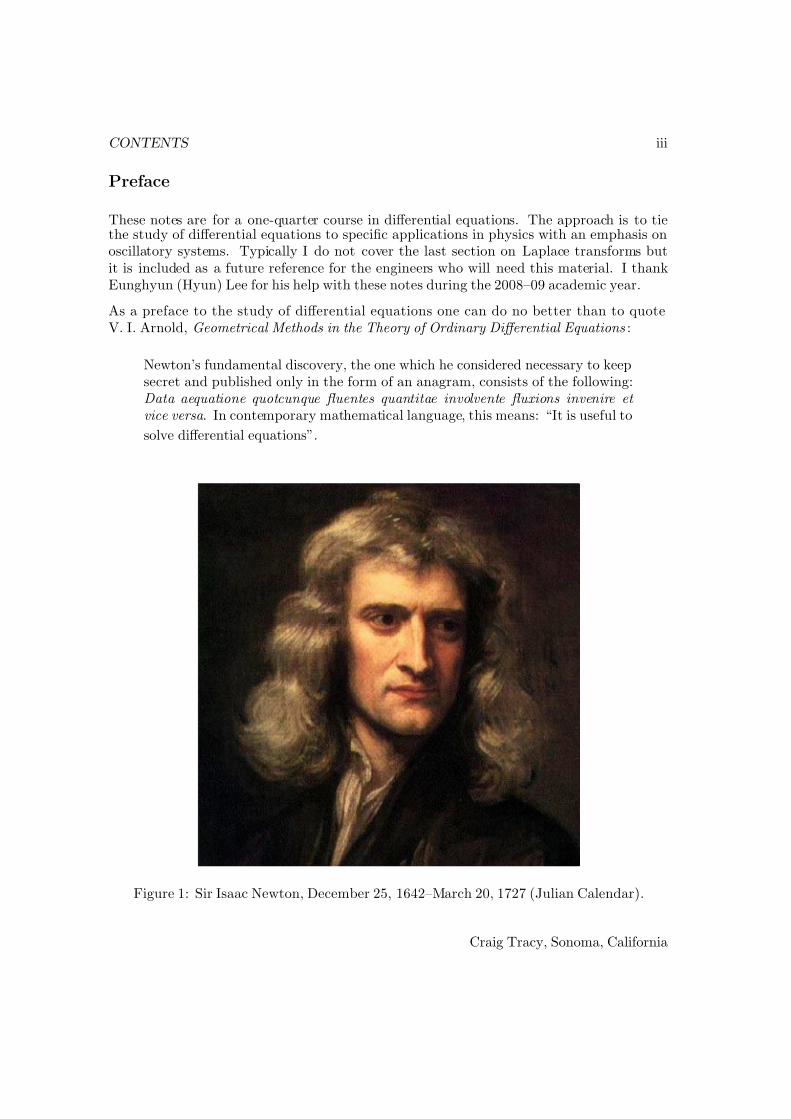
Figure 1: Sir Isaac Newton, December 25, 1642–March 20, 1727 (Julian Calendar).

Craig Tracy, Sonoma, California

7/27/2019 22BBook.pdf


iv CONTENTS

Notation

Symbol Definition of Symbol

R field of real numbersR

n the n-dimensional vector space with each component a real numberC field of complex numbersx the derivative dx/dt, t is interpreted as timex the second derivative d2x/dt2, t is interpreted as time:= equals by definitionΨ = Ψ(x, t) wave function in quantum mechanicsODE ordinary differential equationPDE partial differential equationKE kinetic energyPE potential energy

det determinantδ ij the Kronecker delta, equal to 1 if i = j and 0 otherwiseL the Laplace transform operatornk

The binomial coefficient n choose k.

Maple is a registered trademark of Maplesoft.Mathematica is a registered trademark of Wolfram Research.MatLab is a registered trademark of the MathWorks, Inc.

7/27/2019 22BBook.pdf


Chapter 1

Mathematical Pendulum

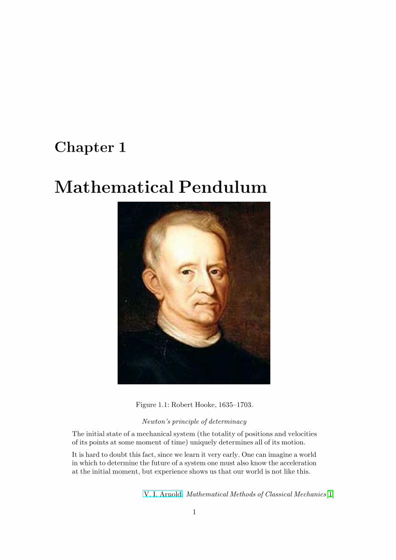
Figure 1.1: Robert Hooke, 1635–1703.

Newton’s principle of determinacy

The initial state of a mechanical system (the totality of positions and velocitiesof its points at some moment of time) uniquely determines all of its motion.

It is hard to doubt this fact, since we learn it very early. One can imagine a worldin which to determine the future of a system one must also know the accelerationat the initial moment, but experience shows us that our world is not like this.

V. I. Arnold, Mathematical Methods of Classical Mechanics [1]

1

http://en.wikipedia.org/wiki/Vladimir_Arnold

http://en.wikipedia.org/wiki/Vladimir_Arnold

7/27/2019 22BBook.pdf


2 CHAPTER 1. PENDULUM AND MATLAB

1.1 Derivation of the Differential Equations

Many interesting ordinary differential equations (ODEs) arise from applications. One reasonfor understanding these applications in a mathematics class is that you can combine yourphysical intuition with your mathematical intuition in the same problem. Usually the resultis an improvement of both. One such application is the motion of pendulum, i.e. a ballof mass m suspended from an ideal rigid rod that is fixed at one end. The problem isto describe the motion of the mass point in a constant gravitational field. Since this is amathematics class we will not normally be interested in deriving the ODE from physicalprinciples; rather, we will simply write down various differential equations and claim thatthey are “interesting.” However, to give you the flavor of such derivations (which you will seerepeatedly in your science and engineering courses), we will derive from Newton’s equationsthe differential equation that describes the time evolution of the angle of deflection of thependulum.

Let

ℓ = length of the rod measured, say, in meters,

m = mass of the ball measured, say, in kilograms,

g = acceleration due to gravity = 9.8070 m/s2.

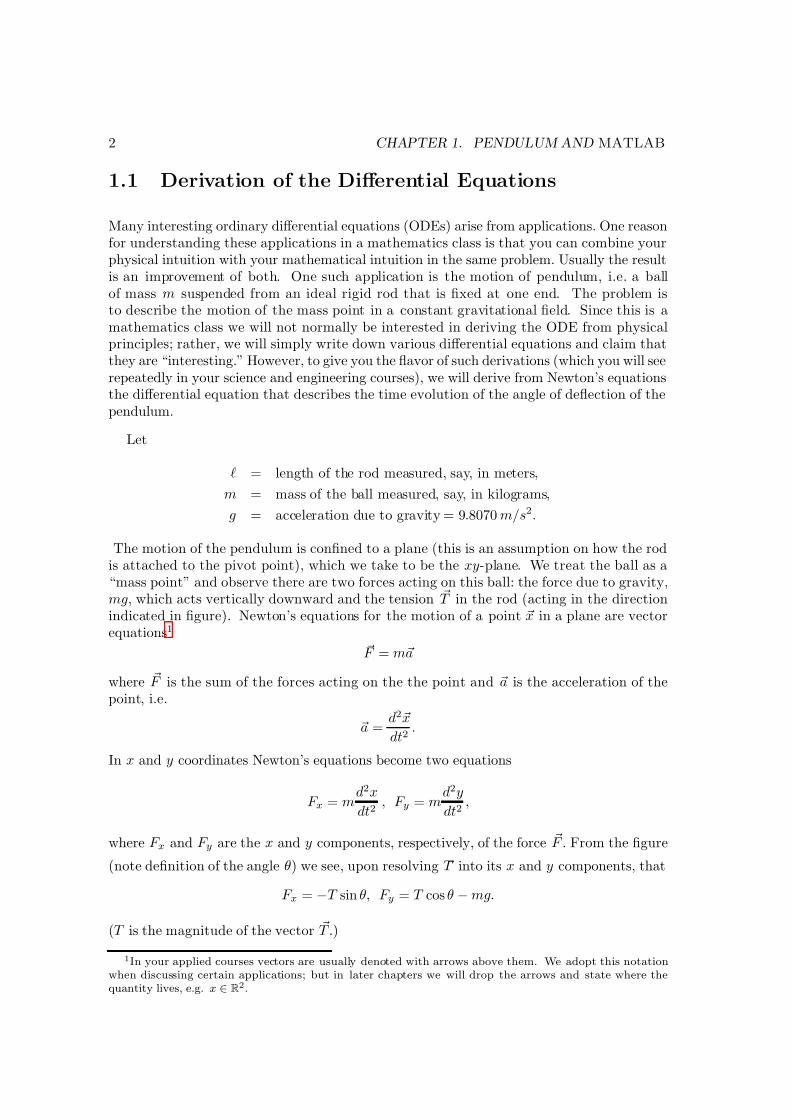
The motion of the pendulum is confined to a plane (this is an assumption on how the rodis attached to the pivot point), which we take to be the xy-plane. We treat the ball as a“mass point” and observe there are two forces acting on this ball: the force due to gravity,mg, which acts vertically downward and the tension T in the rod (acting in the directionindicated in figure). Newton’s equations for the motion of a point x in a plane are vectorequations1

F = ma

where F is the sum of the forces acting on the the point and a is the acceleration of thepoint, i.e.

a =d2x

dt2.

In x and y coordinates Newton’s equations become two equations

F x = md2x

dt2, F y = m

d2y

dt2,

where F x and F y are the x and y components, respectively, of the force F . From the figure

(note definition of the angle θ) we see, upon resolving T into its x and y components, that

F x = −T sin θ, F y = T cos θ − mg.

(T is the magnitude of the vector T .)

1In your applied courses vectors are usually denoted with arrows above them. We adopt this notationwhen discussing certain applications; but in later chapters we will drop the arrows and state where thequantity lives, e.g. x ∈ R

2.

7/27/2019 22BBook.pdf


1.1. DIFFERENTIAL EQUATIONS 3

ℓ

mass m

mg

T

θ

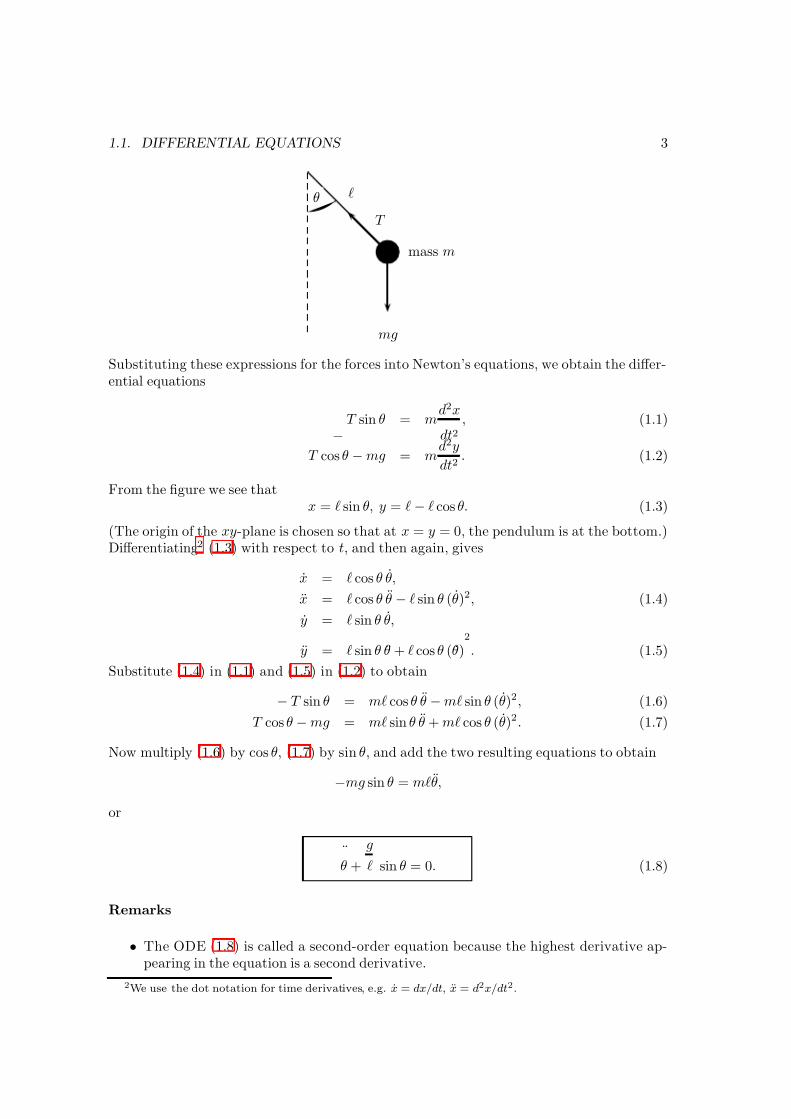
Substituting these expressions for the forces into Newton’s equations, we obtain the differ-ential equations

−T sin θ = m

d2x

dt2, (1.1)

T cos θ − mg = md2y

dt2. (1.2)

From the figure we see thatx = ℓ sin θ, y = ℓ − ℓ cos θ. (1.3)

(The origin of the xy-plane is chosen so that at x = y = 0, the pendulum is at the bottom.)Differentiating2 (1.3) with respect to t, and then again, gives

x = ℓ cos θ θ,

x = ℓ cos θ θ − ℓ sin θ (θ)2, (1.4)

y = ℓ sin θ θ,

y = ℓ sin θ θ + ℓ cos θ (θ)2

. (1.5)

Substitute (1.4) in (1.1) and (1.5) in (1.2) to obtain

− T sin θ = mℓ cos θ θ − mℓ sin θ (θ)2, (1.6)

T cos θ − mg = mℓ sin θ θ + mℓ cos θ (θ)2. (1.7)

Now multiply (1.6) by cos θ, (1.7) by sin θ, and add the two resulting equations to obtain

−mg sin θ = mℓθ,

or

¨θ +

g

ℓ sin θ = 0. (1.8)

Remarks

• The ODE (1.8) is called a second-order equation because the highest derivative ap-pearing in the equation is a second derivative.

2We use the dot notation for time derivatives, e.g. x = dx/dt, x = d2x/dt2.

7/27/2019 22BBook.pdf



• The ODE is nonlinear because of the term sin θ (this is not a linear function of theunknown quantity θ).

• A solution to this ODE is a function θ = θ(t) such that when it is substituted into theODE, the ODE is satisfied for all t.

• Observe that the mass m dropped out of the final equation. This says the motion willbe independent of the mass of the ball.

• The derivation was constructed so that the tension, T , was eliminated from the equa-tions. We could do this because we started with two unknowns, T and θ, and twoequations. We manipulated the equations so that in the end we had one equation forthe unknown θ = θ(t).

•We have not discussed how the pendulum is initially started. This is very important

and such conditions are called the initial conditions .

We will return to this ODE later in the course. At this point we note that if we wereinterested in only small deflections from the origin (this means we would have to start outnear the origin), there is an obvious approximation to make. Recall from calculus the Taylorexpansion of sin θ

sin θ = θ − θ3

3!+

θ5

5!+ · · · .

For small θ this leads to the approximation sin θ ≈ θ . Using this small deflection approxi-mation in (1.8) leads to the ODE

θ +g

ℓθ = 0. (1.9)

We will see that (1.9) is mathematically simpler than (1.8). The reason for this is that (1.9)is a linear ODE. It is linear because the unknown quantity, θ, and its derivatives appearonly to the first or zeroth power.

1.2 Introduction to MatLab, Mathematica and Maple

In this class we may use the computer software packages MatLab, Mathematica or Maple

to do routine calculations. It is strongly recommended that you learn to use at least one of these software packages. These software packages take the drudgery out of routine calcula-tions in calculus and linear algebra. Engineers will find that MatLab is used extenstivelyin their upper division classes. Both MatLab and Maple are superior for symbolic compu-tations (though MatLab can call Maple from the MatLab interface).

7/27/2019 22BBook.pdf


1.2. INTRODUCTION TO COMPUTER SOFTWARE 5

1.2.1 MatLab

What is MatLab ? “MatLab is a powerful computing system for handling the calculationsinvolved in scientific and engineering problems.”3 MatLab can be used either interactivelyor as a programming language. For most applications in Math 22B it suffices to use MatLab

interactively. Typing matlab at the command level is the command for most systems tostart MatLab . Once it loads you are presented with a prompt sign >>. For example if Ienter

>> 2+22

and then press the enter key it responds with

ans=24

Multiplication is denoted by * and division by / . Thus, for example, to compute

(139.8)(123.5 − 44.5)

125

we enter

>> 139.8*(123.5-44.5)/125

gives

ans=88.3536

MatLab also has a Symbolic Math Toolbox which is quite useful for routine calculuscomputations. For example, suppose you forgot the Taylor expansion of sin x that was usedin the notes just before (1.9). To use the Symbolic Math Toolbox you have to tell MatLab

that x is a symbol (and not assigned a numerical value). Thus in MatLab

>> syms x

>> taylor(sin(x))

gives

ans = x -1/6*x^3+1/120*x^5

Now why did taylor expand about the point x = 0 and keep only through x5? Bydefault the Taylor series about 0 up to terms of order 5 is produced. To learn more abouttaylor enter

>> help taylor

3Brian D. Hahn, Essential MatLab for Scientists and Engineers.

7/27/2019 22BBook.pdf



from which we learn if we had wanted terms up to order 10 we would have entered

>> taylor(sin(x),10)

If we want the Taylor expansion of sin x about the point x = π up to order 8 we enter

>> taylor(sin(x),8,pi)

A good reference for MatLab is MatLab Guide by Desmond Higham and Nicholas Higham.

1.2.2 Mathematica

There are alternatives to the software package MatLab. Two widely used packages are

Mathematica and Maple. Here we restrict the discussion to Mathematica . Here aresome typical commands in Mathematica .

1. To define, say, the function f (x) = x2e−2x one writes in Mathematica

f[x_]:=x^2*Exp[-2*x]

2. One can now use f in other Mathematica commands. For example, suppose we want ∞0

f (x) dx where as above f (x) = x2e−2x. The Mathematica command is

Integrate[f[x],x,0,Infinity]

Mathematica returns the answer 1/4.

3. In Mathematica to find the Taylor series of sin x about the point x = 0 to fifth orderyou would type

Series[Sin[x],x,0,5]

4. Suppose we want to create the 10 × 10 matrix

M =

1

i + j + 1

1≤i,j≤10

.

In Mathematica the command is

M=Table[1/(i+j+1),i,1,10,j,1,10];

(The semicolon tells Mathematica not to write out the result.) Suppose we then want thedeterminant of M . The command is

Det[M]

http://www.wolfram.com/

http://www.maplesoft.com/

http://www.maplesoft.com/

http://www.wolfram.com/

7/27/2019 22BBook.pdf


1.2. INTRODUCTION TO COMPUTER SOFTWARE 7

Mathematica returns the answer

1/273739709893086064093902013446617579389091964235284480000000000

If we want this number in scientific notation, we would use the command N[· ] (where thenumber would be put in place of ·). The answer Mathematica returns is 3.65311 × 10−63.The (numerical) eigenvalues of M are obtained by the command

N[Eigenvalues[M]]

Mathematica returns the list of 10 distinct eigenvalues. (Which we won’t reproduce here.)The reason for the N[·] is that Mathematica cannot find an exact form for the eigenvalues,so we simply ask for it to find approximate numerical values. To find the (numerical)eigenvectors of M , the command is

N[Eigenvectors[M]]

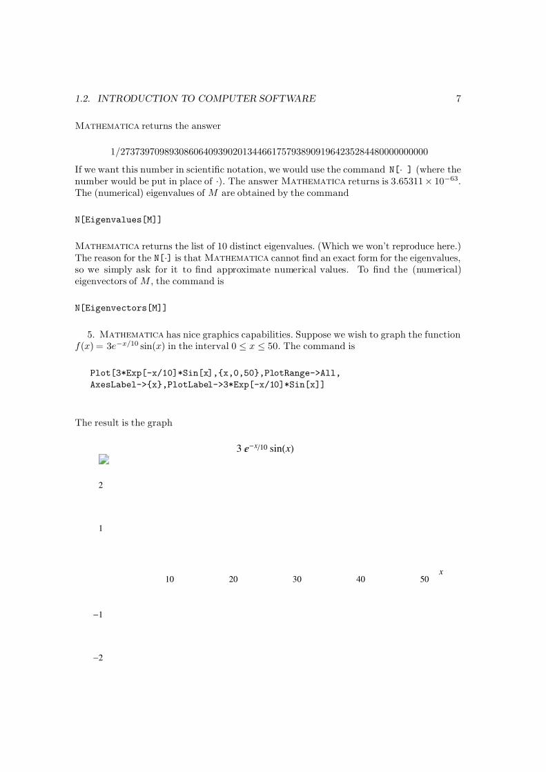
5. Mathematica has nice graphics capabilities. Suppose we wish to graph the functionf (x) = 3e−x/10 sin(x) in the interval 0 ≤ x ≤ 50. The command is

Plot[3*Exp[-x/10]*Sin[x],x,0,50,PlotRange->All,

AxesLabel->x,PlotLabel->3*Exp[-x/10]*Sin[x]]

The result is the graph

10 20 30 40 50 x

2

1

1

2

3 x 10 sin x

7/27/2019 22BBook.pdf



1.3 Exercises

#1. MatLab and/or Mathematica Exercises

1. Use MatLab or Mathematica to get an estimate (in scientific notation) of 9999. Nowuse

>> help format

to learn how to get more decimal places. (All MatLab computations are done to arelative precision of about 16 decimal places. MatLab defaults to printing out thefirst 5 digits.) Thus entering

>> format long e

on a command line and then re-entering the above computation will give the 16 digitanswer.

In Mathematica to get 16 digits accuracy the command is

N[99^(99),16]

Ans.: 3.697296376497268 × 10197.

2. Use MatLab to compute

sin(π/7). (Note that MatLab has the special symbol pi;that is pi ≈ π = 3.14159 . . . to 16 digits accuracy.)

In Mathematica the command is

N[Sqrt[Sin[Pi/7]],16]

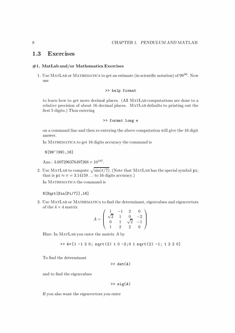
3. Use MatLab or Mathematica to find the determinant, eigenvalues and eigenvectorsof the 4 × 4 matrix

A =

1 −1 2 0√ 2 1 0 −2

0 1√

2 −11 2 2 0

Hint: In MatLab you enter the matrix A by

>> A=[1 -1 2 0; sqrt(2) 1 0 -2;0 1 sqrt(2) -1; 1 2 2 0]

To find the determinant

>> det(A)

and to find the eigenvalues

>> eig(A)

If you also want the eigenvectors you enter

7/27/2019 22BBook.pdf


1.3. EXERCISES 9

>> [V,D]=eig(A)

In this case the columns of V are the eigenvectors of A and the diagonal elements of D are the corresponding eigenvalues. Try this now to find the eigenvectors. For thedeterminant you should get the result 16.9706. One may also calculate the determi-nant symbolically. First we tell MatLab that A is to be treated as a symbol (we areassuming you have already entered A as above):

>> A=sym(A)

and then re-enter the command for the determinant

det(A)

and this time MatLab returns

ans =

12*2^(1/2)

that is, 12√

2 which is approximately equal to 16.9706.

4. Use MatLab or Mathematica to plot sin θ and compare this with the approximationsin θ ≈ θ. For 0 ≤ θ ≤ π/2, plot both on the same graph.

#2. Inverted Pendulum

This exercise derives the small angle approximation to (1.8) when the pendulum is nearly

inverted, i.e. θ ≈ π. Introduceφ = θ − π

and derive a small φ-angle approximation to (1.8). How does the result differ from (1.9)?

7/27/2019 22BBook.pdf



7/27/2019 22BBook.pdf


Chapter 2

First Order Equations

A differential equation is an equation between specified derivatives of an unknownfunction, its values, and known quantities and functions. Many physical laws aremost simply and naturally formulated as differential equations (or DEs, as wewill write for short). For this reason, DEs have been studied by the greatestmathematicians and mathematical physicists since the time of Newton.

Ordinary differential equations are DEs whose unknowns are functions of a singlevariable; they arise most commonly in the study of dynamical systems and elec-trical networks. They are much easier to treat than partial differential equations,whose unknown functions depend on two or more independent variables.

Ordinary DEs are classified according to their order. The order of a DE isdefined as the largest positive integer, n, for which the nth derivative occurs inthe equation. Thus, an equation of the form

φ(x,y,y′) = 0

is said to be of the first order .

G. Birkhoff and G-C Rota, Ordinary Differential equations , 4th ed. [3].

2.1 Linear First Order Equations

2.1.1 Introduction

The simplest differential equation is one you already know from calculus; namely,

dy

dx = f (x). (2.1)

To find a solution to this equation means one finds a function y = y(x) such that itsderivative, dy/dx, is equal to f (x). The fundamental theorem of calculus tells us that allsolutions to this equation are of the form

y(x) = y0 +

xx0

f (s) ds. (2.2)

Remarks:

11

7/27/2019 22BBook.pdf


12 CHAPTER 2. FIRST ORDER EQUATIONS

• y(x0) = y0 and y0 is arbitrary. That is, there is a one-parameter family of solutions;y = y(x; y0) to (2.1). The solution is unique once we specify the initial condition

y(x0) = y0. This is the solution to the initial value problem. That is, we have founda function that satisfies both the ODE and the initial value condition.

• Every calculus student knows that differentiation is easier than integration. Observethat solving a differential equation is like integration—you must find a function suchthat when it and its derivatives are substituted into the equation the equation isidentically satisfied. Thus we sometimes say we “integrate” a differential equation. Inthe above case it is exactly integration as you understand it from calculus. This alsosuggests that solving differential equations can be expected to be difficult.

• For the integral to exist in (2.2) we must place some restrictions on the function f appearing in (2.1); here it is enough to assume f is continuous on the interval [a, b].It was implicitly assumed in (2.1) that x was given on some interval—say [a, b].

A simple generalization of (2.1) is to replace the right-hand side by a function thatdepends upon both x and y

dy

dx= f (x, y).

Some examples are f (x, y) = xy2, f (x, y) = y, and the case (2.1). The simplest choice interms of the y dependence is for f (x, y) to depend linearly on y. Thus we are led to study

dy

dx= g(x) − p(x)y,

where g(x) and p(x) are functions of x. We leave them unspecified. (We have put the minussign into our equation to conform with the standard notation.) The conventional way towrite this equation is

dy

dx+ p(x)y = g(x). (2.3)

It’s possible to give an algorithm to solve this ODE for more or less general choices of p(x)and g(x). We say more or less since one has to put some restrictions on p and g—that theyare continuous will suffice. It should be stressed at the outset that this ability to find anexplicit algorithm to solve an ODE is the exception—most ODEs encountered will not beso easily solved.

2.1.2 Method of Integrating Factors

If (2.3) were of the form (2.1), then we could immediately write down a solution in termsof integrals. For (2.3) to be of the form (2.1) means the left-hand side is expressed as thederivative of our unknown quantity. We have some freedom in making this happen—forinstance, we can multiply (2.3) by a function, call it µ(x), and ask whether the resultingequation can be put in form (2.1). Namely, is

µ(x)dy

dx+ µ(x) p(x)y =

d

dx(µ(x)y) ? (2.4)

7/27/2019 22BBook.pdf


2.1. LINEAR FIRST ORDER EQUATIONS 13

Taking derivatives we ask can µ be chosen so that

µ(x) dydx + µ(x) p(x)y = µ(x) dydx + dµdx y

holds? This immediately simplifies to1

µ(x) p(x) =dµ

dx,

ord

dxlog µ(x) = p(x).

Integrating this last equation gives

log µ(x) =

p(s) ds + c.

Taking the exponential of both sides (one can check later that there is no loss in generalityif we set c = 0) gives2

µ(x) = exp

x p(s) ds

. (2.5)

Defining µ(x) by (2.5), the differential equation (2.4) is transformed to

d

dx(µ(x)y) = µ(x)g(x).

This last equation is precisely of the form (2.1), so we can immediately conclude

µ(x)y(x) =

xµ(s)g(s) ds + c,

and solving this for y gives our final formula

y(x) =1

µ(x)

xµ(s)g(s) ds +

c

µ(x), (2.6)

where µ(x), called the integrating factor , is defined by (2.5). The constant c will be deter-mined from the initial condition y(x0) = y0.

2.1.3 Application to Mortgage Payments

Suppose an amount P , called the principal, is borrowed at an interest I (100I%) for a periodof N years. One is to make monthly payments in the amount D/12 (D equals the amountpaid in one year). The problem is to find D in terms of P , I and N . Let

y(t) = amount owed at time t (measured in years).

1Notice y and its first derivative drop out. This is a good thing since we wouldn’t want to express µ interms of the unknown quantity y.

2By the symbolR x f (s) ds we mean the indefinite integral of f in the variable x.

7/27/2019 22BBook.pdf



We have the initial condition

y(0) = P (at time 0 the amount owed is P ).

We are given the additional information that the loan is to be paid off at the end of N years,

y(N ) = 0.

We want to derive an ODE satisfied by y. Let ∆t denote a small interval of time and ∆ythe change in the amount owed during the time interval ∆t. This change is determined by

• ∆y is increased by compounding at interest I ; that is, ∆y is increased by the amountIy(t)∆t.

• ∆y is decreased by the amount paid back in the time interval ∆t. If D denotes this

constant rate of payback, then D∆t is the amount paid back in the time interval ∆t.

Thus we have∆y = Iy∆t − D∆t,

or∆y

∆t= Iy − D.

Letting ∆t → 0 we obtain the sought after ODE,

dy

dt= Iy − D. (2.7)

This ODE is of form (2.3) with p =−

I and g =−

D. One immediately observes that thisODE is not exactly what we assumed above, i.e. D is not known to us. Let us go ahead andsolve this equation for any constant D by the method of integrating factors. So we chooseµ according to (2.5),

µ(t) := exp

t p(s) ds

= exp

− t

I ds

= exp(−It).

Applying (2.6) gives

y(t) = 1µ(t)

tµ(s)g(s) ds + c

µ(t)

= eIt

te−Is(−D) ds + ceIt

= −DeIt

−1

I e−It

+ ceIt

=D

I + ceIt .

7/27/2019 22BBook.pdf


2.1. LINEAR FIRST ORDER EQUATIONS 15

The constant c is fixed by requiringy(0) = P,

that isD

I + c = P.

Solving this for c gives c = P −D/I . Substituting this expression for c back into our solutiony(t) gives

y(t) =D

I −

D

I − P

eIt .

First observe that y(t) grows if D/I < P . (This might be a good definition of loan sharking!)We have not yet determined D. To do so we use the condition that the loan is to be paidoff at the end of N years, y(N ) = 0. Substituting t = N into our solution y(t) and usingthis condition gives

0 = DI −DI − P

eNI .

Solving for D,

D = P I eNI

eNI − 1, (2.8)

gives the sought after relation between D, P , I and N . For example, if P = $100, 000,I = 0.06 (6% interest) and the loan is for N = 30 years, then D = $7, 188.20 so themonthly payment is D/12 = $599.02. Some years ago the mortgage rate was 12%. A quickcalculation shows that the monthly payment on the same loan at this interest would havebeen $1028.09.

We remark that this model is a continuous model—the rate of payback is at the continuousrate D. In fact, normally one pays back only monthly. Banks, therefore, might want to takethis into account in their calculations. I’ve found from personal experience that the abovemodel predicts the bank’s calculations to within a few dollars.

Suppose we increase our monthly payments by, say, $50. (We assume no prepaymentpenalty.) This $50 goes then to paying off the principal. The problem then is how long doesit take to pay off the loan? It is an exercise to show that the number of years is (D is thetotal payment in one year)

− 1

I log

1 − P I

D

. (2.9)

Another questions asks on a loan of N years at interest I how long does it take to pay off one-half of the principal? That is, we are asking for the time T when

y(T ) =P

2 .

It is an exercise to show that

T =1

I log

1

2(eNI + 1)

. (2.10)

For example, a 30 year loan at 9% is half paid off in the 23rd year. Notice that T does notdepend upon the principal P .

7/27/2019 22BBook.pdf



2.2 Separation of Variables Applied to Mechanics

2.2.1 Energy Conservation

Consider the motion of a particle of mass m in one dimension, i.e. the motion is along aline. We suppose that the force acting at a point x, F (x), is conservative . This means thereexists a function V (x), called the potential energy , such that

F (x) = −dV

dx.

(Tradition has it we put in a minus sign.) In one dimension this requires that F is only afunction of x and not x (= dx/dt) which physically means there is no friction. In higher

spatial dimensions the requirement that F is conservative is more stringent. The concept of conservation of energy is that

E = Kinetic energy + Potential energy

does not change with time as the particle’s position and velocity evolves according to New-ton’s equations. We now prove this fundamental fact. We recall from elementary physicsthat the kinetic energy (KE) is given by

KE =1

2mv2, v = velocity = x.

Thus the energy is

E = E (x, x) =1

2m

dx

dt

2+ V (x).

To show that E = E (x, x) does not change with t when x = x(t) satisfies Newton’s equations,

we differentiate E with respect to t and show the result is zero:dE

dt= m

dx

dt

d2x

dt2+

dV

dx

dx

dt(by the chain rule)

=dx

dt

m

d2x

dt2+

dV (x)

dx

=dx

dt

m

d2x

dt2− F (x)

.

Now not any function x = x(t) describes the motion of the particle—x(t) must satisfy

F = md2x

dt2,

and we now get the desired resultdE

dt= 0.

This implies that E is constant on solutions to Newton’s equations.

We now use energy conservation and what we know about separation of variables to solvethe problem of the motion of a point particle in a potential V (x). Now

E =1

2m

dx

dt

2+ V (x) (2.11)

http://en.wikipedia.org/wiki/Kinetic_energy

http://en.wikipedia.org/wiki/Kinetic_energy

7/27/2019 22BBook.pdf


2.2. SEPARATION OF VARIABLES APPLIED TO MECHANICS 17

is a nonlinear first order differential equation. (We know it is nonlinear since the firstderivative is squared.) We rewrite the above equation as

dx

dt

2=

2

m(E − V (x)) ,

ordx

dt= ±

2

m(E − V (x)) .

(In what follows we take the + sign, but in specific applications one must keep in mind thepossibility that the − sign is the correct choice of the square root.) This last equation is of the form in which we can separate variables. We do this to obtain

dx

2m

(E −

V (x))= dt.

This can be integrated to

±

1 2m (E − V (x))

dx = t − t0.(2.12)

2.2.2 Hooke’s Law

Consider a particle of mass m subject to the force

F = −kx, k > 0, (Hooke’s Law). (2.13)

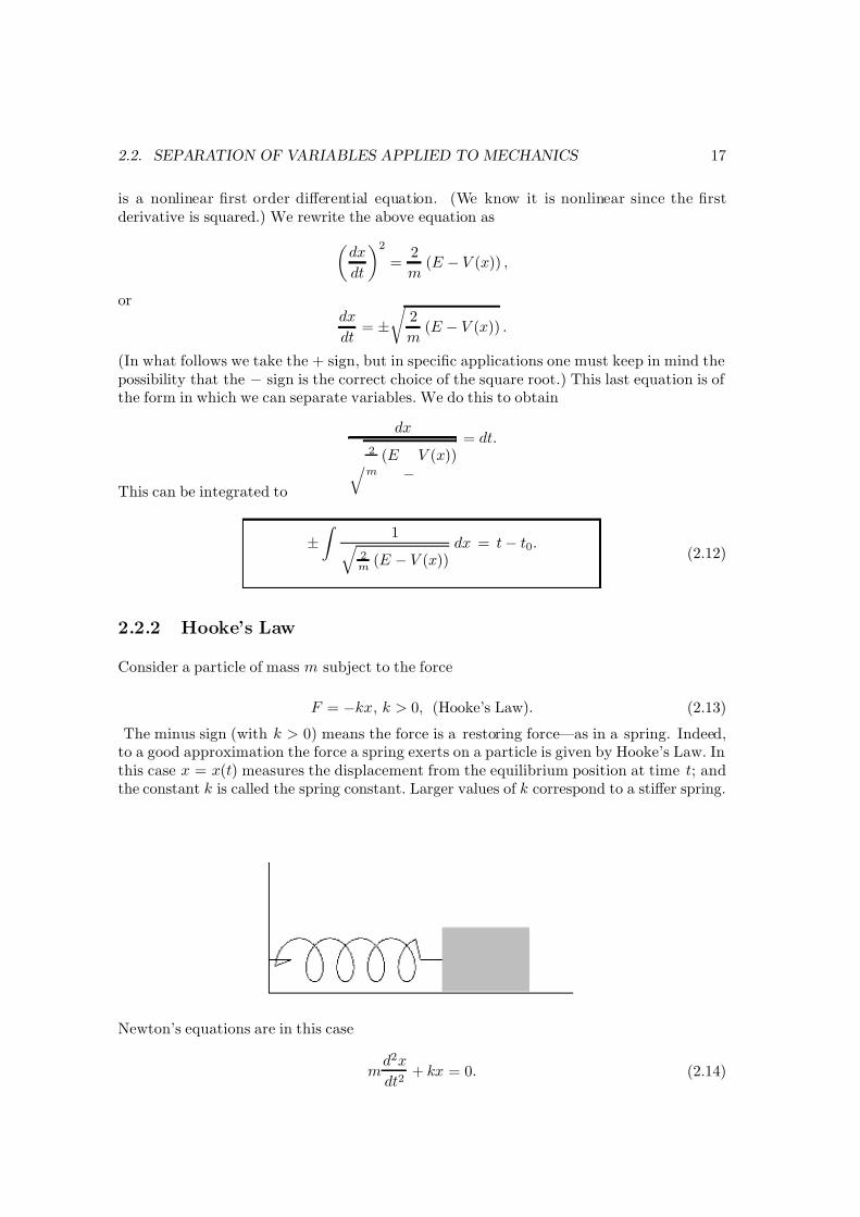
The minus sign (with k > 0) means the force is a restoring force—as in a spring. Indeed,to a good approximation the force a spring exerts on a particle is given by Hooke’s Law. Inthis case x = x(t) measures the displacement from the equilibrium position at time t; andthe constant k is called the spring constant. Larger values of k correspond to a stiffer spring.

Newton’s equations are in this case

md2x

dt2+ kx = 0. (2.14)

7/27/2019 22BBook.pdf



This is a second order linear differential equation, the subject of the next chapter. However,we can use the energy conservation principle to derive an associated nonlinear first order

equation as we discussed above. To do this, we first determine the potential correspondingto Hooke’s force law.

One easily checks that the potential equals

V (x) =1

2k x2.

(This potential is called the harmonic potential .) Let’s substitute this particular V into(2.12):

1 2E/m − kx2/m

dx = t − t0. (2.15)

Recall the indefinite integral dx√

a2 − x2= arcsin

x|a|

+ c.

Using this in (2.15) we obtain 1

2E/m − kx2/mdx =

1 k/m

dx

2E/k − x2

=1

k/marcsin

x

2E/k

+ c.

Thus (2.15) becomes3

arcsin x 2E/k

= km

t + c.

Taking the sine of both sides of this equation gives

x 2E/k

= sin

k

mt + c

,

or

x(t) =

2E

ksin

k

mt + c

. (2.16)

Observe that there are two constants appearing in (2.16), E and c. Suppose one initialcondition is

x(0) = x0.

Evaluating (2.16) at t = 0 gives

x0 =

2E

ksin(c). (2.17)

Now use the sine addition formula,

sin(θ1 + θ2) = sin θ1 cos θ2 + sin θ2 cos θ1,

3We use the same symbol c for yet another unknown constant.

7/27/2019 22BBook.pdf



in (2.16):

x(t) =

2E k

sin

km

t

cos c + cos

km

t

sin c

=

2E

ksin

k

mt

cos c + x0 cos

k

mt

(2.18)

where we use (2.17) to get the last equality.

Now substitute t = 0 into the energy conservation equation,

E =1

2mv20 + V (x0) =

1

2mv20 +

1

2k x20.

(v0

equals the velocity of the particle at time t = 0.) Substituting (2.17) in the right handside of this equation gives

E =1

2mv20 +

1

2k

2E

ksin2 c

or

E (1 − sin2 c) =1

2mv20.

Recalling the trig identity sin2 θ + cos2 θ = 1, this last equation can be written as

E cos2 c =1

2mv20.

Solve this for v0 to obtain the identity

v0 =

2E

mcos c.

We now use this in (2.18)

x(t) = v0

m

ksin

k

mt

+ x0 cos

k

mt

.

To summarize, we have eliminated the two constants E and c in favor of the constants x0and v0. As it must be, x(0) = x0 and x(0) = v0. The last equation is more easily interpretedif we define

ω0 = km

. (2.19)

Observe that ω0 has the units of 1/time, i.e. frequency. Thus our final expression for theposition x = x(t) of a particle of mass m subject to Hooke’s Law is

x(t) = x0 cos(ω0t) +v0ω0

sin(ω0t). (2.20)

7/27/2019 22BBook.pdf



Observe that this solution depends upon two arbitrary constants, x0 and v0.4 In (2.6), thegeneral solution depended only upon one constant. It is a general fact that the number of

independent constants appearing in the general solution of a nth order5 ODE is n.

Period of Mass-Spring System Satisfying Hooke’s Law

The sine and cosine are periodic functions of period 2π, i.e.

sin(θ + 2π) = sin θ, cos(θ + 2π) = cos θ.

This implies that our solution x = x(t) is periodic in time,

x(t + T ) = x(t),

where the period T is

T =2π

ω0= 2π

m

k. (2.22)

2.2.3 Period of the Nonlinear Pendulum

In this section we use the method of separation of variables to derive an exact formula for theperiod of the pendulum. Recall that the ODE describing the time evolution of the angle of deflection, θ, is (1.8). This ODE is a second order equation and so the method of separationof variables does not apply to this equation. However, we will use energy conservation in amanner similar to the previous section on Hooke’s Law.

To get some idea of what we should expect, first recall the approximation we derived forsmall deflection angles, (1.9). Comparing this differential equation with (2.14), we see thatunder the identification x → θ and k

m → gℓ , the two equations are identical. Thus using the

period derived in the last section, (2.22), we get as an approximation to the period of thependulum

T 0 =2π

ω0= 2π

ℓ

g. (2.23)

An important feature of T 0 is that it does not depend upon the amplitude of the oscillation.6

That is, suppose we have the initial conditions7

θ(0) = θ0, θ(0) = 0, (2.24)

4ω0 is a constant too, but it is a parameter appearing in the differential equation that is fixed by the

mass m and the spring constant k. Observe that we can rewrite (2.14) asx + ω2

0x = 0. (2.21)

Dimensionally this equation is pleasing: x has the dimensions of d/t2 (d is distance and t is time) and sodoes ω2

0x since ω0 is a frequency. It is instructive to substitute (2.20) into (2.21) and verify directly that it

is a solution. Please do so!5The order of a scalar differential equation is equal to the order of the highest derivative appearing in

the equation. Thus (2.3) is first order whereas (2.14) is second order.6Of course, its validity is only for small oscillations.7For simplicity we assume the initial angular velocity is zero, θ(0) = 0. This is the usual initial condition

for a pendulum.

7/27/2019 22BBook.pdf



then T 0 does not depend upon θ0. We now proceed to derive our formula for the period, T ,of the pendulum.

We claim that the energy of the pendulum is given by

E = E (θ, θ) =1

2mℓ2 θ2 + mgℓ(1 − cos θ). (2.25)

Proof of (2.25)

We begin with

E = Kinetic energy + Potential energy

=1

2mv2 + mgy. (2.26)

(This last equality uses the fact that the potential at height h in a constant gravitationalforce field is mgh. In the pendulum problem with our choice of coordinates h = y.) The xand y coordinates of the pendulum ball are, in terms of the angle of deflection θ, given by

x = ℓ sin θ, y = ℓ(1 − cos θ).

Differentiating with respect to t gives

x = ℓ cos θ θ, y = ℓ sin θ θ,

from which it follows that the velocity is given by

v2 = x2 + y2

= ℓ

2 ˙θ

2

.Substituting these in (2.26) gives (2.25).

The energy conservation theorem states that for solutions θ(t) of (1.8), E (θ(t), θ(t)) isindependent of t. Thus we can evaluate E at t = 0 using the initial conditions (2.24) andknow that for subsequent t the value of E remains unchanged,

E =1

2mℓ2 θ(0)2 + mgℓ (1 − cos θ(0))

= mgℓ(1 − cos θ0).

Using this (2.25) becomes

mgℓ(1 − cos θ0) =

1

2 mℓ

2 ˙θ

2

+ mgℓ(1 − cos θ),

which can be rewritten as

1

2mℓ2θ2 = mgℓ(cos θ − cos θ0).

Solving for θ,

θ =

2g

ℓ(cos θ − cos θ0) ,

7/27/2019 22BBook.pdf



followed by separating variables gives

dθ 2gℓ (cos θ − cos θ0)

= dt. (2.27)

We now integrate (2.27). The next step is a bit tricky—to choose the limits of integrationin such a way that the integral on the right hand side of (2.27) is related to the period T .By the definition of the period, T is the time elapsed from t = 0 when θ = θ0 to the time T when θ first returns to the point θ0. By symmetry, T /2 is the time it takes the pendulumto go from θ0 to −θ0. Thus if we integrate the left hand side of (2.27) from −θ0 to θ0 thetime elapsed is T /2. That is,

1

2T =

θ0

−θ0

dθ

2gℓ (cos θ − cos θ0)

.

Since the integrand is an even function of θ,

T = 4

θ00

dθ 2gℓ (cos θ − cos θ0)

. (2.28)

This is the sought after formula for the period of the pendulum. For small θ0 we expectthat T , as given by (2.28), should be approximately equal to T 0 (see (2.23)). It is instructive

to see this precisely.We now assume |θ0| ≪ 1 so that the approximation

cos θ ≈ 1 − 1

2!θ2 +

1

4!θ4

is accurate for |θ| < θ0. Using this approximation we see that

cos θ − cos θ0 ≈ 1

2!(θ20 − θ2) − 1

4!(θ40 − θ4)

=1

2(θ20 − θ2)

1 − 1

12(θ20 + θ2)

.

From Taylor’s formula8

we get the approximation, valid for |x| ≪ 1,1√

1 − x≈ 1 +

1

2x.

8You should be able to do this without resorting to MatLab . But if you wanted higher order termsMatLab would be helpful. Recall to do this we would enter

>> syms x

>> taylor(1/sqrt(1-x))

7/27/2019 22BBook.pdf



Thus

1 2gℓ (cos θ − cos θ0)

≈

ℓg

1 θ20 − θ2

1 1 − 1

12 (θ20 + θ2)

≈

ℓ

g

1 θ20 − θ2

1 +

1

24(θ20 + θ2)

.

Now substitute this approximate expression for the integrand appearing in (2.28) to find

T

4=

ℓ

g

θ00

1 θ20 − θ2

1 +

1

24(θ20 + θ2)

+ higher order corrections.

Make the change of variables θ = θ0x, then θ00

dθ θ20 − θ2

=

10

dx√ 1 − x2

=π

2,

θ00

θ2 dθ θ20 − θ2

= θ20

10

x2 dx√ 1 − x2

= θ20π

4.

Using these definite integrals we obtain

T

4=

ℓ

g

π

2+

1

24(θ20

π

2+ θ20

π

4)

= ℓ

g

π

2 1 +θ2016+ higher order terms.

Recalling (2.23), we conclude

T = T 0

1 +

θ2016

+ · · ·

(2.29)

where the · · · represent the higher order correction terms coming from higher order termsin the expansion of the cosines. These higher order terms will involve higher powers of θ0.It now follows from this last expression that

limθ0→0

T = T 0.

Observe that the first correction term to the linear result, T 0, depends upon the initialamplitude of oscillation θ0.

Remark: To use MatLab to evaluate symbolically these definite integrals you enter (notethe use of ’)

>> int(’1/sqrt(1-x^2)’,0,1)

and similarly for the second integral

>> int(’x^2/sqrt(1-x^2)’,0,1)

7/27/2019 22BBook.pdf



Numerical Example

Suppose we have a pendulum of length ℓ = 1 meter. The linear theory says that the periodof the oscillation for such a pendulum is

T 0 = 2π

ℓ

g= 2π

1

9.8= 2.0071 sec.

If the amplitude of oscillation of the of the pendulum is θ0 ≈ 0.2 (this corresponds to roughlya 20 cm deflection for the one meter pendulum), then (2.29) gives

T = T 0

1 +

1

16(.2)2

= 2.0121076 sec.

One might think that these are so close that the correction is not needed. This might well

be true if we were interested in only a few oscillations. What would be the difference in oneweek (1 week=604,800 sec)?

One might well ask how good an approximation is (2.29) to the exact result (2.28)? Toanswer this we have to evaluate numerically the integral appearing in (2.28). Evaluating(2.28) numerically (using say Mathematica’s NIntegrate) is a bit tricky because the end-point θ0 is singular—an integrable singularity but it causes numerical integration routinessome difficulty. Here’s how you get around this problem. One isolates where the problemoccurs—near θ0—and takes care of this analytically. For ε > 0 and ε ≪ 1 we decomposethe integral into two integrals: one over the interval (0, θ0 − ε) and the other one over theinterval (θ0 − ε, θ0). It’s the integral over this second interval that we estimate analytically.Expanding the cosine function about the point θ0, Taylor’s formula gives

cos θ = cos θ0 − sin θ0 (θ − θ0) − cos θ02 (θ − θ0)2 + · · · .

Thus

cos θ − cos θ0 = sin θ0 (θ − θ0)

1 − 1

2cot θ0 (θ − θ0)

+ · · · .

So

1√ cos θ − cos θ0

=1

sin θ0 (θ − θ0)

1 1 − 1

2 cot θ0(θ0 − θ)+ · · ·

=1

sin θ0 (θ0 − θ)

1 +

1

4cot θ0 (θ0 − θ)

+ · · ·

Thus θ0θ0−ε

dθ√ cos θ − cos θ0

=

θ0θ0−ε

dθ sin θ0 (θ0 − θ)

1 +

1

4cot θ0 (θ − θ0)

dθ + · · ·

=1√

sin θ0

ε0

u−1/2 du +1

4cot θ0

ε0

u1/2 du + · · ·

(u := θ0 − θ)

=1√

sin θ0

2ε1/2 +

1

6cot θ0 ε3/2

+ · · · .

7/27/2019 22BBook.pdf


2.3. EXERCISES 25

Choosing ε = 10−2, the error we make in using the above expression is of order ε5/2 = 10−5.Substituting θ0 = 0.2 and ε = 10−2 into the above expression, we get the approximation θ0

θ0−ε


≈ 0.4506

where we estimate the error lies in fifth decimal place. Now the numerical integration routinein MatLab quickly evaluates this integral: θ0−ε

0


≈ 1.7764

for θ0 = 0.2 and ε = 10−2. Specifically, one enters

>> quad(’1./sqrt(cos(x)-cos(0.2))’,0,0.2-1/100)

Hence for θ0 = 0.2 we have θ0

0


≈ 0.4506 + 1.77664 = 2.2270

This impliesT ≈ 2.0121.

Thus the first order approximation (2.29) is accurate to some four decimal places whenθ0 ≤ 0.2. (The reason for such good accuracy is that the correction term to (2.29) is of orderθ40 .)

Remark: If you use MatLab to do the integral from 0 to θ0 directly, i.e.

>> quad(’1./sqrt(cos(x)-cos(0.2))’,0,0.2)

what happens? This is an excellent example of what may go wrong if one uses software

packages without thinking first ! Use help quad to find out more about numerical integrationin MatLab .

2.3 Exercises for Chapter 2

#1. Radioactive decay

Carbon 14 is an unstable (radioactive) isotope of stable Carbon 12. If Q(t) represents theamount of C14 at time t, then Q is known to satisfy the ODE

dQ

dt= −λQ

where λ is a constant. If T 1/2 denotes the half-life of C14 show that

T 1/2 =log2

λ.

Recall that the half-life T 1/2 is the time T 1/2 such that Q(T 1/2) = Q(0)/2. It is known forC14 that T 1/2 ≈ 5730 years. In Carbon 14 dating it becomes difficult to measure the levelsof C14 in a substance when it is of order 0.1% of that found in currently living material.How many years must have passed for a sample of C14 to have decayed to 0.1% of its originalvalue? The technique of Carbon 14 dating is not so useful after this number of years.

http://education.jlab.org/itselemental/ele006.html

http://education.jlab.org/itselemental/ele006.html

7/27/2019 22BBook.pdf



#2: Mortgage Payment Problem

In the problem dealing with mortgage rates, prove (2.9) and (2.10). Using MatLab orMathematica to create a table of monthly payments on a loan of $200,000 for 30 years forinterest rates from 1% to 15% in increments of 1%.

#3: Discontinuous forcing term

Solve

y′ + 2y = g(t), y(0) = 0,

where

g(t) = 1, 0 ≤ t ≤ 10, t > 1

We make the additional assumption that the solution y = y(t) should be a continuousfunction of t. Hint: First solve the differential equation on the interval [0, 1] and then onthe interval [1, ∞). You are given the initial value at t = 0 and after you solve the equationon [0, 1] you will then know y(1). This is problem #32, pg. 74 (7th edition) of the Boyce &DiPrima [4]. Write a MatLab or Mathematica program to plot the solution y = y(t) for0 ≤ t ≤ 4.

#4. Application to Population Dynamics

In biological applications the population P of certain organisms at time t is sometimesassumed to obey the equation

dP dt

= aP

1 − P E

(2.30)

where a and E are positive constants.

1. Find the equilibrium solutions. (That is solutions that don’t change with t.)

2. From (2.30) determine the regions of P where P is increasing (decreasing) as a functionof t. Again using (2.30) find an expression for d2P/dt2 in terms of P and the constantsa and E . From this expression find the regions of P where P is convex (d2P/dt2 > 0)and the regions where P is concave (d2P/dt2 < 0).

3. Using the method of separation of variables solve (2.30) for P = P (t) assuming that

at t = 0, P = P 0 > 0. Find limt→∞

P (t)

Hint: To do the integration first use the identity

1

P (1 − P/E )=

1

P +

1

E − P

4. Sketch P as a function of t for 0 < P 0 < E and for E < P 0 < ∞.

7/27/2019 22BBook.pdf


2.3. EXERCISES 27

#5: Mass-Spring System with Friction

We reconsider the mass-spring system but now assume there is a frictional force present andthis frictional force is proportional to the velocity of the particle. Thus the force acting onthe particle comes from two terms: one due to the force exerted by the spring and the otherdue to the frictional force. Thus Newton’s equations become

−kx − β x = mx (2.31)

where as before x = x(t) is the displacement from the equilibrium position at time t. β andk are positive constants. Introduce the energy function

E = E (x, x) =1

2mx2 +

1

2kx2, (2.32)

and show that if x = x(t) satisfies (2.31), then

dE dt

< 0.

What is the physical meaning of this last inequality?

#6: Nonlinear Mass-Spring System

Consider a mass-spring system where x = x(t) denotes the displacement of the mass mfrom its equilibrium position at time t. The linear spring (Hooke’s Law) assumes the forceexerted by the spring on the mass is given by ( 2.13). Suppose instead that the force F isgiven by

F = F (x) = −kx − ε x3 (2.33)

where ε is a small positive number.9 The second term represents a nonlinear correctionto Hooke’s Law. Why is it reasonable to assume that the first correction term to Hooke’sLaw is of order x3 and not x2? (Hint: Why is it reasonable to assume F (x) is an odd

function of x?) Using the solution for the period of the pendulum as a guide, find an exact

integral expression for the period T of this nonlinear mass-spring system assuming the initialconditions

x(0) = x0,dx

dt(0) = 0.

Define

z =εx2

0

2k.

Show that z is dimensionless and that your expression for the period T can be written as

T = 4ω0

10

1√ 1 − u2 + z − zu4 du (2.34)

where ω0 =

k/m. We now assume that z ≪ 1. (This is the precise meaning of theparameter ε being small.) Taylor expand the function

1√ 1 − u2 + z − zu4

9One could also consider ε < 0. The case ε > 0 is a called a hard spring and ε < 0 a soft spring.

7/27/2019 22BBook.pdf



in the variable z to first order. You should find

1√ 1 − u2 + z − zu4

= 1√ 1 − u2

− 1 + u2

2√

1 − u2z + O(z2).

Now use this approximate expression in the integrand of (2.34), evaluate the definite integralsthat arise, and show that the period T has the Taylor expansion

T =2π

ω0

1 − 3

4z + O(z2)

.

#7: Motion in a Central Field

A (three-dimensional) force F is called a central force 10 if the direction of F lies along the

the direction of the position vector r. This problem asks you to show that the motion of aparticle in a central force, satisfying

F = md2r

dt2, (2.35)

lies in a plane.

1. Show that M := r × p with p := mv (2.36)

is constant in t for r = r(t) satisfying (2.35). (Here v is the velocity vector and p isthe momentum vector .) The

×in (2.36) is the vector cross product. Recall (and you

may assume this result) from vector calculus that

d

dt(a × b) =

da

dt× b + a × d b

dt.

The vector M is called the angular momentum vector.

2. From the fact that M is a constant vector, show that the vector r(t) lies in a plane

perpendicular to M . Hint: Look at r · M . Also you may find helpful the vector identity

a · ( b × c) = b · (c × a) = c · (a × b).

#8: Motion in a Central Field (cont)

From the preceding problem we learned that the position vector r(t) for a particle movingin a central force lies in a plane. In this plane, let ( r, θ) be the polar coordinates of the pointr, i.e.

x(t) = r(t)cos θ(t), y(t) = r(t)sin θ(t) (2.37)

10For an in depth treatment of motion in a central field, see [1], Chapter 2, §8.

7/27/2019 22BBook.pdf


2.3. EXERCISES 29

1. In components, Newton’s equations can be written (why?)

F x = f (r)x

r = mx, F y = f (r)y

r = my (2.38)

where f (r) is the magnitude of the force F . By twice differentiating (2.37) withrespect to t, derive formulas for x and y in terms of r, θ and their derivatives. Usethese formulas in (2.38) to show that Newton’s equations in polar coordinates (andfor a central force) become

1

mf (r)cos θ = r cos θ − 2rθ sin θ − rθ2 cos θ − rθ sin θ, (2.39)

1

mf (r)sin θ = r sin θ + 2rθ cos θ − rθ2 sin θ + rθ cos θ. (2.40)

Multiply (2.39) by cos θ, (2.40) by sin θ, and add the resulting two equations to showthat

r − rθ2 = 1m f (r). (2.41)

Now multiply (2.39) by sin θ, (2.40) by cos θ, and substract the resulting two equationsto show that

2rθ + rθ = 0. (2.42)

Observe that the left hand side of (2.42) is equal to

1

r

d

dt(r2θ).

Using this observation we then conclude (why?)

r2θ = H (2.43)

for some constant H . Use (2.43) to solve for θ, eliminate θ in (2.41) to conclude that

the polar coordinate function r = r(t) satisfies

r =1

mf (r) +

H 2

r3. (2.44)

2. Equation (2.44) is of the form that a second derivative of the unknown r is equal tosome function of r. We can thus apply our general energy method to this equation.Let Φ be a function of r satisfying

1

mf (r) = −dΦ

dr,

and find an effective potential V = V (r) such that (2.44) can be written as

r =−

dV

dr(2.45)

(Ans: V (r) = Φ(r) + H 2

2r2 ). Remark: The most famous choice for f (r) is the inversesquare law

f (r) = −mMG0

r2

which describes the gravitational attraction of two particles of masses m and M . (G0

is the universal gravitational constant.) In your physics courses, this case will beanalyzed in great detail. The starting point is what we have done here.

7/27/2019 22BBook.pdf



3. With the choice

f (r) =−

mMG0

r2the equation (2.44) gives a DE that is satisfied by r as a function of t:

r = − G

r2+

H 2

r3(2.46)

where G = M G0. We now use (2.46) to obtain a DE that is satisfied by r as a functionof θ. This is the quantity of interest if one wants the orbit of the planet. Assume thatH = 0, r = 0, and set r = r(θ). First, show that by chain rule

r = r′′θ2 + r′θ. (2.47)

(Here, ′ implies the differentiation with respect to θ, and as usual, the dot refers todifferentiation with respect to time.) Then use (2.43) and (2.47) to obtain

r = r′′H 2

r4− (r′)2

2H 2

r5(2.48)

Now, obtain a second order DE of r as a function of θ from (2.46) and (2.48). Finally,by letting u(θ) = 1/r(θ), obtain a simple linear constant coefficient DE

u′′ + u =G

H 2(2.49)

which is known as Binet’s equation .11

#9: Euler’s Equations for a Rigid Body with No Torque

In mechanics one studies the motion of a rigid body12 around a stationary point in theabsence of outside forces. Euler’s equations are differential equations for the angular velocityvector Ω = (Ω1, Ω2, Ω3). If I i denotes the moment of inertia of the body with respect to theith principal axis, then Euler’s equations are

I 1dΩ1

dt= (I 2 − I 3)Ω2Ω3

I 2dΩ2

dt= (I 3 − I 1)Ω3Ω1

I 3dΩ3

dt= (I 1 − I 2)Ω1Ω2

Prove that

M = I 21Ω21 + I 22Ω22 + I 23Ω23

and

E =1

2I 1Ω2

1 +1

2I 2Ω2

2 +1

2I 3Ω2

3

are both first integrals of the motion. (That is, if the Ω j evolve according to Euler’s equa-tions, then M and E are independent of t.)

11For further discussion of Binet’s equation see [6].12For an in-depth discussion of rigid body motion see Chapter 6 of [1].

7/27/2019 22BBook.pdf


2.3. EXERCISES 31

#10. Exponential function

In calculus one defines the exponential function et by

et := limn→∞

(1 +t

n)n , t ∈ R.

Suppose one took the point of view of differential equations and defined et to be the (unique)solution to the ODE

dE

dt= E

that satisfies the initial condition E (0) = 1.13 Prove that the addition formula

et+s = etes

follows from the ODE definition. [Hint: Define

φ(t) := E (t + s) − E (t)E (s)

where E (t) is the above unique solution to the ODE satisfying E (0) = 1. Show that φsatisfies the ODE

dφ

dt= φ(t)

From this conclude that necessarily φ(t) = 0 for all t.]

Using the above ODE definition of E (t) show that

t0

E (s) ds = E (t) − 1.

Let E 0(t) = 1 and define E n(t), n ≥ 1 by

E n+1(t) = 1 +

t0

E n(s) ds, n = 0, 1, 2, . . . . (2.50)

Show that

E n(t) = 1 + t +t2

2!+ · · · +

tn

n!.

By the ratio test this sequence of partial sums converges as n → ∞. Assuming one can takethe limit n → ∞ inside the integral (2.50), conclude that

e

t

= E (t) =

∞n=0

tn

n!

13That is, we are taking the point of view that we define et to be the solution E (t).

7/27/2019 22BBook.pdf



7/27/2019 22BBook.pdf


Chapter 3

Second Order Linear Equations

Figure 3.1: eix = cos +i sin x, Leonhard Euler, Introductio in Analysin Infinitorum , 1748

33

7/27/2019 22BBook.pdf


34 CHAPTER 3. SECOND ORDER LINEAR EQUATIONS

3.1 Theory of Second Order Equations

3.1.1 Vector Space of Solutions

First order linear differential equations are of the form

dy

dx+ p(x)y = f (x). (3.1)

Second order linear differential equations are linear differential equations whose highestderivative is second order:

d2y

dx2+ p(x)

dy

dx+ q (x)y = f (x). (3.2)

If f (x) = 0,d2y

dx2+ p(x)

dy

dx+ q (x)y = 0, (3.3)

the equation is called homogeneous . For the discussion here, we assume p and q are contin-uous functions on a closed interval [a, b]. There are many important examples where thiscondition fails and the points at which either p or q fail to be continuous are called singular

points . An introduction to singular points in ordinary differential equations can be foundin Boyce $ DiPrima [4]. Here are some important examples where the continuity conditionfails.

Legendre’s equation

p(x) =

−2x

1 − x2, q (x) =

n(n + 1)

1 − x2

.

At the points x = ±1 both p and q fail to be continuous.

Bessel’s equation

p(x) =1

x, q (x) = 1 − ν 2

x2.

At the point x = 0 both p and q fail to be continuous.

We saw that a solution to (3.1) was uniquely specified once we gave one initial condition,

y(x0) = y0.

In the case of second order equations we must give two initial conditions to specify uniquelya solution:

y(x0) = y0 and y′(x0) = y1. (3.4)

This is a basic theorem of the subject. It says that if p and q are continuous on someinterval (a, b) and a < x0 < b, then there exists an unique solution to (3.3) satisfying theinitial conditions (3.4).1 We will not prove this theorem in this class. As an example of the

1See Theorem 3.2.1 in the [4], pg. 131 or chapter 6 of [3]. These theorems dealing with the existence anduniqueness of the initial value problem are covered in an advanced course in differential equations.

7/27/2019 22BBook.pdf


3.1. THEORY OF SECOND ORDER EQUATIONS 35

appearance to two constants in the general solution, recall that the solution of the harmonicoscillator

x + ω20x = 0

contained x0 and v0.

Let V denote the set of all solutions to (3.3). The most important feature of V is thatit is a two-dimensional vector space . That it is a vector space follows from the linearity of (3.3). (If y1 and y2 are solutions to (3.3), then so is c1y1 + c2y2 for all constants c1 and c2.)To prove that the dimension of V is two, we first introduce two special solutions. Let Y 1and Y 2 be the unique solutions to (3.3) that satisfy the initial conditions

Y 1(0) = 1, Y ′1(0) = 0, and Y 2(0) = 0, Y ′2(0) = 1,

respectively.

We claim that

Y 1, Y 2

forms a basis for

V . To see this let y(x) be any solution to (3.3).2

Let c1 := y(0), c2 := y′(0) and

∆(x) := y(x) − c1 Y 1(x) − c2 Y 2(x).

Since y, Y 1 and Y 2 are solutions to (3.3), so too is ∆. (V is a vector space.) Observe

∆(0) = 0 and ∆′(0) = 0. (3.5)

Now the function y0(x) :≡ 0 satisfies (3.3) and the initial conditions (3.5). Since solutionsare unique, it follows that ∆(x) ≡ y0 ≡ 0. That is,

y = c1 Y 1 + c2 Y 2.

To summarize, we’ve shown every solution to (3.3) is a linear combination of Y 1 and Y 2.That Y 1 and Y 2 are linearly independent follows from their initial values: Suppose

c1Y 1(x) + c2Y 2(x) = 0.

Evaluate this at x = 0, use the initial conditions to see that c1 = 0. Take the derivative of this equation, evaluate the resulting equation at x = 0 to see that c2 = 0. Thus, Y 1 and Y 2are linearly independent. We conclude, therefore, that Y 1, Y 2 is a basis and dimV = 2.

3.1.2 Wronskians

Given two solutions y1 and y2 of (3.3) it is useful to find a simple condition that testswhether they form a basis of V . Let ϕ be the solution of (3.3) satisfying ϕ(x0) = ϕ0 andϕ′(x0) = ϕ1. We ask are there constants c1 and c2 such that

ϕ(x) = c1y1(x) + c2y2(x)

for all x? A necessary and sufficient condition that such constants exist at x = x0 is thatthe equations

ϕ0 = c1 y1(x0) + c2 y2(x0),

ϕ1 = c1 y′(x0) + c2 y′2(x0),

2We assume for convenience that x = 0 lies in the interval (a, b).

7/27/2019 22BBook.pdf



have a unique solution c1, c2. From linear algebra we know this holds if and only if thedeterminant y1(x0) y2(x0)

y′1(x0) y′2(x0)

= 0.

We define the Wronskian of two solutions y1 and y2 of (3.3) to be

W (y1, y2; x) :=

y1(x) y2(x)y′1(x) y′2(x).

= y1(x)y′2(x) − y′1(x)y2(x). (3.6)

From what we have said so far one would have to check that W (y1, y2; x) = 0 for all x toconclude y1, y2 forms a basis.

We now derive a formula for the Wronskian that will make the check necessary at onlyone point. Since y1 and y2 are solutions of (3.3), we have

y′′

1

+ p(x)y′

1

+ q (x)y1 = 0, (3.7)

y′′2 + p(x)y′2 + q (x)y2 = 0. (3.8)

Now multiply (3.7) by y2 and multiply (3.8) by y1. Subtract the resulting two equations toobtain

y1y′′2 − y′′1 y2 + p(x) (y1y′2 − y′1y2) = 0. (3.9)

Recall the definition (3.6) and observe that

dW

dx= y1y′′2 − y′′1y2.

Hence (3.9) is the equationdW

dx+ p(x)W (x) = 0, (3.10)

whose solution is

W (y1, y2; x) = c exp

− x

p(s) dx

. (3.11)

Since the exponential is never zero we see from (3.11) that either W (y1, y2; x) ≡ 0 orW (y1, y2; x) is never zero.

To summarize, to determine if y1, y2 forms a basis for V , one needs to check at only

one point whether the Wronskian is zero or not.

Applications of Wronskians

1. Claim: Suppose

y1, y2

form a basis of

V , then they cannot have a common point of

inflection in a < x < b unless p(x) and q (x) simultaneously vanish there. To provethis, suppose x0 is a common point of inflection of y1 and y2. That is,

y′′1 (x0) = 0 and y′′2 (x0) = 0.

Evaluating the differential equation (3.3) satisfied by both y1 and y2 at x = x0 gives

p(x0)y′1(x0) + q (x0)y1(x0) = 0,

p(x0)y′2(x0) + q (x0)y2(x0) = 0.

7/27/2019 22BBook.pdf


3.2. REDUCTION OF ORDER 37

Assuming that p(x0) and q (x0) are not both zero at x0, the above equations are a setof homogeneous equations for p(x0) and q (x0). The only way these equations can have

a nontrivial solution is for the determinant y′1(x0) y1(x0)y′2(x0) y2(x0)

= 0.

That is, W (y1, y2; x0) = 0. But this contradicts that y1, y2 forms a basis. Thusthere can exist no such common inflection point.

2. Claim: Suppose y1, y2 form a basis of V and that y1 has consecutive zeros at x = x1and x = x2. Then y2 has one and only one zero between x1 and x2. To prove this wefirst evaluate the Wronskian at x = x1,

W (y1, y2; x1) = y1(x1)y′2(x1) − y′1(x1)y2(x1) = −y′1(x1)y2(x1)

since y1(x1) = 0. Evaluating the Wronskian at x = x2 gives

W (y1, y2; x2) = −y′1(x2)y2(x2).

Now W (y1, y2; x1) is either positive or negative. (It can’t be zero.) Let’s assume itis positive. (The case when the Wronskian is negative is handled similarly. We leavethis case to the reader.) Since the Wronskian is always of the same sign, W (y1, y2; x2)is also positive. Since x1 and x2 are consecutive zeros, the signs of y′1(x1) and y′1(x2)are opposite of each other. But this implies (from knowing that the two Wronskianexpressions are both positive), that y2(x1) and y2(x2) have opposite signs. Thus thereexists at least one zero of y2 at x = x3, x1 < x3 < x2. If there exist two or more suchzeros, then between any two of these zeros apply the above argument (with the rolesof y1 and y2 reversed) to conclude that y1 has a zero between x1 and x2. But x1 andx2 were assumed to be consecutive zeros. Thus y2 has one and only one zero betweenx1 and x2.

In the case of the harmonic oscillator, y1(x) = cos ω0x and y2(x) = sin ω0x, and thefact that the zeros of the sine function interlace those of the cosine function is wellknown.

3.2 Reduction of Order

Suppose y1 is a solution of (3.3). Let

y(x) = v(x)y1(x).Then

y′ = v′y1 + vy′1 and y′′ = v′′y1 + 2v′y′1 + vy′′1 .

Substitute these expressions for y and its first and second derivatives into (3.3) and makeuse of the fact that y1 is a solution of (3.3). One obtains the following differential equationfor v:

v′′ +

p + 2

y′1y1

v′ = 0,

7/27/2019 22BBook.pdf



or upon setting u = v′,

u

′

+

p + 2

y′1

y1

u = 0.This last equation is a first order linear equation. Its solution is

u(x) = c exp

−

p + 2y′1y1

dx

=

c

y21(x)exp

−

p(x) dx

.

This implies

v(x) =

u(x) dx,

so that

y(x) = cy1(x)

u(x) dx.

The point is, we have shown that if one solution to (3.3) is known, then a second solution

can be found—expressed as an integral.

3.3 Constant Coefficients

We assume that p(x) and q (x) are constants independent of x. We write (3.3) in this caseas3

ay′′ + by′ + cy = 0. (3.12)

We “guess” a solution of the formy(x) = eλx.

Substituting this into (3.12) gives

aλ2eλx + bλeλx + ceλx = 0.

Since eλx is never zero, the only way the above equation can be satisfied is if

aλ2 + bλ + c = 0. (3.13)

Let λ± denote the roots of this quadratic equation, i.e.

λ± =−b ± √

b2 − 4ac

2a.

We consider three cases.

1. Assume b2 − 4ac > 0 so that the roots λ± are both real numbers. Then exp(λ+ x) andexp(λ− x) are two linearly independent solutions to (3.13). That they are solutionsfollows from their construction. They are linearly independent since

W (eλ+ x, eλ−

x; x) = (λ− − λ+)eλ+ xeλ−

x = 0

Thus in this case, every solution of (3.12) is of the form

c1 exp(λ+ x) + c2 exp(λ− x)

for some constants c1 and c2.

3This corresponds to p(x) = b/a and q(x) = c/a. For applications it is convenient to introduce theconstant a.

7/27/2019 22BBook.pdf


3.3. CONSTANT COEFFICIENTS 39

2. Assume b2 − 4ac = 0. In this case λ+ = λ−. Let λ denote their common value. Thuswe have one solution y1(x) = eλx. We could use the method of reduction of order

to show that a second linearly independent solution is y2(x) = xeλx. However, wechoose to present a more intuitive way of seeing this is a second linearly independentsolution. (One can always make it rigorous at the end by verifying that that it isindeed a solution.) Suppose we are in the distinct root case but that the two roots arevery close in value: λ+ = λ + ε and λ− = λ. Choosing c1 = −c2 = 1/ε, we know that

c1y1 + c2y2 =1

εe(λ+ε)x − 1

εeλx

= eλx eεx − 1

ε

is also a solution. Letting ε → 0 one easily checks that

eεx

−1

ε → x,

so that the above solution tends toxeλx,

our second solution. That eλx, xeλx is a basis is a simple Wronskian calculation.

3. We assume b2 − 4ac < 0. In this case the roots λ± are complex. At this point wereview the the exponential of a complex number.

Complex Exponentials

Let z = x + iy (x, y real numbers, i2 = −1) be a complex number. Recall that x iscalled the real part of z,

ℜz, and y is called the imaginary part of z,

ℑz. Just as we

picture real numbers as points lying in a line, called the real line R; we picture complexnumbers as points lying in the plane, called the complex plane C. The coordinatesof z in the complex plane are (x, y). The absolute value of z, denoted |z|, is equal to

x2 + y2. The complex conjugate of z, denoted z, is equal to x − iy. Note the usefulrelation

z z = |z|2 .

In calculus, or certainly an advanced calculus class, one considers (simple) functionsof a complex variable. For example the function

f (z) = z2

takes a complex number, z, and returns it square, again a complex number. (Can you

show that ℜf = x2

− y2

and ℑf = 2xy?). Using complex addition and multiplication,one can define polynomials of a complex variable

anzn + an−1zn−1 + · · · + a1z + a0.

The next (big) step is to study power series

∞n=0

anzn.

7/27/2019 22BBook.pdf



With power series come issues of convergence. We defer these to your advanced calculusclass.

With this as a background we are (almost) ready to define the exponential of a complexnumber z. First, we recall that the exponential of a real number x has the power seriesexpansion

ex = exp(x) =∞

n=0

xn

n!(0! := 1).

In calculus classes, one normally defines the exponential in a different way4 and thenproves ex has this Taylor expansion. However, one could define the exponential func-tion by the above formula and then prove the various properties of ex follow from thisdefinition. This is the approach we take for defining the exponential of a complexnumber except now we use a power series in a complex variable:5

ez = exp(z) :=∞

n=0

zn

n!, z ∈ C (3.14)

We now derive some properties of exp(z) based upon this definition.

• Let θ ∈ R, then

exp(iθ) =∞

n=0

(iθ)n

n!

=∞n=0

(iθ)2n

(2n)!+

∞n=0

(iθ)2n+1

(2n + 1)!

=

∞n=0

(−1)nθ2n

(2n)!+ i

∞n=0

(−1)nθ2n+1

(2n + 1)!

= cos θ + i sin θ.

This last formula is called Euler’s Formula . Two immediate consequences of Euler’s formula (and the facts cos(−θ) = cos θ and sin(θ) = − sin θ) are

exp(−iθ) = cos θ − i sin θ

exp(iθ) = exp(−iθ)

Hence

|exp(iθ)|2 = exp(iθ) exp(−iθ) = cos2 θ + sin2 θ = 1

That is, the values of exp(iθ) lie on the unit circle. The coordinates of the pointeiθ are (cos θ, sin θ).

• We claim the addition formula for the exponential function, well-known for realvalues, also holds for complex values4A common definition is ex = limn→∞(1 + x/n)n.

5It can be proved that this infinite series converges for all complex values z.

7/27/2019 22BBook.pdf


3.3. CONSTANT COEFFICIENTS 41

exp(z + w) = exp(z) exp(w), z , w ∈ C. (3.15)

We are to show

exp(z + w) =

∞n=0

1

n!(z + w)n

=∞

n=0

1

n!

nk=0

n

k

zkwn−k (binomial theorem)

is equal to

exp(z) exp(w) =∞

k=0

1

k!zk

∞m=0

1

m!wm

=∞

k,m=0

1

k!m!zkwm

=∞

n=0

nk=0

1

k!(n − k)!zkwn−k n := k + m

=∞

n=0

1

n!

nk=0

n!

k!(n − k)!zkwn−k .

Since n

k

=

n!

k!(n − k)!,

we see the two expressions are equal as claimed.

• We can now use these two properties to understand better exp( z). Let z = x+iy,then

exp(z) = exp(x + iy) = exp(x)exp(iy) = ex (cos y + i sin y) .

Observe the right hand side consists of functions from calculus. Thus with acalculator you could find the exponential of any complex number using this for-mula.6

A form of the complex exponential we frequently use is if λ = σ + iµ and x ∈ R,

then exp(λx) = exp((σ + iµ)x)) = eσx (cos(µx) + i sin(µx)) .

Returning to (3.12) in case b2 − 4ac < 0 and assuming a, b and c are all real, we seethat the roots λ± are of the form7

λ+ = σ + iµ and λ− = σ − iµ.

6Of course, this assumes your calculator doesn’t overflow or underflow in computing ex.7σ = −b/2a and µ =

√ 4ac − b2/2a.

7/27/2019 22BBook.pdf



Thus eλ+x and eλ−

x are linear combinations of

eσx

cos(µx) and eσx

sin(µx).

That they are linear independent follows from a Wronskian calculuation. To summa-rize, we have shown that every solution of (3.12) in the case b2 − 4ac < 0 is of theform

c1eσx cos(µx) + c2eσx sin(µx)

for some constants c1 and c2.

Remarks: The MatLab function exp handles complex numbers. For example,

>> exp(i*pi)

ans =

-1.0000 + 0.0000i

The imaginary unit i is i in MatLab . You can also use sqrt(-1) in place of i. This issometimes useful when i is being used for other purposes. There are also the functions

abs, angle, conj, imag real

For example,

>> w=1+2*i

w =

1.0000 + 2.0000i

>> abs(w)

ans =

2.2361

>> conj(w)

ans =

1.0000 - 2.0000i

>> real(w)

ans =

1

>> imag(w)

7/27/2019 22BBook.pdf


3.4. FORCED OSCILLATIONS OF THE MASS-SPRING SYSTEM 43

ans =

2

>> angle(w)

ans =

1.1071

3.4 Forced Oscillations of the Mass-Spring System

The forced mass-spring system is described by the differential equation

md2x

dt2+ γ

dx

dt+ k x = F (t) (3.16)

where x = x(t) is the displacement from equilibrium at time t, m is the mass, k is theconstant in Hooke’s Law, γ > 0 is the coefficient of friction, and F (t) is the forcing term. Inthese notes we examine the solution when the forcing term is periodic with period 2π/ω. (ωis the frequency of the forcing term.) The simplest choice for a periodic function is eithersine or cosine. Here we examine the choice

F (t) = F 0 cos ωt

where F 0 is the amplitude of the forcing term. All solutions to (3.16) are of the form

x(t) = x p(t) + c1x1(t) + c2x2(t) (3.17)

where x p is a particular solution of (3.16) and x1, x2 is a basis for the solution space of the homogeneous equation.

The homogeneous solutions have been discussed earlier. We know that both x1 and x2will contain a factor

e−(γ/2m)t

times factors involving sine and cosine. Since for all a > 0, e−at → 0 as t → ∞, thehomogeneous part of (3.17) will tend to zero. That is, for all initial conditions we have forlarge t to good approximation

x(t) ≈ x p(t).

Thus we concentrate on finding a particular solution x p.

With the right-hand side of (3.16) having a cosine term, it is natural to guess that theparticular solution will also involve cos ωt. If one guesses

A cos ωt

7/27/2019 22BBook.pdf



one quickly sees that due to the presence of the frictional term, this cannot be a correctsince sine terms also appear. Thus we guess

x p(t) = A cos ωt + B sin ωt (3.18)

We calculate the first and second dervatives of (3.18) and substitute the results togetherwith (3.18) into (3.16). One obtains the equation−Aω2m + Bωγ + kA

cos ωt +

−Bω2m − Aωγ + kB

sin ωt = F 0 cos ωt

This equation must hold for all t and this can happen only if −Aω2m + Bωγ + kA

= F 0 and−Bω2m − Aωγ + kB

= 0

These last two equations are a pair of linear equations for the unknown coefficients A and B.We now solve these linear equations. First we rewrite these equations to make subsequent

steps clearer: k − ω2m

A + ωγ B = F 0,

−ωγ A +

k − ω2m

B = 0.

Using Cramer’s Rule we find (check this!)

A =k − mω2

(k − mω2)2 + γ 2ω2F 0

B =γω

(k − mω2)2 + γ 2ω2F 0

We can make these results notationally simpler if we recall that the natural frequency of a(frictionless) oscillator is

ω20 = k

m

and define

∆(ω) =

m2(ω2 − ω20)2 + γ 2ω2 (3.19)

so that

A =m(ω2

0 − ω2)

∆(ω)2F 0 and B =

γω

∆(ω)2F 0

Using these expressions for A and B we can substitute into (3.18) to find our particularsolution x p. The form (3.18) is not the best form in which to understand the properties of the solution. (It is convenient for performing the above calculations.) For example, it is notobvious from (3.18) what is the amplitude of oscillation. To answer this and other questions

we introduce polar coordinates for A and B:

A = R cos δ and B = R sin δ.

Then

x p(t) = A cos ωt + B sin ωt

= R cos δ cos ωt + R sin δ sin ωt

= R cos(ωt − δ )

7/27/2019 22BBook.pdf


3.4. FORCED OSCILLATIONS OF THE MASS-SPRING SYSTEM 45

where in the last step we used the cosine addition formula. Observe that R is the amplitudeof oscillation. The quantity δ is called the phase angle . It measures how much the oscillation

lags (if δ > 0) the forcing term. (For example, at t = 0 the amplitude of the forcing term isa maximum, but the maximum oscillation is delayed until time t = δ/ω.)

Clearly,

A2 + B2 = R2 cos2 δ + R2 sin2 δ = R2

and

tan δ =B

A

Substituting the expressions for A and B into the above equations give

R2 =m2(ω2

0 − ω2)

∆4F 20 +

γ 2ω2

∆4F 20

= ∆2

∆4 F 20

=F 20∆2

Thus

R =F 0∆

(3.20)

where we recall ∆ is defined in (3.19). Taking the ratio of A and B we see that

tan δ =γω

m(ω20 − ω2)

3.4.1 Resonance

We now examine the behavior of the amplitude of oscillation, R = R(ω), as a function of the frequency ω of the driving term.

Low frequencies: When ω → 0, ∆(ω) → mω20 = k. Thus for low frequencies the amplitude

of oscillation approaches F 0/k. This result could have been anticipated since whenω → 0, the forcing term tends to F 0, a constant. A particular solution in this case isitself a constant and a quick calculation shows this constant is eqaul to F 0/k.

High frequencies: When ω → ∞, ∆(ω) ∼ mω2 and hence the amplitude of oscillationR → 0. Intuitively, if you shake the mass-spring system too quickly, it does not have

time to respond before being subjected to a force in the opposite direction; thus, theoverall effect is no motion. Observe that greater the mass (inertia) the smaller R isfor large frequencies.

Maximum Oscillation: The amplitude R is a maximum (as a function of ω) when ∆(ω)is a minimum. ∆ is a minimum when ∆2 is a minimum. Thus to find the frequencycorresponding to maximum amplitude of oscillation we must minimize

m2

ω2 − ω20

2+ γ 2ω2.

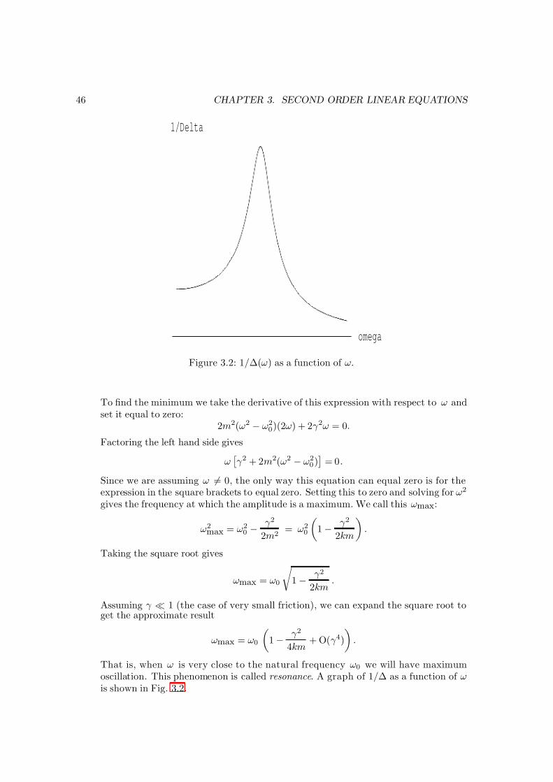
7/27/2019 22BBook.pdf



omega

1/Delta

Figure 3.2: 1/∆(ω) as a function of ω.

To find the minimum we take the derivative of this expression with respect to ω andset it equal to zero:

2m2(ω2 − ω20)(2ω) + 2γ 2ω = 0.

Factoring the left hand side gives

ω

γ 2 + 2m2(ω2 − ω20)

= 0.

Since we are assuming ω = 0, the only way this equation can equal zero is for theexpression in the square brackets to equal zero. Setting this to zero and solving for ω2

gives the frequency at which the amplitude is a maximum. We call this ωmax:

ω2max = ω2

0 − γ 2

2m2= ω2

0

1 − γ 2

2km

.

Taking the square root gives

ωmax = ω0

1 − γ 2

2km.

Assuming γ ≪ 1 (the case of very small friction), we can expand the square root toget the approximate result

ωmax = ω0

1 − γ 2

4km+ O(γ 4)

.

That is, when ω is very close to the natural frequency ω0 we will have maximumoscillation. This phenomenon is called resonance . A graph of 1/∆ as a function of ωis shown in Fig. 3.2.

7/27/2019 22BBook.pdf


3.5. EXERCISES 47

3.5 Exercises

#1. Euler’s formula

Using Euler’s formula prove the trig identity

cos(4θ) = cos4 θ − 6cos2 θ sin2 θ + sin4 θ.

Again using Euler’s formula find a formula for cos(2nθ) where n = 1, 2, . . .. In this way onecan also get identities for cos(2n + 1)θ as well as sin nθ.

#2. Roots of unity

Show that the n (distinct) solutions to the polynomial equation

xn − 1 = 0

are e2πik/n for k = 1, 2, . . . , n. For n = 6 draw a picture illustrating where these roots lie inthe complex plane.

#3. Constant coefficient ODEs

In each case find the unique solution y = y(x) that satisfies the ODE with stated initialconditions:

1. y′′ − 3y′ + 2y = 0, y(0) = 1, y′(0) = 0.

2. y′′ + 9y = 0, y(0) = 1, y′(0) = −1.

3. y′′ − 4y′ + 4y = 0, y(0) = 2, y′(0) = 0.

#4. Higher Order Equations

The third order homogeneous differential equation with constant coefficients is

a3y′′′ + a2y′′ + a1y′ + a0y = 0 (3.21)

where ai are constants. Assume a solution of the form

y(x) = eλx

and derive an equation that λ must satisfy in order that y is a solution. (You should get acubic polynomial.) What is the form of the general solution to (3.21)?

7/27/2019 22BBook.pdf



#5. Euler’s equation

A differential equation of the form

t2y′′ + aty′ + by = 0, t > 0 (3.22)

where a, b are real constants, is called Euler’s equation.8 This equation can be transformedinto an equation with constant coefficients by letting x = ln t. Solve

t2y′′ + 4ty′ + 2y = 0 (3.23)

#6 Forced undamped system

Consider a forced undamped system described by

y′′ + y = 3 cos(ωt)

with initial conditions y(0) = 1 and y′(0) = 1. Find the solution for ω = 1.

#7. Driven damped oscillator

Let

y′′ + 3y′ + 2y = 0

be the equation of a damped oscillator. If a forcing term is F (t) = 10 cos t and the oscillator

is initially at rest at the origin, what is the solution of the equation for this driven dampedoscillator? What is the phase angle?

#8. Damped oscillator

A particle is moving according to

y′′ + 10y′ + 16y = 0

with the initial condition y(0) = 1 and y′(0) = 4. Is this oscillatory ? What is the maximumvalue of y?

#9. Wronskian

Consider (3.3) with p(x) and q (x) continuous on the interval [a, b]. Prove that if two solutionsy1 and y2 have a maximum or minimum at the same point in [a, b], they cannot form a basisof V .

8There is perhaps no other mathematician whose name is associated to so many functions, identities,equations, numbers, . . . as Euler.

7/27/2019 22BBook.pdf


3.5. EXERCISES 49

#10. Euler’s equation (revisited) from physics

In Exercise 2.3.9 we obtained a set of three first-order differential equations for Ω1, Ω2 andΩ3, which are called the Euler equations when there is no torque. Let us assume thatI 1 = I 2 = I 3. (The body with these moments of inertia is called a free symmetric top.) Inthis case we have

I 1Ω1 = (I 2 − I 3)Ω2Ω3 (3.24)

I 2Ω2 = (I 3 − I 1)Ω3Ω1 (3.25)

I 3Ω3 = 0 (3.26)

Notice that Ω3 is a constant from (3.26). Show that Ω1 and Ω2 have the form of

Ω1(t) = A sin(ωt + θ0);

Ω2(t) = A cos(ωt + θ0)

where A and θ0 are some constants. Here Ω1, Ω2 and Ω3 are three components of the angularvelocity vector Ω. Show that it follows that the magnitude (length) of Ω is a constant. Findan explicit expression for ω in terms of I i and the constant Ω3.

7/27/2019 22BBook.pdf



7/27/2019 22BBook.pdf


Chapter 4

Difference Equations

Figure 4.1: Leonardo Fibonacci, c. 1170–c. 1250.

Science is what we understand well enough to explain to a computer. Art iseverything else we do.

D.E. Knuth in the preface of A=B by H. Wilf & D. Zeilberger

51

7/27/2019 22BBook.pdf


52 CHAPTER 4. DIFFERENCE EQUATIONS

4.1 Introduction

We have learned that the general inhomogeneous second order linear differential equation isof the form

a(x)d2y

dx2+ b(x)

dy

dx+ c(x)y = f (x).

The independent variable, x, takes values in R. (We say x is a continuous variable.) Manyapplications lead to problems where the independent variable is discrete ; that is, it takesvalues in the integers. Instead of y(x) we now have yn, n an integer. The discrete versionof the above equation, called an inhomogeneous second order linear difference equation , is

an yn+2 + bn yn+1 + cn yn = f n (4.1)

where we assume the sequences an, bn, cn and f n are known. For example,

(n2 + 5)yn+2 + 2yn+1 +3

n + 1yn = en, n = 0, 1, 2, 3, . . .

is such a difference equation. Usually we are given y0 and y1 (the initial values), and theproblem is to solve the difference equation for yn.

In this chapter we consider the special case of constant coefficient difference equations:

a yn+2 + b yn+1 + c yn = f n

where a, b, and c are constants independent of n. If f n = 0 we say the difference equationis homogeneous . An example of a homogeneous second order constant coefficient differenceequation is

6yn+2 +1

3 yn+1 + 2yn = 0.

4.2 Constant Coefficient Difference Equations

4.2.1 Solution of Constant Coefficient Difference Equations

In this section we give an algorithm to solve all second order homogeneous constant coeffi-cient difference equations

a yn+2 + b yn+1 + c yn = 0. (4.2)

The method is the discrete version of the method we used to solve contant coefficient differ-

ential equations. We first guess a solution of the form

yn = λn, λ = 0.

(For differential equations we guessed y(x) = eλx.) We now substitute this into (4.2) andrequire the result equal zero,

0 = aλn+2 + bλn+1 + cλn

= λn

aλ2 + bλ + c

.

7/27/2019 22BBook.pdf


4.2. CONSTANT COEFFICIENT DIFFERENCE EQUATIONS 53

This last equation is satisfied if and only if

aλ2

+ bλ + c = 0. (4.3)

Let λ1 and λ2 denote the roots of this quadratic equation. (For the moment we consideronly the case when the roots are distinct.) Then

λn1 and λn

2

are both solutions to (4.2). Just as in our study of second order ODEs, the linear combination

c1λn1 + c2λn

2

is also a solution and every solution of (4.2) is of this form. The constants c1 and c2 aredetermined once we are given the initial values y0 and y1:

y0

= c1

+ c2

,

y1 = c1λ1 + c2λ2,

are two equation that can be solved for c1 and c2.

4.2.2 Fibonnaci Numbers

Consider the sequence of numbers

1 1 2 3 5 8 13 21 34 · · ·that is, each number is the sum of the preceding two numbers starting with

1 1

as initial values. These integers are called Fibonnaci numbers and are denoted F n. Fromtheir definition, F n satisfies the difference equation

F n+1 = F n + F n−1 for n ≥ 1

withF 0 = 0, F 1 = 1.

The quadratic equation we must solve is

λ2 = λ + 1,

whose roots are

λ1,2 = 1 ± √ 52

.

SettingF n = c1λn

1 + c2λn2 ,

we see that at n = 0 and 1 we require

0 = c1 + c2,

1 = c1λ1 + c2λ2.

http://mathworld.wolfram.com/FibonacciNumber.html

http://mathworld.wolfram.com/FibonacciNumber.html

7/27/2019 22BBook.pdf



Solving these we find

c1 =

1

√ 5 , c2 = −1

√ 5 ,

and hence

F n =1√

5

1 +

√ 5

2

n

− 1√ 5

1 − √

5

2

n

.

Since λ1 > 1 and |λ2| < 1, λn1 grows with increasing n whereas λn

2 → 0 as n → ∞. Thus forlarge n

F n ∼ 1√ 5

λn1 ,

and

limn→∞

F n−1

F n

=1

λ1

:= ω.

The number

ω =

√ 5 − 1

2= 0.61803398 . . . . . .

is called the golden mean.1

4.3 Inhomogeneous Difference Equations

In a completely analogous way to the ODE case, one proves that every solution to theinhomogeneous linear difference equation (4.1) is of the form

(yn)homo + (yn)part

where (yn)homo is a solution to the homogeneous equation (4.1) with f n = 0 and (yn)part isa particular solution to the inhomogeneous equation (4.1).

4.4 Exercises

#1. Degenerate Roots

Consider the constant coefficient difference equation (4.2) but now assume the two rootsλ1,2 are equal. Show that

nλn1

is a second linearly independent solution to (4.2).

1Sometimes the number

φ = 1/ω =1 +

√ 5

2= 1.6180339887 . . .

is called the golden mean.

7/27/2019 22BBook.pdf


4.4. EXERCISES 55

#2. Rational Approximations to√

2

Solve the difference equation

xn+1 = 2xn + xn−1, n ≥ 1

with initial conditions x0 = 0 and x1 = 1 that corresponds to the sequence 0, 1, 2, 5, 12,29,.... Show that

limn→∞

xn+1 − xn

xn=

√ 2.

The rational numbersxn+1 − xn

xn

provide us with very good approximations to the square root of two.2

#3. Catalan numbers

Many times nonlinear recurrence relations arise. For example, Catalan numbers T n satisfythe nonlinear recurrence relation

T n =n−1k=0

T kT n−1−k, n = 1, 2, . . .

where T 0 := 1. Define

T (z) =∞

n=0

T nzn.

Show that

T (z) =1 − √

1 − 4z

2z.

From this prove that

T n =1

n + 1

2n

n

wherenk

is the binomial coefficient. Catalan numbers arise in a variety of combinatorial

problems. Here is one example:

Suppose 2n points are placed in fixed positions, evenly distributed on the cir-cumference of a circle. Then there are T n ways to join n pairs of the points sothat the resulting chords do not intersect.

One can easily make a table of values of T n using, say, the Mathematica command (thisgives T 1 through T 10).

Table[n, Binomial[2*n, n]/(n + 1), n, 1, 10]

2The square root of two is irrational.

http://mathworld.wolfram.com/CatalanNumber.html

http://www.math.utah.edu/~pa/math/q1.html

http://www.math.utah.edu/~pa/math/q1.html

http://mathworld.wolfram.com/CatalanNumber.html

7/27/2019 22BBook.pdf



7/27/2019 22BBook.pdf


Chapter 5

Matrix Differential Equations

Figure 5.1: Vladimir Arnold, 1937–2010.

Linear systems are almost the only large class of differential equations for whichthere exists a definitive theory. This theory is essentially a branch of linearalgebra, and allows us to solve all autonomous linear equations.

V. A. Arnold, Ordinary Differential Equations [2]

57

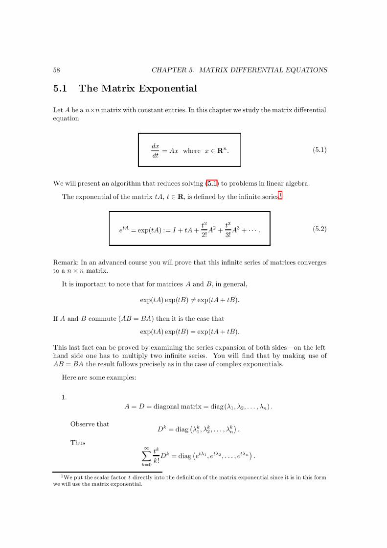
7/27/2019 22BBook.pdf


58 CHAPTER 5. MATRIX DIFFERENTIAL EQUATIONS

5.1 The Matrix Exponential

Let A be a n×n matrix with constant entries. In this chapter we study the matrix differentialequation

dx

dt= Ax where x ∈ Rn. (5.1)

We will present an algorithm that reduces solving (5.1) to problems in linear algebra.

The exponential of the matrix tA, t ∈ R, is defined by the infinite series1

etA = exp(tA) := I + tA +t2

2!A2 +

t3

3!A3 + · · · . (5.2)

Remark: In an advanced course you will prove that this infinite series of matrices convergesto a n × n matrix.

It is important to note that for matrices A and B, in general,

exp(tA) exp(tB) = exp(tA + tB).

If A and B commute (AB = BA) then it is the case that

exp(tA) exp(tB) = exp(tA + tB).

This last fact can be proved by examining the series expansion of both sides—on the lefthand side one has to multiply two infinite series. You will find that by making use of AB = BA the result follows precisely as in the case of complex exponentials.

Here are some examples:

1.

A = D = diagonal matrix = diag(λ1, λ2, . . . , λn) .

Observe thatDk = diag

λk1 , λk

2 , . . . , λkn

.

Thus∞

k=0

tk

k!Dk = diag

etλ1, etλ2 , . . . , etλn

.

1We put the scalar factor t directly into the definition of the matrix exponential since it is in this formwe will use the matrix exponential.

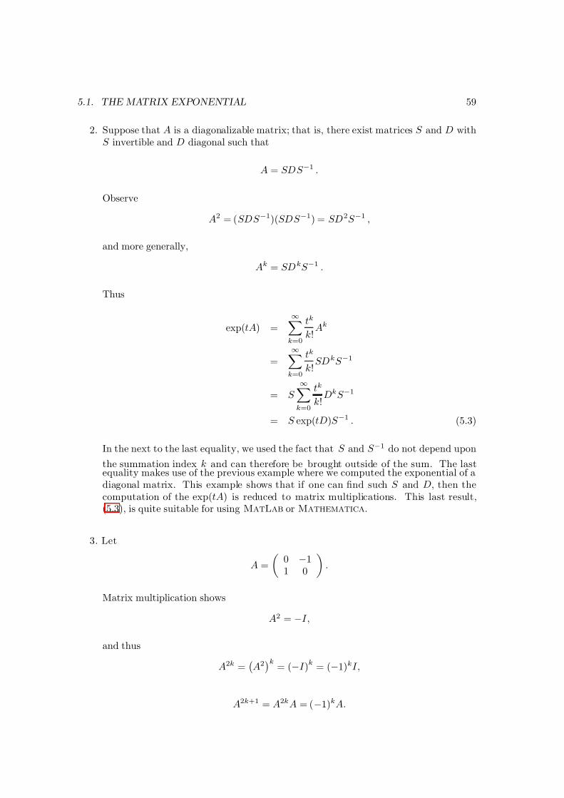
7/27/2019 22BBook.pdf


5.1. THE MATRIX EXPONENTIAL 59

2. Suppose that A is a diagonalizable matrix; that is, there exist matrices S and D withS invertible and D diagonal such that

A = SDS −1 .

Observe

A2 = (SDS −1)(SDS −1) = SD2S −1 ,

and more generally,

Ak = SDkS −1 .

Thus

exp(tA) =

∞k=0

tk

k!Ak

=

∞k=0

tk

k!SDkS −1

= S ∞

k=0

tk

k!DkS −1

= S exp(tD)S −1 . (5.3)

In the next to the last equality, we used the fact that S and S −1 do not depend upon

the summation index k and can therefore be brought outside of the sum. The lastequality makes use of the previous example where we computed the exponential of adiagonal matrix. This example shows that if one can find such S and D, then thecomputation of the exp(tA) is reduced to matrix multiplications. This last result,(5.3), is quite suitable for using MatLab or Mathematica.

3. Let

A =

0 −11 0

.

Matrix multiplication shows

A2 = −I,

and thus

A2k =

A2k

= (−I )k

= (−1)kI,

A2k+1 = A2kA = (−1)kA.

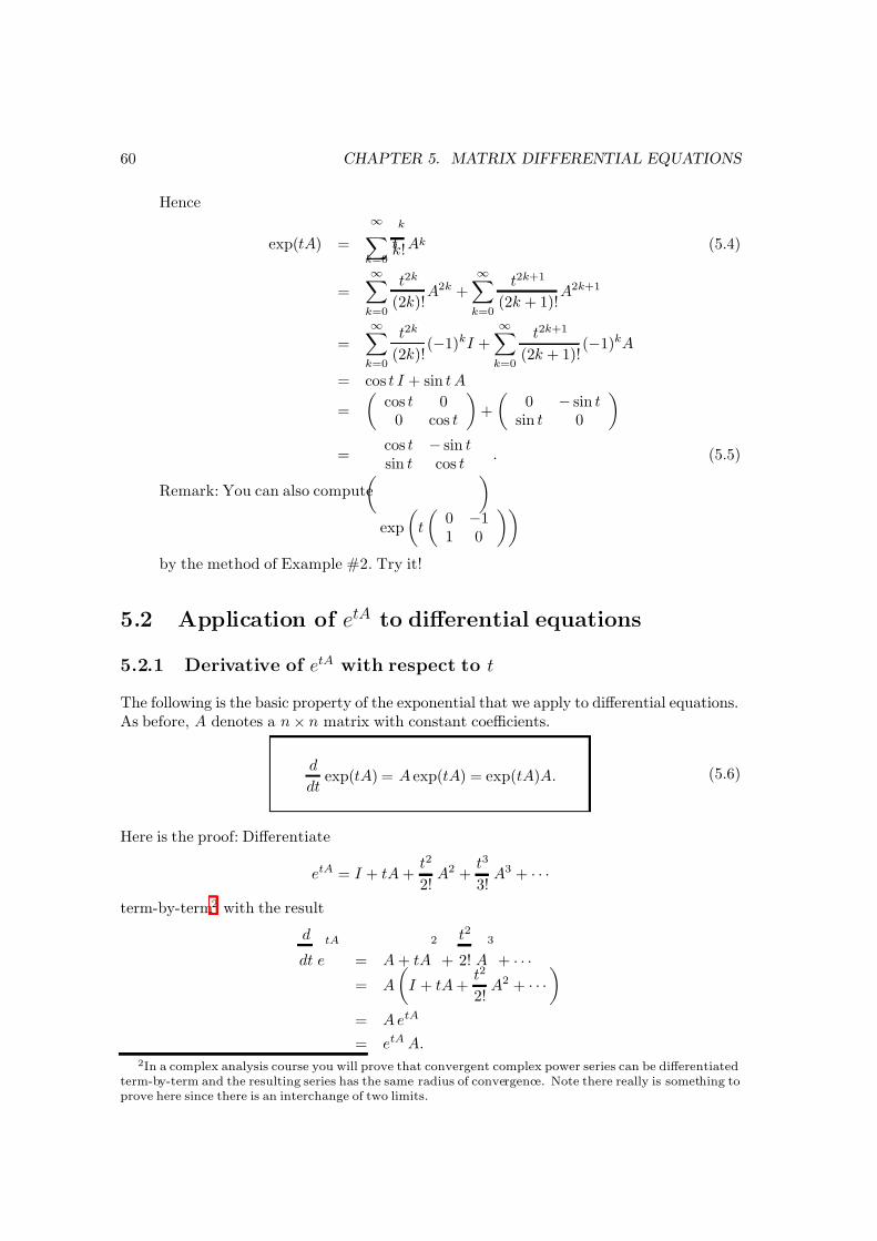
7/27/2019 22BBook.pdf



Hence

exp(tA) =

∞k=0

t

k

k! Ak (5.4)

=

∞k=0

t2k

(2k)!A2k +

∞k=0

t2k+1

(2k + 1)!A2k+1

=∞

k=0

t2k

(2k)!(−1)kI +

∞k=0

t2k+1

(2k + 1)!(−1)kA

= cos t I + sin t A

=

cos t 0

0 cos t

+

0 − sin t

sin t 0

= cos t − sin tsin t cos t . (5.5)

Remark: You can also compute

exp

t

0 −11 0

by the method of Example #2. Try it!

5.2 Application of etA to differential equations

5.2.1 Derivative of etA with respect to t

The following is the basic property of the exponential that we apply to differential equations.As before, A denotes a n × n matrix with constant coefficients.

d

dtexp(tA) = A exp(tA) = exp(tA)A. (5.6)

Here is the proof: Differentiate

etA = I + tA +t2

2!A2 +

t3

3!A3 + · · ·

term-by-term2 with the result

d

dt e

tA

= A + tA

2

+

t2

2! A

3

+ · · ·= A

I + tA +

t2

2!A2 + · · ·

= A etA

= etA A.2In a complex analysis course you will prove that convergent complex power series can be differentiated

term-by-term and the resulting series has the same radius of convergence. Note there really is something toprove here since there is an interchange of two limits.

7/27/2019 22BBook.pdf


5.2. APPLICATION OF MATRIX EXPONENTIAL TO DES 61

The last equality follows by factoring A out on the right instead of the left.

5.2.2 Solution to Matrix ODE with Constant Coefficients

We now use (5.6) to prove

Theorem: Letdx

dt= Ax (5.7)

where x ∈ Rn and A is a n × n matrix with constant coefficients. Then every solution of (5.7) is of the form

x(t) = exp(tA)x0 (5.8)

for some constant vector x0 ∈ Rn.

Proof : (i) First we show that x(t) = etAx0 is a solution:

dx

dt=

d

dt

etAx0

=

d

dtetA

x0

= AetAx0

= Ax(t).

(ii) We now show that every solution of (5.7) is of the form (5.8). Let y(t) by any solutionto (5.7). Let

∆(t) := e−tAy(t).

If we can show that ∆(t) is independent of t—that it is a constant vector which we call x0,

then we are done since multiplying both sides by etA shows

etAx0 = etA∆(t) = etAe−tAy(t) = y(t).

(We used the fact that tA and −tA commute so that the addition formula for the matrixexponential is valid.) To show that ∆(t) is independent of t we show its derivative withrespect to t is zero:

d∆

dt=

d

dte−tAy(t)

=

d

dte−tA

y(t) + e−tA dy

dt(chain rule)

= −e−tAA y(t) + e−tA (Ay(t)) (y(t) satisfies ODE)

= 0.

The next theorem relates the solution x(t) of (5.7) to the eigenvalues and eigenvectors of the matrix A (in the case A is diagonalizable).

Theorem: Let A be a diagonalizable matrix. Any solution to (5.7) can be written as

x(t) = c1etλ1ψ1 + c2etλ2ψ2 + · · · + cnetλnψn (5.9)

7/27/2019 22BBook.pdf



where λ1, . . . , λn are the eigenvalues of A with associated eigenvectors ψ1, . . . , ψn, andc1, . . . , cn are constants.

Proof : All solutions of (5.7) are of the form (5.8). Since A is diagonalizable, the eigen-vectors of A can be used to form a basis: ψ1, . . . , ψn. Since this is a basis there existconstants c1, . . . , cn such that

x0 = c1ψ1 + c2ψ2 + · · · + cnψn.

(x0 is the constant vector appearing in (5.8).)

For any eigenvector ψ of A with eigenvalue λ we have

etAψ = etλψ.

(This can be proved by applying the infinite series (5.2) to the eigenvector ψ and notingAkψ = λkψ for all positive integers k.) Thus

etAx0 = c1etAψ1 + · · · cnetAψn

= c1etλ1ψ1 + · · · + cnetλnψn.

Here are two immediate corollaries of this theorem:

1. If A is diagonalizable and has only real eigenvalues, then any solution x(t) of (5.1) willhave no oscillations.

2. If A is diagonalizable and the real part of every eigenvalue is negative, then

x(t) → 0 (zero vector), as t → +∞

To see this recall that if λ = σ + iµ (σ and µ both real), then

eλt = eσteiµt.

If σ < 0, eσt → 0 as t → +∞. Now apply preceding theorem.

Remarks: Here is an example using MatLab to solve a system of equations. Problem #9on page 421 of Boyce & DiPrima, 8th edition [4], asks us to find the general solution to

dx

dt = Ax

where A is given by (??). We computed in the above MatLab example the eigenvalues andeigenvectors (columns of V ) of A. Thus we can immediately write down the solution.

c1

1

−5/4−7/4

e−2t + c2

1

−4/3−2/3

e−t + c3

0

−11

e2t

7/27/2019 22BBook.pdf


5.3. RELATION TO EARLIER METHODS OF SOLVING CONSTANT COEFFICIENT DES 63

5.3 Relation to Earlier Methods of Solving Constant

Coefficient DEs

Earlier we showed how to solveay′′ + by′ + cy = 0

where a, b and c are constants. Indeed, we proved that the general solution is of the form

y(t) = c1etλ1 + c2etλ2

where λ1 and λ2 are the roots to

aλ2 + bλ + c = 0.

(We consider here only the case of distinct roots.)

Let’s analyze this familiar result using matrix methods. The x ∈ R2 is

x(t) =

x1x2

=

y

dy/dt

Therefore,

dx

dt=

dy/dt

d2y/dt2

=

x2

− ba

x2 − ca

x1

= 0 1

− ca − b

a

x1

x2

.

This last equality defines the 2 × 2 matrix A. The characteristic polynomial of A is

p(λ) = det(A − λI ) =

−λ 1− c

a − ba − λ

= λ2 +b

aλ +

c

a.

Thus the eigenvalues of A are the same quantities λ1 and λ2 appearing above. Since

x(t) = etAx0 = S

etλ1 0

0 etλ2

S −1x0,

x1(t) is a linear combination of etλ1 and etλ2 .

5.4 Inhomogenous Matrix Equations

Consider the inhomogenous equation

dx

dt= Ax + f (t), x(0) = x0 (5.10)

7/27/2019 22BBook.pdf



where x is a vector of dimension n, A a n× n constant coefficient matrix, and f (t) is a givenvector which in general depends upon the independent variable t. We use the method of

variation of parameters to find a particular solution to (5.10). Let3

x(t) = etAy(t)

Thendx

dt= AetAy(t) + etA dy

dt

To satisfy the differential equation this must equal

AetAy(t) + f (t)

and hence we must have

etA dy

dt= f (t)

Solving this for dy/dt:dy

dt= e−tAf (t)

The right hand side of the above equation is expressed in terms of known quantities. Inte-grating gives

y(t) =

t0

e−sAf (s) ds

and hence the particular solution

xpart(t) = etA

t0

e−sAf (s) ds

Thus the solution satisfying the initial condition is

x(t) = etA

t0

e−sAf (s) ds + etAx0 (5.11)

Observe that the solution of (5.10) has been reduced in (5.11) to matrix calculations andintegration.

5.5 Exercises

#1. Harmonic Oscillator via Matrix Exponentials

Write the oscillator equationx + ω2

0x = 0

as a first order system (5.1). (Explicitly find the matrix A.) Compute exp(tA) and showthat x(t) = exp(tA)x0 gives the now familiar solution. Note that we computed exp(tA) in(5.5) for the case ω0 = 1.

3If f (t) = 0 then we know that y(t) would be a constant vector. For nonzero f (t) we are allowing for thepossibility that y can depend upon t; hence the name variation of parameters.

7/27/2019 22BBook.pdf


5.5. EXERCISES 65

#2. Exponential of Nilpotent Matrices

1. Using the series expansion for the matrix exponential, compute exp(tN ) where

N =

0 10 0

.

Answer the same question for

N =

0 1 1

0 0 10 0 0

.

How do these answers differ from exp(tx) where x is any real number?

2. A n

×n matrix N is called nilpotent4 if there exists a positive integer k such that

N k = 0

where the 0 is the n × n zero matrix. If N is nilpotent let k be the smallest integersuch that N k = 0. Explain why exp(tN ) is a matrix whose entries are polynomials int of degree at most k − 1.

#3. Computing etA

Let

A =

1 −1 43 2 −12 1

−1

(5.12)

1. Find the eigenvalues and eigenvectors of A. (You can use any software package youlike and merely quote the results.)

2. Use these to compute etA.

#4.

Consider the system of linear differential equations

dx

dt= Ax

4In an advanced course in linear algebra, it will be proved that every matrix A can be written uniquely

as D + N where D is a diagonalizable matrix, N is a nilpotent matrix, and DN = ND . Furthermore, analgorithm will be given to find the matrices D and N from the matrix A. Once this is done then one cancompute exp(tA) as follows

exp(tA) = exp(tD + tN ) = exp(tD) exp(tN ).

We showed above how to reduce the computation of exp(tD), D a diagonalizable matrix, to linear algebra.This problem shows that exp(tN ) reduces to finitely many matrix multiplications. Thus the computation of both exp(tD) and exp(tN ) are reduced to linear algebra and hence so is exp(tA). Observe that it is crucialthat we know DN = ND .

7/27/2019 22BBook.pdf



where A is the 4 × 4 matrix

A =

−5/2 1 1/2 −1/23/4 −5/2 0 3/4

1 2 −3 10 2 −1/2 −2

(5.13)

Prove that all solutions x(t) to this DE tend to zero as t → ∞. Hint: You need not computeetA. You can prove this statement simply by computing the eigenvalues of A. (Why?)

#5.


dx

dt = Ax


A =

0 0 −3/2 2−3/4 1/2 0 −3/4

−1 −2 1 −11/2 −3 3/2 −3/2

(5.14)

Find a subspace V of R4 such that if x(0) ∈ V , then x(t) → 0 as t → ∞. Hint: The subspaceV is described in terms of (some of) the eigenvectors of A.

#6.


dx

dt= Ax


A =

1 α

−α 3

(5.15)

For what values of α will the solutions exhibit oscillatory behavior?

#7. Radioactive Decay & First Introduction to Laplace Transforms

Birth processes have been used since the time of Rutherford to model radioactive decay.(Radioactive decay occurs when an unstable isotope transforms to a more stable isotope,generally by emitting a subatomic particle.) In many cases a radioactive nuclide A decaysinto a nuclide B which is also radioactive; and hence, B decays into a nuclide C , etc.The nuclides B, C , etc. are called the progeny (formerly called daughters). This continuesuntil the decay chain reaches a stable nuclide. For example, uranium-238 decays throughα-emission to thorium-234 which in turn decays to protactinium-234 through β -emission.This chain continues until the stable nuclide lead-206 is reached.

http://nobelprize.org/nobel_prizes/chemistry/laureates/1908/

http://en.wikipedia.org/wiki/Alpha_decay


http://en.wikipedia.org/wiki/Beta_decay


http://www.ead.anl.gov/pub/doc/natural-decay-series.pdf

http://www.ead.anl.gov/pub/doc/natural-decay-series.pdf



http://nobelprize.org/nobel_prizes/chemistry/laureates/1908/

7/27/2019 22BBook.pdf


5.5. EXERCISES 67

1. Let the decay states be E 1 → E 2 → · · · → E N where E N is the final stable state. Wecan relabel these states to be simply 1, 2, . . . , N . (That is, we write E j as simply j.)

Let N (t) denote the state of the nuclide at time t. N (t) is a random process (calleda Markov process) due to the fact that radioactive decay is inherently random. Thuswe introduce

pj(t) = P( N (t) = j|N (0) = 1)

= probability that nuclide is in state j at time t

given it starts in state 1 at time t = 0.

These probabilities pj(t) satisfy differential equations called the Kolmogorov forward equations :

dpj

dt= λj−1 pj−1(t) − λj pj(t), j = 1, 2, . . . , N . (5.16)

The constants λj are called thedecay rates

. A decay rate λ is related to the half-life,T 1/2, of the nuclide by the well-known formula

T 1/2 =log2

λ, log 2 = 0.693147 . . . (5.17)

We assume λi = λj for i, j = 1, . . . , N − 1. We set λ0 = 0 and λN = 0. (λN is setequal to zero since the final state N is a stable nuclide and does not decay.)

In applications to radioactive decay, if N 1 is the number of initial nuclides (the thenumber of nuclides in state E 1), then N 1 pj(t) is the number of nuclides in state E j attime t.

2. Introduce the Laplace transform5

ˆ pj(s) = ∞0

e−ts pj(t) dt

and show that the Laplace transform of (5.16) is

sˆ pj(s) − δ j,1 = λj−1ˆ pj−1(s) − λj ˆ pj(s), j = 1, . . . , N . (5.18)

Solve these equations for ˆ pj(s) and show that

ˆ pj(s) =λ1

s + λ1

λ2

s + λ2· · · λj−1

s + λj−1

1

s + λj

3. Using the above expression for ˆ pj(s) partial fraction the result:

ˆ pj(s) =

jk=1

cj,k

s + λk

See if you can find expressions for cj,k. You might want to take some special cases tosee if you can make a guess for the cj,k. (The Mathematica command Apart willprove useful.)

5See Chapter 8 of these Notes and Boyce & Diprima, Chapter 6 [4].

http://en.wikipedia.org/wiki/Kolmogorov_equations



7/27/2019 22BBook.pdf



4. From the partial fraction decomposition of ˆ pj(s) explain why you can almost immedi-ately conclude

pj(t) =j

k=1

cj,k e−λkt, j = 1, 2, . . . , N . (5.19)

5. For the special case of N = 4: E 1 → E 2 → E 3 → E 4 find explicitly the proba-bilities pj(t). (You can use Mathematica if you wish. Note there is a commandInverseLaplaceTransform.)

6. Show that p2(t) has a maximum at t = tm

tm =log(λ1/λ2)

λ1 − λ2> 0.

In terms of the radioactive decay interpretation, this is the time when the first progeny

has a maximum population.

7. Using Mathematica (recall the command Series) show that as t → 0

p1(t) = 1 − λ1t + O(t2)

p2(t) = λ1t + O(t2)

p3(t) =1

2λ1λ2t2 + O(t3)

p4(t) =1

3!λ1λ2λ3t3 + O(t4)

8. Radon 222 gas is a chemically inert radioactive gas that is part of the Uranium 238decay chain. Radon and its radioactive progeny are known carcinogens. Here is part

of the decay chain6

· · ·−→ Rn 222 −→ Po 218 −→ Pb 214 −→ Bi 214 −→···

The half-life of each nuclide is known (recall (5.17)):

Rn 222: T 1/2 = 3.8235 days

Po 218: T 1/2 = 3.10 minutes

Pb 214: T 1/2 = 26.8 minutes

Bi 214: T 1/2 = 19.9 minutes

Let N Rn denote the initial amount of Rn 220 and assume the other nuclides are notpresent at time t = 0. Solve the Kolmogorov forward equations for this particular

birth process. (Note that here the probabilities do not sum to one since the Bi 214also decays.) This is not so messy if you use Mathematica. Find the times wheneach of the progeny have maximum population. (Highest probability) You might wantto use Mathematica’s FindRoot.

6Po=polonium, Pb=lead, Bi=bismuth.

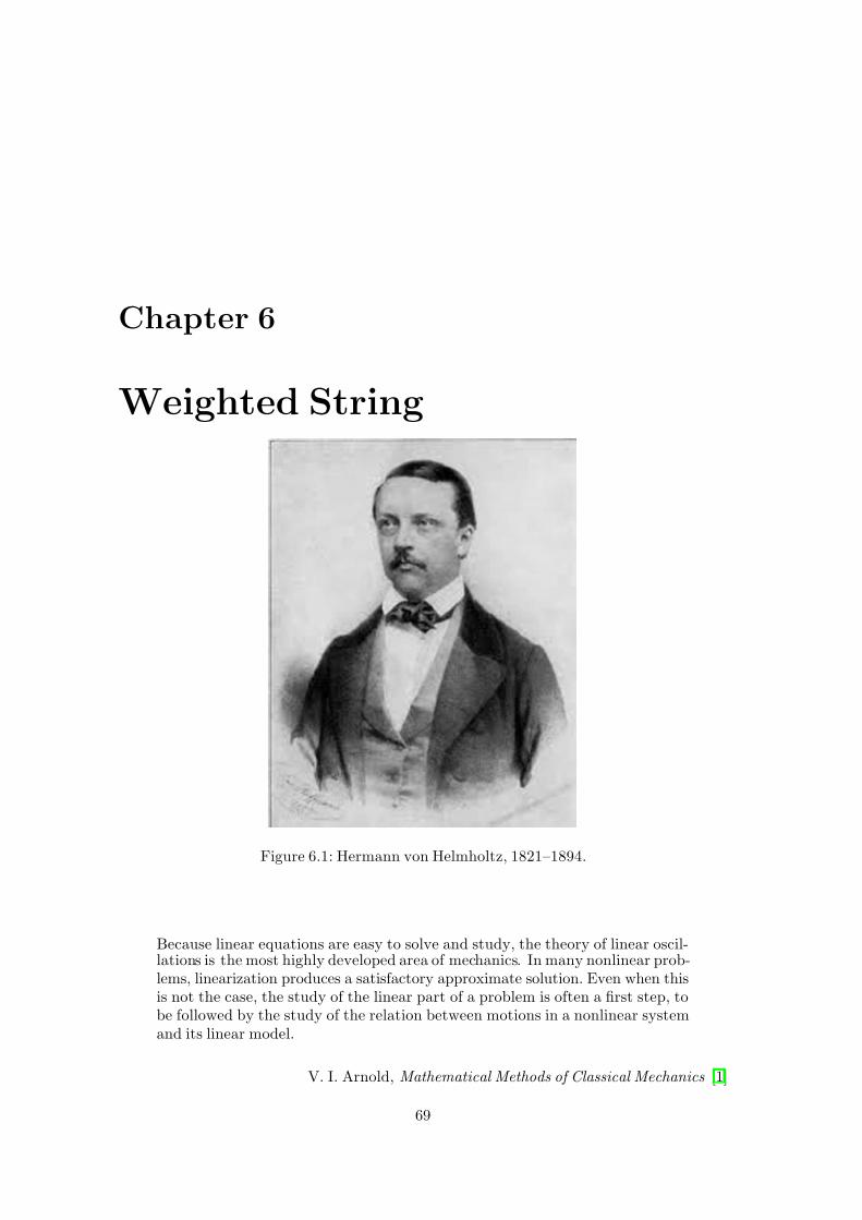
7/27/2019 22BBook.pdf


Chapter 6

Weighted String

Figure 6.1: Hermann von Helmholtz, 1821–1894.

Because linear equations are easy to solve and study, the theory of linear oscil-lations is the most highly developed area of mechanics. In many nonlinear prob-lems, linearization produces a satisfactory approximate solution. Even when thisis not the case, the study of the linear part of a problem is often a first step, tobe followed by the study of the relation between motions in a nonlinear systemand its linear model.

V. I. Arnold, Mathematical Methods of Classical Mechanics [1]

69

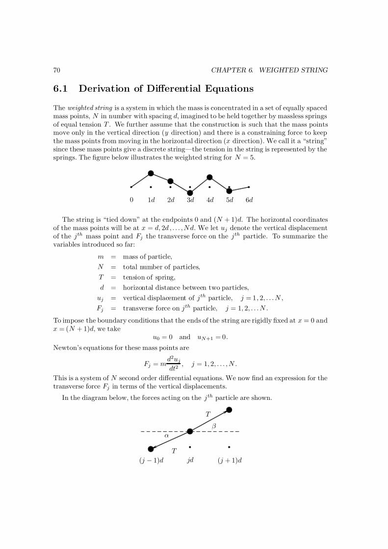
7/27/2019 22BBook.pdf


70 CHAPTER 6. WEIGHTED STRING

6.1 Derivation of Differential Equations

The weighted string is a system in which the mass is concentrated in a set of equally spacedmass points, N in number with spacing d, imagined to be held together by massless springsof equal tension T . We further assume that the construction is such that the mass pointsmove only in the vertical direction (y direction) and there is a constraining force to keepthe mass points from moving in the horizontal direction (x direction). We call it a “string”since these mass points give a discrete string—the tension in the string is represented by thesprings. The figure below illustrates the weighted string for N = 5.

0 1d 2d 3d 4d 5d 6d

The string is “tied down” at the endpoints 0 and (N + 1)d. The horizontal coordinatesof the mass points will be at x = d, 2d , . . . , N d. We let uj denote the vertical displacementof the jth mass point and F j the transverse force on the jth particle. To summarize thevariables introduced so far:

m = mass of particle,

N = total number of particles,

T = tension of spring,

d = horizontal distance between two particles,

uj = vertical displacement of jth particle, j = 1, 2, . . . N ,

F j = transverse force on jth particle, j = 1, 2, . . . N .

To impose the boundary conditions that the ends of the string are rigidly fixed at x = 0 andx = (N + 1)d, we take

u0 = 0 and uN +1 = 0.

Newton’s equations for these mass points are

F j = md2uj

dt2, j = 1, 2, . . . , N .

This is a system of N second order differential equations. We now find an expression for thetransverse force F j in terms of the vertical displacements.

In the diagram below, the forces acting on the jth particle are shown.

( j − 1)d jd ( j + 1)d

β

α

T

T

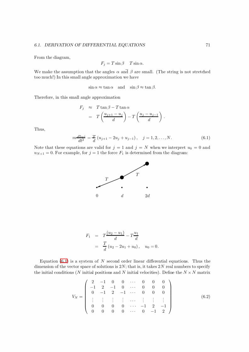
7/27/2019 22BBook.pdf


6.1. DERIVATION OF DIFFERENTIAL EQUATIONS 71

From the diagram,

F j = T sin β

−T sin α.

We make the assumption that the angles α and β are small. (The string is not stretchedtoo much!) In this small angle approximation we have

sin α ≈ tan α and sin β ≈ tan β.

Therefore, in this small angle approximation

F j ≈ T tan β − T tan α

= T

uj+1 − uj

d

− T

uj − uj−1

d

.

Thus,

m d2uj

dt2= T

d(uj+1 − 2uj + uj−1) , j = 1, 2, . . . , N . (6.1)

Note that these equations are valid for j = 1 and j = N when we interpret u0 = 0 anduN +1 = 0. For example, for j = 1 the force F 1 is determined from the diagram:

0 d 2d

T T

F 1 = T (u2 − u1)

d− T

u1

d

=T

d(u2 − 2u1 + u0) , u0 = 0.

Equation (6.1) is a system of N second order linear differential equations. Thus thedimension of the vector space of solutions is 2N ; that is, it takes 2N real numbers to specify

the initial conditions (N initial positions and N initial velocities). Define the N × N matrix

V N =

2 −1 0 0 · · · 0 0 0−1 2 −1 0 · · · 0 0 00 −1 2 −1 · · · 0 0 0...

......

... · · · ......

...0 0 0 0 · · · −1 2 −10 0 0 0 · · · 0 −1 2

(6.2)

7/27/2019 22BBook.pdf



and the column vector u

u =

u1

u2

··

uN

. (6.3)

Then (6.1) can be written in the compact matrix form

d2u

dt2+

T

mdV N u = 0. (6.4)

Note: We could also have written (6.1) as a first order matrix equation of the form

dx

dt= Ax (6.5)

where A would be a 2N × 2N matrix. However, for this application it is simpler to developa special theory for (6.4) rather than to apply the general theory of (6.5) since the matrixmanipulations with V N will be a bit clearer than they would be with A.

6.2 Reduction to an Eigenvalue Problem

Equation (6.4) is the matrix version of the harmonic oscillator equation

d2x

dt2+

k

mx = 0, ω2

0 =k

m. (6.6)

Indeed, we will show that (6.4) is precisely N harmonic oscillators (6.6)—once one choosesthe correct coordinates. We know that solutions to (6.6) are linear combinations of

cos ω0t and sin ω0t.

Thus we “guess” that solutions to (6.4) are linear combinations of the form

cos ωt f and sin ωt f

where ω is to be determined and f is a column vector of length N . (Such a “guess” can be

theoretically deduced from the theory of the matrix exponential when (6.4) is rewritten inthe form (6.5).)

Thus settingu = eiωtf ,

we see that (6.4) becomes the matrix equation

V N f =md

T ω2f .

7/27/2019 22BBook.pdf


6.3. COMPUTATION OF THE EIGENVALUES 73

That is, we must find the eigenvalues and eigenvectors of the matrix V N . Since V N is a realsymmetric matrix, it is diagonalizable with real eigenvalues. To each eigenvalue λn, i.e.

V N f n = λnf n, n = 1, 2, . . . , N ,

there will correspond a positive frequency

ω2n =

T

mdλn, n = 1, 2, . . . , N ,

and a solution of (6.4) of the form

un = (an cos(ωnt) + bn sin(ωnt)) f n

where an and bn are constants. This can now be easily verified by substituting this aboveexpression into the differential equation. To see we have enough constants of integration weobserve that we have two constants, an and bn, for each (vector) solution un. And we haveN vector solutions un—thus 2N constants in all. We now turn to an explicit evaluation of the frequencies ω2

n—such frequencies are called normal modes .

6.3 Computation of the Eigenvalues of V N

We introduce the characteristic polynomial of the matrix V N :

DN (λ) = DN = det (V N − λI ) .

Expanding the determinant DN in the last column, we see that it is a sum of two terms—each a determinant of matrices of size (N − 1) × (N − 1). One of these determinants equals

(2 − λ)DN −1 and the other equals DN −2 as is seen after expanding again, this time by thelast row. In this way one deduces

DN = (2 − λ)DN −1 − DN −2, N = 2, 3, 4, . . .

withD0 = 1 and D1 = 2 − λ.

We now proceed to solve this constant coefficient difference equation (in N ). From earlierwork we know that the general solution is of the form

c1µN 1 + c2µN

2

where µ1 and µ2 are the roots of

µ2 − (2 − λ)µ + 1 = 0.

Solving this quadratic equation gives

µ1,2 = 1 − λ

2± 1

2

(2 − λ)2 − 4 .

It will prove convenient to introduce an auxiliary variable θ through

2 − λ = 2 cos θ,

7/27/2019 22BBook.pdf



A simple computation now showsµ1,2 = e±iθ.

ThusDN = c1eiNθ + c2e−iNθ .

To determine c1 and c2 we require that

D0 = 1 and D1 = 2 − λ.

That is,

c1 + c2 = 1,

c1eiθ + c2e−iθ = 2 − λ = 2 cos θ.

Solving for c1 and c2,

c1 =eiθ

eiθ − e−iθ ,

c2 = − e−iθ

eiθ − e−iθ.

Therefore,

DN =1

eiθ − e−iθ

ei(N +1)θ − e−i(N +1)θ

=

sin((N + 1)θ)

sin θ.

The eigenvalues of V N are solutions to

DN (λ) = det(V N

−λI ) = 0.

Thus we requiresin((N + 1)θ) = 0,

which happens when

θ = θn :=nπ

N + 1, n = 1, 2, . . . , N .

Thus the eigenvalues of V N are

λn = 2 − 2cos θn = 4 sin2(θn/2), n = 1, 2, . . . , N . (6.7)

The eigenfrequencies are

ω2n =

T

mdλn =

2T

md(1 − cos θn)

= 2T md

1 − cos nπ

N + 1

= 4T

mdsin2

nπ2(N + 1)

. (6.8)

Remark: We know there are at most N distinct eigenvalues of V N . The index n doesnot start at zero because this would imply θ = 0, but θ = 0—due to the presence of sin θ in the denominator of DN —is not a zero of the determinant and hence does notcorrespond to an eigenvalue of V N . We conclude there are N distinct eigenvalues of V N .These eigenfrequencies are also called normal modes or characteristic oscillations .

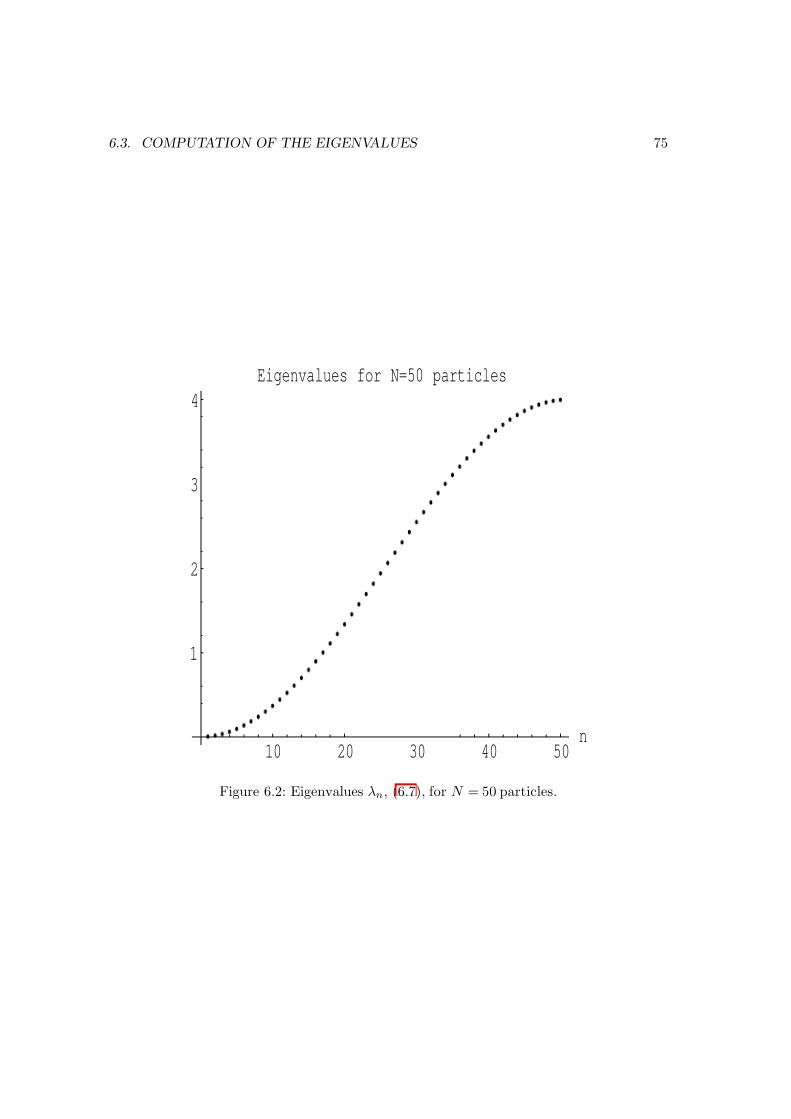
7/27/2019 22BBook.pdf


6.3. COMPUTATION OF THE EIGENVALUES 75

10 20 30 40 50n

1

2

3

4

Eigenvalues for N=50 particles

Figure 6.2: Eigenvalues λn, (6.7), for N = 50 particles.

7/27/2019 22BBook.pdf



6.4 The Eigenvectors

6.4.1 Constructing the Eigenvectors f n

We now find the eigenvector f n corresponding to eigenvalue λn. That is, we want a columnvector f n that satisfies

V N f n = 2(1 − cos θn)f n, n = 1, 2, . . . , N .

Setting,

f n =

f n1f n2··

f nN

,

the above equation in component form is

−f n,j−1 + 2f n,j − f n,j+1 = 2(1 − cos θn)f n,j

withf n,0 = f n,N +1 = 0.

This is a constant coefficient difference equation in the j index . Assume, therefore, a solutionof the form

f n,j = eijϕ.

The recursion relation becomes with this guess

−2cos ϕ + 2 = 2(1 − cos θn),

i.e.ϕ = ±θn.

The f n,j will be linear combinations of e±ijθn ,

f n,j = c1 sin( jθn) + c2 cos( jθn).

We require f n,0 = f n,N +1 = 0 which implies c2 = 0.

To summarize,

V N f n =md

T ω2

nf n, n = 1, 2, . . . , N ,

ω2n = 2T

md(1 − cos θn), θn = nπ

N + 1,

f n =

sin(θn)sin(2θn)

··

sin(N θn)

n = 1, 2, . . . , N .

(6.9)

7/27/2019 22BBook.pdf


6.5. DETERMINATION OF CONSTANTS 77

The general solution to (6.4) is

u(t) =N

n=1

(an cos(ωnt) + bn sin(ωnt)) f n,

or in component form,

uj(t) =N

n=1

(an cos(ωnt) + bn sin(ωnt)) sin( jθn). (6.10)

Thus every oscillation of the weighted string is a sum of characteristic oscillations.

6.4.2 Orthogonality of Eigenvectors

The set of eigenvectors f nN n=1 forms a basis for RN since the matrix V N is symmetric.

(Another reason they form a basis is that the eigenvalues of V N are distinct.) We claim theeigenvectors have the additional (nice) property that they are orthogonal, i.e.

f n · f m = 0, n = m,

where · denotes the vector dot product. The orthogonality is a direct result of the fact thatV N is a symmetric matrix. Another way to prove this is to use ( 6.9) to compute

f n · f m =N

j=1

sin( jθn)sin( jθm). (6.11)

To see that this is zero for n = m, we leave as an exercise to prove the trigonometric identity

N j=1

sin

njπ

N + 1

sin

mjπ

N + 1

=

1

2(N + 1)δ n,m

where δ n,m is the Kronecker delta function. (One way to prove this identity is first to usethe formula sin θ = (eiθ − e−iθ)/2i to rewrite the above sum as a sum of exponentials. Theresulting sums will be finite geometric series.) From this identity we also get that the lengthof each vector, f n, is

f n =

N + 1

2.

6.5 Determination of constants an and bn

Given the initial vectors u(0) and u(0), we now show how to determine the constants an

and bn. At t = 0,

u(0) =N

n=1

anf n.

7/27/2019 22BBook.pdf



Dotting the vector f p into both sides of this equation and using the orthogonality of theeigenvectors, we see that

a p =2

N + 1

N j=1

sin

pjπ

N + 1

uj(0), p = 1, 2, . . . , N . (6.12)

Differentiating u(t) with respect to t and then setting t = 0, we have

u(0) =n=1

ωnbnf n.

Likewise dotting f p into both sides of this equation results in

b p =2

N + 1

1

ω p

N

j=1

sinpjπ

N + 1 uj(0), p = 1, 2, . . . , N . (6.13)

If we assume the weighted string starts in an initial state where all the initial velocities arezero,

uj(0) = 0,

then the solution u(t) has components

uj(t) =N

n=1

an cos(ωnt)sin( jθn) (6.14)

where the constants an are given by (6.12) in terms of the initial displacements uj(0). Thespecial solutions obtained by setting all the an except for one to zero, are called the normal

modes of oscillation for the weighted string. They are most interesting to graph as a functionboth in space (the j index) and in time (the t variable). In figures we show a “snapshot” of

various normal mode solutions at various times t.

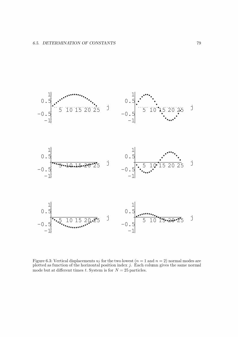
7/27/2019 22BBook.pdf


6.5. DETERMINATION OF CONSTANTS 79

5 10 15 20 25j

-1

-0.5

0.5

1

5 10 15 20 25j

-1

-0.5

0.5

1

5 10 15 20 25j

-1

-0.5

0.5

1

5 10 15 20 25j

-1

-0.5

0.5

1

5 10 15 20 25j

-1

-0.5

0.5

1

5 10 15 20 25j

-1

-0.5

0.5

1

Figure 6.3: Vertical displacements uj for the two lowest (n = 1 and n = 2) normal modes areplotted as function of the horizontal position index j. Each column gives the same normalmode but at different times t. System is for N = 25 particles.

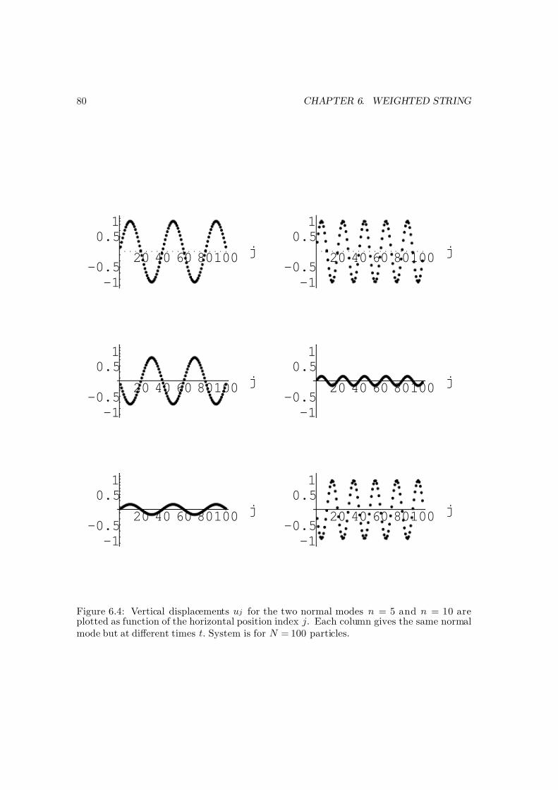
7/27/2019 22BBook.pdf



20 40 60 80100j

-1

-0.5

0.5

1

20 40 60 80100j

-1

-0.5

0.5

1

20 40 60 80100j

-1

-0.5

0.5

1

20 40 60 80100j

-1

-0.5

0.5

1

20 40 60 80100j

-1

-0.5

0.5

1

20 40 60 80100j

-1

-0.5

0.5

1

Figure 6.4: Vertical displacements uj for the two normal modes n = 5 and n = 10 areplotted as function of the horizontal position index j. Each column gives the same normalmode but at different times t. System is for N = 100 particles.

7/27/2019 22BBook.pdf


6.6. CONTINUUM LIMIT: THE WAVE EQUATION 81

6.6 Continuum Limit: The Wave Equation

As the pictures illustrate, when the number of particles N becomes large and the distance dbetween the particles becomes small, there appear limiting curves that describe the oscilla-tions of the entire system. These limiting curves describe the oscillations of the string. Letus pursue this in more detail. We assume

N → ∞ and d → 0 such that N d → L

where L is the length of the string (under no tension). We assume that the mass of thestring is given by µL where µ is the mass per unit length. Thus we assume

mN → µL

The positions of the particles, jd, j = 1, 2, . . . , N , are then assumed to approach a continuous

position variable x: jd → x

We now examine the continuum limit of the system of ordinary differential equations

d2uj

dt2=

T

md(uj−1 − 2uj + uj+1)

To do this we assume there exists a function u(x, t) such that

uj(t) = u( jd, t)

Then, since d is small,

uj−1 = u( jd − d, t) = u(x, t) − d ∂u∂x (x, t) + 12 d2 ∂

2

u∂x2 (x, t) + O(d3)

and similarly

uj+1 = u( jd + d, t) = u(x, t) + d∂u

∂x(x, t) +

1

2d2

∂ 2u

∂x2(x, t) + O(d3)

and hence

uj−1 − 2uj + uj+1 = d2∂ 2u

∂x2(x, t) + O(d3)

Substituting this into our differential equations we obtain

∂ 2u

∂t2

=T

µ

∂ 2u

∂x2

Note that since m = µL/N ,T d2

md=

T d

m=

T dN

µL=

T

µ

Also observe that T /µ has the dimensions of (velocity)2. Thus let’s call

v2 =T

µ

7/27/2019 22BBook.pdf



so that we have

∂ 2u∂x2

− 1v2

∂ 2u∂t2

= 0. (6.15)

This is the one-dimensional wave equation . It is an example of a partial differential equation .Given our analysis of the weighted string, we can anticipate that if we studied solutions of the single partial differential equation (6.15), then u = u(x, t) would describe the oscillationsof a string. Note that we would have the two boundary conditions

u(0, t) = u(L, t) = 0

which corresponds to the statement that the string is tied down at x = 0 and at x = L for alltimes t. In addition, we specify at t = 0 the initial displacement of the string: u(x, 0) = f (x)

where f is a given function as well as the initial velocity

∂u

∂t (x, 0). The problem then is tofind the solution to (6.15) satisfying these conditions. In the next section we show how themethods we’ve developed so far permit us to find such a solution.

6.6.1 Solution to the Wave Equation

We first look for solutions of the form (called separation of variables)

u(x, t) = X (x) T (t)

where X is only a function of x and T is only a function of t. Since

∂ 2u

∂x2 =d2X

dx2 T (t) and∂ 2u

∂t2 = X (x)d2T

dt2 ,

we have, upon substituting these expressions into (6.15) and dividing by X T the condition

1

X

d2X

dx2=

1

v21

T

d2T

dt2.

The left-hand side of the above equation is a function only of x and the right-hand side of the same equation is a function only of t. The only way this can be true is for both sides toequal the same constant. (We will see below that this constant has to be negative to satisfythe boundary conditions. Anticipating this fact we write the constant as −k2.) That is tosay, we have

1

X

d2X

dx2=

−k2 =

1

v2

1

T

d2T

dt2

This gives us two ordinary differential equations:

d2X

dx2+ k2X = 0,

d2T

dt2+ k2v2T = 0.

The solution to the first equation is

X (x) = c1 cos(kx) + c2 sin(kx).

7/27/2019 22BBook.pdf


6.6. CONTINUUM LIMIT: THE WAVE EQUATION 83

We want u(0, t) = 0 which implies c1 = 0. We also require u(L, t) = 0. If we set c2 = 0 thenX is identically zero and we have the trivial solution. Thus we must require

sin(kL) = 0.

This is satisfied if kL = nπ,n = 1, 2, 3, . . . .

(Note that n = −1, −2, . . . give the same solution up to a sign and n = 0 corresponds toX identically zero.) The solution to the T equation is also a linear combination of sinesand cosines. Thus for each value of n we have found a solution satisfying the conditionsu(0, t) = u(L, t) = 0 of the form

un(x, t) = sin(nπ

Lx)

an cos(nπv

Lt) + bn sin(

nπv

Lt)

where an and bn are constants. Since the wave equation is linear , linear supposition of solutions results in a solution. Thus

u(x, t) =∞

n=1

sin(nπ

Lx)

an cos(nπv

Lt) + bn sin(

nπv

Lt)

is a solution satisfying u(0, t) = u(L, t) = 0. We now require that u(x, 0) = f (x). That iswe want

u(x, 0) =∞

n=1

an sin(nπ

Lx) = f (x)

We now use the fact that

L0

sin(mπ

Lx)sin(

nπ

Lx) dx =

L

2δ m,n

to find

an =2

L

L0

f (x)sin(nπ

Lx) dx. (6.16)

This determines the constants an. If we further assume (for simplicity) that

∂u

∂t(x, 0) = 0

(initial velocity is zero), then a very similar calculation gives bn = 0. Thus we have shown

u(x, t) =∞

n=1

an sin(nπ

L

x) cos(nπv

L

t) (6.17)

where an are given by (6.16).

It is instructive to compare this solution of the wave equation to the solution ( 6.14) of the weighted string. We take the N → ∞ limit directly in (6.14) and use the same scalingas we have in the above derivation of the wave equation. In this limit we can replace

d −→ L

N , m −→ µL

N , j −→ xN

L

7/27/2019 22BBook.pdf



Thus

ω2

n=

4T

mdsin2(

nπ

2(N + 1))∼

4T

md

n2π2

4(N + 1)2 ∼T

µ

n2π2

L2

so thatωn −→ v

n π

L.

(Recall the definition v =

T /µ.) Similarly,

jθn =njπ

N + 1=

N

N + 1

nπ

Lx −→ nπ

Lx.

Putting these limiting expressions into (6.14) and taking the N → ∞ limit we see that (6.14)becomes (6.17). The only point that needs further checking is to show the an as given by(6.12) approaches the an as given by (6.16). This requires the natural assumption that theinitial conditions uj(0) can be written in the form uj(0) = f ( jd) for some smooth function

f . This is the f of u(x, 0) = f (x). A calculation then shows that (6.12) is the Riemann sumapproximation to (6.16) and approaches (6.16) as N → ∞.

The take home message is that the oscillations described by the solution to the waveequation can be equivalently viewed as an infinite system of harmonic oscillators.

6.7 Inhomogeneous Problem

The inhomogeneous version of (6.4) is

d2u

dt2+

T

mdV N u = F(t) (6.18)

where F(t) is a given driving term. The jth component of F(t) is the external force actingon the particle at site j. An interesting case of (6.18) is

F(t) = cos ωt f

where f is a constant vector. The general solution to (6.18) is the sum of a particularsolution and a solution to the homogeneous equation. For the particular solution we assumea solution of the form

u p(t) = cos ωt g.

Substituting this into the differential equation we find that g satisfies

V N

−

md

T

ω2I g =md

T

f .

For ω2 = ω2n, n = 1, 2, . . . , N , the matrix

V N − md

T ω2I

is invertible and hence

g =md

T

V N − md

T ω2I

−1f .

7/27/2019 22BBook.pdf


6.8. VIBRATING MEMBRANE 85

Writing (possible since the eigenvectors form a basis)

f =N

n=1

αnf n,

we conclude that

g =N

n=1

αn

ω2n − ω2

f n

for ω2 = ω2n, n = 1, 2, . . . , N . The solution with initial values

u(0) = 0, u(0) = 0 (6.19)

is therefore of the form

u(t) = cos ωtN

n=1

αn

ω2n − ω2

f n +n=1

(an cos(ωnt) + bn sin(ωnt)) f n .

Imposing the initial conditions (6.19) we obtain the two equations

n=1

αn

ω2n − ω2

+ an

f n = 0, (6.20)

n=1

ωnbnf n = 0. (6.21)

From the fact that f nN n=1 is a basis we conclude

an = −α

nω2

n − ω2 , bn = 0 for n = 1, 2, . . . , N .

Thus the solution is

u(t) =N

n=1

αn

ω2n − ω2

(cos(ωt) − cos(ωnt)) f n (6.22)

=N

n=1

2αn

ω2n − ω2

sin

1

2(ωn + ω)t

sin

1

2(ωn − ω)t

f n . (6.23)

We observe that there is a beat whenever the driving frequency ω is close to a normal modeof oscillation ωn. Compare this discussion with that of Boyce & DiPrima [4].

6.8 Vibrating Membrane

6.8.1 Helmholtz Equation

In the previous section we discussed the vibrating string. Recall that we have a string of unstretched length L that is tied down at ends 0 and L. If u = u(x; t) denotes the vertical

7/27/2019 22BBook.pdf



displacement of the string at position x, 0 ≤ x ≤ L, at time t, then we showed that for smalldisplacements u satisfies the one-dimensional wave equation

∂ 2u

∂x2− 1

v2∂ 2u

∂t2= 0

where v2 = T /µ, T equals the tension in string and µ is the density of the string. We solvedthis equation subject to the boundary conditions u(0, t) = u(L, t) = 0 for all t and withinitial conditions u(x, 0) = f (x) and ∂u

∂t (x, 0) = g(x) where f and g are given.

Now we imagine a uniform, flexible membrane, of mass ρ per unit area, stretched undera uniform tension T per unit length over a region Ω in the plane whose boundary ∂ Ω is asmooth curve (with a possible exception of a finite number of corners).

We now let U = U (x, y; t) denote the vertical displacement of the membrane at position(x, y)

∈Ω at time t from its equilibrium position. We again assume that the membrane is

tied down at the boundary; that is1

U (x, y; t) = 0 for (x, y) ∈ ∂ Ω.

The motion of U = U (x, y; t) is governed by the two-dimensional wave equation:

∂ 2U

∂x2+

∂ 2U

∂y2− 1

v2∂ 2U

∂t2= 0 for(x, y) ∈ Ω (6.24)

where v2 = T /ρ. One recognizes ∂ 2U ∂x2 + ∂ 2U

∂y2 as the two-dimensional Laplacian. So if we

introduce∆ =

∂

∂x2+

∂

∂y2

the wave equation takes the form

∆U − 1

v2∂ 2U

∂t2= 0.

We proceed as before an look for solutions of (6.24) in which the variables separate

U (x, y; t) = u(x, y)T (t).

Substituting this into (6.24), dividing by uT gives

1

u∆u =

1

v21

T

d2T

dt2.

The right-hand side depends only upon t where as the left-hand side depends only upon x, y.Thus for the two sides to be equal they must equal the same constant. Call this constant−k2. Thus we have the two equations

1In one dimension Ω = (0, L) and the boundary of Ω consists of the two points 0 and L.

7/27/2019 22BBook.pdf



d2T

dt2 + ω2

T = 0 where ω = kv,

∆u + k2u = 0. (6.25)

The differential equation for T has our well-known solutions

eiωt and e−iωt.

The second equation (6.25), called the Helmholtz equation , is a partial differential equationfor u = u(x, y). We wish to solve this subject to the boundary condition

u(x, y) = 0 for (x, y) ∈ ∂ Ω.

6.8.2 Rectangular Membrane

Consider the rectangular domain

Ω = (x, y) : 0 < x < a, 0 < y < b (6.26)

For this rectangular domain the Helmholtz equation can be solved by the method of sepa-ration of variables. If one assumes a solution of the form (variables x and y separate)

u(x, y) = X (x)Y (y)

then the problem is reduced to two one-dimensional problems. It is an exercise to show thatthe allowed frequencies are

ωm,n = πv

m

a

2+n

b

21/2, m , n = 1, 2, 3, . . . (6.27)

6.8.3 Circular Membrane: The Drum

We now consider the circular domain

Ω =

(x, y) : x2 + y2 < a2

so the boundary of Ω is the circle ∂ Ω : x2 + y2 = a2. Even though the variables separate inthe Cartesian coordinates x and y, this is of no use since the boundary is circular and wewould not be able to apply the BC u = 0 on the circular boundary ∂ Ω. Since the domain iscircular it is natural to introduce polar coordinates

x = r cos θ, y = r sin θ.

It is an exercise in the chain rule to show that in polar coordinates the 2D Laplacian is

∆u =∂ 2u

∂r2 +1

r

∂u

∂r +1

r2∂ 2u

∂θ2 ;

and hence, the Helmholtz equation in polar coodinates is

∂ 2u

∂r2+

1

r

∂u

∂r+

1

r2∂ 2u

∂θ2+ k2u = 0. (6.28)

We write u = u(r, θ).2

2Possible point of confusion: We wrote u = u(x, y) so really our new function of r and θ is u(r cos θ, r sin θ).Technically we should give this function of r and θ a new name but that would be rather pedantic.

7/27/2019 22BBook.pdf



Separation of Variables

We now show that the variables separate. So we look for a solution of the form

u(r, θ) = R(r)Θ(θ).

Substituting this into (6.28), multiplying by r2/RΘ we have

r2

R

d2R

dr2+

r

R

dR

dr+ k2r2 = − 1

Θ

d2Θ

dθ2

By the now familiar argument we see that each of the above sides must equal a constant,call it m2, to obtain the two differential equations

d2Θ

dθ2+ m2Θ = 0 (6.29)

d2Rdr2

+ 1r

dRdr

+ (k2 − m2

r2)R = 0 (6.30)

Two linearly independent solutions to (6.29) are

eimθ and e−imθ

The point with polar coordinates (r, θ) is the same point as the one with polar coordinates(r, θ + 2π). Thus our solution u(r, θ) and u(r, θ + 2π) must be the same solution. Thisrequires

eimθ+im2π = eimθ

or e2πim = 1. That is, m must be an integer. If m = 0 the general solution to (6.29) isc1 + c2θ. But the θ → θ + 2π argument requires we take c2 = 0. Thus the general solution

to (6.29) is am cos(mθ) + bm sin(mθ), m = 0, 1, 2, . . .

We now return to (6.30), called the Bessel equation , which is a second order linear differentialequation. General theory tells us there are two linearly independent solutions. Tradition hasit we single out two solutions. One solution, called J m(kr), is finite as r → 0 and the othersolution, called Y m(kr) goes to infinity as r → 0. Both of these functions are called Bessel

functions . It can be shown that the Bessel function J m(z) is given by the series expansion

J m(z) =z

2

m ∞j=0

(−1)j1

j!(m + j)!

z

2

2j(6.31)

A plot of the Bessel function J 0(x) for 0 ≤ x ≤ 40 is given in Figure 6.5. In Mathematica,Bessel functions J m(z) are called by the command BesselJ[m,z]. Since u(r, θ) is well-defined at r = 0 (center of the drum), this requires we only use the J m solutions. Thus wehave shown that

J m(kr) (am cos(mθ) + bm sin(mθ)) , m = 0, 1, 2, . . .

are solutions to (6.28). We now require that these solutions vanish on ∂ Ω. That is, whenr = a and for all θ we require the above solution to vanish. This will happen if

J m(ka) = 0.

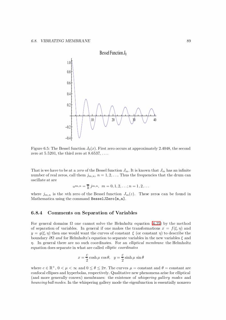
7/27/2019 22BBook.pdf



10 20 30 40

0.4

0.2

0.2

0.4

0.6

0.8

1.0

Bessel Function J 0

Figure 6.5: The Bessel function J 0(x). First zero occurs at approximately 2.4048, the secondzero at 5.5201, the third zero at 8.6537, . . . .

That is we have to be at a zero of the Bessel function J m. It is known that J m has an infinitenumber of real zeros, call them jm,n, n = 1, 2, . . .. Thus the frequencies that the drum canoscillate at are

ωm,n = va jm,n, m = 0, 1, 2, . . . ; n = 1, 2, . . .

where jm,n is the nth zero of the Bessel function J m(z). These zeros can be found inMathematica using the command BesselJZero[m,n].

6.8.4 Comments on Separation of Variables

For general domains Ω one cannot solve the Helmholtz equation (6.25) by the methodof separation of variables. In general if one makes the transformations x = f (ξ, η) andy = g(ξ, η) then one would want the curves of constant ξ (or constant η) to describe theboundary ∂ Ω and for Helmholtz’s equation to separate variables in the new variables ξ andη. In general there are no such coordinates. For an elliptical membrane the Helmholtzequation does separate in what are called elliptic coordinates

x =c

2cosh µ cos θ, y =

c

2sinh µ sin θ

where c ∈ R+, 0 < µ < ∞ and 0 ≤ θ ≤ 2π. The curves µ = constant and θ = constant are

confocal ellipses and hyperbolas, respectively. Qualitative new phenomena arise for elliptical(and more generally convex) membranes: the existence of whispering gal lery modes andbouncing ball modes . In the whispering gallery mode the eigenfunction is essentially nonzero

7/27/2019 22BBook.pdf



only in a thin strip adjacent to the boundary of Ω. Thus a person who speaks near the wallof a convex room can be heard across the room near the wall, but not in the interior of the

room. For further information see [5] and references therein.

6.9 Exercises

#1. Weighted String on a Circle

We consider the same weighted string problem but now assume the masses lie on a circle;this means that the first mass is coupled to the last mass by a string. The effect of thisis that (6.1) remains the same if we now interpret u0 = uN and uN +1 = u1. Explain whythis is the case. What is the matrix V N in this case? Show that the differential equationscan still be written in the matrix form (6.4) where now the V N is your new V N . Does the

reduction to an eigenvalue problem, as in §6.2, remain the same? Explain.

#2. Diagonalization of V N from Problem #1

Let V N be the N × N matrix found in the previous problem. Show that the eigenvalueproblem

V N f = λf

becomes in component form

−f j−1 + 2f j − f j+1 = λf j , j = 1, 2, . . . , N (6.32)

where f 0 = f N and f N +1 = f 1. Let ω denote an N th root of unity; that is, any of the values

e2πin/N , n = 0, 1, . . . , N − 1. For each such choice of ω, define

f ω =

N j=1

f j ωj (6.33)

Multiply (6.32) by ωj and sum the resulting equation over j = 1, 2, . . . , N . Show that theresult is

2(1 − cos φ)f ω = λf ω

where ω = eiφ. From this we conclude that the eigenvalues are

λn = 2

1 − cos

2πn

N , n = 0, 1, . . . , N − 1

Explain why this is so. This should be compared with (6.7). Find an eigenvector f n corre-sponding to eigenvalue λn. (Hint: Follow the method in §6.4.1.)

#3. Coupled Pendulums

Consider the system of two mathematical pendulums of lengths ℓ1 and ℓ2 and masses m1

and m2, respectively, in a gravitional field mg which move in two parallel vertical planes

7/27/2019 22BBook.pdf


6.9. EXERCISES 91

perpendicular to a common flexible support such as a string from which they are suspended.Denote by θ1 (θ2) the angle of deflection of pendulum #1 (#2). The kinetic energy of this

system is

KE =1

2m1ℓ21θ21 +

1

2m2ℓ22θ22 ,

and the potential energy is

PE = m1g ℓ1(1 − cos θ1) + m2g ℓ2(1 − cos θ2) + V int

where V int is the interaction potential energy.3 If there is no twist of the support, then thereis no interaction of the two pendulums. We also expect the amount of twist to depend uponthe difference of the angles θ1 and θ2. It is reasonable to assume V int to be an even functionof θ1 − θ2. Thus

V int(0) = 0, V ′int(0) = 0.

For small deflection angles (the only case we consider) the simplest assumption is then to

takeV int(θ1 − θ2) =

1

2κ(θ1 − θ2)2

where κ is a positive constant. Since we are assuming the angles are small, the potentialenergy is then given, to a good approximation, by

PE =1

2m1gℓ1 θ21 +

1

2m2gℓ2 θ22 +

1

2κ(θ1 − θ2)2.

Under these assumptions it can be shown that Newton’s equations are

m1ℓ21θ1 = −(m1gℓ1 + κ)θ1 + κθ2 ,

m2ℓ22θ2 = κθ1 − (m2gℓ2 + κ)θ2 .

Observe that for κ = 0 the ODEs reduce to two uncoupled equations for the linearized

mathematical pendulum. To simplify matters somewhat, we introduce

ω21 =

g

ℓ1, ω2 =

g

ℓ2k1 =

κ

m1ℓ21, k2 =

κ

m2ℓ22.

Then it is not difficult to show (you need not do this) that the above differential equationsbecome

θ1 = −(ω21 + k1)θ1 + k1θ2

θ2 = k2θ1 − (ω22 + k2)θ2 .

(6.34)

We could change this into a system of first order DEs (the matrix A would be 4 × 4).However, since equations of this form come up frequently in the theory of small oscillations,we proceed to develop a “mini theory” for these equations. Define

Θ =

θ1θ2

.

3These expressions should be compared with (2.25).

7/27/2019 22BBook.pdf



Show that the equations (6.34) can be written as

Θ = AΘ (6.35)

where A is a 2 × 2 matrix. Find the matrix A. Assume a solution of (6.35) to be of the form

Θ(t) = eiωt

a1a2

. (6.36)

Using (6.36) in (6.35) show that (6.35) reduces to

AΘ = −ω2Θ. (6.37)

This is an eigenvalue problem. Show that ω2 must equal

ω2± =

1

2(ω2

1 + ω22 + k1 + k2)

±1

2

(ω2

1 − ω22)2 + 2(ω2

1 − ω22)(k1 − k2) + (k1 + k2)2 . (6.38)

Show that an eigenvector for ω2+ is

f 1 =

1

−k2(ω2+ − ω2

2 − k2)−1

, (6.39)

and an eigenvector corresponding to ω2− is

f 2 =

−k1(ω2− − ω2

1 − k1)−1

1

. (6.40)

Now show that the general solution to (6.34) isθ1(t)θ2(t)

= (c1 cos(ω+t) + c2 sin(ω+t)) f 1 + (c3 cos(ω−t) + c4 sin(ω−t)) f 2 (6.41)

where ci are real constants. One can determine these constants in terms of the initial data

θ1(0), θ1(0), θ2(0), θ2(0).

To get some feeling for these rather complicated expressions, we consider the special case

θ1(0) = θ0, θ1(0) = 0, θ2(0) = 0, θ2(0) = 0 (6.42)

with

m1 = m2 = m, ℓ1 = ℓ2 = ℓ. (6.43)These last conditions imply

ω1 = ω2 := ω0.

Explain in words what these initial conditions, (6.42), correspond to in the physical setup.

If we definek =

κ

m ℓ2,

7/27/2019 22BBook.pdf


6.9. EXERCISES 93

show that in the special case (6.42) and (6.43) that

ω+ =

ω20 + 2k and ω− = ω0. (6.44)

In this same case solve for the coefficients c1, c2, c3 and c4 and show that

c1 =1

2θ0, c2 = 0, c3 =

1

2θ0, c4 = 0,

and hence (6.41) becomes

θ1(t) = θ0 cos

1

2(ω+ + ω−)t

cos

1

2(ω+ − ω−)t

,

θ2(t) = θ0 sin1

2(ω+ + ω−)t sin

1

2(ω+ − ω−)t .

Suppose further thatk

ω20

≪ 1. (6.45)

What does this correspond to physically? Under assumption (6.45), show that approximately

θ1(t) ≈ θ0 cos(ω0t) cos

k

2ω0t

,

θ2(t) ≈ θ0 sin(ω0t) sin

k

2ω0t

. (6.46)

Discuss the implications of (6.46) in terms of the periods

T 0 =2π

ω0and T 1 =

2π

k/2ω0.

Show that in this approximationT 1 ≫ T 0.

Draw plots of θ1(t) and θ2(t) using the approximate expressions (6.46).

#4. The Toda Chain and Lax Pairs

Consider N particles on a circle (periodic boundary conditions) whose positions xn(t) at

time t satisfy the Toda equations

d2xn

dt2= exp (−(xn − xn−1)) − exp(−(xn+1 − xn)) , n = 1, 2, . . . , N , (6.47)

where xN +1 = x1 and x0 = xN . These equations are nonlinear and admit certain solutions,called solitons , which are stable pulses. This system of equations has been extensivelystudied. Here we give only a brief introduction to some of these results. 4

4See, for example, Theory of Nonlinear Lattices by Morikazu Toda, Springer-Verlag, 1981.

7/27/2019 22BBook.pdf



To make the problem easier we now set N = 5 but everything that follows can begeneralized to any positive integer N .

Define

an =1

2exp(−(xn+1 − xn)/2) and bn =

1

2

dxn

dt, n = 1, . . . , 5. (6.48)

Show that if xn satisfies the Toda equations (6.47), then an and bn satisfy the differentialequations

dan

dt= an (bn − bn+1) and

dbn

dt= 2

a2n−1 − a2n

. (6.49)

Define two 5 × 5 matrices L and B, they are called a Lax pair , by

L =

b1 a1 0 0 a5a1 b2 a2 0 00 a2 b3 a3 0

0 0 a3 b4 a4a5 0 0 a4 b5

and B =

0 −a1 0 0 a5

a1 0 −a2 0 00 a2 0 −a3 0

0 0 a3 0 −a4−a5 0 0 a4 0

. (6.50)

Show (6.49) can be written as the matrix equation

dL

dt= BL − LB (6.51)

Define the matrix U = U (t) to be the solution to the differential equation

dU

dt= BU

that satisfies the initial condition U (0) = I .

Show that U (t) is a unitary matrix; that is, U ∗(t)U (t) = I for all t where U ∗ is theadjoint matrix.5 Hint: Observe that B∗ = −B. Use this to first show that

dU ∗

dt= −U ∗B

and then show ddtU ∗(t)U (t) = 0.

Now prove thatd

dt(U ∗L(t)U (t)) = 0

and hence thatU ∗(t)L(t)U (t) = L(0)

That is, L(0) and L(t) are unitarily equivalent. From this conclude

The eigenvalues of L(t) are independent of t

Thus the eigenvalues of the Lax matrix L are first integrals of motion of the Toda chain. Forgeneral N this means that we have found N integrals of the motion. This is a remarkableresult since normally one can only find a limited number of integrals of the motion (energy,angular momentum, etc.).

5Recall that if X is any matrix then X ∗ is the matrix obtained by taking the complex conjugate of eachelement in X and then taking the transpose.

7/27/2019 22BBook.pdf


6.9. EXERCISES 95

#5. Wave equation

In the section “Solution to the Wave Equation” it was claimed that a similar argumentshows that the coefficients bn are equal to zero. (See discussion between (6.16) and (6.17).)Prove that bn = 0.

#6. Weighted String with Friction

We now assume that the particles in the weighted string problem are subject to a force dueto the presence of friction. (Imagine the particles are moving in a medium which offersresistance to the motion of the particles.) Assuming the frictional force is proportional tothe velocity, the system of differential equations describing the motion is

md2uj

dt2 =T

d (uj+1 − 2uj + uj−1) − γ duj

dt , j = 1, 2, . . . , N (6.52)

where γ is positive and, as before, u0 = uN +1 = 0.

1. Rewrite the system (6.52) in matrix form such that when γ = 0 the equation becomesidentical to the matrix equation (6.4).

2. Assume a solution of the form

u(t) = eiωtf (6.53)

where f is a column vector independent of t and ω is to be determined. For whatvalues of ω is (6.53) a solution to the matrix equation derived in part (1)?

Note:

This will not require acomplete

reworking of the eigenvalues since you may usethe information we already have proved about V N to find the eigenvalues in this newproblem. You should not have to solve anything more complicated than a quadraticequation.

3. Explain the significance of the fact that the ω’s you obtain are complex numbers.

4. For a large system N ≫ 1 explain why you expect some of the allowed ω’s to be purely

imaginary . Explain the significance of this result, i.e. what is the implication for themotion?

#7. Rectangular Membrane

In this section we obtain the solution of (6.25) in the case of a rectangular domain (6.26).

1. By assuming that the solution can be written as u(x, y) = X (x)Y (y), obtain a 2ndorder DE for X with independent variable x and similarly a DE for Y with independentvariable y.

2. We assume the membrane is tied down at the boundary of the domain Ω. (This impliesboundary conditions on the solutions we seek.)

7/27/2019 22BBook.pdf



3. Show that the eigenvalues and the corresponding eigenfunctions of the differentialequations with boundary conditions in parts (1) and (2) are

µm =m2π2

a2; X m(x) = Am sin

mπx

a

, m = 1, 2, · · · (6.54)

ν n =n2π2

b2; Y n(y) = Bn sin

nπy

b

, n = 1, 2, · · · (6.55)

4. Show that the eigenfrequencies (normal modes) of the rectangular membrane are givenby (6.27). (By dimensional analysis conclude where the factor v, which was set equalto one here, must appear.)

5. Find the general solution to (6.25) for this rectangular domain.

#8. Alternating Mass-Spring: Acoustic and Optical Phonons

Consider 2N particles on a circle interacting via a spring connnecting adjacent particles.We assume the particles on the odd sites have mass m1 and the particles on the even siteshave mass m2. If uj denotes the displacement from equilibrium of particle j, the differentialequations describing the motion are

mjd2uj

dt2+ k (−uj−1 + 2uj − uj+1) = 0 for j = 1, 2, 3, . . . , 2N, (6.56)

where because the particles are on a circle

u2N +1 = u1 and u0 = u2N .

Here k is the spring constant for the spring connecting any two particles. We are interestedin finding the frequencies at which the system can oscillate.

1. Assume a solution of the form

uj(t) = eiωtvj , vj independent of t,

and show that (6.56) becomes

−mjω2vj + k (−vj−1 + 2vj − vj+1) = 0 for j = 1, 2, 3, . . . , 2N, (6.57)

2. For j = 1, 2, . . . , N define the vectors

V j =

v2j−1v2j

.

Show that (6.57) can be written equivalently as

−

m1 00 m2

ω2V j +k

−

0 10 0

V j−1 +

2 −1

−1 2

V j −

0 01 0

V j+1

= 0

(6.58)for j = 1, 2, . . . , N .

7/27/2019 22BBook.pdf


6.9. EXERCISES 97

3. Let η denote any N th root of unity, i.e. ηN = 1 so η is of the form η = eiφ = e2πij/N

for some integer j = 0, 1, . . . , N

−1. Define

V η =N

j=1

V jηj

Show that V η satisfies the equation−

m1 00 m2

ω2 + k

−

0 10 0

η +

2 −1

−1 2

−

0 01 0

η−1

V η = 0.

(6.59)

4. What is the condition for nontrivial solutions V η to exist for (6.59)? Hint: Equation

(6.59) is of the form AV η = 0 where the matrix A is the 2 × 2 matrix inside the curlybrackets of (6.59). Using the condition you just found, show that the normal modesof vibration are given by

ω2±,j = k

1

m1+

1

m2

± k

1

m21

+1

m22

+2

m1m2cos

2πj

N

1/2(6.60)

where j = 0, 1, 2, . . . N − 1.

5. Show that the frequencies derived in (6.60) lie on two curves, called dispersion curves .These two curves should be compared with the one dispersion curve for the equal massproblem. Plot the two dispersion curves.6 The curve that is zero at j = 0 is calledthe acoustic mode and the other is called the optical mode .7 This is a model of aone-dimensional lattice vibrations of a diatomic system.

#9. Energy of the Vibrating String

The vibrating string has the total energy E (t) at time t

E (t) =

L0

1

2µ u2

t (x, t) +1

2T u2

x(x, t)

dx

Explain why the first term is the kinetic energy and the second term is the potential energyof the vibrating string. Recall the solution u(x, t) of the vibrating string problem, i.e. (6.17).Above we use the notation

ut(x, t) :=∂u(x, t)

∂tand ux(x, t) :=

∂u(x, t)

∂x.

You may assume as given the following integrals: L0

sinmπ

Lx

sinnπ

Lx

dx =1

2L δ m,n (6.61)

6In plotting you might want to fix some values of m1, m2 and k.7The acoustic modes correspond to sound waves in the lattice. The optical modes, which are nonzero at

j = 0, are called “optical” because in ionic crystals they are excited by light. The quantized version of theseexcitations are called acoustic phonons and optical phonons.

7/27/2019 22BBook.pdf



and

L0 cos

mπ

L x

cosnπ

L x

dx =

1

2 L δ m,n (6.62)

Use (6.61) and (6.62) to show

E (t) =π2T

4L

∞n=1

n2a2n. (6.63)

Note that the result is independent of t, i.e. the energy of the vibrating string is conserved.Give a physical interpretation of this expression for E in terms of harmonic oscillators.

7/27/2019 22BBook.pdf


Chapter 7

Quantum Harmonic Oscillator

Figure 7.1: Erwin Schrodinger, 1887–1961 and Paul Dirac, 1902–1984.

A simple and interesting example of a dynamical system in quantum mechanicsis the harmonic oscillator. This example is of importance for general theory,

because it forms a corner-stone in the theory of radiation.

P. A. M. Dirac, The Principles of Quantum Mechanics

99

7/27/2019 22BBook.pdf


100 CHAPTER 7. QUANTUM HARMONIC OSCILLATOR

7.1 Schrodinger Equation

In classical mechanics the state of a system consisting of N particles is specified by theposition x and momentum p = mv of each particle. The time evolution of this state is de-termined by solving Newton’s Second Law (or equivalently, say Hamilton’s equations). Thus,for example, a one particle system moving in three-dimensions (three degrees of freedom)determines a curve in 6-dimensional space: namely, ( x(t), p(t)). For the familiar harmonicoscillator (mass-spring system) there is only one-degree of freedom (the movement of themass is in one dimension only) and the position and momentum are given by the now familiarformulas1

x(t) = x0 cos(ω0t) +p0

mω0sin(ω0t), (7.1)

p(t) = p0 cos(ω0t) − mω0x0 sin(ω0t). (7.2)

In quantum mechanics the notion of the state of the system is more abstract. The stateis specified by a vector Ψ in some abstract vector space H. This vector space has an innerproduct (·, ·).2 Thus every state Ψ ∈ H satisfies

Ψ := (Ψ, Ψ)1/2 < ∞. (7.3)

The importance of (7.3) is that in the Born interpretation |(Ψ, Φ)|2 is interpreted as aprobability; and hence, must be finite (and less than or equal to one).3 In what is called theSchrodinger representation, one can describe the state Ψ as a function Ψ(x) where x is theposition (of say the particle). Then

|Ψ(x)

|2 is the probability density of finding the particle

in some small neighborhood of the point x. Integrating this over all possible positions mustthen give one.

The evolution of the state Ψ with time is determined by solving the Schrodinger equation:

i ∂ Ψ

∂t= H Ψ. (7.4)

Here is the Planck’s constant4 (divided by 2π) and H is the quantum mechanical Hamil-tonian, a linear self-adjoint operator on the space H.5

1

Actually, the second may look a little different from the earlier formulas. This is due to the fact thatwe are using momentum p instead of velocity v to describe the second coordinate of (x, p). Here p0 is theinitial momentum and is related to the initial velocity by p0 = mv0.

2Such vector spaces are called Hilbert spaces.3This assumes that states Ψ are normalized so that their “length” is one, i.e. Ψ = 1.4In the cgs system, = 1.05457 × 10−27 erg-sec. A quantity that has the units of energy×time is called

an action . In modern particle physics a unit system is adopted such that in these units = 1. Max Planckreceived the Nobel prize in 1919 for “his discovery of energy quanta”.

5An operator H is self-adjoint if (Hψ ,ψ) = (ψ ,Hψ) for all ψ ∈ H. It is the generalization to Hilbertspaces of the notion of a Hermitian matrix. There are some additional subtle questions regarding the domainof the operator H . In these notes we ignore such questions and assume H is well-defined on all states Ψ ∈ H.

http://nobelprize.org/nobel_prizes/physics/laureates/1933/schrodinger.html


http://en.wikipedia.org/wiki/Planck_constant

http://nobelprize.org/nobel_prizes/physics/laureates/1918/planck.html

http://nobelprize.org/nobel_prizes/physics/laureates/1918/planck.html

http://en.wikipedia.org/wiki/Planck_constant


7/27/2019 22BBook.pdf


7.2. HARMONIC OSCILLATOR 101

7.2 Harmonic Oscillator

7.2.1 Harmonic Oscillator Equation

We illustrate the notions of quantum mechanics and its relationship to differential equationsin the context of the harmonic oscillator. The harmonic oscillator is one of the most impor-tant simple examples in quantum mechanics. In this case the vector space H is the space of square-integrable functions. This space consists of all (complex valued) functions ψ(x) suchthat ∞

−∞

|ψ(x)|2 dx < ∞.

This space is denoted by L2(R) and it comes equipped with an inner product

(ψ, ϕ) = ∞

−∞

ψ(x)ϕ(x) dx

where ϕ is the complex conjugate of ϕ. (Note that in most physics books the complexconjugation is on the first slot.) The first observation, and an important one at that, isthat the state space is infinite dimensional. For example, it can be proved that the infinitesequence of functions

xje−x2 , j = 0, 1, 2 . . .

are linearly independent elements of L2(R). Thus in quantum mechanics one quickly goesbeyond linear algebra which is traditionally restricted to finite-dimensional vector spaces.

The operator H which describes the harmonic oscillator can be defined once we givethe quantization procedure —a heuristic that allows us to go from a classical Hamiltonian toa quantum Hamiltonian. As mentioned above, classically the state is given by the vector(x, p) ∈ R2. In quantum mechanics the position and momentum are replaced by operators

x and ˆ p. For the vector space of states H = L2

(R

), the position operator acts on L2

(R

) bymultiplication,(xψ)(x) = xψ(x), ψ ∈ L2(R)

and the momentum operator ˆ p acts by differentiation followed by multiplication by theconstant −i ,

(ˆ pψ)(x) = −i ∂ψ

∂x(x), ψ ∈ L2(R).

Since x is multiplication by x we usually don’t distinguish between x and x. From this weobserve that in quantum mechanics the position operator and the momentum operator donot commute. To see this, let ψ ∈ L2(R), then

(xˆ p − ˆ px) ψ(x) = −i x∂ψ

∂x+ i

∂

∂x(xψ(x))

= −i x∂ψ

∂x + i x∂ψ

∂x + i ψ(x)

= i ψ(x).

Introducing the commutator; namely, for any two operators A and B we define [A, B] =AB − BA, the above can be written more compactly as6

[x, ˆ p] = i id (7.5)

6Just as in linear algebra, if A and B are two linear operators and it holds for all vectors ψ that Aψ = Bψ,then we can conclude that as operators A = B.

7/27/2019 22BBook.pdf



where by id we mean the identity operator. Equation (7.5) is at the heart of the famousHeisenberg Uncertainty Relation .

With these rules we can now define the quantum harmonic oscillator Hamiltonian giventhe classical Hamiltonian (energy). Classically,7

E = KE + PE

=1

2mp2 +

1

2mω2

0 x2.

Replacing p → ˆ p and x by multiplication by x we have

H = − 2

2m

d2

dx2+

1

2mω2

0x2

so that Schrodinger’s equation becomes

i ∂ Ψ∂t

= H Ψ = − 2

2md2Ψdx2

+12

mω20x2Ψ. (7.6)

We first look for solutions in which the variables x and t separate

Ψ(x, t) = A(t)ψ(x).

Substituting this into (7.6) and dividing the result by A(t)ψ(x) we find

i 1

A

dA

dt=

1

ψHψ.

Since the left hand side is only a function of t and the right hand side is only a function of x both sides must equal a common constant. Calling this constant E (observe this constanthas the units of energy), we find

dA

dt= − iE

A,

Hψ = Eψ.

The first equation has solutionA(t) = e−iEt/

so thatΨ(x, t) = e−iEt/ ψ(x). (7.7)

We now examine

Hψ = Eψ (7.8)in detail. The first observation is that (7.8) is an eigenvalue problem in L2(R). Thus theeigenvalues of the operator H are interpreted as energies. It is convenient to introducedimensionless variables to simplify notationally the differential equation. Let

ξ = x

mω0

, ε =

2E

ω0.

7Recall the potential energy for the harmonic oscillator is V (x) = 1

2kx2 = 1

2mω2

0x2.

http://www.aip.org/history/heisenberg/p08.htm



7/27/2019 22BBook.pdf



Performing this change of variables, the Schrodinger equation Hψ = Eψ becomes

−d2

ψdξ 2

+ (ξ 2 − ε)ψ = 0. (7.9)

We want solutions to (7.9) that are square integrable. It is convenient to also perform achange in the dependent variable8

ψ(ξ ) = e−ξ2/2 v(ξ ).

Then a straightforward calculation shows that v must satisfy the equation

d2v

dξ 2− 2ξ

dv

dξ + (ε − 1)v = 0. (7.10)

Observe that (7.10) is not a constant coefficient differential equation, so that the methodswe have developed do not apply to this equation.

7.2.2 Hermite Polynomials

To find solutions of (7.10) we look for solutions that are of the form9

v(ξ ) = a0 + a1ξ + a2ξ 2 + a3ξ 3 + · · · =∞

k=0

akξ k. (7.11)

The idea is to substitute this into (7.10) and to find conditions that the coefficients ak mustsatisfy. Since

dv

dξ = a1 + 2a2ξ + 3a3ξ 2 + · · · =

∞

k=1 kak ξ k−1

andd2v

dξ 2= 2a2 + 6a3ξ + · · · =

∞k=2

k(k − 1)ak ξ k−2 =∞

k=0

(k + 1)(k + 2)ak+2 ξ k,

we have

d2v

dξ 2− 2ξ

dv

dξ + (ε − 1)v = 2a2 + (ε − 1)a0 +

∞k=1

(k + 2)(k + 1)ak+2 + (ε − 1 − 2k)ak ξ k.

For a power series to be identically zero, each of the cofficients must be zero. Hence weobtain10

(k + 2)(k + 1)ak+2 + (ε − 1 − 2k) ak = 0, k = 0, 1, 2, . . . (7.12)

Thus once a0 is specified, the coefficients a2, a4, a6, . . . are determined from the above recur-

rence relation. Similarly, once a1 is specified the coefficients a3, a5, a7, . . . are determined.The recurrence relation (7.12) can be rewritten as

ak+2

ak=

2k − ε + 1

(k + 2)(k + 1), k = 0, 1, 2, . . . (7.13)

8This change of variables can b e motivated by examining the asymptotic behavior of solutions nearinfinity and requiring the solutions be square integrable.

9This is called the power series method.10Note that the k = 0 condition is a2 + (ε − 1)a0 = 0.

7/27/2019 22BBook.pdf



Our first observation from (7.13) is that

limk→∞

ak+2

ak

= 0

and so by the ratio test for power series, the radius of convergence of (7.11) is infinite. (Thisis good since we want our functions ψ to be defined for all ξ .)

Now comes a crucial point. We have shown for any choices of a0 and a1 and for anychoice of the parameter (dimensionless energy) ε, that the function ψ(ξ ) = e−ξ2/2v(ξ ) solvesthe differential equation (7.9) where v is given by (7.11) and the coefficients ak satisfy(7.13). However, a basic requirement of the quantum mechanical formalism is that ψ(ξ )is an element of the state space L2(R); namely, it is square integrable. Thus the question

is whether e−ξ2/2v(ξ ) is square integrable. We will show that we have square integrablefunctions for only certain values of the energy ε; namely, we will find the quantization of

energy .

The ratio of the series coefficients, ak+1/ak, in the function

eαz =∞

k=0

akzk =∞

k=0

αk

k!zk

is α/(k + 1) ∼ α/k as k → ∞. For the series (recall given a0 we can determine a2, a4, . . .)

v(ξ ) =∞

k=0

a2kξ 2k =∞

k=0

bkzk, bk = a2k, z = ξ 2,

the ratio of coefficients, bk+1/bk, is (we use (7.13) to get the second equality)

bk+1

bk=

a2k+2a2k

=4k − ε + 1

(2k + 2)(2k + 1)∼ 1

k, k → ∞.

This suggests in comparing the series for v with the series for eαz, and it can be proved,11

that

v(ξ ) ∼ eξ2 , ξ → ∞.

Similar remarks hold for the series∞

k=0 a2k+1ξ 2k+1. This means our solution ψ(ξ ) =

v(ξ )e−ξ2/2 is not square integrable since it grows as eξ2/2. Hence ψ is not a valid statein quantum mechanics. There is a way out of this : If the coefficients ak would vanishidentically from some point on, then the solution v(ξ ) will be a polynomial and thus ψ will

be square integrable. From the recurrence relation (7.13) we see that this will happen if thenumerator vanishes for some value of k. That is, if

ε = 2n + 1

for some nonnegative integer n, then an+2 = an+4 = · · · = 0. It is traditional to choose anormalization (which amounts to choices of a0 and a1) so that the coefficient of the highest

11This asymptotic analysis can be made rigorous using the theory of irregular singular points.

7/27/2019 22BBook.pdf



power is 2n. With this normalization the polynomials are called Hermite polynomials andare denoted by H n(ξ ). The first few polynomials are12

H 0(ξ ) = 1,

H 1(ξ ) = 2ξ,

H 2(ξ ) = 4ξ 2 − 2,

H 3(ξ ) = 8ξ 3 − 12ξ,

H 4(ξ ) = 16ξ 4 − 48ξ 2 + 12,

H 5(ξ ) = 32ξ 5 − 160ξ 3 + 120ξ,

H 6(ξ ) = 64ξ 4 − 480ξ 4 + 720ξ 2 − 120.

Thus we have found solutions13

ψn(ξ ) = N nH n(ξ )e−ξ2/2 (7.14)

to (7.9); namely,Hψn =

ω0

2(2n + 1)ψn, n = 0, 1, 2, . . .

We have solved an eigenvalue problem in the infinite dimensional space L2(R). It is conve-nient to choose the overall normalization constant N n such that

ψn = 1, n = 0, 1, 2, . . .

That is, N n is chosen so that

N 2n

∞−∞

H n(ξ )2e−ξ2 dξ = 1. (7.15)

It can be shown thatN n =

√ π n! 2n

−1/2

.

7.2.3 Quantization of Energy

The quantized energy levels are

E n =1

2 ω0 εn = ω0 (n + 1/2), n = 0, 1, 2, . . . .

That is to say, the energy of the quantum oscillator cannot have arbitrary real values (as inthe case of the classical oscillator), but must be one of the discrete set of numbers

1

2 ω0,

3

2 ω0,

5

2 ω0, . . .

The lowest energy, 12 ω0, is called the ground state energy and has associated wave function

ψ0(ξ ) =1

π1/4e−ξ2/2.

Thus the ground state energy of the quantum harmonic oscillator is nonzero. In the classicalharmonic oscillator, we can have p = x = 0 which corresponds to E = 0.

12One can compute a Hermite polynomial in Mathematica by the command HermiteH[n,x] where n isa nonnegative integer.

13Here N n is an overall normalization constant which we choose below.

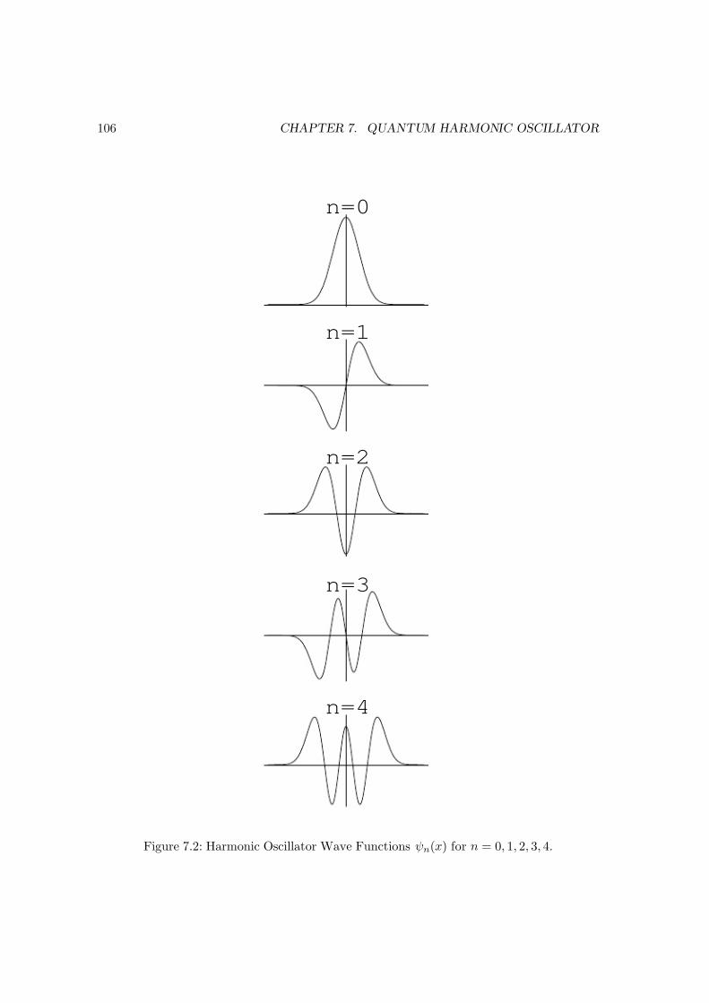
7/27/2019 22BBook.pdf



n=4

n=3

n=2

n=1

n=0

Figure 7.2: Harmonic Oscillator Wave Functions ψn(x) for n = 0, 1, 2, 3, 4.

7/27/2019 22BBook.pdf



7.2.4 Some properties of Hermite polynomials

Solution of Recurrence Relation

To obtain a more explicit formula for the Hermite polynomials we must solve the recurrencerelation (7.13). The polynomials H n(x) are normalized so that the coefficient of the highestpower is 2n. This will determine a0 (when n is even) and a1 (when n is odd). We treat herethe case of n even and leave the case of n odd to the reader. First

an

a0=

a2a0

a4a2

· · · an

an−2

The right hand side of this expression is determined from (7.13) and equals

2(n)

1 · 2

2(n

−2)

3 · 4

2(n

−4)

5 · 6 · · ·2(2)

(n − 1)n

This can be rewritten as2n/2n(n − 2)(n − 4) · · · 4 · 2

n!

This is the ratio an/a0. Requiring that an = 2n gives

a0 = 2n/2 (n − 1)(n − 3)(n − 5) · · · 5 · 3 · 1

We now determine am—the coefficient of xm— (when n is even we can take m even too).Proceeding in a similar manner we write

am

a0= a2

a0a4a2

· · · am

am−2

and again note the right hand side is determined from the recurrence relation ( 7.13); namely,

(−1)m/2 2(n)

1 · 2

2(n − 2)

3 · 4

2(n − 4)

5 · 6· · · 2(n − m + 2)

(m − 1) · m

Multiplying this by the value of a0 we get that am equals

(−1)m/2 2(n+m)/2

m![n(n − 2)(n − 4) · · · (n − m + 2)] [(n − 1)(n − 3) · · · 5 · 3 · 1]

The product of the two quantities in square brackets can be rewritten as

n!

(n − m)!(n − m − 1)(n − m − 3)(n − m − 5) · · · 5 · 3 · 1

Now let m → n − m (so am is the coefficient of xn−m ) to find that am equals

(−1)m/22n−m/2

n

m

1 · 3 · 5 · · · (m − 1)

7/27/2019 22BBook.pdf



where

nm

is the binomial coefficient. Since m is even and runs over 0, 2, 4, . . . n, we can let

m

→2m to get the final formula14

H n(x) = n!

[n/2]m=0

(−1)m

m!(n − 2m)!(2x)n−2m. (7.16)

This same formula holds for n odd if we interpret [n/2] = (n − 1)/2 when n is odd. From(7.16) we can immediately derive the differentiation formula

dH ndx

= 2n H n−1(x). (7.17)

Orthogonality Properties

The harmonic oscillator Hamiltonian H is self-adjoint with distinct eigenvalues. Just as weproved for matrices, it follows that that eigenfunctions ψn are orthogonal. The normalizationconstant N n is chosen so that they are orthonormal. That is if ψn are defined by (7.14),then

(ψn, ψm) = N 2n

∞−∞

H n(x) H m(x) e−x2 dx = δ m,n (7.18)

where N n are defined in (7.15) and δ m,n is the Kronecker delta function.15 The functionsψn are called the harmonic oscillator wave functions .

From the orthogonality relations we can derive what is called the three-term recursion

relation ; namely, we claim that

H n+1(x) − 2xH n(x) + 2nH n−1(x) = 0. (7.19)

Since the highest power of H n has coefficient 2n, we see that

H n+1(x) − 2xH n(x)

must be a polynomial of degree less than or equal to n. Using (7.16) we can see that thehighest power is the same as the highest power of 2n H n−1(x). Thus the left hand side of (7.19) is a polynomial of degree less than or equal to n − 2. It can be written as the linearcombination

c0 H 0(x) + c1 H 1(x) + · · · + cn−2 H n−2(x).

We now multiply both sides of this resulting equation by H k(x) e−x2 , 0 ≤ k ≤ n − 2, andintegrate over all of R. Using the orthogonality relation one concludes that ck = 0.16

14We used the fact that

(2m − 1)!!/(2m)! = 1/(2m m!)

where (2m − 1)!! = (2m − 1)(2m − 3) · · · 5 · 3 · 1.15δm,n equals 1 if m = n and 0 otherwise.16Perhaps the only point that needs clarification is whyZ

R

2xH n(x)H k(x)e−x2

dx

is zero for 0 ≤ k ≤ n − 2. Since 2xH k(x) is a polynomial of degree k + 1 ≤ n − 1, it too can be expandedin terms of Hermite polynomials of degree less than or equal to n − 1; but these are all orthogonal to H n.Hence the expansion coefficients must be zero.

7/27/2019 22BBook.pdf


7.3. SOME PROPERTIES OF THE HARMONIC OSCILLATOR 109

For applications to the harmonic oscillator, it is convenient to find what (7.16) and (7.19)imply for the oscillator wave functions ψn. It is an exercise to show that17

x ψn(x) =

n

2ψn−1(x) +

n + 1

2ψn+1(x) , (7.20)

dψn(x)

dx=

n

2ψn−1(x) −

n + 1

2ψn+1(x) . (7.21)

7.2.5 Completeness of the harmonic oscillator wave functions ψnn≥0

In finite-dimensional vector spaces, we understand the notion of a basis. In particular,we’ve seen the importance of an orthonormal basis. In Hilbert spaces these concepts aremore subtle and a full treatment will not be given here. Here is what can be proved. Forany vector Ψ

∈L2(R) we can find coefficients an such that

Ψ =∞

n=0

anψn. (7.22)

Since this is an infinite sum we must say in what sense this sum converges. If we define thepartial sums

Ψn =n

k=0

akψk,

then we say Ψn → Ψ as n → ∞ if

limn→∞

Ψ − Ψn = 0.

(Observe that Ψn, being a sum of a finite number of terms is well-defined.) Recall that thenorm · in L2(R) is

Ψ − Ψn 2=

R

|Ψ(x) − Ψn(x)|2 dx.

It is in this sense the series converges. Since ψn form an orthonormal sequence, the coeffi-cients an are given simply by

an = (ψn, Ψ) .

Observe that since ψn form an orthonormal basis, the vector Ψ in (7.22) satisfies

Ψ 2=∞

n=0

|an|2 < ∞.

7.3 Some properties of the harmonic oscillator

In quantum mechanics if O is an observable (mathematically, a self-adjoint operator on theHilbert space H), then the average (or expected) value of O in the state Ψ is

O = (OΨ, Ψ) .

17These formulas are valid for n = 0 if we define ψ−1(x) = 0.

7/27/2019 22BBook.pdf



For the quantum oscillator, the average position in the eigenstate ψn is

x = (xψn, ψn) = R

xψn(x)2 dx = 0.

(The integral is zero since ψ2n is an even function of x so that xψn(x)2 is an odd function.)

The average of the square of the position in the eigenstate ψn isx2

=

x2ψn, ψn

.

This inner product (integral) can be evaluated by first using ( 7.20) twice to write x2ψn asa linear combination of the ψk’s:

x2ψn = x

n

2ψn−1 +

n + 1

2ψn+1

=

n2

n − 12ψn−2 +

n2

ψn

+

n + 12

n + 12ψn +

n + 12

ψn+2

=1

2

n(n − 1) ψn−2 + (n +

1

2) ψn +

1

2

n + 1)(n + 2) ψn+2.

The inner product can now be calculated using the orthonormality of the wave functions tofind18

x2

= n +1

2.

A very similar calculation with ˆ p = −i ddx (but this time using (7.21)) gives19

ˆ p = 0,

ˆ p

2= (n +

1

2 ) .

If we define

∆x =

x2 − x2 ,

∆ p =

ˆ p2 − ˆ p2 ,

then (in physical units) we have in state ψn

∆x ∆ p =

n +

1

2

≥

2.

This is the Heisenberg Uncertainty Principle for the harmonic oscillator. The inequality

part of the statement can be shown to be valid under very general conditions.18This is the dimensionless result. Putting back in the dimensions, the average is

(n + 1/2)

mω0

.19Again these are the dimensionless results. Putting back the units the second average is

˙ˆ p2¸

= (n +1

2) mω0.

7/27/2019 22BBook.pdf


7.3. SOME PROPERTIES OF THE HARMONIC OSCILLATOR 111

7.3.1 Averages x(t) and ˆ p(t)

Let Ψ be any state of the system

Ψ(x) =∞

n=0

anψn(x)

such that

A :=n≥0

n

2anan−1, B :=

n≥0

n + 1

2anan+1

are convergent sums. (Here, as throughout, the ψn are the harmonic oscillator wave func-tions.) The time evolution of Ψ is then given by

Ψ(x, t) = n≥0

ane−iE nt/ ψn(x) (7.23)

which follows from the above discussion of separation of variables.

In the state Ψ(x, t) we are interested in computing the average values of x and ˆ p. Fornotationally convenience let’s define

xavg(t) = x = (xΨ(x, t), Ψ(x, t))

and pavg(t) = ˆ p = (ˆ pΨ(x, t), Ψ(x, t)) .

Letx0 := xavg(0) = (xΨ(x, 0), Ψ(x, 0))

and p0 := pavg(0) = (ˆ pΨ(x, 0), Ψ(x, 0)) .

We first calculate x0 and p0.

x0 =

m,n≥0

anam (xψn, ψm)

=

m,n≥0

anam

n

2(ψn−1, ψm) +

n + 1

2(ψn+1, ψm)

=

m,n≥0

anam

n

2δ n−1,m +

n + 1

2δ n+1,m

= A + Bwhere we use the orthonormality of the functions ψn. Similarly,

p0 = −iA + iB.

We now calculate xavg(t) Now the state is (7.23). Proceeding as in the t = 0 case we see

xavg(t) =

m,n≥0

aname−i(E n−E m)t/ (xψn, ψm) .

7/27/2019 22BBook.pdf



The calculation of the inner products (xψn, ψm) was done in the t = 0 case. Noting that

E n − E n−1 = ω0 and E n − E n+1 = − ω0,

we see thatxavg(t) = e−iω0t A + eiω0t B. (7.24)

Similarly, we find pavg(t) = −ie−iω0t A + ieiω0t B. (7.25)

Writing these averages in terms of sines and cosines and using the above expressions for x0and p0, we see that the average position and momentum in the state Ψ( x, t) evolve accordingto20

xavg(t) = x0 cos(ω0t) +p0

mω0sin(ω0t) (7.26)

pavg(t) = p0

cos(ω0

t)−

mω0

x0

sin(ω0

t) (7.27)

One should now compare the time evolution of the quantum averages (7.26) and (7.27)with the time evolution of the classical position and momentum (7.1) and (7.2). They areidentical. It is a special property of the quantum harmonic oscillator that the quantumaverages exactly follow the classical trajectories. More generally, one expects this to occuronly for states whose wave function remains localized in a region of space.

20We restore the physical units in these last equations

7/27/2019 22BBook.pdf


7.4. THE HEISENBERG UNCERTAINTY PRINCIPLE 113

7.4 The Heisenberg Uncertainty Principle

The more precisely the position is determined, the less precisely the momentumis known in this instant, and vice versa. Werner Heisenberg, 1927.

In §7.3 we proved the Heisenberg Uncertainty Principle for the special case of the harmonicoscillator. Here we show this is a general feature of quantum mechanics. First we recallsome basic facts about complex vector spaces.

1. If Ψ and Φ are any two states in our Hilbert space of states H, we have an innerproduct defined (Ψ, Φ) that satisfies the properties

(a) (Ψ, Φ) = (Φ, Ψ) where z denotes the complex conjugate of z.

(b) (c1Ψ1 + c2Ψ2, Φ) = c1 (Ψ1, Φ) + c2 (Ψ2, Φ) for all states Ψ1, Ψ2 and all complex

numbers c1, c2.(c) The length or norm of the state Ψ is defined to be Ψ2 = (Ψ, Ψ) ≥ 0 with

Ψ = 0 if and only if Ψ = 0, the zero vector in H.

2. An operator A is called Hermitian (or self-adjoint) if

(AΨ, Φ) = (Ψ, AΦ)

for all states Ψ, Φ. In quantum mechanics observables are assumed to be Hermitian.Note this makes the expected value of the observable A in state Ψ a real number

A := (AΨ, Ψ)

= (Ψ, AΨ)

= (AΨ, Ψ)

= A.

Sometimes one writes AΨ to denote the state in which the expected value is com-puted.

3. Just as in linear algebra, we have the Cauchy-Schwarz inequality

|(Ψ, Φ)|2 ≤ Ψ2 Φ2 (7.28)

for all states Ψ, Φ ∈ H.

We now assume we have observables A and B that satisfy the commutation relation

AB

−BA = i id (7.29)

where id is the identity operator and i is the imaginary number, i2 = −1. We showed earlierthat in units where = 1 the position and momentum operators satisfy such a commutationrelation. For a given state Ψ and observable A we define21

∆A =

(A − A)

2

=

A2 − A2 ≥ 0.

21In classical probability ∆A is called the standard deviation of A. The quantity ∆A is a measure of thedeviation of A from its expected value A.



7/27/2019 22BBook.pdf



We now prove that if observables A and B satisfy (7.29) then

∆A · ∆B ≥1

2 . (7.30)

Proof: Let Ψ denote any normalized state vector, i.e. Ψ = 1. Apply (7.29) to Ψ to obtain

ABΨ − BAΨ = iΨ

Now take the inner product of each side with the state Ψ to obtain

(ABΨ, Ψ) − (BAΨ, Ψ) = i (Ψ, Ψ)

which simplifies to22

(BΨ, AΨ) − (AΨ, BΨ) = i (7.31)

Let t denote any real number, then by the Cauchy-Schwarz inequality (7.28)

|(Ψ, AΨ + itBΨ)|2 ≤ AΨ + itBΨ2 (7.32)

since Ψ = 1. Let’s simplify the left-hand side of (7.32)(Ψ, AΨ + itBΨ) = (Ψ, AΨ) − it(Ψ, BΨ) = A − itB.

The absolute value squared of this is

A2 + t2B2.

We now examine the right-hand side of (7.32)

AΨ + itBΨ2 = (AΨ + itBΨ, AΨ + itBΨ)

= AΨ2 + it (BΨ, AΨ) − (AΨ, BΨ) + t2BΨ2= AΨ2 − t + t2BΨ2 by use of (7.31). (7.33)

Thus the inequality (7.32) becomes

A2

+ t

2

B2

≤ AΨ2

− t + t

2

BΨ2

.Using the fact that AΨ2 = (AΨ, AΨ) = (A2Ψ, Ψ) = A2 (and similarly for B) and thedefinition of ∆A (and similarly for ∆B), the above inequality can be rewritten as

t2 (∆B)2 − t + (∆A)

2 ≥ 0.

This holds for all real t. The above is a quadratic polynomial in t that is always nonnegative.This means that the discriminant of the quadratic polynomial must be nonpositive, i.e.b2 − 4ac ≤ 0. That is,

1 − 4 (∆A)2

(∆B)2 ≤ 0

which implies that

∆A · ∆B ≥ 1

2which is what we want to prove.

When A is the position operator and B is the momentum operator we get the HeisenbergUncertainty Principle which states

∆x · ∆ p ≥

2where we have returned to physical units. The appearance of Planck’s constant in theright hand side shows that sets the scale for quantum mechanical phenomena.

22Note (ABΨ, Ψ) = (BΨ, AΨ) and (BAΨ, Ψ) = (AΨ, BΨ) since A and B are Hermitian. Also note onthe right hand side we used the fact that (Ψ, Ψ) = Ψ2 = 1.

7/27/2019 22BBook.pdf


7.5. EXERCISES 115

7.5 Exercises

#1.

Using (7.17) and (7.19), prove (7.20) and (7.21).

#2. Averages x4 and ˆ p4:

For the state ψn, compute the averages x4 and ˆ p4.

#3.

Prove (7.25). (The proof is similar to the proof of (7.24).)

#4.

Define the operators

a =1√

2

x +

d

dx

a∗ =1√

2

x − d

dx

That is, if ψ = ψ(x), then

(aψ)(x) =1√

2

xψ(x) +

dψ

dx

and similarly for a∗. Using (7.20) and (7.21) show that for the harmonic oscillator wavefunctions ψn

aψn =√

n ψn−1, n ≥ 1, aψ0 = 0,

a∗ψn =√

n + 1 ψn+1, n = 0, 1, . . . ,

a∗aψn = n ψn, n = 0, 1, . . . ,

(aa∗

− a∗

a) ψn = ψn, n = 0, 1, . . . .

Explain why this last equation implies the operator equation

[a, a∗] = id.

In quantum mechanics the operator a is called an annihilation operator and the operatora∗ is called a creation operator . On the basis of this exercise, why do you think they havethese names?

7/27/2019 22BBook.pdf



#5. Hermite Polynomials

We obtained the Hermite polynomials from the recurrence relation (7.13). Alternatively,we have a generating formula for the Hermite polynomials. Starting with this (which manybooks take as the definition of the Hermite polynomials), we may obtain the Schr odingerequation.

1. Verify that the first three Hermite polynomials H 0(ξ ), H 1(ξ ) and H 2(ξ ) are given usingthe generating formula

H n(ξ ) = (−1)neξ2

dn

dξ ne−ξ2

(7.34)

2. The generating function (7.34) can be used to give an alternative generating functionfor Hermite polynomials. Show that

e−z2+2zξ =∞

n=0

zn

n!H n(ξ ) . (7.35)

Hint: Let F (z) = e−z2 and consider the Taylor expansion of eξ2F (z − ξ ) about thepoint z = 0.

3. Derive (7.17) from (7.35). Now derive (7.19) using (7.34) and the newly derived (7.17).

4. Use (7.17) and (7.19) to show that the Hermite polynomials are solutions of the Her-

mite equation d2

dξ 2H n(ξ ) − 2ξ

d

dξ H n(ξ ) + 2nH n(ξ ) = 0. (7.36)

5. We know that the Hermite polynomials satisfy

N 2n

∞−∞

H n(ξ )H m(ξ )e−ξ2dξ = δ nm. (7.37)

Here by setting ψn(ξ ) = N nH n(ξ )e−ξ2/2 we see that ψn(ξ ) are orthonormal in L2(R).Use (7.36) to obtain the differential equation that ψn(ξ ) satisfy. You should obtain

(7.9) with ε = 2n + 1. This implies that ψn(ξ ) = N nH n(ξ )e−ξ2/2 is the eigenfunctioncorresponding to the eigenvalue of the Hamiltonian operator.

7/27/2019 22BBook.pdf


Chapter 8

Laplace Transform

8.1 Matrix version of the method of Laplace transforms

for solving constant coefficient DE’s

The Laplace transform of a function f (t) is

F (s) = L(f )(s) =

∞0

e−tsf (t) dt (8.1)

for s sufficiently large. For the Laplace transform to make sense the function f cannot growfaster that an exponential near infinity. Thus, for example, the Laplace transform of ex2 isnot defined.

We extend (8.1) to vector-valued functions f (t),

f (t) =

f 1(t)f 2(t)

...f n(t)

(8.2)

by

F (s) = L(f )(s) =

∞0

e−tsf 1(t) dt ∞0

e−tsf 2(t) dt...

∞0

e−tsf n

(t) dt

. (8.3)

Integration by parts shows that

L(df

dt)(s) = sL(f )(s) − f (0). (8.4)

We now explain how matrix Laplace transforms are used to solve the matrix ODE

dx

dt= Ax + f (t) (8.5)

117

7/27/2019 22BBook.pdf


118 CHAPTER 8. LAPLACE TRANSFORM

where A is a constant coefficient n × n matrix, f (t) is a vector-valued function of theindependent variable t (“forcing term”) with initial condition

x(0) = x0. (8.6)

First, we take the Laplace transform of both sides of (8.5). From (8.4) we see that theLaplace transform of the LHS of (8.5) is

L(dx

dt) = sL(x) − x0.

The Laplace transform of the RHS of (8.5) is

L(Ax + f ) = L(Ax) + L(f )

= A

L(x) + F (s)

where we set F (s) = L(f )(s) and we used the fact that A is independent of t to conclude1

L(Ax) = AL(x). (8.7)

Thus the Laplace transform of (8.5) is

sL(x) − x0 = AL(x) + F,

or

(sI n − A)L(x) = x0 + F (s) (8.8)

where I n is the n

×n identity matrix. Equation (8.8) is a linear system of algebraic equations

for L(x). We now proceed to solve (8.8). This can be done once we know that (sI n − A) isinvertible. Recall that a matrix is invertible if and only if the determinant of the matrix isnonzero. The determinant of the matrix in question is

p(s) := det(sI n − A), (8.9)

which is the characteristic polynomial of the matrix A. We know that the zeros of p(s) arethe eigenvalues of A. If s is larger than the absolute value of the largest eigenvalue of A; insymbols,

s > max|λi|, (8.10)

then p(s) cannot vanish and hence (sI n − A)−1 exists. We assume s satisfies this condition.Then multiplying both sides of (8.8) by (sI n

−A)−1 results in

L(x)(s) = (sI n − A)−1x0 + (sI n − A)−1F (s). (8.11)

1You are asked to prove (8.7) in an exercise.

7/27/2019 22BBook.pdf


8.1. MATRIX VERSION 119

Equation (8.11) is the basic result in the application of Laplace transforms to the solutionof constant coefficient differential equations with an inhomogeneous forcing term. Equation

(8.11) will be a quick way to solve initial value problems once we learn efficient methodsto (i) compute (sI n − A)−1, (ii) compute the Laplace transform of various forcing termsF (s) = L(f )(s), and (iii) find the inverse Laplace transform. Step (i) is easier if oneuses software packages such as MatLab . Steps (ii) and(iii) are made easier by the use of extensive Laplace transform tables or symbolic integration packages such as Mathematica.It should be noted that many of the DE techniques one learns in engineering courses canbe described as efficient methods to do these three steps for examples that are of interest toengineers.

We now give two examples that apply (8.11).

8.1.1 Example 1

Consider the scalar ODEd2y

dt2+ b

dy

dt+ cy = f (t) (8.12)

where b and c are constants. We first rewrite this as a system

x(t) =

x1

x2

=

y(t)y′(t)

so thatdx

dt=

0 1

−c −b

x +

0

f (t)

.

Then

sI 2 − A =s

−1

c s + b

,

and

(sI 2 − A)−1 =1

s2 + bs + c

s + b 1−c s

.

Observe that the characteristic polynomial

p(s) = det(sI 2 − A) = s2 + bs + c

appears in the denominator of the matrix elements of (sI 2 − A)−1. (This factor in Laplacetransforms should be familiar from the scalar treatment—here we see it is the characteristicpolynomial of A.) By (8.11)

L(x)(s) = 1s2 + bs + c

(s + b)y(0) + y

′

(0)−cy(0) + sy′(0)

+ F (s)s2 + bs + c

1s

where F (s) = L(f )(s). This implies that the Laplace transform of y(t) is given by

L(y)(s) =(s + b)y(0) + y′(0)

s2 + bs + c+

F (s)

s2 + bs + c. (8.13)

This derivation of (8.13) may be compared with the derivation of equation (16) on page 302of Boyce and DiPrima [4] (in our example a = 1).

7/27/2019 22BBook.pdf



8.1.2 Example 2

We consider the system (8.5) for the special case of n = 3 with f (t) = 0 and A given by

A =

1 0 −1

1 2 11 −1 −1

. (8.14)

The characteristic polynomial of (8.14) is

p(s) = s3 − 2s2 + s − 2 = (s2 + 1)(s − 2) (8.15)

and so the matrix A has eigenvalues ±i and 2. A rather long linear algebra computationshows that

(sI 3−

A)−1 =1

p(s)

s2 − s − 1 1 −s + 2s + 2 s2 s

−2

s − 3 −s + 1 s2 − 3s + 2 . (8.16)

If one writes a partial fraction decomposition of each of the matrix elements appearing in(8.16) and collects together terms with like denominators, then (8.16) can be written as

(sI 3 − A)−1 =1

s − 2

1/5 1/5 0

4/5 4/5 0−1/5 −1/5 0

+1

s2 + 1

(3 + 4s)/5 −(2 + s)/5 −1

−(3 + 4s)/5 (2 + s)/5 1(7 + s)/5 (−3 + s)/5 −1 + s

. (8.17)

We now apply (8.17) to solve (8.5) with the above A and f = 0 for the case of initial

conditions

x0 =

1

−21

. (8.18)

We find

L(x)(s) = (sI 3 − A)−1x0 =1

s − 2

−1/5

−4/51/5

+

s

s2 + 1

6/5

−6/54/5

+

1

s2 + 1

2/5

−2/58/5

. (8.19)

To find x(t) from (8.19) we use Table 6.2.1 on page 300 of Boyce and DiPrima [4]; inparticular, entries 2, 5, and 6. Thus

x(t) = e2t−

1/5

−4/51/5

+ cos t 6/5

−6/54/5

+ sin t 2/5

−2/58/5

.

One can also use Mathematica to compute the inverse Laplace transforms. To do so usethe command InverseLaplaceTransform. For example if one inputsInverseLaplaceTransform[1/(s-2),s,t] then the output is e2t.

We give now a second derivation of (8.19) using the eigenvectors of A. As noted above,the eigenvalues of A are λ1 = 2, λ2 = i, and λ3 = −i. If we denote by φj an eigenvector

7/27/2019 22BBook.pdf


8.2. STRUCTURE OF (SI N − A)−1 121

associated to eigenvalue λj ( j = 1, 2, 3), then a routine linear algebra computation gives thefollowing possible choices for the φj :

φ1 =

−1

−41

, φ2 =

(1 + i)/2

−(1 + i)/21

, φ3 =

(1 − i)/2

(−1 + i)/21

.

Now for any eigenvector φ corresponding to eigenvalue λ of a matrix A we have

(sI n − A)−1φ = (s − λ)−1φ.

To use this observation we first write

x0 = c1φ1 + c2φ2 + c3φ3.

A computation shows that

c1 = 1/5, c2 = 2/5 − 4i/5, and c3 = 2/5 + 4i/5.

Thus

(sI 3 − A)−1x0 =1

5(s − 2)−1φ1 +

2 − 4i

5(s − i)−1φ2 +

2 + 4i

5(s + i)−1φ3.

Combining the last two terms gives (8.19).

8.2 Structure of (sI n − A)−1 when A is diagonalizable

In this section we assume that the matrix A is diagonalizable; that is, we assume a set of linearly independent eigenvectors of A form a basis. Recall the following two theorems fromlinear algebra: (1) If the n×n matrix A has n distinct eigenvalues, then A is diagonalizable;and (2) If the matrix A is symmetric (hermitian if the entries are complex), then A isdiagonalizable.

Since A is assumed to be diagonalizable, there exists a nonsingular matrix P such that

A = P DP −1

where D is

D =

λ1 0 . . . 00 λ2 . . . 0

......

. . . ...0 0 . . . λn

and each eigenvalue λi of A appears as many times as the (algebraic) multiplicity of λi.Thus

sI n − A = sI n − P DP −1

= P (sI n − D)P −1 ,

7/27/2019 22BBook.pdf



so that

(sI n − A)

−1

=

P (sI n − D)P

−1

)−1

= P (sI n − D)−1P −1.

Since P and P −1 are independent of s, the s dependence of (sI n − A)−1 resides in thediagonal matrix (sI n − D)−1. This tells us that the partial fraction decomposition of thematrix (sI n − A)−1 is of the form

(sI n − A)−1 =n

j=1

1

s − λjP j

whereP j = P E jP −1

and E j is the diagonal matrix with all zeros on the main diagonal except for 1 at the ( j, j)thentry. This follows from the fact that

(sI n − D)−1 =

nj=1

1

s − λjE j

Note that P j have the property thatP 2j = P j .

Such matrices are called projection operators .

In general, it follows from Cramer’s method of computing the inverse of a matrix, that thegeneral structure of (sI n −A)−1 will be 1/p(s) times a matrix whose entries are polynomialsof at most degree n − 1 in s. When an eigenvalue, say λ1, is degenerate and of (algebraic)multiplicity m1, then the characteristic polynomial will have a factor (s − λ1)m1 . We haveseen that if the matrix is diagonalizable, upon a partial fraction decomposition only a single

power of (s − λ1) will appear in the denominator of the partial fraction decompostion.Finally, we conclude by mentioning that when the matrix A is not diagonalizable, then thisis reflected in the partial fraction decomposition of (sI n − A)−1 in that some powers of (s − λj) occur to a higher degree than 1.

8.3 Exercises

#1.

Use the Laplace transform to find the solution of the initial value problem

dx

dt=

1 −1 00

−1 1

0 1 −1 x +

0120 , x(0) =

000 .

#2.

Let A be a n × n matrix whose entries are real numbers and x ∈ Rn. Prove that

L(Ax) = AL(x)

where L denotes the Laplace transform.

7/27/2019 22BBook.pdf


8.3. EXERCISES 123

#3.

Let E j denote the diagonal n × n matrix with all zeros on the main diagonal except for 1at the ( j, j) entry.

• Prove that E 2j = E j .

• Show that if P is any invertible n × n matrix, then P 2j = P j where P j := P E jP −1.

#4.

It is a fact that you will learn in an advanced linear algebra course, that if a 2 × 2 matrixA is not diagonalizable, then there exists a nonsingular matrix P such that

A = P B P −1

where

B =

λ 10 λ

for some constant λ.

• Show that λ must be an eigenvalue of A with algebraic multiplicity 2.

• Find an eigenvector of A (in terms of the matrix P ), and show that A has no othereigenvectors (except, of course, scalar multiples of the vector you have already found).

• Show that

(sI 2 − A)−1 =1

s − λP E 1P −1 +

1

s − λP E 2P −1 +

1

(s − λ)2P N P −1

where

N =

0 10 0

.

• Relate what is said here to the remarks in the footnote in Exercise 5.5.2.

7/27/2019 22BBook.pdf



7/27/2019 22BBook.pdf


Bibliography

[1] V. I. Arnold, Mathematical Methods of Classical Mechanics , 2nd ed., Springer-Verlag, N.Y. 1989.

[2] V. I. Arnold, Ordinary Differential Equations , Second printing of the 1992 edition,Springer-Verlag, Berlin, 2006.

[3] G. Birkhoff and G-C Rota, Ordinary Differential Equations 4th ed., John Wiley &Sons, 1989.

[4] W. E. Boyce and R. C. DiPrima, Elementary Differential Equations and Boundary

Value Problems , 7th–9th eds., John Wiley & Sons.

[5] G. Chen, P. J. Morris and J. Zhou, Visualization of special eigenmode shapes of avibrating elliptical membrane, SIAM Review 36 (1994), 453–469.

[6] B. Temple and C. A. Tracy, From Newton to Einstein, American Math. Monthly99 (1992), 507–512.

125

7/27/2019 22BBook.pdf


Index

Acceleration due to gravity, 2Acoustic phonons, 96Angular momentum, 28Annihilation and creation operators, 115Arnold, Vladimir, 57

Bessel functions, 88Binet’s equation, 30

Catalan numbers, 55Classical harmonic oscillator, 20, 37

Forced oscillations, 43Friction, 27

Commutator, 101Complex exponential function, 40

Addition formula, 40Euler’s formula, 40

Difference equations, 52

Constant coefficients, 52Catalan numbers, 55Fibonnaci numbers, 53

Differential equation, definition, 11Dirac, Paul, 99

Energy conservation, 16, 20Euler’s equation, 48Euler’s formula, 33Euler, Leonhard, 33

Fibonacci, Leonardo, 51Fibonnaci numbers, 53

Half-life, 25Harmonic oscillator, 20, 37, 64, 84

Forced oscillations, 43Quantum, 101

Harmonic oscillator wave functions, 108Heisenberg Uncertainty Principle, 113Heisenberg Uncertainty Relation, 102Helmholtz equation, 85, 95

Hermite polynomials, 103, 105, 107, 108, 115Generating functions, 115

Hooke’s Law, 17Forced oscillations, 43

Resonance, 45Frequency, 20

Friction, 27Nonlinear correction, 27

Hooke, Robert, 1

Integrating factor, 12

Kinetic energy, 16, 97, 102Kolmogorov forward equations, 67

Laplace transform, 117Application to radioactive decay, 66

Laplacian, 86Lax pairs, 93

Linear first order ODE, 11integrating factor, 12Loan payments, 13

MatLab, 5, 23, 42Symbolic Math Toolbox, 5

Matrix exponential, 58Applied to matrix ODE, 60Nilpotent matrix, 65

Matrix ODE, 60Alternating masses-spring problem, 96Inhomogeneous, 63Radioactive decay, 66

Newton’s equations, 2, 16, 70, 91, 100Central field, 28Inverse square law, 29

Newton’s principle of determinacy, 1Normal modes, 74

Optical phonons, 96Order of a DE, 11

126

7/27/2019 22BBook.pdf


INDEX 127

Pendulum, 2Coupled, 90

Period, 20Planck’s constant, 100Population dynamics, 26Potential energy, 16, 97, 102

Quantum harmonic oscillator, 101Annihilation and creation operators, 115Hermite polynomials, 105Quantization of energy, 105

Quantum mechanics, 100State space, 100

Reduction of order, 37

Rigid body motion, 30

Schrodinger equation, 100Schrodinger, Erwin, 99Second order linear ODE, 34

Bessel functions, 88Constant coefficients, 38Vector space of solutions, 34Wronskian, 35

Toda chain, 93

Vibrating membrane, 85

Circular domain, 87Elliptical domain 89

Documents

22BBook.pdf