Embed Size (px)
Citation preview
Classical MechanicsNumerical ExampleDiscrete Mechanics
Taylor Variational IntegratorDiscrete Hamiltonian Variational Integrators
Advancement Talk
Jeremy Schmitt
June 17, 2015
Jeremy Schmitt Advancement Talk
Classical MechanicsNumerical ExampleDiscrete Mechanics
Taylor Variational IntegratorDiscrete Hamiltonian Variational Integrators
Outline
1 Classical Mechanics
2 Numerical Example
3 Discrete Mechanics
4 Taylor Variational Integrator
5 Discrete Hamiltonian Variational Integrators
Jeremy Schmitt Advancement Talk
Classical MechanicsNumerical ExampleDiscrete Mechanics
Taylor Variational IntegratorDiscrete Hamiltonian Variational Integrators
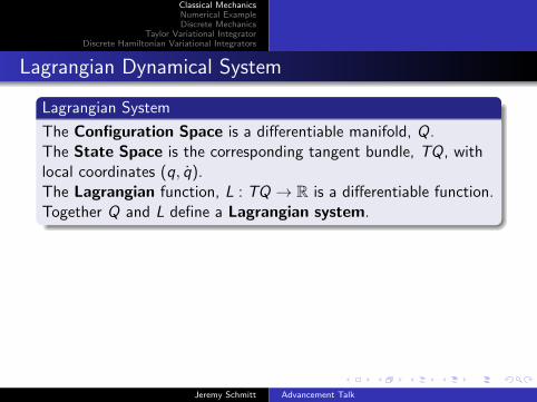
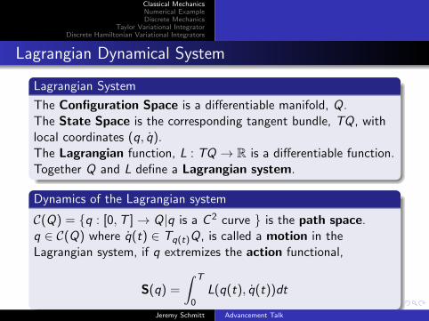
Lagrangian Dynamical System
Lagrangian System
The Configuration Space is a differentiable manifold, Q.The State Space is the corresponding tangent bundle, TQ, withlocal coordinates (q, q).The Lagrangian function, L : TQ → R is a differentiable function.Together Q and L define a Lagrangian system.
Dynamics of the Lagrangian system
C(Q) = {q : [0,T ]→ Q|q is a C 2 curve } is the path space.q ∈ C(Q) where q(t) ∈ Tq(t)Q, is called a motion in theLagrangian system, if q extremizes the action functional,
S(q) =
∫ T
0L(q(t), q(t))dt
Jeremy Schmitt Advancement Talk
Classical MechanicsNumerical ExampleDiscrete Mechanics
Taylor Variational IntegratorDiscrete Hamiltonian Variational Integrators
Lagrangian Dynamical System
Lagrangian System
The Configuration Space is a differentiable manifold, Q.The State Space is the corresponding tangent bundle, TQ, withlocal coordinates (q, q).The Lagrangian function, L : TQ → R is a differentiable function.Together Q and L define a Lagrangian system.
Dynamics of the Lagrangian system
C(Q) = {q : [0,T ]→ Q|q is a C 2 curve } is the path space.q ∈ C(Q) where q(t) ∈ Tq(t)Q, is called a motion in theLagrangian system, if q extremizes the action functional,
S(q) =
∫ T
0L(q(t), q(t))dt
Jeremy Schmitt Advancement Talk

Classical MechanicsNumerical ExampleDiscrete Mechanics
Taylor Variational IntegratorDiscrete Hamiltonian Variational Integrators
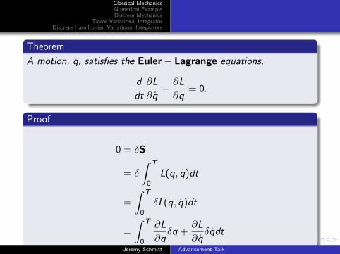
Theorem
A motion, q, satisfies the Euler − Lagrange equations,
d
dt
∂L
∂q− ∂L
∂q= 0.
Proof
0 = δS
= δ
∫ T
0L(q, q)dt
=
∫ T
0δL(q, q)dt
=
∫ T
0
∂L
∂qδq +
∂L
∂qδqdt
Jeremy Schmitt Advancement Talk
Classical MechanicsNumerical ExampleDiscrete Mechanics
Taylor Variational IntegratorDiscrete Hamiltonian Variational Integrators
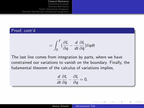
Proof, cont’d
=
∫ T
0(∂L
∂q− d
dt
∂L
∂q)δqdt
The last line comes from integration by parts, where we haveconstrained our variations to vanish on the boundary. Finally, thefudamental theorem of the calculus of variations implies,
d
dt
∂L
∂q− ∂L
∂q= 0.
Jeremy Schmitt Advancement Talk
Classical MechanicsNumerical ExampleDiscrete Mechanics
Taylor Variational IntegratorDiscrete Hamiltonian Variational Integrators
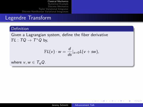
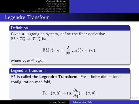
Legendre Transform
Definition
Given a Lagrangian system, define the fiber derivativeFL : TQ → T ∗Q by,
FL(v) · w =d
ds|s=0L(v + sw),
where v ,w ∈ TqQ.
Legendre Transform
FL is called the Legendre Transform. For a finite dimensionalconfiguration manifold,
FL : (q, q)→ (q,∂L
∂q) = (q, p).
Jeremy Schmitt Advancement Talk
Classical MechanicsNumerical ExampleDiscrete Mechanics
Taylor Variational IntegratorDiscrete Hamiltonian Variational Integrators
Legendre Transform
Definition
Given a Lagrangian system, define the fiber derivativeFL : TQ → T ∗Q by,
FL(v) · w =d
ds|s=0L(v + sw),
where v ,w ∈ TqQ.
Legendre Transform
FL is called the Legendre Transform. For a finite dimensionalconfiguration manifold,
FL : (q, q)→ (q,∂L
∂q) = (q, p).
Jeremy Schmitt Advancement Talk
Classical MechanicsNumerical ExampleDiscrete Mechanics
Taylor Variational IntegratorDiscrete Hamiltonian Variational Integrators
Definition
The generalized momentum coordinates, p ∈ T ∗Q, are defined by,
p =∂L
∂q
Hamiltonian
Assuming FL is a diffeomorphism, define the HamiltonianH : T ∗Q → R as,
H(q, p) = pq − L(q, q)|p= ∂L∂q.
Jeremy Schmitt Advancement Talk

Classical MechanicsNumerical ExampleDiscrete Mechanics
Taylor Variational IntegratorDiscrete Hamiltonian Variational Integrators
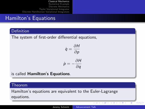
Hamilton’s Equations
Definition
The system of first-order differential equations,
q =∂H
∂p
p = −∂H
∂q
is called Hamilton′s Equations.
Theorem
Hamilton’s equations are equivalent to the Euler-Lagrangeequations.
Jeremy Schmitt Advancement Talk
Classical MechanicsNumerical ExampleDiscrete Mechanics
Taylor Variational IntegratorDiscrete Hamiltonian Variational Integrators
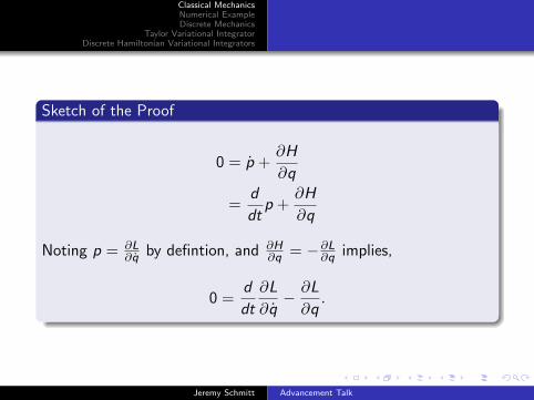
Sketch of the Proof
0 = p +∂H
∂q
=d
dtp +
∂H
∂q
Noting p = ∂L∂q by defintion, and ∂H
∂q = −∂L∂q implies,
0 =d
dt
∂L
∂q− ∂L
∂q.
Jeremy Schmitt Advancement Talk
Classical MechanicsNumerical ExampleDiscrete Mechanics
Taylor Variational IntegratorDiscrete Hamiltonian Variational Integrators
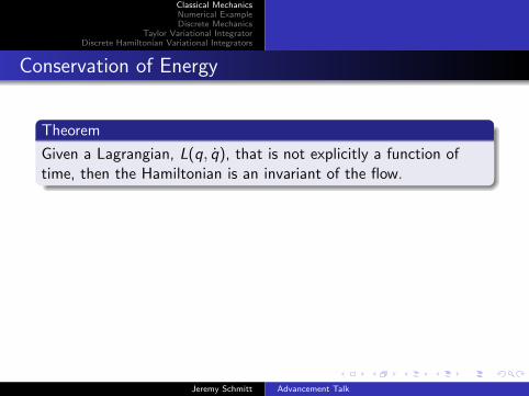
Conservation of Energy
Theorem
Given a Lagrangian, L(q, q), that is not explicitly a function oftime, then the Hamiltonian is an invariant of the flow.
Proof
dH
dt=∂H
∂q
dq
dt+∂H
∂p
dp
dt
= −pq + qp
= 0
Jeremy Schmitt Advancement Talk
Classical MechanicsNumerical ExampleDiscrete Mechanics
Taylor Variational IntegratorDiscrete Hamiltonian Variational Integrators
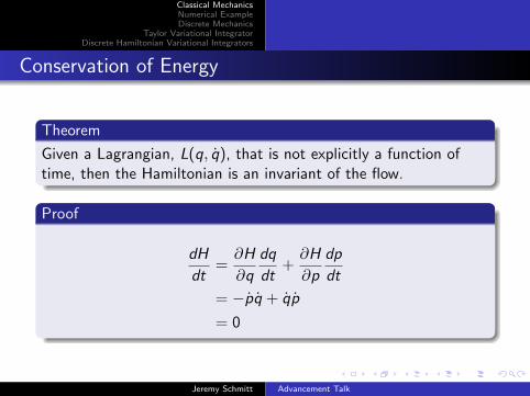
Conservation of Energy
Theorem
Given a Lagrangian, L(q, q), that is not explicitly a function oftime, then the Hamiltonian is an invariant of the flow.
Proof
dH
dt=∂H
∂q
dq
dt+∂H
∂p
dp
dt
= −pq + qp
= 0
Jeremy Schmitt Advancement Talk
Classical MechanicsNumerical ExampleDiscrete Mechanics
Taylor Variational IntegratorDiscrete Hamiltonian Variational Integrators
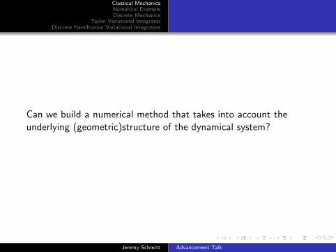
Can we build a numerical method that takes into account theunderlying (geometric)structure of the dynamical system?
Jeremy Schmitt Advancement Talk
Classical MechanicsNumerical ExampleDiscrete Mechanics
Taylor Variational IntegratorDiscrete Hamiltonian Variational Integrators
Outline
1 Classical Mechanics
2 Numerical Example
3 Discrete Mechanics
4 Taylor Variational Integrator
5 Discrete Hamiltonian Variational Integrators
Jeremy Schmitt Advancement Talk
Classical MechanicsNumerical ExampleDiscrete Mechanics
Taylor Variational IntegratorDiscrete Hamiltonian Variational Integrators
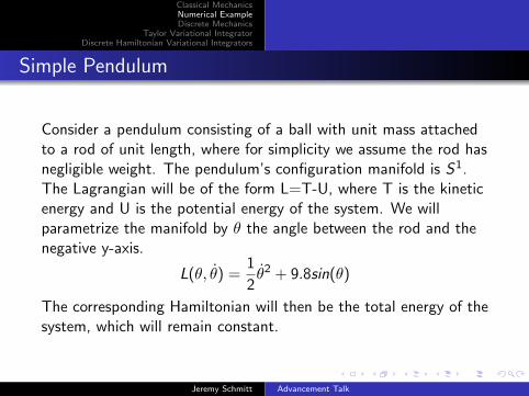
Simple Pendulum
Consider a pendulum consisting of a ball with unit mass attachedto a rod of unit length, where for simplicity we assume the rod hasnegligible weight. The pendulum’s configuration manifold is S1.The Lagrangian will be of the form L=T-U, where T is the kineticenergy and U is the potential energy of the system. We willparametrize the manifold by θ the angle between the rod and thenegative y-axis.
L(θ, θ) =1
2θ2 + 9.8sin(θ)
The corresponding Hamiltonian will then be the total energy of thesystem, which will remain constant.
Jeremy Schmitt Advancement Talk
Classical MechanicsNumerical ExampleDiscrete Mechanics
Taylor Variational IntegratorDiscrete Hamiltonian Variational Integrators
Simple Pendulum
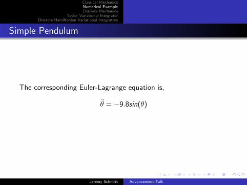
The corresponding Euler-Lagrange equation is,
θ = −9.8sin(θ)
Jeremy Schmitt Advancement Talk
Classical MechanicsNumerical ExampleDiscrete Mechanics
Taylor Variational IntegratorDiscrete Hamiltonian Variational Integrators
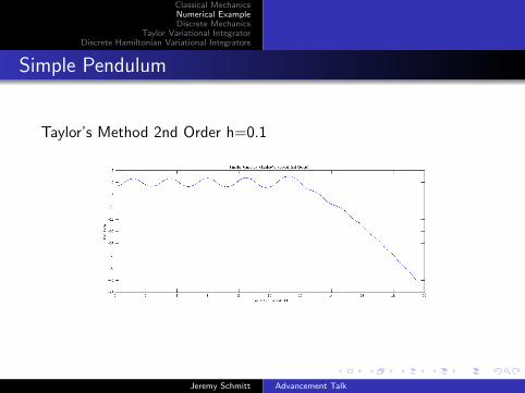
Simple Pendulum
Taylor’s Method 2nd Order h=0.1
Jeremy Schmitt Advancement Talk

Classical MechanicsNumerical ExampleDiscrete Mechanics
Taylor Variational IntegratorDiscrete Hamiltonian Variational Integrators
Simple Pendulum
Taylor Variational Integrator 2nd Order(TVI2) h=0.1
Jeremy Schmitt Advancement Talk
Classical MechanicsNumerical ExampleDiscrete Mechanics
Taylor Variational IntegratorDiscrete Hamiltonian Variational Integrators
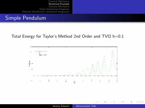
Simple Pendulum
Total Energy for Taylor’s Method 2nd Order and TVI2 h=0.1
Jeremy Schmitt Advancement Talk
Classical MechanicsNumerical ExampleDiscrete Mechanics
Taylor Variational IntegratorDiscrete Hamiltonian Variational Integrators
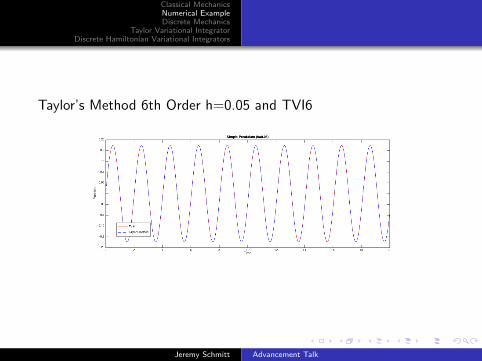
Taylor’s Method 6th Order h=0.05 and TVI6
Jeremy Schmitt Advancement Talk
Classical MechanicsNumerical ExampleDiscrete Mechanics
Taylor Variational IntegratorDiscrete Hamiltonian Variational Integrators
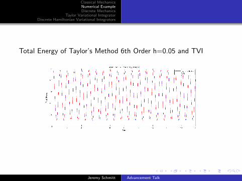
Total Energy of Taylor’s Method 6th Order h=0.05 and TVI
Jeremy Schmitt Advancement Talk
Classical MechanicsNumerical ExampleDiscrete Mechanics
Taylor Variational IntegratorDiscrete Hamiltonian Variational Integrators
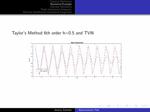
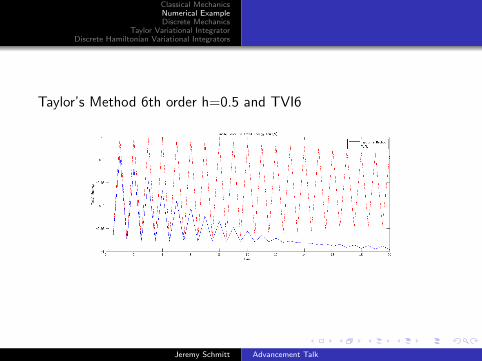
Taylor’s Method 6th order h=0.5 and TVI6
Jeremy Schmitt Advancement Talk
Classical MechanicsNumerical ExampleDiscrete Mechanics
Taylor Variational IntegratorDiscrete Hamiltonian Variational Integrators
Taylor’s Method 6th order h=0.5 and TVI6
Jeremy Schmitt Advancement Talk

Classical MechanicsNumerical ExampleDiscrete Mechanics
Taylor Variational IntegratorDiscrete Hamiltonian Variational Integrators
Outline
1 Classical Mechanics
2 Numerical Example
3 Discrete Mechanics
4 Taylor Variational Integrator
5 Discrete Hamiltonian Variational Integrators
Jeremy Schmitt Advancement Talk
Classical MechanicsNumerical ExampleDiscrete Mechanics
Taylor Variational IntegratorDiscrete Hamiltonian Variational Integrators
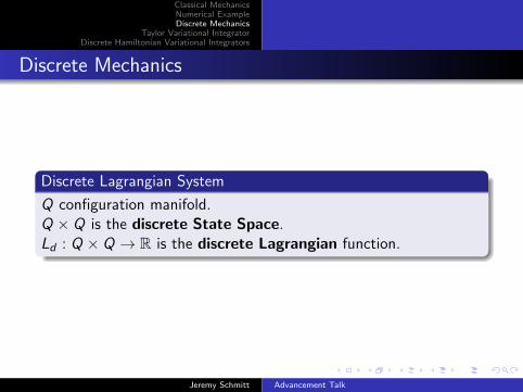
Discrete Mechanics
Discrete Lagrangian System
Q configuration manifold.Q × Q is the discrete State Space.Ld : Q × Q → R is the discrete Lagrangian function.
Jeremy Schmitt Advancement Talk

Classical MechanicsNumerical ExampleDiscrete Mechanics
Taylor Variational IntegratorDiscrete Hamiltonian Variational Integrators
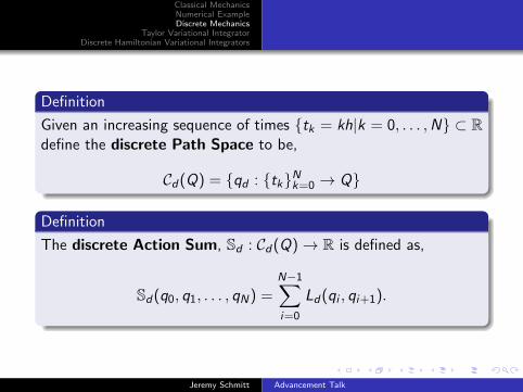
Definition
Given an increasing sequence of times {tk = kh|k = 0, . . . ,N} ⊂ Rdefine the discrete Path Space to be,
Cd(Q) = {qd : {tk}Nk=0 → Q}
Definition
The discrete Action Sum, Sd : Cd(Q)→ R is defined as,
Sd(q0, q1, . . . , qN) =N−1∑i=0
Ld(qi , qi+1).
Jeremy Schmitt Advancement Talk
Classical MechanicsNumerical ExampleDiscrete Mechanics
Taylor Variational IntegratorDiscrete Hamiltonian Variational Integrators
Definition
Given an increasing sequence of times {tk = kh|k = 0, . . . ,N} ⊂ Rdefine the discrete Path Space to be,
Cd(Q) = {qd : {tk}Nk=0 → Q}
Definition
The discrete Action Sum, Sd : Cd(Q)→ R is defined as,
Sd(q0, q1, . . . , qN) =N−1∑i=0
Ld(qi , qi+1).
Jeremy Schmitt Advancement Talk
Classical MechanicsNumerical ExampleDiscrete Mechanics
Taylor Variational IntegratorDiscrete Hamiltonian Variational Integrators
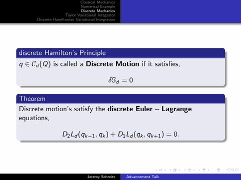
discrete Hamilton’s Principle
q ∈ Cd(Q) is called a Discrete Motion if it satisfies,
δSd = 0
Theorem
Discrete motion’s satisfy the discrete Euler − Lagrangeequations,
D2Ld(qk−1, qk) + D1Ld(qk , qk+1) = 0.
Jeremy Schmitt Advancement Talk
Classical MechanicsNumerical ExampleDiscrete Mechanics
Taylor Variational IntegratorDiscrete Hamiltonian Variational Integrators
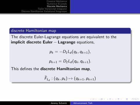
discrete Hamiltonian map
The discrete Euler-Lagrange equations are equivalent to theimplicit discrete Euler − Lagrange equations,
pk = −D1Ld(qk , qk+1),
pk+1 = D2Ld(qk , qk+1).
This defines the discrete Hamiltonian map,
FLd : (qk , pk) 7→ (qk+1, pk+1)
Jeremy Schmitt Advancement Talk
Classical MechanicsNumerical ExampleDiscrete Mechanics
Taylor Variational IntegratorDiscrete Hamiltonian Variational Integrators
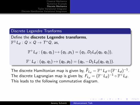
Discrete Legendre Tranforms
Define the discrete Legendre transforms,F±Ld : Q × Q → T ∗Q, as,
F+Ld : (q0, q1) 7→ (q1, p1) = (q1,D2Ld(q0, q1)),
F−Ld : (q0, q1) 7→ (q0, p0) = (q0,−D1Ld(q0, q1)).
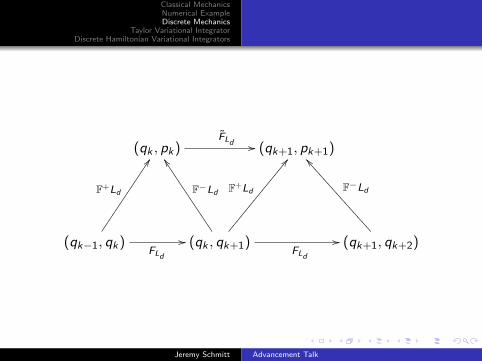
The discrete Hamiltonian map is given by, FLd = F+Ld ◦ (F−Ld)−1.The discrete Lagrangian map is given by, FLd = (F−Ld)−1 ◦ F+Ld .This leads to the following commutative diagram.
Jeremy Schmitt Advancement Talk
Classical MechanicsNumerical ExampleDiscrete Mechanics
Taylor Variational IntegratorDiscrete Hamiltonian Variational Integrators
(qk , pk)FLd // (qk+1, pk+1)
(qk−1, qk)
F+Ld
DD
FLd
// (qk , qk+1)FLd
//
F+Ld
BB��������������
F−Ld
ZZ4444444444444
(qk+1, qk+2)
F−Ld
]]<<<<<<<<<<<<<<<
Jeremy Schmitt Advancement Talk
Classical MechanicsNumerical ExampleDiscrete Mechanics
Taylor Variational IntegratorDiscrete Hamiltonian Variational Integrators
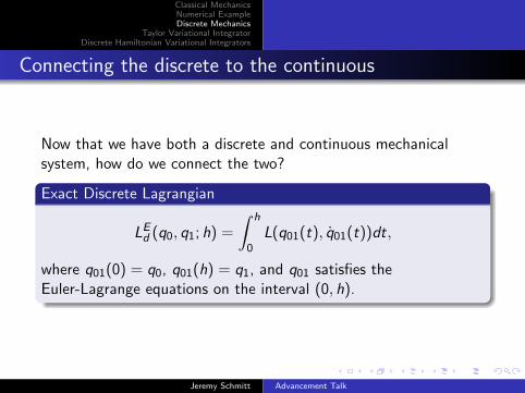
Connecting the discrete to the continuous
Now that we have both a discrete and continuous mechanicalsystem, how do we connect the two?
Exact Discrete Lagrangian
LEd (q0, q1; h) =
∫ h
0L(q01(t), q01(t))dt,
where q01(0) = q0, q01(h) = q1, and q01 satisfies theEuler-Lagrange equations on the interval (0, h).
Jeremy Schmitt Advancement Talk
Classical MechanicsNumerical ExampleDiscrete Mechanics
Taylor Variational IntegratorDiscrete Hamiltonian Variational Integrators
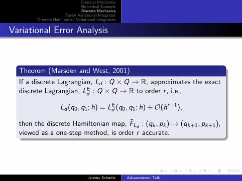
Variational Error Analysis
Theorem (Marsden and West, 2001)
If a discrete Lagrangian, Ld : Q × Q → R, approximates the exactdiscrete Lagrangian, LE
d : Q × Q → R to order r , i.e.,
Ld(q0, q1; h) = LEd (q0, q1; h) +O(hr+1),
then the discrete Hamiltonian map, FLd : (qk , pk) 7→ (qk+1, pk+1),viewed as a one-step method, is order r accurate.
Jeremy Schmitt Advancement Talk
Classical MechanicsNumerical ExampleDiscrete Mechanics
Taylor Variational IntegratorDiscrete Hamiltonian Variational Integrators
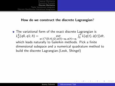
How do we construct the discrete Lagrangian?
The variational form of the exact discrete Lagrangian isLEd (q0, q1; h) = ext
q∈C2([0,h],Q),q(0)=q0,q(h)=q1
∫ h0 L(q(t), q(t))dt,
which leads naturally to Galerkin methods. Pick a finitedimensional subspace and a numerical quadrature method tobuild the discrete Lagrangian.(Leok, Shingel)
The type-I generating function form of the exact discreteLagrangian is LE
d (q0, q1; h) =∫ h
0 L(q01(t), q01(t))dt, whereq01(0) = q0, q01(h) = q1, and q01 satisfies the Euler-Lagrangeequation in (0, h). Pick a one-step method, apply the shootingmethod to the Euler-Lagrange BVP, and use a quadrature ruleto generate the discrete Lagrangian.(Leok, Shingel)
Jeremy Schmitt Advancement Talk
Classical MechanicsNumerical ExampleDiscrete Mechanics
Taylor Variational IntegratorDiscrete Hamiltonian Variational Integrators
Prolongate the Euler-Lagrange vector field, and then apply acollocation method using Hermite interpolating polynomialsto approximate values of q and q satisfying theEuler-Lagrange BVP. Combing these with a quadrature ruleyields a discrete Lagrangian.(Leok, Shingel)
Prolongate the Euler-Lagrange vector field, and use this toconstruct Taylor’s method. Find the initial velocity by solvingan inverse problem, and then apply a quadrature rule to createa discrete Lagrangian.
Jeremy Schmitt Advancement Talk

Classical MechanicsNumerical ExampleDiscrete Mechanics
Taylor Variational IntegratorDiscrete Hamiltonian Variational Integrators
Outline
1 Classical Mechanics
2 Numerical Example
3 Discrete Mechanics
4 Taylor Variational Integrator
5 Discrete Hamiltonian Variational Integrators
Jeremy Schmitt Advancement Talk
Classical MechanicsNumerical ExampleDiscrete Mechanics
Taylor Variational IntegratorDiscrete Hamiltonian Variational Integrators
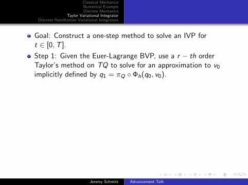
Goal: Construct a one-step method to solve an IVP fort ∈ [0,T ].
Step 1: Given the Euer-Lagrange BVP, use a r − th orderTaylor’s method on TQ to solve for an approximation to v0
implicitly defined by q1 = πQ ◦ Φh(q0, v0).
Step 2: Combine v0 with the r − th order Taylor’s method togenerate the quadrature points to define our discreteLagrangian.
Step 3: Apply the implicit Euler-Lagrange equations to thediscrete Lagrangian to generate the one-step method.
pk = −D1Ld(qk , qk+1),
pk+1 = D2Ld(qk , qk+1).
Jeremy Schmitt Advancement Talk
Classical MechanicsNumerical ExampleDiscrete Mechanics
Taylor Variational IntegratorDiscrete Hamiltonian Variational Integrators
Goal: Construct a one-step method to solve an IVP fort ∈ [0,T ].
Step 1: Given the Euer-Lagrange BVP, use a r − th orderTaylor’s method on TQ to solve for an approximation to v0
implicitly defined by q1 = πQ ◦ Φh(q0, v0).
Step 2: Combine v0 with the r − th order Taylor’s method togenerate the quadrature points to define our discreteLagrangian.
Step 3: Apply the implicit Euler-Lagrange equations to thediscrete Lagrangian to generate the one-step method.
pk = −D1Ld(qk , qk+1),
pk+1 = D2Ld(qk , qk+1).
Jeremy Schmitt Advancement Talk
Classical MechanicsNumerical ExampleDiscrete Mechanics
Taylor Variational IntegratorDiscrete Hamiltonian Variational Integrators
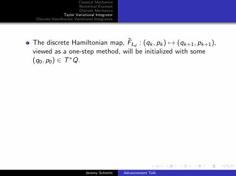
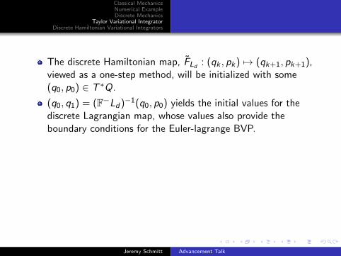
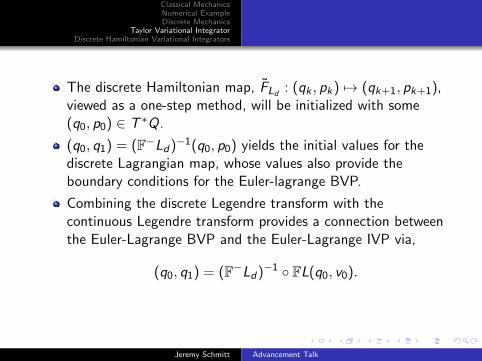
The discrete Hamiltonian map, FLd : (qk , pk) 7→ (qk+1, pk+1),viewed as a one-step method, will be initialized with some(q0, p0) ∈ T ∗Q.
(q0, q1) = (F−Ld)−1(q0, p0) yields the initial values for thediscrete Lagrangian map, whose values also provide theboundary conditions for the Euler-lagrange BVP.
Combining the discrete Legendre transform with thecontinuous Legendre transform provides a connection betweenthe Euler-Lagrange BVP and the Euler-Lagrange IVP via,
(q0, q1) = (F−Ld)−1 ◦ FL(q0, v0).
Jeremy Schmitt Advancement Talk
Classical MechanicsNumerical ExampleDiscrete Mechanics
Taylor Variational IntegratorDiscrete Hamiltonian Variational Integrators
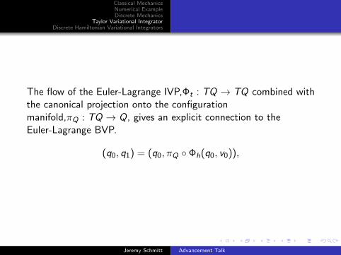
The flow of the Euler-Lagrange IVP,Φt : TQ → TQ combined withthe canonical projection onto the configurationmanifold,πQ : TQ → Q, gives an explicit connection to theEuler-Lagrange BVP.
(q0, q1) = (q0, πQ ◦ Φh(q0, v0)),
Jeremy Schmitt Advancement Talk
Classical MechanicsNumerical ExampleDiscrete Mechanics
Taylor Variational IntegratorDiscrete Hamiltonian Variational Integrators
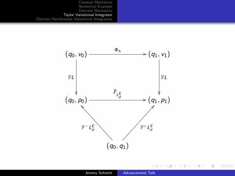
(q0, v0)
FL
��
Φh // (q1, v1)
FL
��(q0, p0)
FLEd // (q1, p1)
(q0, q1)
F−LEd
]]<<<<<<<<<<<<<<<
F+LEd
AA���������������
Jeremy Schmitt Advancement Talk
Classical MechanicsNumerical ExampleDiscrete Mechanics
Taylor Variational IntegratorDiscrete Hamiltonian Variational Integrators
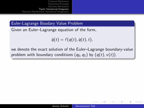
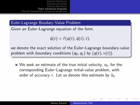
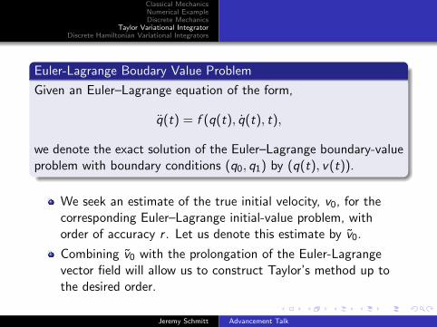
Euler-Lagrange Boudary Value Problem
Given an Euler–Lagrange equation of the form,
q(t) = f (q(t), q(t), t),
we denote the exact solution of the Euler–Lagrange boundary-valueproblem with boundary conditions (q0, q1) by (q(t), v(t)).
We seek an estimate of the true initial velocity, v0, for thecorresponding Euler–Lagrange initial-value problem, withorder of accuracy r . Let us denote this estimate by v0.
Combining v0 with the prolongation of the Euler-Lagrangevector field will allow us to construct Taylor’s method up tothe desired order.
Jeremy Schmitt Advancement Talk
Classical MechanicsNumerical ExampleDiscrete Mechanics
Taylor Variational IntegratorDiscrete Hamiltonian Variational Integrators
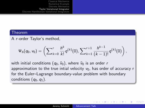
Theorem
A r -order Taylor’s method,
Ψh(q0, v0) =
(∑r
k=0
hk
k!q(k)(0),
∑r+1
k=1
hk−1
(k − 1)!q(k)(0)
),
with initial conditions (q0, v0), where v0 is an order rapproximation to the true intial velocity v0, has order of accuracy rfor the Euler–Lagrange boundary-value problem with boundaryconditions (q0, q1).
Jeremy Schmitt Advancement Talk
Classical MechanicsNumerical ExampleDiscrete Mechanics
Taylor Variational IntegratorDiscrete Hamiltonian Variational Integrators
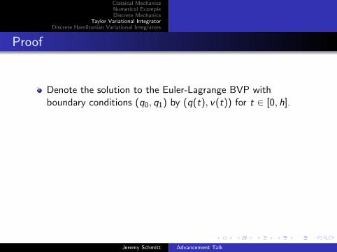
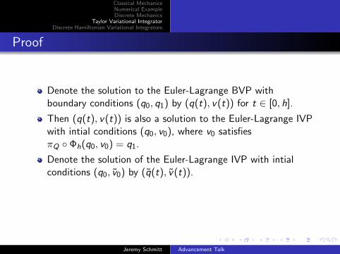
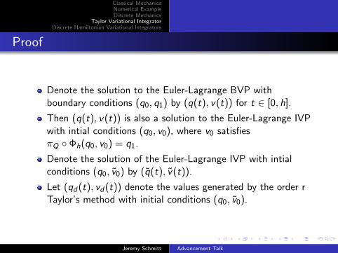
Proof
Denote the solution to the Euler-Lagrange BVP withboundary conditions (q0, q1) by (q(t), v(t)) for t ∈ [0, h].
Then (q(t), v(t)) is also a solution to the Euler-Lagrange IVPwith intial conditions (q0, v0), where v0 satisfiesπQ ◦ Φh(q0, v0) = q1.
Denote the solution of the Euler-Lagrange IVP with intialconditions (q0, v0) by (q(t), v(t)).
Let (qd(t), vd(t)) denote the values generated by the order rTaylor’s method with initial conditions (q0, v0).
Jeremy Schmitt Advancement Talk
Classical MechanicsNumerical ExampleDiscrete Mechanics
Taylor Variational IntegratorDiscrete Hamiltonian Variational Integrators
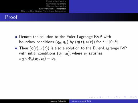
Proof
Denote the solution to the Euler-Lagrange BVP withboundary conditions (q0, q1) by (q(t), v(t)) for t ∈ [0, h].
Then (q(t), v(t)) is also a solution to the Euler-Lagrange IVPwith intial conditions (q0, v0), where v0 satisfiesπQ ◦ Φh(q0, v0) = q1.
Denote the solution of the Euler-Lagrange IVP with intialconditions (q0, v0) by (q(t), v(t)).
Let (qd(t), vd(t)) denote the values generated by the order rTaylor’s method with initial conditions (q0, v0).
Jeremy Schmitt Advancement Talk

Classical MechanicsNumerical ExampleDiscrete Mechanics
Taylor Variational IntegratorDiscrete Hamiltonian Variational Integrators
Proof
Let M be the Lipschitz constant with respect to initial velocity ofthe well-posed Euler-Lagrange IVP. Then,
‖(q(t), v(t))− (q(t), v(t))‖ ≤ M‖v0 − v0‖ ≤ O(hr+1).
Combining this inequality with our r -order method yields,
‖(q(t), v(t))− (qd(t), vd(t))‖= ‖(q(t), v(t))− (q(t), v(t)) + (q(t), v(t))− (qd(t), vd(t))‖≤ ‖(q(t), v(t))− (q(t), v(t))‖+ ‖(q(t), v(t))− (qd(t), vd(t))‖≤ O(hr+1).
Jeremy Schmitt Advancement Talk

Classical MechanicsNumerical ExampleDiscrete Mechanics
Taylor Variational IntegratorDiscrete Hamiltonian Variational Integrators
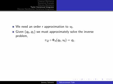
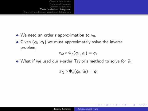
We need an order r approximation to v0.
Given (q0, q1) we must approximately solve the inverseproblem,
πQ ◦ Φh(q0, v0) = q1.
What if we used our r-order Taylor’s method to solve for v0
πQ ◦Ψh(q0, v0) = q1
Jeremy Schmitt Advancement Talk
Classical MechanicsNumerical ExampleDiscrete Mechanics
Taylor Variational IntegratorDiscrete Hamiltonian Variational Integrators
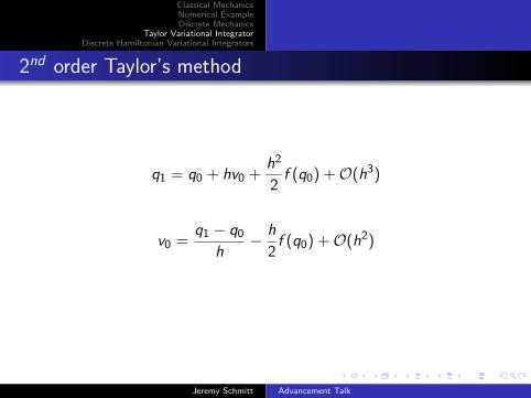
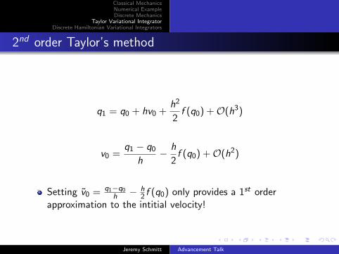
2nd order Taylor’s method
q1 = q0 + hv0 +h2
2f (q0) +O(h3)
v0 =q1 − q0
h− h
2f (q0) +O(h2)
Setting v0 = q1−q0h − h
2 f (q0) only provides a 1st orderapproximation to the intitial velocity!
Jeremy Schmitt Advancement Talk
Classical MechanicsNumerical ExampleDiscrete Mechanics
Taylor Variational IntegratorDiscrete Hamiltonian Variational Integrators
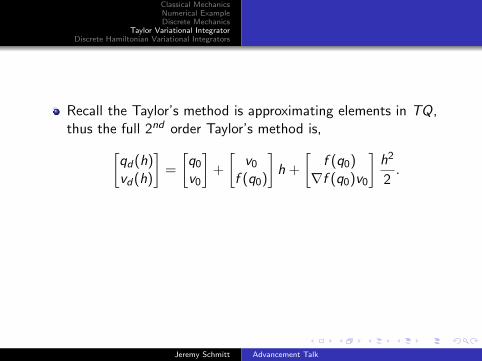
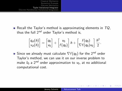
Recall the Taylor’s method is approximating elements in TQ,thus the full 2nd order Taylor’s method is,[
qd(h)vd(h)
]=
[q0
v0
]+
[v0
f (q0)
]h +
[f (q0)∇f (q0)v0
]h2
2.
Since we already must calculate ∇f (q0) for the 2nd orderTaylor’s method, we can use it on our inverse problem tomake v0 a 2nd order approximation to v0, at no additionalcomputational cost.
Jeremy Schmitt Advancement Talk
Classical MechanicsNumerical ExampleDiscrete Mechanics
Taylor Variational IntegratorDiscrete Hamiltonian Variational Integrators
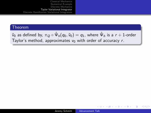
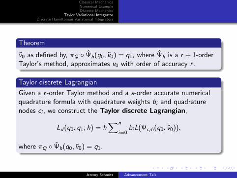
Theorem
v0 as defined by, πQ ◦ Ψh(q0, v0) = q1, where Ψh is a r + 1-orderTaylor’s method, approximates v0 with order of accuracy r .
Taylor discrete Lagrangian
Given a r -order Taylor method and a s-order accurate numericalquadrature formula with quadrature weights bi and quadraturenodes ci , we construct the Taylor discrete Lagrangian,
Ld(q0, q1; h) = h∑n
i=0biL(Ψcih(q0, v0)),
where πQ ◦ Ψh(q0, v0) = q1.
Jeremy Schmitt Advancement Talk
Classical MechanicsNumerical ExampleDiscrete Mechanics
Taylor Variational IntegratorDiscrete Hamiltonian Variational Integrators
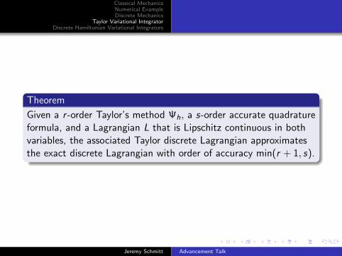
Theorem
Given a r -order Taylor’s method Ψh, a s-order accurate quadratureformula, and a Lagrangian L that is Lipschitz continuous in bothvariables, the associated Taylor discrete Lagrangian approximatesthe exact discrete Lagrangian with order of accuracy min(r + 1, s).
Jeremy Schmitt Advancement Talk
Classical MechanicsNumerical ExampleDiscrete Mechanics
Taylor Variational IntegratorDiscrete Hamiltonian Variational Integrators
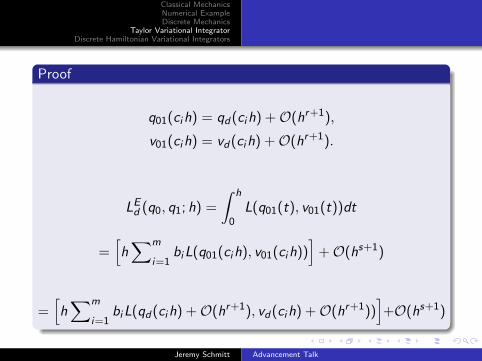
Proof
q01(cih) = qd(cih) +O(hr+1),
v01(cih) = vd(cih) +O(hr+1).
LEd (q0, q1; h) =
∫ h
0L(q01(t), v01(t))dt
=[h∑m
i=1biL(q01(cih), v01(cih))
]+O(hs+1)
=[h∑m
i=1biL(qd(cih) +O(hr+1), vd(cih) +O(hr+1))
]+O(hs+1)
Jeremy Schmitt Advancement Talk
Classical MechanicsNumerical ExampleDiscrete Mechanics
Taylor Variational IntegratorDiscrete Hamiltonian Variational Integrators
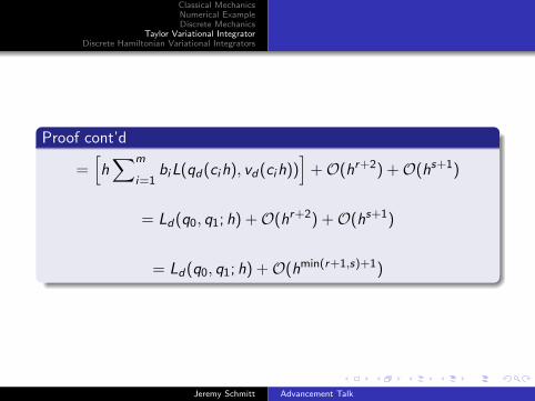
Proof cont’d
=[h∑m
i=1biL(qd(cih), vd(cih))
]+O(hr+2) +O(hs+1)
= Ld(q0, q1; h) +O(hr+2) +O(hs+1)
= Ld(q0, q1; h) +O(hmin(r+1,s)+1)
Jeremy Schmitt Advancement Talk
Classical MechanicsNumerical ExampleDiscrete Mechanics
Taylor Variational IntegratorDiscrete Hamiltonian Variational Integrators
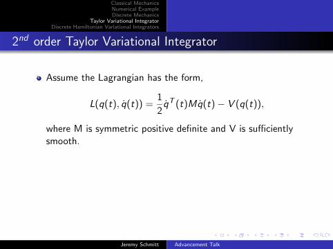
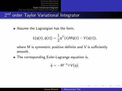
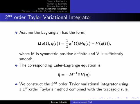
2nd order Taylor Variational Integrator
Assume the Lagrangian has the form,
L(q(t), q(t)) =1
2qT (t)Mq(t)− V (q(t)),
where M is symmetric positive definite and V is sufficientlysmooth.
The corresponding Euler-Lagrange equation is,
q = −M−1OV (q).
We construct the 2nd order Taylor variational integrator usinga 1st order Taylor’s method combined with the trapezoid rule.
Jeremy Schmitt Advancement Talk
Classical MechanicsNumerical ExampleDiscrete Mechanics
Taylor Variational IntegratorDiscrete Hamiltonian Variational Integrators
2nd order Taylor Variational Integrator
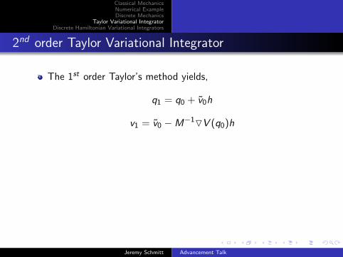
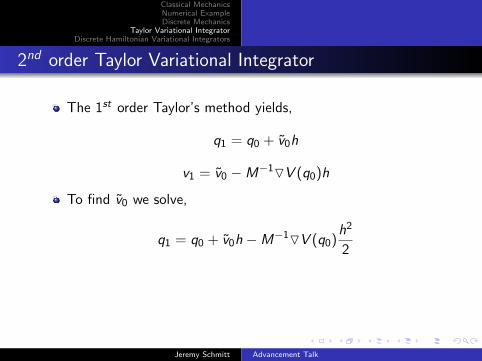
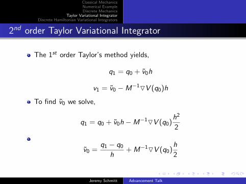
The 1st order Taylor’s method yields,
q1 = q0 + v0h
v1 = v0 −M−1OV (q0)h
To find v0 we solve,
q1 = q0 + v0h −M−1OV (q0)h2
2
v0 =q1 − q0
h+ M−1OV (q0)
h
2
Jeremy Schmitt Advancement Talk
Classical MechanicsNumerical ExampleDiscrete Mechanics
Taylor Variational IntegratorDiscrete Hamiltonian Variational Integrators
2nd order Taylor Variational Integrator
The 1st order Taylor’s method yields,
q1 = q0 + v0h
v1 = v0 −M−1OV (q0)h
To find v0 we solve,
q1 = q0 + v0h −M−1OV (q0)h2
2
v0 =q1 − q0
h+ M−1OV (q0)
h
2
Jeremy Schmitt Advancement Talk
Classical MechanicsNumerical ExampleDiscrete Mechanics
Taylor Variational IntegratorDiscrete Hamiltonian Variational Integrators
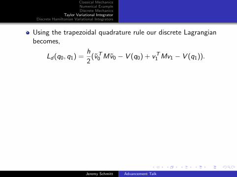
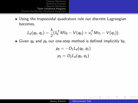
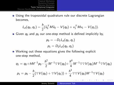
Using the trapezoidal quadrature rule our discrete Lagrangianbecomes,
Ld(q0, q1) =h
2(vT
0 Mv0 − V (q0) + vT1 Mv1 − V (q1)).
Given q0 and p0 our one-step method is defined implicitly by,
p0 = −D1Ld(q0, q1)
p1 = D2Ld(q0, q1)
Working out these equations gives the following explicitone-step method,
q1 = q0+hM−1p0−h2
2M−1OV (q0)+
h4
4M−1OOV (q0)M−1OV (q0)
p1 = p0 −h
2(OV (q0) + OV (q1)) +
h3
4OOV (q0)M−1OV (q0)
Jeremy Schmitt Advancement Talk
Classical MechanicsNumerical ExampleDiscrete Mechanics
Taylor Variational IntegratorDiscrete Hamiltonian Variational Integrators
Using the trapezoidal quadrature rule our discrete Lagrangianbecomes,
Ld(q0, q1) =h
2(vT
0 Mv0 − V (q0) + vT1 Mv1 − V (q1)).
Given q0 and p0 our one-step method is defined implicitly by,
p0 = −D1Ld(q0, q1)
p1 = D2Ld(q0, q1)
Working out these equations gives the following explicitone-step method,
q1 = q0+hM−1p0−h2
2M−1OV (q0)+
h4
4M−1OOV (q0)M−1OV (q0)
p1 = p0 −h
2(OV (q0) + OV (q1)) +
h3
4OOV (q0)M−1OV (q0)
Jeremy Schmitt Advancement Talk

Classical MechanicsNumerical ExampleDiscrete Mechanics
Taylor Variational IntegratorDiscrete Hamiltonian Variational Integrators
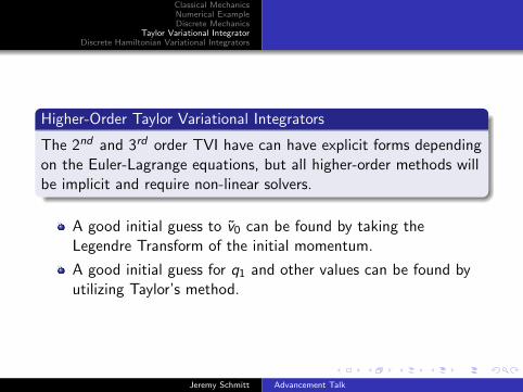
Higher-Order Taylor Variational Integrators
The 2nd and 3rd order TVI have can have explicit forms dependingon the Euler-Lagrange equations, but all higher-order methods willbe implicit and require non-linear solvers.
A good initial guess to v0 can be found by taking theLegendre Transform of the initial momentum.
A good initial guess for q1 and other values can be found byutilizing Taylor’s method.
Jeremy Schmitt Advancement Talk

Classical MechanicsNumerical ExampleDiscrete Mechanics
Taylor Variational IntegratorDiscrete Hamiltonian Variational Integrators
Higher-Order Taylor Variational Integrators
The 2nd and 3rd order TVI have can have explicit forms dependingon the Euler-Lagrange equations, but all higher-order methods willbe implicit and require non-linear solvers.
A good initial guess to v0 can be found by taking theLegendre Transform of the initial momentum.
A good initial guess for q1 and other values can be found byutilizing Taylor’s method.
Jeremy Schmitt Advancement Talk
Classical MechanicsNumerical ExampleDiscrete Mechanics
Taylor Variational IntegratorDiscrete Hamiltonian Variational Integrators
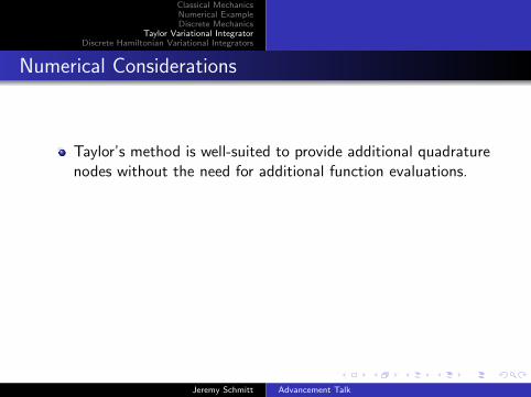
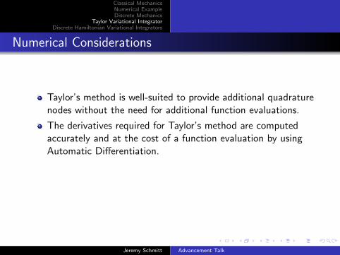
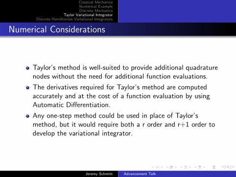
Numerical Considerations
Taylor’s method is well-suited to provide additional quadraturenodes without the need for additional function evaluations.
The derivatives required for Taylor’s method are computedaccurately and at the cost of a function evaluation by usingAutomatic Differentiation.
Any one-step method could be used in place of Taylor’smethod, but it would require both a r order and r+1 order todevelop the variational integrator.
Jeremy Schmitt Advancement Talk
Classical MechanicsNumerical ExampleDiscrete Mechanics
Taylor Variational IntegratorDiscrete Hamiltonian Variational Integrators
Numerical Considerations
Taylor’s method is well-suited to provide additional quadraturenodes without the need for additional function evaluations.
The derivatives required for Taylor’s method are computedaccurately and at the cost of a function evaluation by usingAutomatic Differentiation.
Any one-step method could be used in place of Taylor’smethod, but it would require both a r order and r+1 order todevelop the variational integrator.
Jeremy Schmitt Advancement Talk

Classical MechanicsNumerical ExampleDiscrete Mechanics
Taylor Variational IntegratorDiscrete Hamiltonian Variational Integrators
Outline
1 Classical Mechanics
2 Numerical Example
3 Discrete Mechanics
4 Taylor Variational Integrator
5 Discrete Hamiltonian Variational Integrators
Jeremy Schmitt Advancement Talk
Classical MechanicsNumerical ExampleDiscrete Mechanics
Taylor Variational IntegratorDiscrete Hamiltonian Variational Integrators
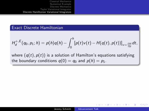
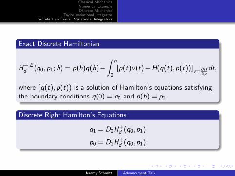
Exact Discrete Hamiltonian
H+,Ed (q0, p1; h) = p(h)q(h)−
∫ h
0[p(t)v(t)−H(q(t), p(t))]v= ∂H
∂pdt,
where (q(t), p(t)) is a solution of Hamilton’s equations satisfyingthe boundary conditions q(0) = q0 and p(h) = p1.
Discrete Right Hamilton’s Equations
q1 = D2H+d (q0, p1)
p0 = D1H+d (q0, p1)
Jeremy Schmitt Advancement Talk
Classical MechanicsNumerical ExampleDiscrete Mechanics
Taylor Variational IntegratorDiscrete Hamiltonian Variational Integrators
If the Lagrangian is degenerate, then the Legendre transformis not invertible, and it may make more sense to approach theproblem from the Hamiltonian side.
Letting h→ 0 causes a breakdown in the well-posedness of aBVP, with Dirichlet boundary conditions q(0) = q0 andq(h) = q1, as the initial velocity becomes unbounded.
Letting h→ 0 does not cause this singularity when theboundary conditions are q(0) = q0 and p(h) = p1.
Jeremy Schmitt Advancement Talk

Classical MechanicsNumerical ExampleDiscrete Mechanics
Taylor Variational IntegratorDiscrete Hamiltonian Variational Integrators
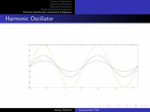
Harmonic Oscillator
Consider the harmonic oscillator given by the Euler-Lagrange BVP,
q(t) = −kx ,
where q(0) = 0 and q( π√k
) = 0. This BVP does not have a unique
solution!
Jeremy Schmitt Advancement Talk
Classical MechanicsNumerical ExampleDiscrete Mechanics
Taylor Variational IntegratorDiscrete Hamiltonian Variational Integrators
Harmonic Oscillator
Jeremy Schmitt Advancement Talk
Classical MechanicsNumerical ExampleDiscrete Mechanics
Taylor Variational IntegratorDiscrete Hamiltonian Variational Integrators
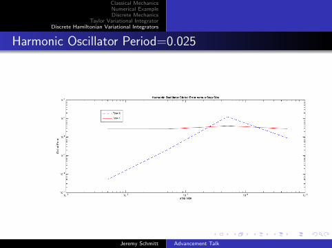
Harmonic Oscillator Period=0.025
Jeremy Schmitt Advancement Talk
Classical MechanicsNumerical ExampleDiscrete Mechanics
Taylor Variational IntegratorDiscrete Hamiltonian Variational Integrators
Discrete variational Hamitonian mechanics has been developedin papers by (Lall, West 2006) and (Leok, Zhang 2011).
The exact discrete Hamiltonian is a type 2 generating functionof the exact flow of Hamilton’s equations.(Leok, Zhang 2011)
The map defined by constructing a discrete right Hamitonianand applying the discrete right Hamilton’s equations issymplectic and preserves momentum maps. (Leok, Zhang2011)
Jeremy Schmitt Advancement Talk
Classical MechanicsNumerical ExampleDiscrete Mechanics
Taylor Variational IntegratorDiscrete Hamiltonian Variational Integrators
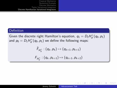
Definition
Given the discrete right Hamilton’s equation, q1 = D2H+d (q0, p1)
and p0 = D1H+d (q0, p1) we define the following maps:
FH+d
: (qk , pk) 7→ (qk+1, pk+1)
FH+d
: (qk , pk+1) 7→ (qk+1, pk+2)
Jeremy Schmitt Advancement Talk
Classical MechanicsNumerical ExampleDiscrete Mechanics
Taylor Variational IntegratorDiscrete Hamiltonian Variational Integrators
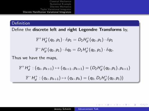
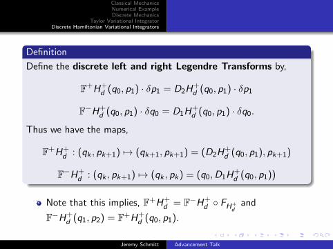
Definition
Define the discrete left and right Legendre Transforms by,
F+H+d (q0, p1) · δp1 = D2H+
d (q0, p1) · δp1
F−H+d (q0, p1) · δq0 = D1H+
d (q0, p1) · δq0.
Thus we have the maps,
F+H+d : (qk , pk+1) 7→ (qk+1, pk+1) = (D2H+
d (q0, p1), pk+1)
F−H+d : (qk , pk+1) 7→ (qk , pk) = (q0,D1H+
d (q0, p1))
Note that this implies, F+H+d = F−H+
d ◦ FH+d
and
F−H+d (q1, p2) = F+H+
d (q0, p1).
Jeremy Schmitt Advancement Talk
Classical MechanicsNumerical ExampleDiscrete Mechanics
Taylor Variational IntegratorDiscrete Hamiltonian Variational Integrators
Definition
Define the discrete left and right Legendre Transforms by,
F+H+d (q0, p1) · δp1 = D2H+
d (q0, p1) · δp1
F−H+d (q0, p1) · δq0 = D1H+
d (q0, p1) · δq0.
Thus we have the maps,
F+H+d : (qk , pk+1) 7→ (qk+1, pk+1) = (D2H+
d (q0, p1), pk+1)
F−H+d : (qk , pk+1) 7→ (qk , pk) = (q0,D1H+
d (q0, p1))
Note that this implies, F+H+d = F−H+
d ◦ FH+d
and
F−H+d (q1, p2) = F+H+
d (q0, p1).
Jeremy Schmitt Advancement Talk
Classical MechanicsNumerical ExampleDiscrete Mechanics
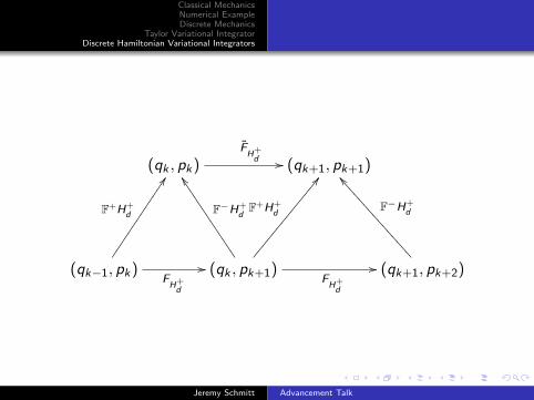
Taylor Variational IntegratorDiscrete Hamiltonian Variational Integrators
(qk , pk)FH+d // (qk+1, pk+1)
(qk−1, pk)
F+H+d
DD
FH+d
// (qk , pk+1)FH+d
//
F+H+d
BB��������������
F−H+d
ZZ4444444444444
(qk+1, pk+2)
F−H+d
]]<<<<<<<<<<<<<<<
Jeremy Schmitt Advancement Talk
Classical MechanicsNumerical ExampleDiscrete Mechanics
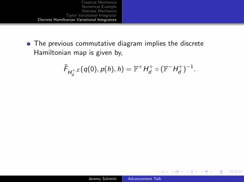
Taylor Variational IntegratorDiscrete Hamiltonian Variational Integrators
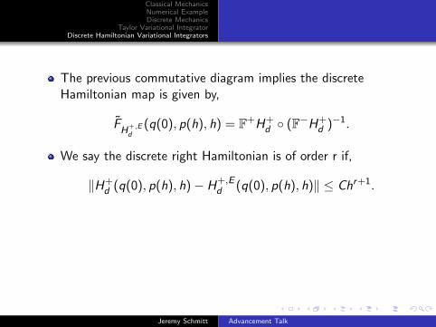
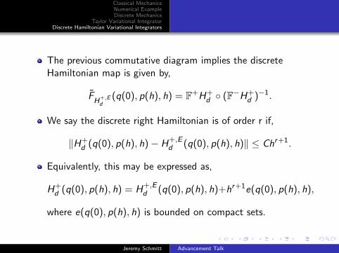
The previous commutative diagram implies the discreteHamiltonian map is given by,
FH+,Ed
(q(0), p(h), h) = F+H+d ◦ (F−H+
d )−1.
We say the discrete right Hamiltonian is of order r if,
‖H+d (q(0), p(h), h)− H+,E
d (q(0), p(h), h)‖ ≤ Chr+1.
Equivalently, this may be expressed as,
H+d (q(0), p(h), h) = H+,E
d (q(0), p(h), h)+hr+1e(q(0), p(h), h),
where e(q(0), p(h), h) is bounded on compact sets.
Jeremy Schmitt Advancement Talk
Classical MechanicsNumerical ExampleDiscrete Mechanics
Taylor Variational IntegratorDiscrete Hamiltonian Variational Integrators
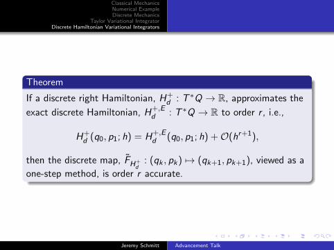
Theorem
If a discrete right Hamiltonian, H+d : T ∗Q → R, approximates the
exact discrete Hamiltonian, H+,Ed : T ∗Q → R to order r , i.e.,
H+d (q0, p1; h) = H+,E
d (q0, p1; h) +O(hr+1),
then the discrete map, FH+d
: (qk , pk) 7→ (qk+1, pk+1), viewed as a
one-step method, is order r accurate.
Jeremy Schmitt Advancement Talk
Classical MechanicsNumerical ExampleDiscrete Mechanics
Taylor Variational IntegratorDiscrete Hamiltonian Variational Integrators
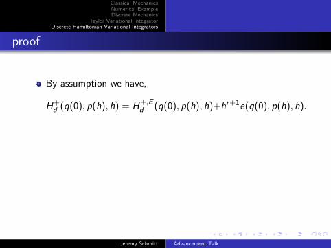
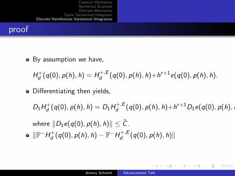
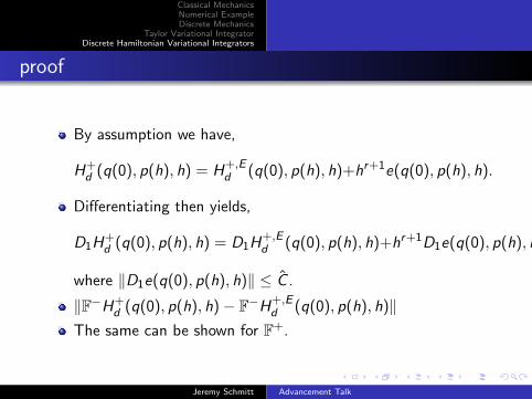
proof
By assumption we have,
H+d (q(0), p(h), h) = H+,E
d (q(0), p(h), h)+hr+1e(q(0), p(h), h).
Differentiating then yields,
D1H+d (q(0), p(h), h) = D1H+,E
d (q(0), p(h), h)+hr+1D1e(q(0), p(h), h),
where ‖D1e(q(0), p(h), h)‖ ≤ C .
‖F−H+d (q(0), p(h), h)− F−H+,E
d (q(0), p(h), h)‖The same can be shown for F+.
Jeremy Schmitt Advancement Talk

Classical MechanicsNumerical ExampleDiscrete Mechanics
Taylor Variational IntegratorDiscrete Hamiltonian Variational Integrators
proof
By assumption we have,
H+d (q(0), p(h), h) = H+,E
d (q(0), p(h), h)+hr+1e(q(0), p(h), h).
Differentiating then yields,
D1H+d (q(0), p(h), h) = D1H+,E
d (q(0), p(h), h)+hr+1D1e(q(0), p(h), h),
where ‖D1e(q(0), p(h), h)‖ ≤ C .
‖F−H+d (q(0), p(h), h)− F−H+,E
d (q(0), p(h), h)‖The same can be shown for F+.
Jeremy Schmitt Advancement Talk
Classical MechanicsNumerical ExampleDiscrete Mechanics
Taylor Variational IntegratorDiscrete Hamiltonian Variational Integrators
proof
By assumption we have,
H+d (q(0), p(h), h) = H+,E
d (q(0), p(h), h)+hr+1e(q(0), p(h), h).
Differentiating then yields,
D1H+d (q(0), p(h), h) = D1H+,E
d (q(0), p(h), h)+hr+1D1e(q(0), p(h), h),
where ‖D1e(q(0), p(h), h)‖ ≤ C .
‖F−H+d (q(0), p(h), h)− F−H+,E
d (q(0), p(h), h)‖
The same can be shown for F+.
Jeremy Schmitt Advancement Talk
Classical MechanicsNumerical ExampleDiscrete Mechanics
Taylor Variational IntegratorDiscrete Hamiltonian Variational Integrators
proof
By assumption we have,
H+d (q(0), p(h), h) = H+,E
d (q(0), p(h), h)+hr+1e(q(0), p(h), h).
Differentiating then yields,
D1H+d (q(0), p(h), h) = D1H+,E
d (q(0), p(h), h)+hr+1D1e(q(0), p(h), h),
where ‖D1e(q(0), p(h), h)‖ ≤ C .
‖F−H+d (q(0), p(h), h)− F−H+,E
d (q(0), p(h), h)‖The same can be shown for F+.
Jeremy Schmitt Advancement Talk
Classical MechanicsNumerical ExampleDiscrete Mechanics
Taylor Variational IntegratorDiscrete Hamiltonian Variational Integrators
proof
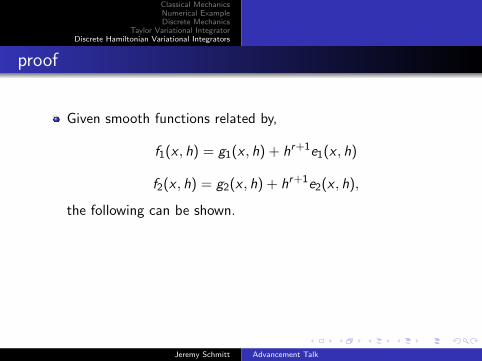
Given smooth functions related by,
f1(x , h) = g1(x , h) + hr+1e1(x , h)
f2(x , h) = g2(x , h) + hr+1e2(x , h),
the following can be shown.
f2(f1(x , h), h) = g2(g1(x , h), h) + hr+1e12(x , h)
f −11 (y , h) = g−1
1 (y , h) + hr+1e1(y , h)
Jeremy Schmitt Advancement Talk

Classical MechanicsNumerical ExampleDiscrete Mechanics
Taylor Variational IntegratorDiscrete Hamiltonian Variational Integrators
proof
Given smooth functions related by,
f1(x , h) = g1(x , h) + hr+1e1(x , h)
f2(x , h) = g2(x , h) + hr+1e2(x , h),
the following can be shown.
f2(f1(x , h), h) = g2(g1(x , h), h) + hr+1e12(x , h)
f −11 (y , h) = g−1
1 (y , h) + hr+1e1(y , h)
Jeremy Schmitt Advancement Talk
Classical MechanicsNumerical ExampleDiscrete Mechanics
Taylor Variational IntegratorDiscrete Hamiltonian Variational Integrators
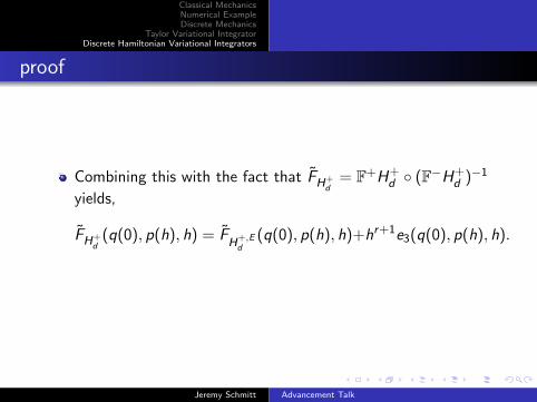
proof
Combining this with the fact that FH+d
= F+H+d ◦ (F−H+
d )−1
yields,
FH+d
(q(0), p(h), h) = FH+,Ed
(q(0), p(h), h)+hr+1e3(q(0), p(h), h).
Jeremy Schmitt Advancement Talk
Classical MechanicsNumerical ExampleDiscrete Mechanics
Taylor Variational IntegratorDiscrete Hamiltonian Variational Integrators
TVI on the Hamiltonian side
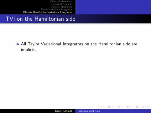
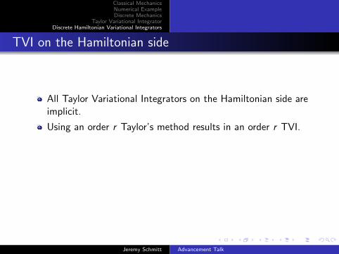
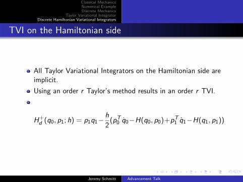
All Taylor Variational Integrators on the Hamiltonian side areimplicit.
Using an order r Taylor’s method results in an order r TVI.
H+d (q0, p1; h) = p1q1−
h
2(pT
0 q0−H(q0, p0)+pT1 q1−H(q1, p1))
Jeremy Schmitt Advancement Talk
Classical MechanicsNumerical ExampleDiscrete Mechanics
Taylor Variational IntegratorDiscrete Hamiltonian Variational Integrators
TVI on the Hamiltonian side
All Taylor Variational Integrators on the Hamiltonian side areimplicit.
Using an order r Taylor’s method results in an order r TVI.
H+d (q0, p1; h) = p1q1−
h
2(pT
0 q0−H(q0, p0)+pT1 q1−H(q1, p1))
Jeremy Schmitt Advancement Talk
Classical MechanicsNumerical ExampleDiscrete Mechanics
Taylor Variational IntegratorDiscrete Hamiltonian Variational Integrators
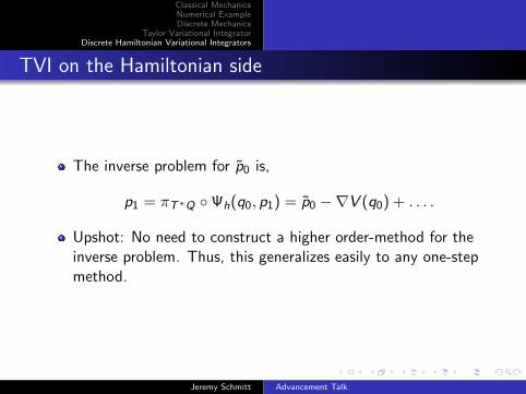
TVI on the Hamiltonian side
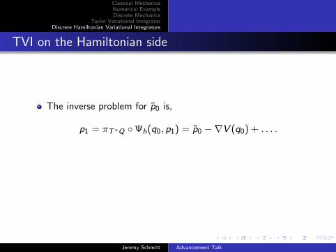
The inverse problem for p0 is,
p1 = πT∗Q ◦Ψh(q0, p1) = p0 −∇V (q0) + . . . .
Upshot: No need to construct a higher order-method for theinverse problem. Thus, this generalizes easily to any one-stepmethod.
Jeremy Schmitt Advancement Talk
Classical MechanicsNumerical ExampleDiscrete Mechanics
Taylor Variational IntegratorDiscrete Hamiltonian Variational Integrators
TVI on the Hamiltonian side
The inverse problem for p0 is,
p1 = πT∗Q ◦Ψh(q0, p1) = p0 −∇V (q0) + . . . .
Upshot: No need to construct a higher order-method for theinverse problem. Thus, this generalizes easily to any one-stepmethod.
Jeremy Schmitt Advancement Talk
Classical MechanicsNumerical ExampleDiscrete Mechanics
Taylor Variational IntegratorDiscrete Hamiltonian Variational Integrators
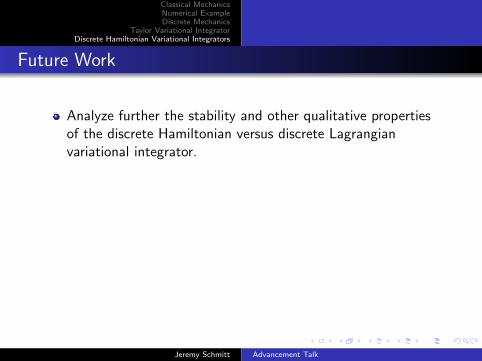
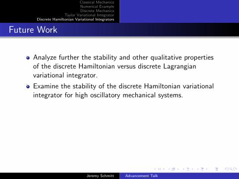
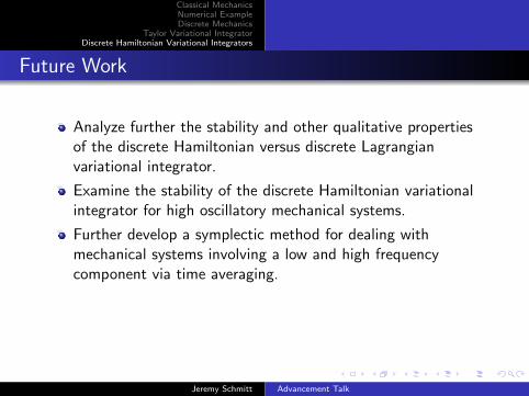
Future Work
Analyze further the stability and other qualitative propertiesof the discrete Hamiltonian versus discrete Lagrangianvariational integrator.
Examine the stability of the discrete Hamiltonian variationalintegrator for high oscillatory mechanical systems.
Further develop a symplectic method for dealing withmechanical systems involving a low and high frequencycomponent via time averaging.
Investigate the discretization of the boundary Lagrangian andpossibly a boundary Hamiltonian for multi-symplectic fieldtheories.
Jeremy Schmitt Advancement Talk
Classical MechanicsNumerical ExampleDiscrete Mechanics
Taylor Variational IntegratorDiscrete Hamiltonian Variational Integrators
Future Work
Analyze further the stability and other qualitative propertiesof the discrete Hamiltonian versus discrete Lagrangianvariational integrator.
Examine the stability of the discrete Hamiltonian variationalintegrator for high oscillatory mechanical systems.
Further develop a symplectic method for dealing withmechanical systems involving a low and high frequencycomponent via time averaging.
Investigate the discretization of the boundary Lagrangian andpossibly a boundary Hamiltonian for multi-symplectic fieldtheories.
Jeremy Schmitt Advancement Talk


![Introduction - CCoM Home · Schi [8] in the language of discrete mechanics and a discrete analogue of Jacobi’s solution to the discrete Hamilton{Jacobi equation. The remainder of](https://img.pdfslide.us/doc/110x75/5e7599fc9ca6a57ff15f08ee/introduction-ccom-home-schi-8-in-the-language-of-discrete-mechanics-and-a-discrete.jpg)


![[Donald W. Taylor] Fundamentals of Soil Mechanics](https://img.pdfslide.us/doc/110x75/55cf94b2550346f57ba3ce13/donald-w-taylor-fundamentals-of-soil-mechanics.jpg)


![[Donald W. Taylor] Fundamentals of Soil Mechanics(BookZa.org)](https://img.pdfslide.us/doc/110x75/55cf9830550346d03396205f/donald-w-taylor-fundamentals-of-soil-mechanicsbookzaorg.jpg)