2229198m_Merchant_ENG5059P_Thesis_2016

Propulsive efficiency of flapping foilsAn extension of the LDVM algorithm

By

Laura E. Merchant

Department of Aerospace EngineeringUniversity of Glasgow

This dissertation is submitted for the degree of Master of

Science in the School of Engineering.

Supervised by: Dr. Kiran Ramesh

August 2016

Word count: 15,053

D E C L A R AT I O N

I declare that the work in this dissertation was carried out in accordance with therequirements of the University of Glasgow’s Regulations and Code of Practiceas well as the requirements stated by the School of Engineering. This work hasnot been submitted for any other academic award. Except where indicated byspecific reference in the text, the work is the candidate’s own work. Work donein collaboration with, or with the assistance of, others, is indicated as such. Anyviews expressed in the dissertation are those of the author.

SIGNED: Laura Merchant DATE: 28/08/2016

i

A C K N O W L E D G E M E N T S

I would like to thank Dr. Kiran Ramesh for all of the helpful discussions and encouragementhe provided throughout the project. I am also grateful to the Scottish Funding Council forthe opportunity to further my education with a tuition grant.

iii

A B S T R A C T

This current work aims to extend pre-existing numerical models, namely the leading-edgesuction parameter(LESP)-modulated discrete-vortex method (LDVM, Ramesh et al. (2014))to include flexible bodies and apply the method to investigate the enhancement (or dimin-ishment) of aerofoil propulsion. To facilitate this study, the work carried out in Andersonet al. (1998) on a rigid aerofoil (NACA 0012/flat plate), undergoing pitching and heavingmotions, was recreated using LDVM. It was determined that LDVM recreated the resultsfairly well for select parameter sets. The propulsive efficiencies estimated by LDVM wereapproximately 20% lower than their experimental counterparts presented by Anderson et al.,with one parameter set presented, a loss of up to 46% was seen. An additional degree offreedom (trailing-edge flap) was added to the aerofoil with several parameters (β0, xb/c andφ) investigated to determine the overall effect of flexibility. From the recreation, two param-eter sets were chosen to conduct further investigations: the aforementioned parameters werevaried over the following regimes β0 ∈ [0, 15], xb/c ∈ [0.5, 0.7, 0.9] and φ ∈ [0, 180]. Byincreasing xb/c and β0, the propulsive efficiency increased compared to that given in therigid case. The phase also increased the efficiency until a maximum was reached and thendecreased. Flexibility was determined to aid propulsive efficiency by up to 11%.

v

C O N T E N T S

List of Figures ix

List of Tables xi

Nomenclature xiii

1 introduction 1

2 formulation of numerical model 7

2.1 Kinematics: unsteady boundary condition . . . . . . . . . . . . . . . . . . . . . 8

2.2 Camber Calculation . . . . . . . . . . . . . . . . . . . . . . . . . . . . . . . . . . . 9

2.3 Aerodynamic Loads . . . . . . . . . . . . . . . . . . . . . . . . . . . . . . . . . . 9

2.4 Summary: LDVM numerical approach . . . . . . . . . . . . . . . . . . . . . . . 11

3 validation of amendments to ldvm 13

4 investigation of propulsion efficiency 21

4.1 Rigid aerofoils: recreation of Anderson et al. . . . . . . . . . . . . . . . . . . . . 21

4.2 Deformable aerofoils: trailing edge flap . . . . . . . . . . . . . . . . . . . . . . . 27

5 discussion 33

references 35

a unsflow package 39

b user input scripts 41

c derivations 49

vii

L I S T O F F I G U R E S

Figure 1 Biological anatomy of a general fish . . . . . . . . . . . . . . . . . . . . 1

Figure 2 BCF swimming modes . . . . . . . . . . . . . . . . . . . . . . . . . . . . 2

Figure 3 Examples of Thunniforms . . . . . . . . . . . . . . . . . . . . . . . . . . 3

Figure 4 Visualisation of the aerofoil frame of reference . . . . . . . . . . . . . . 7

Figure 5 Flat plate with trailing edge flap . . . . . . . . . . . . . . . . . . . . . . 9

Figure 6 Illustration of tangential velocity . . . . . . . . . . . . . . . . . . . . . . 10

Figure 7 Parameter definition for validation code . . . . . . . . . . . . . . . . . . 13

Figure 8 Validation: Case A . . . . . . . . . . . . . . . . . . . . . . . . . . . . . . 15

Figure 9 Validation: Case B . . . . . . . . . . . . . . . . . . . . . . . . . . . . . . . 16

Figure 10 Validation: Case C . . . . . . . . . . . . . . . . . . . . . . . . . . . . . . 16

Figure 11 Validation: Case D . . . . . . . . . . . . . . . . . . . . . . . . . . . . . . 17

Figure 12 Validation: Case E . . . . . . . . . . . . . . . . . . . . . . . . . . . . . . . 18

Figure 13 Aerofoil definitions from Anderson et al. . . . . . . . . . . . . . . . . . 21

Figure 14 Recreation of results presented in Fig. 6 of Anderson et al. (1998) . . . 23




Figure 18 Visualisation of vortex wake structures generated from rigid aerofoil . 26

Figure 19 Variation of φ and β0 for case two . . . . . . . . . . . . . . . . . . . . . 28

Figure 20 Variation of φ and β0 for case three . . . . . . . . . . . . . . . . . . . . 29

Figure 21 Visualisation of vortex wake for case two with a flap . . . . . . . . . . 31

Figure 22 Visualisation of vortex wake for case three with a flap . . . . . . . . . . 32

ix

L I S T O F TA B L E S

Table 1 Test cases for the validation of deformable amendments to LDVM. . . 15

Table 2 Kinematics for the numerical and experimental comparison presentedin Anderson et al. (1998) . . . . . . . . . . . . . . . . . . . . . . . . . . . 22

Table 3 Propulsive efficiency comparison between LDVM and experimentalresults for select Strouhal numbers. . . . . . . . . . . . . . . . . . . . . . 26

Table 4 Effect of hinge location on propulsive efficiency. . . . . . . . . . . . . . 28

Table 5 Propulsive efficiency for flows shown in figures 21 and 22. . . . . . . . 30

xi

N O M E N C L AT U R E

Greek Symbolsα Pitch kinematics of the aerofoilα0 Pitch amplitudeα0 Zero-lift angle of attackαmean Mean angle of attach of the chordlineβ Flap kinematics of the aerofoilβ0 Flap amplitude∆p Pressure difference over the aerofoilα Angular velocity (due to pitch)β Angular velocity (due to the flap)η Propulsive efficiency, η = CT/CPηc(x, t) Variation of camber along aerofoilηaf Time-independent aerofoil camberηdeform Time-dependent camber due to deformationsγ(θ, t) Chordwise distribution of bound vorticity on airfoilΩ Rate of rotation of the body frameω Angular frequencyΦ Velocity potential, Φ = φB +φTEV +φLEVφ Phase difference between pitch and heaveφB Velocity potential due to bound vorticesφLEV Velocity potential due to LEVsΦl Velocity potential, Φl = (φB +φTEV +φLEV)l on lower surfaceφTEV Velocity potential due to TEVsΦu Velocity potential, Φu = (φB +φTEV +φLEV)u on lower surfaceψ Phase difference between flap and heaveρ Densityθ Transformation variable, x = c(1− cos θ)/2θ(t) Pitch motions defined in Anderson et al. (1998)

Roman SymbolsA Characteristic width of jetAn(t) Time-dependent Fourier coefficientsac Length along the chord of pitching axisc Chord lengthC(k) Theodorsen’s functionCd Drag coefficientCl Lift coefficientCP Thrust coefficientCT Power coefficientCl,ss Steady state lift coefficientCmα,β Moment coefficients for pitch and hingeF Time-averaged thrust forcef FrequencyFN Normal force

xiii

xiv List of Tables

FN Suction forceh Heave kinematicsh0/c Nondimensional heave amplitudek Reduced frequencyLα Lift contribution due to pitchLβ Lift contribution due to flapLh Lift contribution due to heaveMα,α Pitching moment contribution due to pitchMα,β Pitching moment contribution due to flapMα,h Pitching moment contribution due to heaveMα Pitching momentMβ,α Hinge moment contribution due to pitchMβ,β Hinge moment contribution due to flapMβ,h Hinge moment contribution due to heaveMβ Hinge momentP Average input power per cyclepl Pressure on lower surface)pu Pressure on upper surface)Q(t) Torque about pitch axisS0 Area of one side of the aerofoil, S0 = csSt Strouhal numberT Period of oscillation, 1/ft TimeTi Coefficients used within Theodorsen’s derivationU Freestream velocity, m/sv Freestream velocity in Theodorsen’s nomenclatureW(x, t) Instantenous local downwashX(t) Time-varying force in the x directionxb Hinge locationY(t) Time-varying force in the z directionh Heave velocityn Unit vectorr Position vectorVt,u Tangential velocity on upper surfaceV0 Velocity of body frame w.r.t inertial frameVf,x Frame velocity in x directionVf,z Frame velocity in z directionvrel Relative velocityVt,l Tangential velocity on lower surface

1 I N T R O D U C T I O N

The natural world provides a plethora of fascinating creatures, which, over the past fewdecades have been investigated by biologists (to understand the biological morphology),physicists (to create analytical models) and engineers (to develop physical, man-made sys-tems that reproduce animal locomotion) (Behbahani et al., 2013). A subset of these creaturesare of considerable interest, namely, aquatic vertebrates. Studies have been carried out on avast array of vertebrates (from the smallest fish (e.g mullet) to the largest marine mammals(whales)) and have shown that these swimmers have evolved various swimming methods topromote efficient locomotion (Sfakiotakis et al., 1999; Esfahani et al., 2015). It was discovered,

Operculum

Lateral LineDorsal Fin

Adipose FinCaudal Peduncle

Caudal FinAnal FinPelvic Fins (paired)

Pectoral Fins (paired)

Figure 1.: Physical characteristics defined for a general aquatic swimmer: used to identify key features discussedin the text below. Image adapted from Wikipedia - Fish Anatomy, uploaded by Lukas3.

during live observations that fish swim, predominantly, through undulatory motions: thefish flexes its appendages (e.g tail or fins) to propel itself forward (Lindsey, 1978) and resultsin either a) periodic swimming motions or b) transient movements (manoeuvres). The latterof these categories is difficult to recreate in a laboratory setting and so most work has beencarried out on periodic swimming techniques (Sfakiotakis et al., 1999). Given this introduc-tory knowledge, it was found that the thrust required to propel the aquatic animal could beproduced through two different mechanisms: body-caudal fin (BCF) movements and medianand pectoral fin (Median and/or Pair Fin - MPF) propulsion (see figure 1 for fish terminol-ogy). The former of the two is a propulsive mechanism wherein the fish swims by bendingits body in the form of a harmonic wave (sinusoid) and/or moving their caudal fins. MPFpropulsion results from the movement of the median and pectoral fins. The majority of fishswim using BCF (approximately 85% species (Videler, 1993)) as it produces a greater poweroutput compared with MPF (which is more suited to areas that requires higher manoeuvra-bility) (Korsmeyer et al., 2002).

Within BCF swimming, there exists five sub groups classified by fish structure, kinematicsand mechanics employed by the aquatic animal (Breder, 1926; Lindsey, 1978; Blake, 2004):

Anguilliform: the entire body (usually slender and serpentine-like) participates in theundulatory motion, full wave produced along the length of the fish. (e.g Eels, Lam-preys, Oarfish, larvae of most fish species)

1

2 introduction

Sub-carangiform: similar motions to Anguilliform, however the undulations in theanterior section of the fish are slight in amplitude and expand greatly further along thebody (closer to the tail end).

Carangiform: the posterior section of the fish is predominantly where all the flexingtakes place (latter third of the body length). Fish swimming in this category are usuallystiffer, faster moving than the previous groups and most of the thrust is produced bythe caudal fin.

Thunniform: this mode is the most efficient swimming mode and is used by high-speed long-distance species (e.g sharks and other marine mammals). The propulsionis generated mainly by a stiff caudal fin with little flexing of the body (flexing is fixedin the peduncle region).

Ostraciiform: swimmers of this type use oscillatory motions rather than undulationsto propel themselves. Their bodies are incapable of flexible motion and the thrust isproduced by rapid oscillations of the tail fin.

The differing physical characteristics (which are discussed in length by Lindsey (1978)) be-tween these groups, is the fraction of the body that is laterally displaced when swimming (i.e.the amplitude and wavelength of the generated sinusoid varies within the aforementionedgroups).

Figure 2.: The swimming modes associated with BCF swimming are shown. Moving from left to right, the mo-tion of the fish becomes less undulatory and more oscillatory. The lower image depicts the change inswimming movements between the four undulatory subgroups: (a) Anguilliform (b) Subcarangiform(c) Carangiform (d) Thunniform. Adapted from Sfakiotakis et al. (1999).

Figure 2 illustrates the variation of the generated wave through BCF swimming. As onemoves from the Anguilliforms to the extreme Ostraciiforms, the fish swims in a less undula-tory manner and more oscillatory. The lower image indicates the variation in the propulsivewave propagating the fish: initially a full wave can be seen but moving across to Thunni-forms, a half wave is observed and the amplitude grows rapidly in the tail region (Lindsey,1978).

Given that evolution has provided these animals with efficient mechanisms for propellingthemselves, scientists began investigating whether the biological traits could be reproduced

introduction 3

mechanically to develop new methods for propulsion (e.g bio-inspired propellers (Parazet al., 2016)). Initial modelling work was carried out using 2D oscillating foil theory, which isa novel method of visualising the deformation of fishes as they propels themselves throughthe water (Triantafyllou et al., 2000). The bedrock theory on which this field is based is‘elongated-body theory’ (Lighthill, 1960) which couples 2D waving-plate theory developedby (Wu, 1961) and slender body theory taken from aerodynamics. Over recent years, thetheory has expanded to include other physical parameters that are involved in swimming,namely, the elastic deformation of the body, recoil movements, centreline curvature and in-teractions of the caudal fin with the vortex sheets shed from dorsal fins (Liu & Kawachi, 1999;Sfakiotakis et al., 1999) which has allowed more realistic settings to be considered.

While Lighthill’s theory has been widely adopted for most large amplitude swimmers (An-guilliforms, Carangiforms), it is not suited to the Thunniforms as the slenderness assumptioninherent in the theory is violated (Sfakiotakis et al., 1999) – the shape of the caudal and pec-toral fins are not conducive to this assumption. The physical morphology of Thunniformsis that of a stiff, crescent-shaped caudal fin attached on a narrow peduncle to a streamlined,rigid body (see Fig. 3) which undulates either horizontally (e.g. sharks) or vertically (e.g.dolphins). Lighthill (1970) hypothesised that the evolution of the lunate tail was responsi-ble for the increased swimming efficiency in Thunniforms when compared to Carangiforms.Thus, due to the limitations of Lighthill’s original theory and the clear implications thatThunniform swimming is particularly efficient, amendments to the theory were made. No-tably, Chopra (1974) discussed these limitations and proposed further additions to Lighthill’stheory (1970) to investigate the unsteady effect crescent-shaped tails have on the efficiency ofThunniforms. For a full comprehensive review of fish locomotion, please refer to Sfakiotakiset al. (1999); Blake (2004); Borazjani (2015).

(a) Atlantic Bluefin Tuna (b) Tiger Shark

Figure 3.: The physical characteristic of two Thunniforms is shown. Typically, these aquatic vertebrates have alunate tail attached to the body by a thin peduncle region. Image courtesy: NOAA

The caudal fin has been simplified as an oscillating foil clamped at one end within a 2D,linear inviscid regime (Paraz et al., 2016). There exists a wide collection of theoretical andnumerical studies (Lighthill, 1975; Karpouzian et al., 1990; McCune & Tavares, 1993; Ander-son et al., 1998; Paraz et al., 2016) as well as experimental analysis (Lai et al., 1993; Jones et al.,2002; Hover et al., 2004; Heathcote et al., 2008). The overwhelming majority of these studiesconsider rigid foils under the influence of pitch and/or heaving motions.

In this case, the research conducted on rigid aerofoils examined an array of variables to de-termine the overall efficiency produced and how this could be used for power extraction pur-poses. Triantafyllou et al. (1991) investigated, experimentally, the effect that varying Strouhal

4 introduction

number had on the propulsive efficiency, concluding that the wake produced by the oscil-lating foil played an important part in the thrust generation as well as indicating a regimeof frequency that produced the most optimal efficiency. Furthering this work, Andersonet al. (1998) varied (experimentally, numerically and theoretically) the kinematics in a morerigorous manner to determine the full set of parameters that maximised efficiency. It wasconcluded that the Strouhal number should lie within 0.25 and 0.40 (as found by Triantafyl-lou et al.); large amplitude heaving motions should be considered; large maximum angle ofattack (between 15 and 25) and the phase angle should be around 75 (where the phase isbetween the pitch and heaving motions). High efficiencies were obtained in this study (up to87%) with some cases also being accompanied by high thrust development (as indicated bythe flow visualisations and subsequent analysis). Read et al. (2003) performed experimentson an oscillating foil to ascertain its performance in producing optimal propulsion and effec-tive manoeuvring. The same parametric study in Anderson et al. was conducted again fortwo cases: harmonic oscillations and the same oscillations with pitch bias. It was determinedfrom the former of these cases, that the overall propulsion was favourable when under cer-tain conditions with the maximum efficiency achieved at 71.5% which seems to agree withthe earlier analysis by Anderson et al. and Triantafyllou et al.. More advanced numericalstudies (Tuncer & Kaya, 2005; Young et al., 2006; Martín-Alcántara et al., 2015) have beenconducted to elucidate how the wake dynamics vary for each parameter (heave, pitch, fre-quency) set as well as how the interaction within the wake can optimise the aerofoil efficiency.

However, recently, the field has expanded into flexible foils in attempts to determinewhether or not flexibility is an evolutionary advantage (Paraz et al., 2016). This extensionhas been predominantly carried out through experimental (Krzysiak & Narkiewicz, 2006;Heathcote & Gursul, 2007; Alben et al., 2012; Paraz et al., 2014) and numerical (Katz & Weihs,1978; Shukla & Eldredge, 2007; Michelin & Smith, 2009; Bergami & Gaunaa, 2010; Muruaet al., 2010; Jaworski, 2012) analysis as the analytic problem is difficult to tackle, mainly dueto the nonlinearities in the system. While nonlinear studies have been conducted analytically(Alben et al., 2012; Moore, 2014), the problem is limited to small amplitude motions andhence does not fully represent the biological swimming mechanism.

Katz & Weihs (1978) presents a theoretical model which determines the hydrodynamicforces on a flexible foil undergoing pitching and heaving motions. Within this analysis, itwas shown that flexibility along the chord-wise span could aid the propulsive efficiency.However, this comes with the downside of diminished overall thrust. Further to this, nu-merical and experimental studies have recently backed up the conclusion presented by Katz& Weihs. One such study, conducted by Prempraneerach et al. (2003), considers five two-dimensional, oscillating, rubber foils that undergo harmonic pitch and heave. Over a certainparameter range, the flexible foil outperforms (in terms of propulsive efficiency) that of therigid case by up to 36%. The same downside predicted in theory is also seen - a small loss inthrust produced by the manoeuvring foil. Miao & Ho (2006) presents a numerical analysissimilar to that of the experimental results in Prempraneerach et al. (2003). The effect of chord-wise flexibility (predefined form of flexure) was investigated using a NACA 0012 aerofoil inheave motion within an unsteady, viscous flow regime. The aerodynamic performance wasdetermined for a range of flexure amplitudes with fixed frequency and Reynolds number.The propulsive efficiency was found to increase for certain flexure amplitudes with the high-est efficiency achieved for Strouhal numbers within the range determined by Triantafyllouet al. (same as that in the rigid case). Hoke et al. (2015) investigates the effect of flexibilityand the implications that can be made for power extraction. In this instance, a time-varying

introduction 5

deformable foil shape was considered. The flow was fully laminar and the kinematics wereharmonic in nature. The main conclusions drawn are that propulsive efficiency can be in-creased by up to 20% if flexibility is included and that the formation of leading edge vorticesare important for increasing efficiency.

This current work aims to investigate the effect deformability has on aerofoils, to deter-mine whether or not more efficient propulsion is promoted with flexibility. To facilitate thisinvestigation, the project first extends a current, vortex-shedding numerical algorithm to in-clude deformations of camber (spatial and temporal variations). The vortex-shedding modelconsidered is that derived by Ramesh et al. (2014) using the theory outlined in Katz & Plotkin(2001). The amendments to the UNSFlow solver as well as a summary of the numerical algo-rithm are outlined in section 2. Section 3 provides a validation of the numerical model usingtheory developed by Theodorsen (1935) and Garrick (1937). This validation is conducted ona NACA 0012 aerofoil (or flat plate) with a trailing-edge flap. The remainder of the projectfocused on an investigation of propulsive efficiency. Section 4 outlines the method and re-sults in two parts: a) the recreation of results in Anderson et al. (1998) and how well LDVMperforms in comparison b) a parametric study of an aerofoil undergoing pitching, heavingand flapping motions is documented and the results from this compared to those from therigid case. A discussion of the results and the project as a whole is given in section 5.

2 F O R M U L AT I O N O F N U M E R I C A L M O D E L

This current work aims to extend pre-existing numerical models, namely the leading-edgesuction parameter(LESP)-modulated discrete-vortex method (LDVM, Ramesh et al. (2014)) toinclude flexible bodies and apply this method to investigate the enhancement (or diminish-ment) of aerofoil propulsion. Before discussing the manner in which the model is extended,it is worthwhile to discuss the underlying theory and summarise the LDVM algorithm.

The basis of the theory within this model is inviscid, incompressible potential flow theory:in particular drawing in classical aerodynamic models such as Theordorsen’s (1932; 1933)and Wagner’s (1925) fundamental theories which calculate the aerodynamic coefficients ofan aerofoil/system. As with many initial theories, only small amplitude disturbances wereconsidered as anything beyond this brings about analytical difficulties (Ramesh et al., 2013).In addition to the small amplitude assumption, the vortex wakes generated from immersedbodies were assumed to be planar. Although, these assumptions work well for research intoa particular set of flows where the Reynolds number is large and viscosity effects can beneglected (Mueller, 2001), in reality they do not hold true for unsteady dynamics (e.g stall)(Ramesh et al., 2013). Large-angle unsteady thin-aerofoil theory was developed to appropri-ately deal with the aforementioned pitfalls within classical aerofoil theory.

The LDVM algorithm was derived using unsteady thin aerofoil theory presented in Katz& Plotkin (2001) and further developed the time-stepping algorithm for wake generation byway of specifying a condition (LESP criterion) that initiates (and terminates) leading-edgevortex (LEV) generation as well as providing a way to visual the trailing-edge vortex (TEV)wake and the general aerodynamic properties of the system.

Figure 4.: a) Time-stepping method incorporated in LDVM. At each time step, TEVs are shed. b) An illustrationof the aerofoils velocities and key parameters. Adapted from (Ramesh et al., 2014)

Figure 4 depicts the shedding of TEVs as well as the time-dependent trajectory the aerofoilfollows as time progresses. The two coordinates systems (body and inertial reference frames)used for subsequent analysis are also presented. Initially, an analogous treatment to that ofclassical thin-aerofoil is used to define the vorticity distribution over the aerofoil (see Glauert(1983), Katz & Plotkin (2001)):

γ(θ, t) = 2U(t)[A0(t)

1+ cosθ

sinθ+

∞∑n=1

An(t) sin(nθ)]

(1)

7

8 kinematics: unsteady boundary condition

where θ is an appropriate transformation variable; x = c(1− cos θ)/2; A0(t), . . . ,An(t) aretime-dependent Fourier coefficients; c is the aerofoil chord and U is the velocity componentin the negative X direction. To obtain an expression for the Fourier coefficients, the boundarycondition stating that the flow must remain tangential to the aerofoil surface is enforced,thus reducing the coefficients to functions of the instantaneous local downwash (see Katz &Plotkin (2001), section 5.3 for full derivation details),

A0(t) = −1

π

∫π0

W(x, t)U

dθ, (2)

An(t) =2

π

∫π0

W(x, t)U

cos(nθ)dθ. (3)

2.1 kinematics: unsteady boundary condition

Here, the expression for the instantaneous local downwash is derived using a time-dependentvariant of the boundary condition which enforces no normal flow across a surface:

(∇Φ− V0 − vrel − Ω× r) · n = 0 (4)

where Φ is the velocity potential and is characterised as the sum of the potential due tobound vortices and the wake potential; V0 is the velocity of the body frame with respect tothe inertial frame; vrel is the relative velocity, Ω is the rate of rotation (of the body frame);r is the position vector in the body frame and n is a unit vector normal to the surface ofthe aerofoil. The relations of the aerofoil’s motion are defined in figure 4, noting that therelative velocity is related to the relative motion of the chordline, the following equations canbe established:

∇Φ =(∂φB∂x

+∂φTEV∂x

+∂φLEV∂x

, 0,∂φB∂z

+∂φTEV∂z

+∂φLEV∂z

), (5)

V0 = (−U cosα− h sinα, 0,−U sinα+ h cosα), (6)

vrel =(0, 0,

∂ηc

∂t

), (7)

Ω = (0, α, 0), r = (x− ac, 0, z), (8)

Ω× r = (αz, 0,−α(x− ac)), (9)

n =1√

1+ (∂ηc

∂x)2

(−∂ηc

∂x, 0, 1

)(10)

Using equation 4 and substituting the defined terms above and switching to the z = 0 plane,the resulting equation can be rearranged for the downwash, W(x, t):

W(x, t) =∂φB∂z

=∂ηc

∂x

(∂φB∂x

+∂φTEV∂x

+∂φLEV∂x

+U cosα+ h sinα− αηc

)−U sinα− α(x− ac) + h cosα−

∂φTEV∂z

−∂φLEV∂z

+∂ηc

∂t(11)

At this stage, the derivation deviates from that outlined in Katz & Plotkin (2001). It wasassumed that the deformations, ηc and its spatial derivative are small in value, thus the -αηcis neglected as this is a small term multiplied by an even smaller term. However, here, it isdecided to retain this term and assume that ηc and ∂xηc are comparable to one. The term

camber calculation 9

Figure 5.: An illustration of the chosen aerofoil structure: flat plate with a trailing edge flap hinged at the pointxb with a deformation angle β. The camber, ηdeform is derived using trigonometry.

∂xφB is an order of magnitude smaller than the other terms, hence is neglected. The finalform of the downwash is as follows,

W(x, t) =∂ΦB∂z

=∂ηc

∂x

(∂φTEV∂x

+∂φLEV∂x


)−U sinα− α(x− ac) + h cosα−

∂φTEV∂z

−∂φLEV∂z

+∂ηc

∂t(12)

2.2 camber calculation

The current version of LDVM reads in a data file that contains data on an aerofoil: x andy coordinates detailing the shape of the aerofoil. The code converts this data into an arraydetailing the camber of the aerofoil as well as the x derivative of the camber. LDVM alsoaccounts for a flat plate structure which defaults the camber and its derivatives to zero.

The extension to deformable aerofoils is highly dependent on the structure of the defor-mations. To elaborate this, the function used to define the deformation of trailing edge flapis different to that of full body deformations, however, this problem is tackled in the samemanner. The camber of the aerofoil or structure is assumed to have two parts,

ηc = ηaf(x) + ηdeform(x, t) (13)

where ηaf is the equilibrium state of the aerofoil and ηdeform categorises the deformations.With this breakdown of the camber, the deformations can be defined as a separate calculationand updated independently without breaking the existing camber calculation (i.e. the calcu-lation for ηaf) structure. For the purposes of this project, the camber will be defined using aNACA 0012 aerofoil (effectively a flat plate) with a trailing edge flap such that ηaf = 0 andηdeform = (xb− x) tan(β) (see figure 5 for the definitions of the aforementioned parameters).The spatial and temporal derivatives of ηc are then programmed within the new calculation,updated at each time step and used within the expressions for the downwash and aerody-namic coefficients.

2.3 aerodynamic loads

As with the previous sections, the expressions for the aerodynamic loads must be rederivedto account for the deformations. The loads generated by the aerofoil can be calculated usingthe unsteady Bernoulli equation:

∆p = pl − pu = ρ(12(V2tu − V

2tl) +(∂Φ∂t

)u−(∂Φ∂t

)l

). (14)

10 aerodynamic loads

Figure 6.: A depiction of the various velocities acting.

Note, the velocity potential is a function of the bound vorticity, LEVs and TEVs as before(e.g. Φ = φB + φTEV + φLEV ). The tangential velocities, Vtu and Vtl deviate from thosegiven by Ramesh et al. (2014) due to the deforming surface. Figure 6 depicts the method inwhich the tangential velocity is derived using the known frame velocity in the x direction,Vf,x = (∇Φ− V0 − vrel − Ω× r) · x. Using these velocity triangles, it is easy to see that:

Vtu =

√1+

(∂ηc∂x

)2(∂Φ∂x


)u

(15)

Vtl =

√1+

(∂ηc∂x

)2(∂Φ∂x


)l. (16)

Thin aerofoil theory is then used to define an expression for the derivative of the boundvorticity potential, thus allowing one to calculate the remainder of the unknowns in equation14, (∂φB

∂x

)u=γ(x)

2,

(∂φB∂x

)l= −

γ(x)

2, (17)

V2tu − V2tl

= 2

√(1+

(∂ηc∂x

)2)(U cosα+ h sinα− αηc +

∂φLEV∂x

+∂φTEV∂x

)γ(x),

(18)

Φu =

∫x0

γ(x)

2dx+

∫x0

(∂φLEV∂x

)dx+

∫x0

(∂φTEV∂x

)dx, (19)

Φl = −

∫x0

γ(x)

2dx+

∫x0

(∂φLEV∂x

)dx+

∫x0

(∂φTEV∂x

)dx (20)(∂Φ

∂t

)u−(∂Φ∂t

)l=∂

∂t

∫x0

γ(x)dx (21)

where it has been assumed that ηc, ∂xφTEV ,LEV are the same on the upper and lower surfaces.From (14), (18) and (21), an expression for the pressure difference across the aerofoil can bederived:

∆p(x) = ρ[√(

1+(∂ηc∂x


∂φLEV∂x

+∂φTEV∂x

)γ(x) +

∂

∂t

∫x0

γ(x)dx].

(22)

Hence, the forces and moments acting on the aerofoil can be defined. The normal force isobtained by integrating Eqn. (22) over the chord,

FN =ρ[ ∫c0

√(1+

(∂ηc∂x


∂φLEV∂x

+∂φTEV∂x

)γ(x, t)dx

+

∫c0

∂

∂t

∫x0

γ(x0, t)dx0dx]. (23)

summary: ldvm numerical approach 11

Due to the x derivative of ηc, no simple analytical equation can be derived in a similarmanner to that of equations (2.30) in Ramesh et al. (2014) and a numerical approach must beconsidered. The leading-edge suction force acting axially to the aerofoil is given by the Katz& Plotkin (2001):

FS = ρπcU2A20. (24)

As with the normal force, the equation for the pitching moment on the aerofoil also changesin the presence of deformations,

Mα =

∫c0

∆p(xref − x)dx

= xrefFN − ρ[ ∫c0

x

√(1+

(∂ηc∂x

)2)(U cosα+ h sinα

− αηc +∂φLEV∂x

+∂φTEV∂x

)γ(x, t)dx+

∫c0

x∂

∂t

∫x0

γ(x0, t)dx0dx], (25)

where xref is the x location on the aerofoil that is being analysed. As the project deals with aflat plate with trailing-edge flap, there is an additional moment that must be considered: themoment around the hinge. It is derived in a similar manner to that of pitching moment,

Mβ =

∫cA

∆p(xb − x)dx

= ρ

∫cxb

[√(1+

(∂ηc∂x

)2)(U cosα+ h sinα

− αηc +∂φLEV∂x

+∂φTEV∂x

)γ(x) +

∂

∂t

∫x0

γ(x0)dx0

](xb − x)dx (26)

where xb is the hinge location. With equations (23)and (24), the force coefficients can beevaluated by dividing by (1/2)ρU2c and the moment coefficients is obtained by dividing (25)and (26) by (1/2)ρU2c2. Thus, the lift, drag and moment coefficients on the aerofoil are:

Cl = CN cosα+CS sinα, (27)

Cd = CN sinα−CS cosα, (28)

Cmα,β =Mα,β

(1/2)ρU2c2(29)

This outlines the three major components of the existing LDVM method that must beamended, namely, the calculation of ηc must be redefined, the force and moment equationsmust be updated to include the additional terms and likewise for the downwash equation.

2.4 summary: ldvm numerical approach

The numerical approach for this model follows a time-stepping scheme wherein the boundvortices are discretised on the surface of the aerofoil and are represented as a Fourier series.At the trailing edge, for each time step, a vortex is shed whose strength is determined itera-tively using a Newton-Raphson scheme to ensure that Kelvin’s condition is enforced. LDVMproceeds by comparing the instantaneous LESP, A0(t), to the critical LESP value input bythe user: if |A0(t)| > LESPcrit, a LEV is shed otherwise the algorithm proceeds directly tocalculating the aerodynamic forces, convects the vortices and moves onto the next time step.

12 summary: ldvm numerical approach

If a LEV is shed, the strengths of the LEV and TEV are determined in a similar manner to asingle TEV except a two-dimensional Newton-Raphson scheme is used and Kelvin’s condi-tion is once again enforced. The aerodynamic forces are then determined, free vortices areconvected as before and the time step is moved forward.

The overall structure of the algorithm remains largely unchanged when considering de-formations and follows the above key steps. There exists only one additional step withinLDVM, namely, the additional updating of the deformations which is handled similarly tothe updating of the kinematic parameters (pitch, heave). A full description of LDVM and itsworkings can be found in Ramesh et al. (2014).

3 VA L I DAT I O N O F A M E N D M E N T S TO L D V M

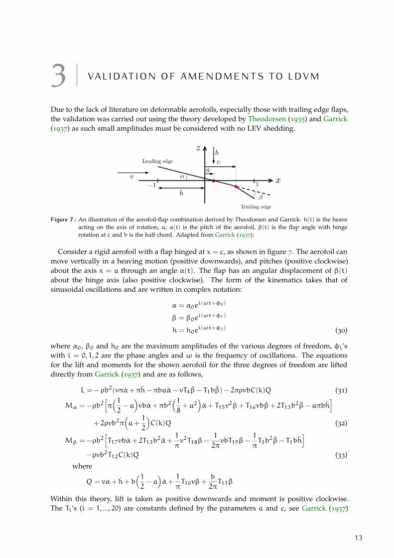
Due to the lack of literature on deformable aerofoils, especially those with trailing edge flaps,the validation was carried out using the theory developed by Theodorsen (1935) and Garrick(1937) as such small amplitudes must be considered with no LEV shedding.

Figure 7.: An illustration of the aerofoil-flap combination derived by Theodorsen and Garrick: h(t) is the heaveacting on the axis of rotation, a; α(t) is the pitch of the aerofoil, β(t) is the flap angle with hingerotation at c and b is the half chord. Adapted from Garrick (1937).

Consider a rigid aerofoil with a flap hinged at x = c, as shown in figure 7. The aerofoil canmove vertically in a heaving motion (positive downwards), and pitches (positive clockwise)about the axis x = a through an angle α(t). The flap has an angular displacement of β(t)about the hinge axis (also positive clockwise). The form of the kinematics takes that ofsinusoidal oscillations and are written in complex notation:

α = α0ei(ωt+φ0)

β = β0ei(ωt+φ1)

h = h0ei(ωt+φ2) (30)

where α0, β0 and h0 are the maximum amplitudes of the various degrees of freedom, φi’swith i = 0, 1, 2 are the phase angles and ω is the frequency of oscillations. The equationsfor the lift and moments for the shown aerofoil for the three degrees of freedom are lifteddirectly from Garrick (1937) and are as follows,

L =− ρb2(vπα+ πh− πbaα− vT4β− T1bβ) − 2πρvbC(k)Q (31)

Mα = −ρb2[π(12− a)vbα+ πb2

(18+ a2

)α+ T15v

2β+ T16vbβ+ 2T13b2β− aπbh

]+ 2ρvb2π

(a+

1

2

)C(k)Q (32)

Mβ = −ρb2[T17vbα+ 2T13b

2α+1

πv2T18β−

1

2πvbT19β−

1

πT3b

2β− T1bh]

−ρvb2T12C(k)Q (33)

where

Q = vα+ h+ b(12− a)α+

1

πT10vβ+

b

2πT11β

Within this theory, lift is taken as positive downwards and moment is positive clockwise.The Ti’s (i = 1, ..., 20) are constants defined by the parameters a and c, see Garrick (1937)

13

14 validation of amendments to ldvm

for their definition. The final unknown, C(k) is known as Theodorsen’s function defined asC(k) = F(k) + iG(k) and can be rewritten using Hankel functions of the second kind.

Comparing the above theory to the expressions used within LDVM, the equation set 30

reduces to the following:

α = α0ei(ωt+φ)

β = β0ei(ωt+ψ)

h =h0cei(ωt) (34)

where the phase angles are the lags for the degrees of freedom with respect to heave. Usingequations 34 and the expressions for lift and moments, a new function is defined within theUNSflow package (which also incorporates LDVM) to calculate the aerodynamic coefficientssuch that they can be compared with the output from LDVM. To do this, L, Mα, Mβ areseparated into three separate terms depicting the contributions due to pitch, heave and theflap:

Lh = −ρb2πh− 2πρUbC(k)h (35)

Lα = −ρb2(Uπα− πbaα) − 2πρUbC(k)(uα+ b

(12− a)α)

(36)

Lβ = −ρb2(−UT4β− T1bβ) − 2πρUbC(k)( 1πT10Uβ+

b

2πT11β

)(37)

Mα,h = −ρb2(−aπbh) + 2πρUb2(a+

1

2

)C(k)h (38)

Mα,α = −ρb2(π(12− a)Ubα+ πb2

(18+ a2

)α)+ 2πρUb2

(a+

1

2

)C(k)

(Uα+ b

(12− a)α)

(39)

Mα,β = −ρb2(T15U2β+ T16Ubβ+ 2T13b

2β) + 2πρUb2(a+

1

2

)C(k)

( 1πT10Uβ+

b

2πT11β

)(40)

Mβ,h = −ρb2(−T1bh) − ρUb2T12C(k)h (41)

Mβ,α = −ρb2(T17Ubα+ 2T13b

2α)− ρUb2

(uα+ b

(12− a)α)

(42)

Mβ,β = −ρb2(1

πU2T18β−

1

2πUbT19β−

1

πT3b

2β) − ρUb2( 1πT10Uβ+

b

2πT11β

). (43)

where v has been replaced with U to follow the notation in LDVM. To continue with the anal-ysis, the above equations are nondimensionalised by 0.5ρU2c for the lift terms and 0.5ρU2c2

for the moments. In the case of Lh,Mα,h andMβ,h, the amplitude taken in by LDVM is h0/c,thus this term is merely nondimensionalised by 0.5ρU2 and 0.5ρU2c. As the expressions 35 -43 contain the half chord, b, the c within the nondimensionalisation is replaced with the halfchord since b = 0.5c. To summarise,

Cl,h =−2LhρU2

, Cmα,h =Mα,h

ρU2b, Cmβ,h =

Mβ,h

ρU2b(44)

Cl,α =−LαρU2b

, Cmα,α =Mα,α

2ρU2b2, Cmβ,α =

Mβ,α

2ρU2b2(45)

Cl,β =−LβρU2b

, Cmα,β =Mα,β

2ρU2b2, Cmβ,β =

Mβ,β

2ρU2b2. (46)

The lift is taken to be negative due to it being defined as positive downwards in Theodorsen’stheory while in LDVM, lift is positive upwards. The final nondimensionalised expressions

validation of amendments to ldvm 15

were derived using symbolic computation within Python (see appendix C for Python script).In addition to this, a steady state contribution to the lift is also considered, Cl,ss = 2π(αmean−α0) where αmean is the mean angle of attack of the chordline and α0 is the zero-lift angle ofattack.

To validate the code, several case studies were conducted using LDVM (with LESPcrit =21, such that LEV shedding is switched off) and Theodorsen: the results were then com-pared. The imaginary form (sinusoid) of equation 34 is selected for the comparison and theparameters within are summarised in the table below:

Table 1.: Test cases for the validation of deformable amendments to LDVM.

Cases α0 () h0/c β0 () ω (rads−1) ψ () φ () xb/c

A 7.5 0.0 0.0 7.86 0.0 0.0 1.0B 0.0 0.1 0.0 7.86 0.0 0.0 1.0C 10.0 0.1 0.0 7.86 0.0 0.0 1.0D 0.0 0.0 2.5 7.86 0.0 0.0 0.5E 7.5 0.1 5.0 7.86 0.0 0.0 0.5

The pivot location where pitch and heave were applied was held fixed throughout atx = 0.2c (i.e. at 20% of the chord length). Initially, the degrees of freedom, pitch, heave andthe flap, were investigated independently and then combinations of them were considered(pitch and heave as well as all three together). For the cases were only pitch and heave wereconsidered, there is no hinge moment and so this comparison is omitted. Figures 8, 9 and 10

show the results for pitch, heave and pitch and heave, respectively.

Figure 8.: Comparison of the results for LDVM and Theodorsen for pitch only (Case A listed in Table 1).


Figure 9.: Comparison of the lift and moment coefficients for LDVM and Theodorsen for heave only (Case Blisted in Table 1).

Figure 10.: Comparison of the lift and moment coefficients for LDVM and Theodorsen for pitch and heave (CaseC listed in Table 1).

In all three cases, LDVM produces results that very closely match those derived usingTheodorsen’s theory. When considering pitch and heave separately, the results for heavecompare more favourably than those for pitch. That is to say the comparison between LDVM


Figure 11.: Comparison of the lift and moment coefficients for LDVM and Theodorsen for the flap only (Case Dlisted in Table 1).

and Theodorsen for heave is much closer than the same comparison for pitch alone (in thecase for lift coefficient).

The comparison for the pitching moment in figure 8 shows that LDVM correctly predictsthe shape of the coefficient with minor differences in the magnitude - it peaks (and troughs)at marginally larger values of Cmα. Figure 10 illustrates the effect of combined pitch andheaving motions (where no phase difference has been applied, the motions are in phase withone another). Again, the results agree well with the theory. If a non-zero phase is used, theresults deviate more substantially with the same values of α0 and h0/c (the values chosen inthe φ = 0 case) - the shape remains the same but the magnitude of the curve increases andbecomes much larger than that predicted by Theodorsen. However, using a non-zero phaseand decreasing the value of the amplitudes of the motions causes an agreement betweenLDVM and Theodorsen. In Ramesh et al. (2014), a more comprehensive comparison betweenLDVM and experimental and numerical results is carried out for much larger values of theamplitudes, phase values and with LEV shedding.


Figure 12.: Comparison of the lift and moment coefficients for LDVM and Theodorsen for pitch, heave and theflap (Case E listed in Table 1).

The validation for the addition of the flap was carried out in two stages: flap only and thenwith all three degrees of freedom combined. Figure 11 gives the comparison of the flap onlycase. Briefly comparing this to the other, individual degrees of freedom, the lift and momentcoefficients for the flap are smaller, by a factor of ten, compared with pitch and heave. Thisindicates that motions from the flap will contribute in small manner to the overall motion ofthe aerofoil. The main reason behind using this case independently is to validate the hingemoment calculation which was added to LDVM. The lower image of figure 11 shows howwell the code compares to Theodorsen’s theory. The curves, once again, have a similar shapealthough there are much larger discrepancies than the comparison for lift and pitching mo-ment coefficients. This may indicate that the code performs poorly at recreating the hingemoment for the flap. However, when considering the values of Cmβ, one can see that magni-tude in error will be very small when the other degrees of freedom are added to the analysis.

To further this hypothesis, the validation continued by adding in pitch and heave to thekinematics (Case E in Table 1). The results for the combined degrees of freedom are shownin figure 12. In this case, where no phase differences are applied (ψ and φ are zero), LDVM


agrees fairly well with Theodorsen. The hinge moment coefficient agrees much better thanthat shown in figure 11 which seems to support that the contributions of pitch and heave aremuch larger than those from the flap. The lift coefficient decreases due to the addition of theflap while the pitching moment increases in magnitude - when comparing the results withand without the flap. With the other degrees of freedom, the hinge moment also increases.

With the addition of another degree of freedom, the number of parameters that can bechanged increases by three; β0, ψ and xb. A comment can be made about the effect of eachof these. If β0 is increased, the comparison worsens due to the small amplitude approx-imation inherent within Theodorsen’s theory as long as β0 < 10 (when the flap is onlyconsidered) then the validation holds. The location of the hinge is also vital to the compari-son: if the hinge is pushed further along the chord towards the trailing edge, LDVM deviatesfrom Theodorsen. However, the values for Cmβ becomes two orders of magnitude smallerthat the lift and pitching moment coefficients. As the location of xb is moved closer to theleading edge, the hinge plays a more important role and the subsequent force coefficientsincrease in magnitude and compare favourably to Theodorsen’s predictions. Including thevariation in phase, a similar trend is seen to that in the pitch and heave case, if the samevalues of the amplitudes are kept for α0, h0/c and β0, the results look vastly different. Thisis, again, due to the small amplitude assumption and if the amplitudes for the kinematicsare reduced the validation holds.

This validation is the first step to ensuring the amendments to LDVM hold true as Theodorsenonly encompasses small variations and no LEV shedding. To ensure that the results willhold true outwith the aforementioned regime, then subsequent validations should be madeexperimentally and numerically. As it was only the aerodynamics validated here (since thekinematics were completely prescribed), a structural model should be devised and added tothe LDVM package. This will allow for a complete validation of the model using flutter anal-ysis (which is by far more documented for a trailing edge flap) to be carried out. However, asan initial validation, the aerodynamics of the aerofoil appear to be correct and so the projectwill proceed by investigating how a trailing edge flap affects the propulsive efficiency.

4 I N V E S T I G AT I O N O F P R O P U L S I O NE F F I C I E N C Y

The main aim of the project is to determine the effect flexibility has on the overall propulsionefficiency. The study is performed in two main steps: 1) conducting numerical analysis ona rigid aerofoil (NACA 0012) to recreate the in Anderson et al. (1998) and 2) the aerofoil ismodified to include a trailing edge flap, using this prescribed structure and the kinematicsof the most efficient cases reported by Anderson et al., a series of simulations are carried outto see if the flap enhances or diminishes the propulsive efficiency.

4.1 rigid aerofoils: recreation of anderson et al.

Figure 13.: An illustration of the rigid aerofoil and the various motions being applied: θ(t) is pitch and h(t) isheave, both of which are applied at the point O in the diagram (i.e. O is the axis of rotation as wellas where heave is applied). Taken from Anderson et al. (1998).

Anderson et al. (1998) considered a high-aspect-ratio aerofoil of chord length c (see figure13), moving at a constant forward speed U undergoing the following harmonic pitching, θ(t),and heaving, h(t), motions:

h(t) =h0c

sin(ωt) (47)

θ(t) = θ0 sin(ωt+ψ) (48)

where h0 and θ0 are the amplitudes of the motions; ω is the frequency and φ is the phasedifference between pitch and heave. Firstly, the pitch is already defined as α within thisreport and LDVM’s literature, hence in future, this notation will be used instead of θ(t) (i.eequation 48 becomes α(t) = α0 sin(ωt + ψ)). The aerofoil undergoes time varying forcesX(t), Y(t) in the forward, x, and transverse, y (in LDVM this is the z direction), directionsrespectively as well as a torgue Q(t) about the pitch axis O (which is located at a third of the

21

22 rigid aerofoils: recreation of anderson et al.

chord length). The period of oscillation is given by T, hence the time-averaged thrust forceas well as the average input power per cycle can be defined as:

F =1

T

∫T0

X(t)dt, (49)

P =1

T

( ∫T0

Y(t)dh

dtdt+

∫T0

Q(t)dα

dtdt

). (50)

These equations are nondimensionalised into their respective coefficients,

CT =F

1/2ρS0U2, (51)

CP =P

1/2ρS0U3(52)

where ρ is the fluid density and S0 is the area of one side of the aerofoil such that, S0 = cs.The propulsive efficiency is subsequently defined as η = CT/CP. Anderson et al. conducttheir research using a nondimensional parameter known as Strouhal number (i.e. Strouhalnumber is chosen and the frequency ω is determined through this):

St =fA

U(53)

where f = ω/(2π) is the frequency in Hz and A is the characteristic width of the generatedjet flow.

Table 2.: Kinematics for the numerical and experimental comparison presented in Anderson et al. (1998)

Kinematics α0 () h0/c ψ ()

Case 1 5 0.75 90

Case 2 15 0.25 90

Case 3 15 0.75 90

Case 4 15 0.75 75

To recreate the results documented by the authors (those shown in figures 6 through 9 ofthe paper), the background theory summarised above must be redefined to follow the struc-ture of LDVM. LDVM reads in a reduced frequency value, k, transforms this into ω anduses this value within the kinematics for pitch and heave whereas Anderson et al. use St tocalculate the frequency. Hence within the scripts used to regenerate the documented results,St is specified and used to determine the usual parameters ω and k which are subsequentlyused to calculate the period, T and the time step dt. Note, the pitch is positive clockwise andheave is positive downwards within Anderson et al. (1998) while the pitch is defined in thesame way, heave is positive upwards in LDVM which has implications for the value of dh/dtin equation 50 - h(t) will be negative in this case. The same is also true for X(t), this forcewill be negative due to the direction of the velocity: it is opposite to that defined in LDVM.

As LDVM outputs the aerodynamic coefficients of aerofoil, they are used directly to calcu-late the thrust and power coefficients,

CT =1

T

∫T0

−Cddt (54)

CP =1

T

( ∫T0

Cl

(−dh

dt

)dt+

∫T0

Cmαdα

dtdt

)(55)

rigid aerofoils: recreation of anderson et al. 23

Experimental

Numerical

LDVM

Figure 14.: Four subplots depicting the recreated results. Top left: LESP vs t/T ; Top right: thrust coefficient as afunction of St; Bottom left: power coefficient as a function of St; Bottom right: efficiency as a functionof St, using Case 1 kinematics in Table 2.

where the force definitions have been replaced by the corresponding definitions in LDVM.The integrations involved are carried out using a numerical integration technique, namelythe trapezoidal method and are performed within the user input script (see appendix Bfor example code for the recreations). The propulsive efficiency is then determined usingη = CT/CP as before.

Anderson et al. report that LEV shedding hinders the thrust generation and overall effi-ciency of the aerofoil and advises that weak or no LEV shedding would be optimal for theefficiency. This aspect was investigated by initially turning off LEV shedding and recreat-ing the above results then choosing a critical LESP value the simulations were run again toobtain figures 14 to 17. A critical value of LESPcrit = 0.25 was chosen as it produced thesmallest error between the results: varying values of LESP were selected and used within ascript, the discrepancies between the numerical/experimental and the results from LDVMwere compared and the LESP that gave the minimal error was chosen to recreate the results.

Figures 14 through 17 show the recreated results using the LDVM. The numerical andexperimental results used in the comparison are taken from the aforementioned paper via aplot digitiser. Figure 14 shows a major discrepancy in the thrust coefficient between LDVMand the experimental results for St > 0.23, while LDVM matches better to the numericalresults. For the power coefficient, the results match fairly closely for low Strouhal numbersand deviate for St > 0.35. Looking at the efficiency for these kinematics, it is clear to see thatabove a certain Strouhal number, St > 0.20 the results become more comparable. Hence, forthe propulsive efficiency, LDVM performs well for the large frequency range when comparedwith the numerical method used by Anderson et al..


Experimental

Numerical

LDVM


Similarly, for figure 15, the thrust and power coefficients follow the same general trendbetween the three documented results (experimental, numerical and LDVM) can be seenhowever, these deviate for large Strouhal numbers (St > 0.3). The propulsive efficiencycontains a minor anomaly at St = 0, a peak point occurs for η. The possible reason behindthis is that LDVM performs poorly for very low frequencies and subsequently, the resultobtained for these such values should be considered an incorrect portrayal of the true trendof the efficiency. Secondly, the results presented by Anderson et al. do not start at such smallvalues of Strouhal number (close to zero), hence a comparison cannot truly be made betweenthe three. For the propulsive efficiency, an increase can be seen before η reaches a peak value,and then it gradually decreases within increasing St. However, LDVM has a much higherpeak value and decreases more rapidly when compared to the experimental and numericalresults.

Figures 16 and 17 are vastly different to the two previous cases. To explain this, for casesone and two, the numerical and experimental results agree fairly well; with LDVM alsoagreeing well with the experimental results, however for cases three and four, this isn’t thecase. The numerical and experimental results reported by Anderson et al. do agree well withone another, but LDVM deviates substantially when compared. These differences can largelybe attributed to the thrust coefficient generated in LDVM as the values obtained are smallerthan the experimental and numerical counterparts. Again, the peak anomaly in η can beseen for cases three and four.

rigid aerofoils: recreation of anderson et al. 25


Experimental

Numerical

LDVM


Anderson et al. concludes that the values of St that produce optimal thrust (hence effi-ciency) are between 0.25 and 0.4, thus using this range and the experimental results (casesgiven in Table 2), the Strouhal numbers associated with the highest propulsive efficiency were


a)

b)

c)

d)

Figure 18.: Vortex wakes and LEV shedding visualisation for certain kinematic parameters: a) Case 1: h0/c =

0.75, α0 = 5, ψ = 90 and St = 0.283 b) Case 2: h0/c = 0.25, α0 = 15, ψ = 90 and St = 0.254 c)Case 3: h0/c = 0.75, α0 = 15, ψ = 90 and St = 0.270 d) Case 4: h0/c = 0.75, α0 = 15, ψ = 75

and St = 0.355

chosen and used to visualise the strength of the vortex wakes. A summary of the Strouhalnumbers and efficiencies is given in Table 3. Figure 18 shows the vortex wake as well as theLEV shedding (if any) generated by the pitching and heaving aerofoil.

Table 3.: Propulsive efficiency comparison between LDVM and experimental results for select Strouhal numbers.

Kinematics St ηexp ηLDVM

Case 1 0.283 0.2048 0.2698Case 2 0.254 0.6242 0.4831Case 3 0.27 0.7715 0.5683Case 4 0.355 0.8552 0.395

In each of the subplots of figure 18, a distinct vortex wake is shed from the trailing edge ofthe aerofoil wherein the vortices alternate in strength, this is particularly noticeable in sub-plots (a), (b) and (d). The wake within (c) has a less well defined structure than the othersbut still shows similar alternation. In all but (b), vortices are shed from the leading edge. Themajority of which are opposite in sign as those attached at the trailing edge. Considering themagnitude of these vortex strengths, the TEVs are stronger than LEVs in (a) and (b) whilein (c) and (d) the LEVs are marginally stronger or comparable to the TEVs. Table 3 alsodocuments the propulsive efficiency. Comparing these results to one another, baring case

deformable aerofoils: trailing edge flap 27

one, LDVM under estimates the efficiency of the aerofoil. Most notably, the efficiency forcase four results in a drastically smaller efficiency, this can be attributed to the strength ofthe LEV as well how they interact with the TEVs - Anderson et al. (1998) concludes throughflow visualisation and subsequent analysis that the position of LEVs are highly dependenton the phase ψ. For case 4, the position of LEVs are predicted to be at 18% of the chord, itseems that LEVs not far along the chord have a significant impact on the thrust productiondue to their positioning and overall strength.

Cases one through three better estimate the efficiency of the aerofoil. Possible reasons forthis are the strength of the vortices (LEV strength is smaller than TEV) as well as the positionof the generated LEVs which are further along the aerofoil chord (roughly 50% accordingto Anderson et al. (1998)). Figures 18(a) and 18(b) show weak LEV shedding. Figure 18(b)shows the features of the flow for low heave amplitudes and its effect on LEV generation. Ash0/c = 0.25, heave motions are small in comparison to the pitching motions, no LEVs areshed from the aerofoil.

To summarise, the analysis presented by Anderson et al. seems to hold true for LDVM:weak or no LEV shedding produces the most optimal cases (i.e. cases on to three) and LEVshave significant impact on the thrust and subsequently the efficiency generated (i.e case 3).In the next section, the results obtained here will be used to investigate the effect of addingan additional degree of freedom (a flap) will have on the efficiency. The rigid cases resultsrecreated in LDVM will be used as a comparison.

4.2 deformable aerofoils: trailing edge flap

The latter half of the project was dedicated to investigating the effect of a trailing edge flapon the propulsive efficiency of the aerofoil. The study was again conducted on a NACA 0012

and used the kinematics of case two and three discussed in the previous section (see Table 2).In addition to the kinematics for pitch and heave, the mathematical formulation of the flapmust also be defined:

β = β0 sin(ωt+φ) (56)

where β0 is the amplitude of the flap deflection; ω is the frequency and φ is the phasedifference between heave and the flap. Due to the flap, the aerofoil has an additional momentapplied to it, the hinge moment, which must be accounted for with regards to the inputpower coefficient. Thus, the following amendment is made to CP:

CP =1

T

( ∫T0

Cl

(−dh

dt

)dt+

∫T0

Cmαdα

dtdt+

∫T0

Cmβdβ

dtdt

). (57)

The expression for the thrust coefficient is as before (see equation 55).

With these definitions, the investigation proceeded by looking at the effect β0, xb and φ hason the propulsive efficiency, η. Initially, the location of the hinge, xb was varied from closeto the trailing edge back towards the pivot location where pitch and heave are applied (i.e.the hinge was moved from the trailing edge to the leading edge). Three values of xb/c werechosen: 0.5, 0.7 and 0.9 and the remainder of the flap parameters were kept fixed (β0 = 10,φ = 0). As anticipated, if the hinge location is pushed towards the leading edge, the flap

28 deformable aerofoils: trailing edge flap

30 6 9 12 15 20(degrees)

30 6 9 12 15 20(degrees)

a) b)

Figure 19.: Effect that varying φ and β0 has on the propulsive efficiency for: St = 0.254, α0 = 15, h0/c = 0.25,ψ = 90 and xb = 0.5. a) No LEV shedding b) With LEV shedding, LESPcrit = 0.18.

plays a more dominant role in thrust and power generation, thus the propulsive efficiency ishigher for aerofoils with xb close to the pivot point. The results are summarised in Table 4.

Table 4.: Effect of hinge location on propulsive efficiency.

Kinematics β0 () φ () xb/c ηLDVM ηLEV

Case 2 10 0 0.9 0.469 0.462710 0 0.7 0.4903 0.465110 0 0.5 0.538 0.4912

Case 3 10 0 0.9 0.662 0.562210 0 0.7 0.6904 0.571510 0 0.5 0.7213 0.5942

ηLDVM documents the efficiency produced using no LEV shedding, if LESPcrit is selectedthat LEV shedding is induced, the efficiency (ηLDVM) still increases with decreasing xb/c,however the attained value of ηLEV is smaller (in comparison to the same case with no LEVs).

Given that xb/c = 0.5 produces the highest ηLDVM, this value is chosen to investigate theeffect of varying β0 and φ. To visualise the effect of changing both of these parameters, ascript was set up to run over five select values of φ (0 to 180 in steps of 45) for β0 ∈ [0, 15].The script (shown in the appendix) was run for the kinematics in case two and case three(Table 2) with the Strouhal numbers listed in table 3, with and without LEV shedding, toshow the effect changing these parameters had on the propulsive efficiency.

Figure 19 shows the results of this variation for case 2. As the value of β0 is increased,the efficiency also increases. When comparing this observation for with and without LEVshedding, this holds true, in general, over the chosen range of β0, however there are certainvalues that produce lower efficiency in the LEV shedding case. One clear difference wheninducing LEV shedding is that the curves are no longer smooth for the different values of φ,this is particularly noticeable for φ = 0, 180. This, in addition to the results in table 4, im-plies that LEV shedding may not aid the propulsive efficiency and in some instances hindersit. For no LEV shedding, the variation of φ initially increases the efficiency until φ = 90

for values above this, it decreases. The same is true when considering LEV shedding. Forthe case with LEV shedding, another interesting phenomena occurs, the curve for φ = 0


a) b)

30 6 9 12 15 20(degrees)

30 6 9 12 15 20(degrees)

Figure 20.: Effect that varying φ and β0 has on the propulsive efficiency for: St = 0.270, α0 = 15, h0/c = 0.75,ψ = 90 and xb = 0.5. a) No LEV shedding b) With LEV shedding, LESPcrit = 0.25.

becomes less efficient compared to the φ = 180.

A similar analysis is conducted using figure 20. For the no LEV shedding case, the sameconclusions can be drawn for increasing β0, however for varying φ, the maximum is reachedat φ = 45, when values above this are chosen, the efficiency decreases. For values ofφ > 135, when increasing β0, the efficiency decreases. When taking LEV shedding intoaccount, the conclusion for varying φ returns to that discussed in figure 19’s analysis. Thesame jaggedness is also seen in the LEV case.

In addition to the above analysis, a visualisation of the vortex wake for a variety of param-eters was performed. Figure 21 shows the flow variation for case two with varying phaseand hinge location of the flap: a) through c) indicate the effects changing hinge location hason the vortex wake and d) through g) show how phase affects the flow. In comparison, thechanges due to hinge location cause marginally stronger and more abundant LEVs to be shedwhile the overall trend of the trailing edge wake is the same for each hinge location. Whenvarying the phase, the LEVs initially increase in strength (and are different in sign to thosein the a) to c)) until φ = 45 and they fall off in strength and abundance above this value. Inaddition to this difference, the trailing edge wake has a series of alternating vortices whichspread out the further from the trailing edge they travel.

For the other case (case three), the flow was also visualised and the differences noted. Tobegin with, due to the larger amplitude in heave, the vortices shed are densely populatedand larger in strength. Figure 22 is split in the same manner as the previous flow visuali-sation: a) to c) vary hinge location and d) to g) vary phase. All subplots have alternatingvortices within their wakes. The variation in hinge location doesn’t change the overall flowfeatures aside from arranging vortices into a more dense clump - initially, the wake is morespread out. The leading edge produces a variation in sign for the LEVs: a) and c) are positivewhile b) has negative LEVs. For the cases were phase is varied, there are almost no LEVsshed except in d) and f) where the phase is an integer value of 45. The phase also causesthe strength of the vortices in the wake to change. As φ increases to 90, the vortex strengthincreases (the red and blue become more deep in colour) while above 90, the strength fallsoff for both (it is more noticeable for positive vortices - the red becomes pale). In addition to


the varying strength, the pockets of vorticity become more spread out with increasing phase.

The final comparison to be made is that of the flow visualisation for the rigid and flappingaerofoil. Figure 18b) corresponds to the rigid case for figure 21 while figure 18c) matcheswith figure 22. For the former of these, the flap introduces positive strength vortices withthe overall profile being largely the same. The propulsive efficiency, in this instance, may besmaller or larger for the flap case than the rigid one depending on the chosen parameters.For the latter comparison, the strength of the LEVs is substantially smaller when consideringa flap and the same conclusion can be drawn about the propulsive efficiency.

Table 5.: Propulsive efficiency for flows shown in figures 21 and 22.

Kinematics β0 () φ () xb/c ηLEV

Case 2 10 0 0.9 0.462710 0 0.7 0.465110 0 0.5 0.491210 45 0.5 0.536710 90 0.5 0.58910 135 0.5 0.545610 180 0.5 0.5041

Case 3 10 0 0.9 0.562210 0 0.7 0.571510 0 0.5 0.594210 45 0.5 0.634810 90 0.5 0.651110 135 0.5 0.608410 180 0.5 0.5544

The propulsive efficiencies for the rigid cases (case two and three) are η = 0.4831, 0.5683,respectively. Table 5 summarises the attained efficiency for the flap cases considered. Assuch, it is clear to see that the flap can either enhance or diminish the overall propulsionexperienced by the aerofoil depending on the parameters chosen.


a)

b)

c)

d)

e)

f)

g)

Figure 21.: Effect that varying φ and xb/c has on flow features for: St = 0.254, α0 = 15, β0 = 10, h0/c = 0.25with LESPcrit = 0.18. a) xb/c = 0.9 and φ = 0 b) xb/c = 0.7 and φ = 0 c) xb/c = 0.5 and φ = 0

d) xb/c = 0.5 and φ = 45 e) xb/c = 0.5 and φ = 90 f) xb/c = 0.5 and φ = 135 g) xb/c = 0.5 andφ = 180.


a)

b)

c)

d)

e)

f)

g)

Figure 22.: Effect that varying φ and xb/c has on flow features for: St = 0.270, α0 = 15, β0 = 10, h0/c = 0.75with LESPcrit = 0.25. a) xb/c = 0.9 and φ = 0 b) xb/c = 0.7 and φ = 0 c) xb/c = 0.5 and φ = 0

d) xb/c = 0.5 and φ = 45 e) xb/c = 0.5 and φ = 90 f) xb/c = 0.5 and φ = 135 g) xb/c = 0.5 andφ = 180.

5 D I S C U S S I O N

Amendments to the LDVM algorithm were carried out based on theory outlined in Katz &Plotkin (2001) and accounted for flexible aerofoils (flat plate with trailing edge flap) under-going oscillatory motions in pitch and heave. Through these amendments, flexibility wasevaluated in terms of its effectiveness to promote optimal propulsion. The initial stages ofthis work, largely, dealt with rederiving key equations and reformulating the mathematicalmodel to account for time-varying camber. The mathematical framework follows similarwork performed by Katz & Weihs and focuses on a simple deformable camber structure.

Following this, validations were carried out to determine how well these amendmentsrecreated the physical system, numerically. However, a lack of literature exists for the chosenstructure of the aerofoil and limited validations were performed. A comparison betweentheory derived by Theodorsen (and continued by Garrick) and the forces and moments cal-culated using LDVM were made. It was found that they agreed fairly well with one another(within reasonable error bounds). Initially, the three degrees of freedom: pitch, heave andflap were validated independently of one another and then with various combinations. Inthe case of pitch and heave, these results were already validated by Ramesh et al., althoughsome validations for this were shown for completeness. The flap only case raised severalconclusions, namely, the contribution due to flap is considerably smaller than the other de-grees of freedom and the comparison had a larger error (when compared with the pitch andheave only cases). The error between LDVM and theory can be neglected to a certain degreedue to magnitude of the flap contribution. When considering all three motions together, thecomparison is favourable and it can be stated that LDVM calculates the forces and momentsfairly well. As previously mentioned, further validations should be conducted, numericallyand experimentally, for a flat plate with trailing edge flap to determine if LDVM performswell for large amplitude motions and LEV shedding as the theory chosen, fundamentally,fails when these are considered.

The main investigation of the project involved recreating results presented by Andersonet al. and extending the rigid aerofoil into the flexible regime. For the recreation stage, LDVMwas used to determine the propulsive efficiency for a rigid aerofoil undergoing pitching andheaving motions. The theory outlined by Anderson et al. was transferred into the notationused by LDVM. Four cases were recreated using LDVM (see Table 2). The first part of therecreation dealt with determining the propulsive efficiency as a function of Strouhal numberand how well LDVM compared with the experimental and numerical results presented in theaforementioned paper. It was shown that for certain parameter sets, LDVM’s results moreclosely resembled their experimental and numerical counterparts: with the best recreationbeing made for case two (α0 = 15degree, h0/c = 0.25 and ψ = 90). Further to this, LDVMalso drew the conclusion that optimal efficiency can be achieved when weak or no LEVsare shed. However, when considering the most efficient experimental cases, the efficiencyestimated by LDVM performs poorly: the efficiency is underestimated in three of the fourcases, with the worst performance obtained from case four - a loss of efficiency by 46% (seeTable 3). The final section of the recreation dealt with the visualisation of the vortex wakeand the key features within it. The wake consisted of vortices of alternating vortex strength

33

34 discussion

and with weak or no LEVs being shed at all. In the case with weak heaving amplitude, nopositive strength vortices were seen.

The effect of flexibility was determined for two of the four rigid cases examined in therecreation segment of the project. The addition of a trailing edge flap introduced three newparameters that could be varied: β0, xb/c and φ. It was found that moving the location ofthe hinge closer to the pitch axis (or leading edge) increased the contribution the flap made tothe overall thrust and propulsion of the aerofoil. After fixing the hinge location at xb/c = 0.5,the two other parameters were varied to determine their effect. As to be expected, increasingthe flap amplitude also increases the propulsive efficiency but only for specific phase angles.For case two, the propulsive efficiency always increases (even with LEV shedding), the sameis not true for case three: LEV shedding and certain φ cause the efficiency to decrease withincreasing β0. A more concise conclusion can be drawn from the variation of φ, for fixedβ0, the propulsive efficiency will increase until φ = 90 and will then begin to decreaseagain. Thus, the most optimal value of φ is 90. The effect of LEVs was also investigated atthis point and it was determined that the efficiency decreased somewhat when LEVs wereshed. The flow features were visualised: alternating vortices were seen in the wake withcertain cases inducing weak LEV shedding. For the visualised flows, the efficiencies for eachwere recorded and compared with their respective rigid counterparts. For the cases werethe flap was close to the trailing edge, the efficiencies were not improved. With the hinge atxb/c = 0.5, the flap produced substantial contributions such that the propulsive efficiencywas greater than that seen in the rigid case. An improvement of up to 11% was achieved.Hence, for certain kinematics, the addition of deformable camber aids the propulsion of aero-foils: a conclusion also drawn by several other authors (Katz & Weihs, 1978; Prempraneerachet al., 2003; Miao & Ho, 2006; Hoke et al., 2015).

Future work should include a more rigorous study to determine the full parameter spacethat efficiency is enhanced within (as well as any regimes that cause a diminishment). Ex-perimental and numerical studies should be considered to gain further validation evidenceand to determine how well LDVM performs over a wider range of parameters. As onlythe aerodynamics were validated here, it would be worthwhile to couple a structural modeland perform a flutter analysis. The trailing edge flap was an initial stepping stone into theflexible regime, a completely flexible structure should be implemented next (e.g. a flexiblebeam). This would then be used to recreate the results of the rubberised aerofoil discussedin Prempraneerach et al. (2003) with predefined kinematics. Further to this, a structural pro-gram (e.g Abaqus or MBDyn) should be coupled to LDVM to create a model that deforms abody dependent on the aerodynamic forces applied to the structure at certain time steps.

R E F E R E N C E S

Alben, S., Witt, C., Baker, T.V., Anderson, E. & Lauder, G.V. 2012 Dynamics of freelyswimming flexible foils. Physics of Fluids (1994-present) 24 (5), 051901.

Anderson, J.M., Streitlien, K., Barrett, D.S. & Triantafyllou, M.S. 1998 Oscillating foilsof high propulsive efficiency. Journal of Fluid Mechanics 360, 41–72.

Behbahani, S.B., Wang, J. & Tan, X. 2013 A dynamic model for robotic fish with flexible pec-toral fins. In 2013 IEEE/ASME International Conference on Advanced Intelligent Mechatronics,pp. 1552–1557.

Bergami, L. & Gaunaa, M. 2010 Stability investigation of an airfoil section with active flapcontrol. Wind Energy 13 (2-3), 151–166.

Blake, R.W. 2004 Fish functional design and swimming performance. Journal of Fish Biology65 (5), 1193–1222.

Borazjani, I. 2015 Simulations of unsteady aquatic locomotion: from unsteadiness instraight-line swimming to fast-starts. Integrative and comparative biology 55 (4), 740–752.

Breder, C.M. 1926 The locomotion of fishes, , vol. 4. Zoologica (N.Y.).

Chopra, M.G. 1974 Hydromechanics of lunate-tail swimming propulsion. Journal of FluidMechanics 64, 375–392.

Esfahani, J.A., Karbasian, H.R. & Barati, E. 2015 Proposed kinematic model for fish-likeswimming with two pitch motions. Ocean Engineering 104, 319 – 328.

Garrick, I. E. 1937 Propulsion of a flapping and oscillating airfoil. NACA Report 597.

Glauert, H. 1983 The elements of aerofoil and airscrew theory. Cambridge University Press.

Heathcote, S. & Gursul, I. 2007 Flexible flapping airfoil propulsion at low reynolds num-bers. AIAA journal 45 (5), 1066–1079.

Heathcote, S., Wang, Z. & Gursul, I. 2008 Effect of spanwise flexibility on flapping wingpropulsion. Journal of Fluids and Structures 24 (2), 183–199.

Hoke, C.M., Young, J. & Lai, J.C.S. 2015 Effects of time-varying camber deformation onflapping foil propulsion and power extraction. Journal of Fluids and Structures 56, 152–176.

Hover, F.S., Haugsdal, Ø. & Triantafyllou, M.S. 2004 Effect of angle of attack profiles inflapping foil propulsion. Journal of Fluids and Structures 19 (1), 37–47.

Jaworski, J.W. 2012 Thrust and aerodynamic forces from an oscillating leading edge flap.AIAA journal 50 (12), 2928–2931.

Jones, K.D., Castro, B.M., Mahmoud, O., Pollard, S.J., Platzer, M.F., Neef, M.F., Gonet, K.& Hummel, D. 2002 A collaborative numerical and experimental investigation of flapping-wing propulsion. AIAA paper 706.

35

36 References

Karpouzian, G., Spedding, G. & Cheng, H.K. 1990 Lunate-tail swimming propulsion. part2. performance analysis. Journal of Fluid Mechanics 210, 329–351.

Katz, J. & Plotkin, A. 2001 Low-Speed Aerodynamics. Cambridge University Press.

Katz, J. & Weihs, D. 1978 Hydrodynamic propulsion by large amplitude oscillation of anairfoil with chordwise flexibility. Journal of Fluid Mechanics 88 (03), 485–497.

Korsmeyer, K.E., Steffensen, J.F. & Herskin, J. 2002 Energetics of median and pairedfin swimming, body and caudal fin swimming, and gait transition in parrotfish (scarusschlegeli) and triggerfish (rhinecanthus aculeatus). Journal of experimental biology 205 (9),1253–1263.

Krzysiak, A. & Narkiewicz, J. 2006 Aerodynamic loads on airfoil with trailing-edge flappitching with different frequencies. Journal of aircraft 43 (2), 407–418.

Lai, P.S.K., Bose, N. & McGregor, R.C. 1993 Wave propulsion from a fexible-armed, rigid-foil propulsor. Marine technology 30 (1), 30–38.

Lighthill, J. 1960 Note on the swimming of slender fish. Journal of fluid Mechanics 9 (02),305–317.

Lighthill, J. 1975 Mathematical biofluiddynamics, , vol. 17. Siam.

Lighthill, M.J. 1970 Aquatic animal propulsion of high hydromechanical efficiency. Journalof Fluid Mechanics 44 (02), 265–301.

Lindsey, C.C. 1978 1 - form, function, and locomotory habits in fish. In Locomotion (ed. W.S.Hoar & D.J. Randall), Fish Physiology, vol. 7, pp. 1 – 100. Academic Press.

Liu, H. & Kawachi, K. 1999 A numerical study of undulatory swimming. Journal of Compu-tational Physics 155 (2), 223–247.

Martín-Alcántara, A., Fernandez-Feria, R. & Sanmiguel-Rojas, E. 2015 Vortex flowstructures and interactions for the optimum thrust efficiency of a heaving airfoil at differentmean angles of attack. Physics of Fluids (1994-present) 27 (7), 073602.

McCune, J.E. & Tavares, T.S. 1993 Perspective: unsteady wing theory—the kármán/searslegacy. Journal of fluids engineering 115 (4), 548–560.

Miao, J.M. & Ho, M.H. 2006 Effect of flexure on aerodynamic propulsive efficiency of flap-ping flexible airfoil. Journal of Fluids and Structures 22 (3), 401–419.

Michelin, S. & Smith, S.G.L. 2009 Resonance and propulsion performance of a heavingflexible wing. Physics of Fluids (1994-present) 21 (7), 071902.

Moore, M.N.J. 2014 Analytical results on the role of flexibility in flapping propulsion. Journalof Fluid Mechanics 757, 599–612.

Mueller, T.J. 2001 Fixed and Flapping Wing Aerodynamics for Micro Air Vehicle Applications.American Institute of Aeronautics & Astronautics.

Murua, J., Palacios, R. & Peiró, J. 2010 Camber effects in the dynamic aeroelasticity ofcompliant airfoils. Journal of Fluids and Structures 26 (4), 527–543.

Paraz, F., Eloy, C. & Schouveiler, L. 2014 Experimental study of the response of a flexibleplate to a harmonic forcing in a flow. Comptes Rendus Mécanique 342 (9), 532–538.

References 37

Paraz, F., Schouveiler, L. & Eloy, C. 2016 Thrust generation by a heaving flexible foil:Resonance, nonlinearities, and optimality. Physics of Fluids (1994-present) 28 (1), 011903.

Prempraneerach, P., Hover, F.S. & Triantafyllou, M.S. 2003 The effect of chordwise flex-ibility on the thrust and efficiency of a flapping foil. Proceedings Unmanned, UntetheredSubmersible Technology .

Ramesh, K., Gopalarathnam, A., Edwards, J. R, Ol, M.V. & Granlund, K. 2013 An un-steady airfoil theory applied to pitching motions validated against experiment and com-putation. Theoretical and Computational Fluid Dynamics 27 (6), 843–864.

Ramesh, K., Gopalarathnam, A., Granlund, K., Ol, M.V. & Edwards, J.R. 2014 Discrete-vortex method with novel shedding criterion for unsteady aerofoil flows with intermittentleading-edge vortex shedding. Journal of Fluid Mechanics 751, 500–538.

Read, D.A., Hover, F.S. & Triantafyllou, M.S. 2003 Forces on oscillating foils for propulsionand maneuvering. Journal of Fluids and Structures 17 (1), 163–183.

Sfakiotakis, M., Lane, D.M. & Davies, J.B.C. 1999 Review of fish swimming modes foraquatic locomotion. IEEE Journal of Oceanic Engineering 24 (2), 237–252.

Shukla, R.K. & Eldredge, J.D. 2007 An inviscid model for vortex shedding from a deformingbody. Theoretical and Computational Fluid Dynamics 21 (5), 343–368.

Theodorsen, T. 1932 On the theory of wing sections with particular reference to the liftdistribution .

Theodorsen, T. 1933 Theory of wing sections of arbitrary shape .

Theodorsen, T. 1935 General theory of aerodynamic instability and the mechanism of flutter.NACA Report 496.

Triantafyllou, M.S., Triantafyllou, G.S. & Gopalkrishnan, R. 1991 Wake mechanics forthrust generation in oscillating foils. Physics of Fluids A: Fluid Dynamics (1989-1993) 3 (12),2835–2837.

Triantafyllou, M.S., Triantafyllou, G.S. & Yue, D.K.P. 2000 Hydrodynamics of fishlikeswimming. Annual review of fluid mechanics 32 (1), 33–53.

Tuncer, I.H. & Kaya, M. 2005 Optimization of flapping airfoils for maximum thrust andpropulsive efficiency. AIAA journal 43 (11), 2329–2336.

Videler, J.J. 1993 Fish Swimming. Springer Netherlands.

Wagner, H. 1925 Über die entstehung des dynamischen auftriebes von tragflügeln. ZAMM-Journal of Applied Mathematics and Mechanics/Zeitschrift für Angewandte Mathematik undMechanik 5 (1), 17–35.

Wu, T. Y.-T. 1961 Swimming of a waving plate. Journal of Fluid Mechanics 10 (03), 321–344.

Young, J., Lai, J.C.S., Kaya, M. & Tuncer, I.H. 2006 Thrust and efficiency of propulsion byoscillating foils. In Computational Fluid Dynamics 2004, pp. 313–318. Springer.

A U N S F LO W PA C K A G E

The UNSflow package (LDVM) is available as open source software from: github.com/

KiranUofG/UNSflow. Due to the length of the scripts required to run the program, theseare omitted from the appendix and can instead be viewed at the aforementioned website. Asummary of what is carried out within each script is instead listed below.

UNSflow.jl: this is the main file required to run the software package. It pulls in allthe necessary Python packages, functions, solvers and mathematical tools needed bythe user. If packages are missing or further packages are required then the user shouldamend the appropriate call within this module (e.g. if more plot capabilities are needed,export the appropriate function in PyPlot).

types.jl: due to the amount of inputs that define the system, a separate script houses thevariables (with their various types) to make calling further functions more manageable.The system is then easily defined in terms of kinematic defintions, surf definitionsand curfield definitions. In addition to this, within types.jl, the structure of functionswith the parameters needed to run them are also defined. For example, the kinematicsare defined as an amended harmonic function as a mean value plus some additionalcosine or sine function - this is set up within this script such that SinDef(mean_amp,amp, freq, phase) is called instead of the full function. Constraints placed on thesystem such as Kelvin’s condition are also defined here. For the deformable case, newkinematic definitions; a function to calculate all necessary parameters for the flappingaerofoil (TwoDSurfwFlap); new type definitions for Theodorsen (with and without theflap) and a definition for time-varying camber were all added to this module.

calculations.jl: this module contained all the necessary calculations needed for theLDVM solver including those for the: Fourier coefficients, downwash equation, veloc-ity of the vortices, locations of the bound vortices, camber and its derivatives, placingof LEVs and TEVs, how the wake rolls, vortex interactions, induced velocities andthe updating of all the aforementioned quantities. The vast majority of this code wasuntouched, however additional calculations for the downwash and camber (in the de-formable case) were added.

postprocess.jl: the post processing at each time step is conducted using the functionsdefined in this module. This includes the calculation of the aerodynamic force coef-ficients: pitching moment, hinge moment, lift and drag as well as the visualisationof the vortex wake. The new calculations added due to the structure of the aerofoildiscussed in the main text are view_vorts(surf::TwoDSurfwFlap, field::TwoDFlowField)and calc_forces(surf::TwoDSurfwFlap, dt).

solvers.jl: this is the final script used with UNSflow. It contains various numericalalgorithms used for different flow types. The main functions used for this projectare Theodorsen’s calculation for the flapping and oscillating aerofoil and the LDVMalgorithm. LDVM’s structure is discussed in detail in Ramesh et al. (2014).

39

github.com/KiranUofG/UNSflow

github.com/KiranUofG/UNSflow

B U S E R I N P U T S C R I P T S

Listing B.1: Example script used to recreate the results presented in Anderson et al. (1998).

1 workspace()2 include("../../src/UNSflow.jl")3 using UNSflow45 c = 1.6 u_ref = 1.7 h_amp = 0.758 theta_amp = 5*pi/180.9 alpha_max = 5*pi/180.

10 phi = 90.*pi/18011 alpha_mean = 0.12 A = 2*h_amp13 pvt = 1./3.1415 cp = zeros(10)16 ct = zeros(10)17 eta = zeros(10)18 st_le = zeros(10)1920 for j = 1:102122 st = (j-0.99)*0.6/10.23 f = st*u_ref/A24 w = 2*pi*f25 k = w/2.26 T = (2*pi/w)27 ncyc = 1.28 t_tot = ncyc*T29 dt = 0.015*0.2*4/(k*h_amp)3031 nsteps =round(Int,t_tot/dt)+132 range = round(Int,(ncyc-1)*nsteps/ncyc)+1:nsteps3334 hdot = zeros(length(range))35 alphadot = zeros(length(range))3637 hdef = SinDef(0.,h_amp,w,0.)38 alphadef = SinDef(alpha_mean, theta_amp, w, phi)39 udef = ConstDef(1.)40 full_kinem = KinemDef(alphadef, hdef, udef)4142 lespcrit = [0.25;]4344 surf = TwoDSurf(c, u_ref, "FlatPlate", pvt, 70, 35, "Prescribed", full_kinem,

lespcrit)4546 curfield = TwoDFlowField()47

41

42 user input scripts

48 ldvm(surf, curfield, nsteps, dt)4950 data = readdlm("results.dat")51 writedlm("and_test.dat",data)5253 data = readdlm("and_test.dat")5455 tbyT = (data[range,1]-data[range[1]])/T5657 for i = 1:length(range)58 hdot[i] = ForwardDiff.derivative(hdef,data[range[i]])*u_ref59 alphadot[i] = ForwardDiff.derivative(alphadef,data[range[i]])*u_ref/c60 end6162 LESP = data[range,5]63 cl = data[range,6]64 cd = data[range,7]65 cm = data[range,8]6667 ct[j] = (1./T)*trapz(-cd,tbyT)68 cp[j] = (1./T)*(trapz(-cl.*hdot,tbyT)+trapz(cm.*alphadot,tbyT))6970 eta[j] = ct[j]/cp[j]7172 st_le[j] = st7374 global ct75 global cp76 global eta77 global st_le78 global LESP79 global tbyT8081 end8283 data_6anum = readdlm("Fig6aNum.csv")84 data_6aexp = readdlm("Fig6aExp.csv")85 data_6bnum = readdlm("Fig6bNum.csv")86 data_6bexp = readdlm("Fig6bExp.csv")87 data_6cnum = readdlm("Fig6cNum.csv")88 data_6cexp = readdlm("Fig6cExp.csv")8990 using LaTeXStrings91 f = figure("pyplot_subplot_mixed",figsize=(15,5))9293 ax = subplot(221)94 plot(tbyT,LESP,"k-")95 xlabel(L"$t/T$")96 ylabel(L"$LESP$")9798 ax = subplot(222)99 scatter(st_le, ct,color="r",label=L"LDVM",marker="^")

100 scatter(data_6anum[:,1],data_6anum[:,2],color="b",label=L"Numerical",marker="o")101 scatter(data_6aexp[:,1],data_6aexp[:,2],color="g",label=L"Experimental",marker="

x")102 xlabel(L"$St$")103 ylabel(L"$C_T$")

user input scripts 43

104 legend(loc="upper left",fancybox="true")105106 ax = subplot(223)107 scatter(st_le, cp,color="r",marker="^")108 scatter(data_6bnum[:,1],data_6bnum[:,2],color="b",marker="o")109 scatter(data_6bexp[:,1],data_6bexp[:,2],color="g",marker="x")110 xlabel(L"$St$")111 ylabel(L"$C_P$")112113114 ax = subplot(224)115 scatter(st_le, eta,color="r",marker="^")116 scatter(data_6cnum[:,1],data_6cnum[:,2],color="b",marker="o")117 scatter(data_6cexp[:,1],data_6cexp[:,2],color="g",marker="x")118 xlabel(L"$St$")119 ylabel(L"$\eta$")

Listing B.2: Example script used to visualise the flow features for selected kinematic parameters for the rigidaerofoil case.

1 workspace()2 include("../../src/UNSflow.jl")3 using UNSflow45 c = 1.6 u_ref = 1.7 h_amp = 0.758 theta_amp = 5*pi/180.9 alpha_max = 5*pi/180.

10 phi = 90.*pi/18011 alpha_mean = 0.12 A = 2*h_amp13 pvt = 1./3.1415 st = 0.28316 f = st*u_ref/A17 w = 2*pi*f18 k = w/2.19 T = (2*pi/w)20 ncyc = 4.21 t_tot = ncyc*T22 dt = 0.015*0.2*4/(k*h_amp)2324 nsteps =round(Int,t_tot/dt)+125 range = round(Int,(ncyc-1)*nsteps/ncyc)+1:nsteps2627 hdot = zeros(length(range))28 alphadot = zeros(length(range))2930 hdef = SinDef(0.,h_amp,w,0.)31 alphadef = SinDef(alpha_mean, theta_amp, w, phi)32 udef = ConstDef(1.)33 full_kinem = KinemDef(alphadef, hdef, udef)3435 lespcrit = [0.25;]3637 surf = TwoDSurf(c, u_ref, "FlatPlate", pvt, 70, 35, "Prescribed", full_kinem,

lespcrit)


3839 curfield = TwoDFlowField()4041 ldvm(surf, curfield, nsteps, dt)4243 data = readdlm("results.dat")44 writedlm("and_test.dat",data)4546 data = readdlm("and_test.dat")4748 tbyT = (data[range,1]-data[range[1]])/T4950 for i = 1:length(range)51 hdot[i] = ForwardDiff.derivative(hdef,data[range[i]])*u_ref52 alphadot[i] = ForwardDiff.derivative(alphadef,data[range[i]])*u_ref/c53 end5455 LESP = data[range,5]56 cl = data[range,6]57 cd = data[range,7]58 cm = data[range,8]5960 ct = (1./T)*trapz(-cd,tbyT)61 cp = (1./T)*(trapz(-cl.*hdot,tbyT)+trapz(cm.*alphadot,tbyT))6263 eta = ct/cp6465 figure(0)66 view_vorts(surf, curfield)

Listing B.3: Example script used to determine how the propulsive efficiency varies with phase and flap ampli-tude.

1 workspace()2 include("../src/UNSflow.jl")3 using UNSflow45 c = 1.6 u_ref = 1.7 h_amp = 0.258 alpha_amp = 15*pi/180.9 phi = 90.*pi/180

10 A = 2*h_amp11 pvt = 1./3.12 psi = 90*pi/180.13 phi = 0.1415 st = 0.25416 f = st*u_ref/A17 w = 2*pi*f18 k = w/2.19 T = (2*pi/w)20 ncyc = 4.21 t_tot = ncyc*T22 dt = 0.015*0.2*4/(k*h_amp)2324 nsteps =round(Int,t_tot/dt)+125 range = round(Int,(ncyc-1)*nsteps/ncyc)+1:nsteps


2627 hdot = zeros(length(range))28 alphadot = zeros(length(range))29 betadot = zeros(length(range))30 mat = zeros(40,2,5)31 index = 132 for i = 1:53334 phi = (i-1)*pi/4.3536 for j = 1:403738 amp = (j - 1)*15.*pi/(180*40)39 beta_amp = amp4041 hdef = SinDef(0.,h_amp,w,0.)42 alphadef = SinDef(0., alpha_amp, w, psi)43 udef = ConstDef(1.)44 ndef = SinDef(0.,beta_amp,w,phi)45 full_kinem = KinemDefwFlap(alphadef, hdef, udef, ndef)4647 lespcrit = [0.18;]48 x_b = [0.5;]4950 surf = TwoDSurfwFlap(c, u_ref, "FlatPlate", pvt, 70, 35, "Prescribed",

full_kinem, x_b, lespcrit)5152 curfield = TwoDFlowField()5354 ldvm(surf, curfield, nsteps, dt)5556 data = readdlm("results.dat")57 tbyT = (data[range,1]-data[range[1]])/T5859 for i = 1:length(range)60 hdot[i] = ForwardDiff.derivative(hdef,data[range[i]])*u_ref61 alphadot[i] = ForwardDiff.derivative(alphadef,data[range[i]])*u_ref/c62 betadot[i] = ForwardDiff.derivative(ndef,data[range[i]])*u_ref/c63 end6465 LESP = data[range,5]66 cl = data[range,6]67 cd = data[range,7]68 cma = data[range,8]69 cmb = data[range,9]7071 ct = (1./T)*trapz(-cd,tbyT)72 cp = (1./T)*(trapz(-cl.*hdot,tbyT)+trapz(cma.*alphadot,tbyT)+trapz(cmb.*betadot,

tbyT))7374 eta = ct/cp7576 mat[j,:,index] = [amp eta]7778 end79 index = index + 180 end


81 using LaTeXStrings82 figure(1)83 plot(mat[:,1,1],mat[:,2,1],"k-",label=L"\phi=0")84 plot(mat[:,1,2],mat[:,2,2],"b-",label=L"\phi=45")85 plot(mat[:,1,3],mat[:,2,3],"g-",label=L"\phi=90")86 plot(mat[:,1,4],mat[:,2,4],"m-",label=L"\phi=135")87 plot(mat[:,1,5],mat[:,2,5],"r-",label=L"\phi=180")88 legend(loc="upper left",fancybox="true")89 xlabel(L"$\beta_0$")90 ylabel(L"$\eta$")

Listing B.4: Example script used to visualise the changes in flow features with varying hinge location; flapamplitude and phase.

1 workspace()2 include("../src/UNSflow.jl")3 using UNSflow45 c = 1.6 u_ref = 1.7 h_amp = 0.758 alpha_amp = 15*pi/180.9 beta_amp = 10*pi/180.

10 phi = 90.*pi/18011 A = 2*h_amp12 pvt = 1./3.13 psi = 90*pi/180.14 phi = 180*pi/180.1516 st = 0.2717 f = st*u_ref/A18 w = 2*pi*f19 k = w/2.20 T = (2*pi/w)21 ncyc = 4.22 t_tot = ncyc*T23 dt = 0.015*0.2*4/(k*h_amp)2425 nsteps =round(Int,t_tot/dt)+126 range = round(Int,(ncyc-1)*nsteps/ncyc)+1:nsteps2728 hdot = zeros(length(range))29 alphadot = zeros(length(range))30 betadot = zeros(length(range))3132 hdef = SinDef(0.,h_amp,w,0.)33 alphadef = SinDef(0., alpha_amp, w, psi)34 udef = ConstDef(1.)35 ndef = SinDef(0.,beta_amp,w,phi)36 full_kinem = KinemDefwFlap(alphadef, hdef, udef, ndef)3738 lespcrit = [0.25;]39 x_b = [0.5;]4041 surf = TwoDSurfwFlap(c, u_ref, "FlatPlate", pvt, 70, 35, "Prescribed",

full_kinem, x_b, lespcrit)4243 curfield = TwoDFlowField()


4445 ldvm(surf, curfield, nsteps, dt)4647 data = readdlm("results.dat")48 tbyT = (data[range,1]-data[range[1]])/T4950 for i = 1:length(range)51 hdot[i] = ForwardDiff.derivative(hdef,data[range[i]])*u_ref52 alphadot[i] = ForwardDiff.derivative(alphadef,data[range[i]])*u_ref/c53 betadot[i] = ForwardDiff.derivative(ndef,data[range[i]])*u_ref/c54 end5556 LESP = data[range,5]57 cl = data[range,6]58 cd = data[range,7]59 cma = data[range,8]60 cmb = data[range,9]6162 ct = (1./T)*trapz(-cd,tbyT)63 cp = (1./T)*(trapz(-cl.*hdot,tbyT)+trapz(cma.*alphadot,tbyT)+trapz(cmb.*betadot,

tbyT))6465 eta = ct/cp6667 figure(0)68 view_vorts(surf, curfield)

C D E R I VAT I O N S

Listing C.1: Python script used to derive the individual contributions to lift and moment due to the three degreesof freedom (see Section 3).

1 from sympy import *234 var(’h0 alpha0 beta0 w t k C a phi psi c’)5 var(’t1 t2 t3 t4 t5 t6 t7 t8 t9 t10’)6 var(’t11 t12 t13 t14 t15 t16 t17 t18 t19 t20’)78 u, rho, b = var(’u rho b’)9

10 h = -h0*exp(I*w*t)11 alpha = alpha0*exp(I*(w*t+phi))12 beta = beta0*exp(I*(w*t+psi))1314 P_h = -rho*b*b*pi*diff(h,t,2)-2*rho*u*pi*b*C*diff(h,t,1)15 Cl_h = simplify(-2*P_h/(rho*u*u))16 Cl_h = simplify(Cl_h.subs(b*w,u*k))1718 P_alpha = -rho*b*b*(u*pi*diff(alpha,t,1)-pi*b*a*diff(alpha,t,2)) - 2*rho*u*b*C*

pi*(u*alpha+b*(1/2-a)*diff(alpha,t,1))19 Cl_alpha = simplify(-P_alpha/(rho*u*u*b))20 Cl_alpha = simplify(Cl_alpha.subs(b*w,u*k))2122 P_beta = -rho*b*b*(-u*t4*diff(beta,t,1) - t1*b*diff(beta,t,2)) - 2*rho*u*b*C*pi

*(t10*u*beta/pi + (b*t11*diff(beta,t,1)/2)/pi)23 Cl_beta = simplify(-P_beta/(rho*u*u*b))24 Cl_beta = simplify(Cl_beta.subs(b*w,u*k))2526 M_alpha_h = -rho*b*b*(-a*pi*b*diff(h,t,2))+2*rho*u*b*b*pi*(a+1/2)*C*diff(h,t,1)27 Cm_alpha_h = simplify(M_alpha_h/(rho*u*u*b))28 Cm_alpha_h = simplify(Cm_alpha_h.subs(b*w,u*k))2930 M_alpha_alpha = -rho*b*b*(pi*(1/2-a)*u*b*diff(alpha,t,1)+pi*b*b*(1/8+a*a)*diff(

alpha,t,2))+2*rho*u*b*b*pi*(a+1/2)*C*(u*alpha+b*(1-2-a)*diff(alpha,t,1))31 Cm_alpha_alpha = simplify(M_alpha_alpha/(2*rho*u*u*b*b))32 Cm_alpha_alpha = simplify(Cm_alpha_alpha.subs(b*w,u*k))3334 M_alpha_beta = -rho*b*b*(t15*u*u*beta+t16*u*b*diff(beta,t,1)+2*t13*b*b*diff(beta

,t,2)) +2*rho*u*b*b*pi*(a+1/2)*C*(t10*u*beta/pi+(b*t11*diff(beta,t,1)/2)/pi)35 Cm_alpha_beta = simplify(M_alpha_beta/(2*rho*u*u*b*b))36 Cm_alpha_beta = simplify(Cm_alpha_beta.subs(b*w,u*k))3738 M_beta_h = -rho*b*b*(-t1*b*diff(h,t,2))-rho*u*b*b*t12*C*diff(h,t,1)39 Cm_beta_h = simplify(M_beta_h/(rho*u*u*b))40 Cm_beta_h = simplify(Cm_beta_h.subs(b*w,u*k))4142 M_beta_alpha = -rho*b*b*(t17*u*b*diff(alpha,t,1)+2*t13*b*b*diff(alpha,t,2))-rho*

u*b*b*t12*C*(u*alpha+b*(1/2-a)*diff(alpha,t,1))

49

50 derivations

43 Cm_beta_alpha = simplify(M_beta_alpha/(2*rho*u*u*b*b))44 Cm_beta_alpha = simplify(Cm_beta_alpha.subs(b*w,u*k))4546 M_beta_beta = -rho*b*b*(u*u*t18*beta/pi - (u*b*t19*diff(beta,t,1)/2)/pi - t3*b*b

*diff(beta,t,2)/pi) - rho*u*b*b*t12*C*(t10*u*beta/pi + (b*t11*diff(beta,t,1)/2)/pi)

47 Cm_beta_beta = simplify(M_beta_beta/(2*rho*u*u*b*b))48 Cm_beta_beta = simplify(Cm_beta_beta.subs(b*w,u*k))

Documents

2229198m_Merchant_ENG5059P_Thesis_2016