CHAPTER 2MODELING

DISTRIBUTIONS OF DATA

2.2Density Curves and

Normal Distributions

Exploring Quantitative Data

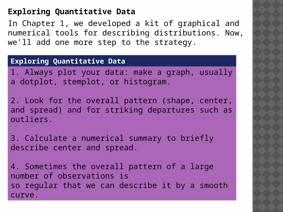
In Chapter 1, we developed a kit of graphical and numerical tools for describing distributions. Now, we’ll add one more step to the strategy.

1. Always plot your data: make a graph, usually a dotplot, stemplot, or histogram.

2. Look for the overall pattern (shape, center, and spread) and for striking departures such as outliers.

3. Calculate a numerical summary to briefly describe center and spread.

4. Sometimes the overall pattern of a large number of observations isso regular that we can describe it by a smooth curve.

Exploring Quantitative Data

A density curve is a curve that*is always on or above the horizontal axis, and*has area exactly 1 underneath it.

A density curve describes the overall pattern of a distribution. The area under the curve and above any interval of values on the horizontal axis is the proportion of all observations that fall in that interval.A symmetric curve balances at its center because the two sides are identical. The mean and median of a symmetric density curve are equal, as in figure (a) below.

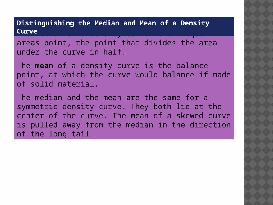
The median of a density curve is the equal-areas point, the point that divides the area under the curve in half.

The mean of a density curve is the balance point, at which the curve would balance if made of solid material.

The median and the mean are the same for a symmetric density curve. They both lie at the center of the curve. The mean of a skewed curve is pulled away from the median in the direction of the long tail.

Distinguishing the Median and Mean of a Density Curve

*A density curve is an idealized description of a distribution of data.

*We distinguish between the mean and standard deviation of the density curve and the mean and standard deviation computed from the actual observations.

*The usual notation for the mean of a density curve is µ (the Greek letter mu). We write the standard deviation of a density curve as σ (the Greek letter sigma).

Normal Distributions

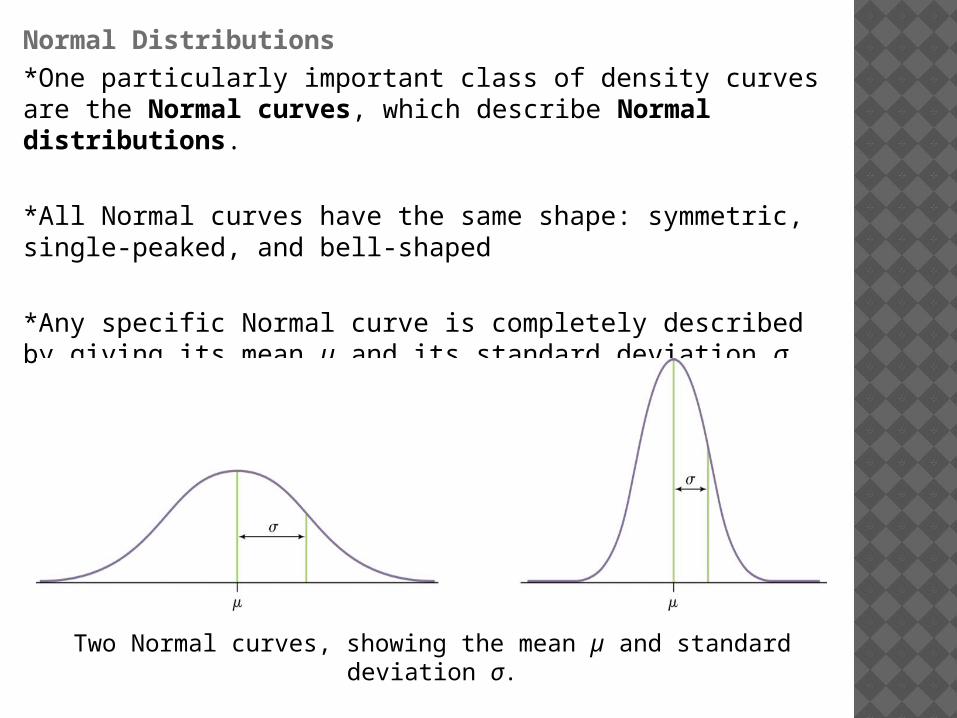
*One particularly important class of density curves are the Normal curves, which describe Normal distributions.

*All Normal curves have the same shape: symmetric, single-peaked, and bell-shaped

*Any specific Normal curve is completely described by giving its mean µ and its standard deviation σ.

Two Normal curves, showing the mean µ and standard deviation σ.

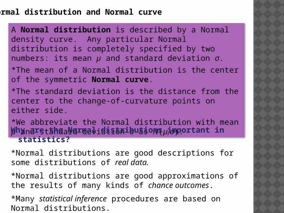
A Normal distribution is described by a Normal density curve. Any particular Normal distribution is completely specified by two numbers: its mean µ and standard deviation σ.

*The mean of a Normal distribution is the center of the symmetric Normal curve.

*The standard deviation is the distance from the center to the change-of-curvature points on either side.

*We abbreviate the Normal distribution with mean µ and standard deviation σ as N(µ,σ).

Why are the Normal distributions important in statistics?

*Normal distributions are good descriptions for some distributions of real data.

*Normal distributions are good approximations of the results of many kinds of chance outcomes.

*Many statistical inference procedures are based on Normal distributions.

Normal distribution and Normal curve

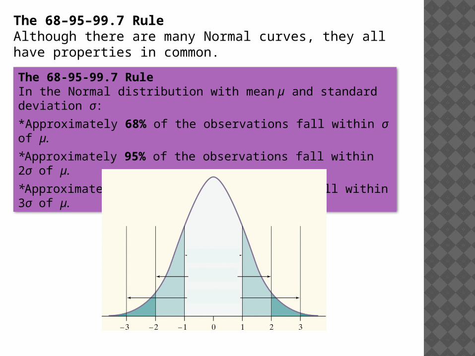
The 68–95–99.7 RuleAlthough there are many Normal curves, they all have properties in common.

The 68-95-99.7 RuleIn the Normal distribution with mean µ and standard deviation σ:

*Approximately 68% of the observations fall within σ of µ.

*Approximately 95% of the observations fall within 2σ of µ.

*Approximately 99.7% of the observations fall within 3σ of µ.

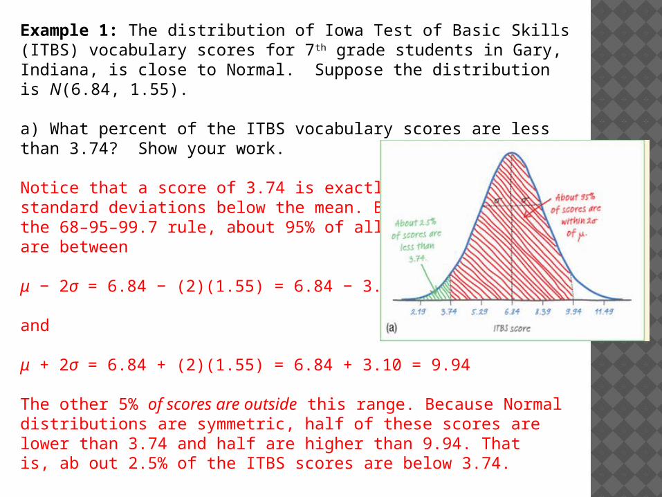
Example 1: The distribution of Iowa Test of Basic Skills (ITBS) vocabulary scores for 7th grade students in Gary, Indiana, is close to Normal. Suppose the distribution is N(6.84, 1.55). a) What percent of the ITBS vocabulary scores are less than 3.74? Show your work.

Notice that a score of 3.74 is exactly two standard deviations below the mean. By the 68–95–99.7 rule, about 95% of all scores are between

μ − 2σ = 6.84 − (2)(1.55) = 6.84 − 3.10 = 3.74

and

μ + 2σ = 6.84 + (2)(1.55) = 6.84 + 3.10 = 9.94

The other 5% of scores are outside this range. Because Normal distributions are symmetric, half of these scores are lower than 3.74 and half are higher than 9.94. That is, ab out 2.5% of the ITBS scores are below 3.74.

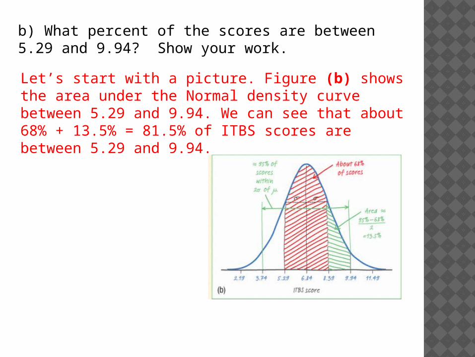
b) What percent of the scores are between 5.29 and 9.94? Show your work.

Let’s start with a picture. Figure (b) shows the area under the Normal density curve between 5.29 and 9.94. We can see that about 68% + 13.5% = 81.5% of ITBS scores are between 5.29 and 9.94.

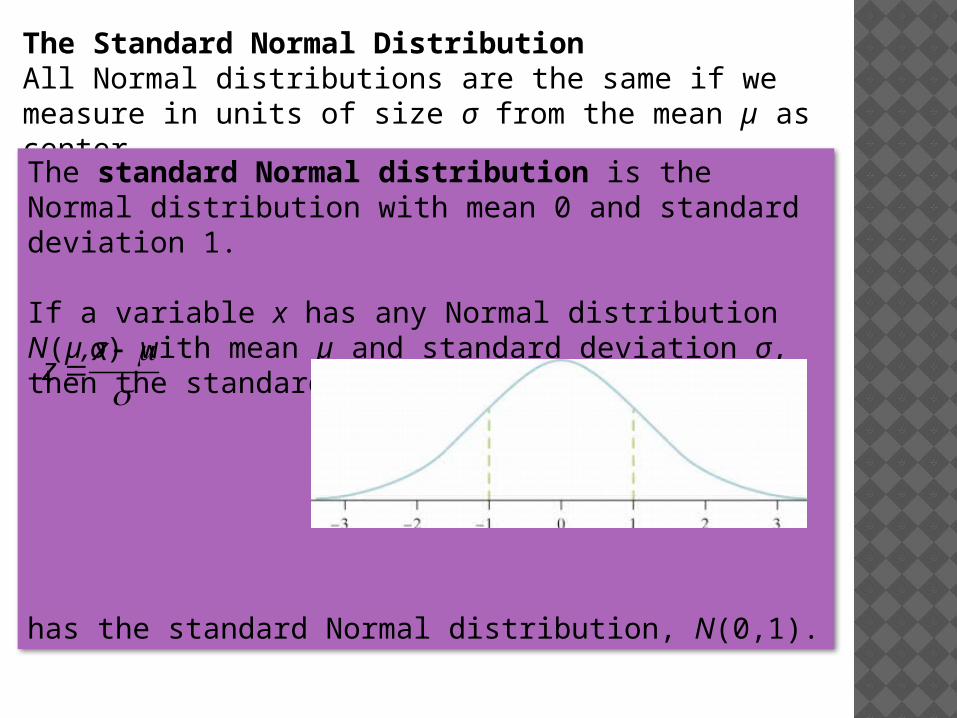
The Standard Normal Distribution All Normal distributions are the same if we measure in units of size σ from the mean µ as center.

The standard Normal distribution is the Normal distribution with mean 0 and standard deviation 1.

If a variable x has any Normal distribution N(µ,σ) with mean µ and standard deviation σ, then the standardized variable

has the standard Normal distribution, N(0,1).

xz

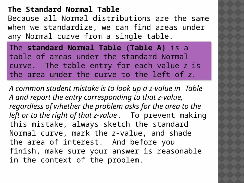
The standard Normal Table (Table A) is a table of areas under the standard Normal curve. The table entry for each value z is the area under the curve to the left of z.

The Standard Normal TableBecause all Normal distributions are the same when we standardize, we can find areas under any Normal curve from a single table.

A common student mistake is to look up a z-value in Table A and report the entry corresponding to that z-value, regardless of whether the problem asks for the area to the left or to the right of that z-value. To prevent making this mistake, always sketch the standard Normal curve, mark the z-value, and shade the area of interest. And before you finish, make sure your answer is reasonable in the context of the problem.

Z .00 .01 .02

0.7 .7580 .7611 .7642

0.8 .7881 .7910 .7939

0.9 .8159 .8186 .8212

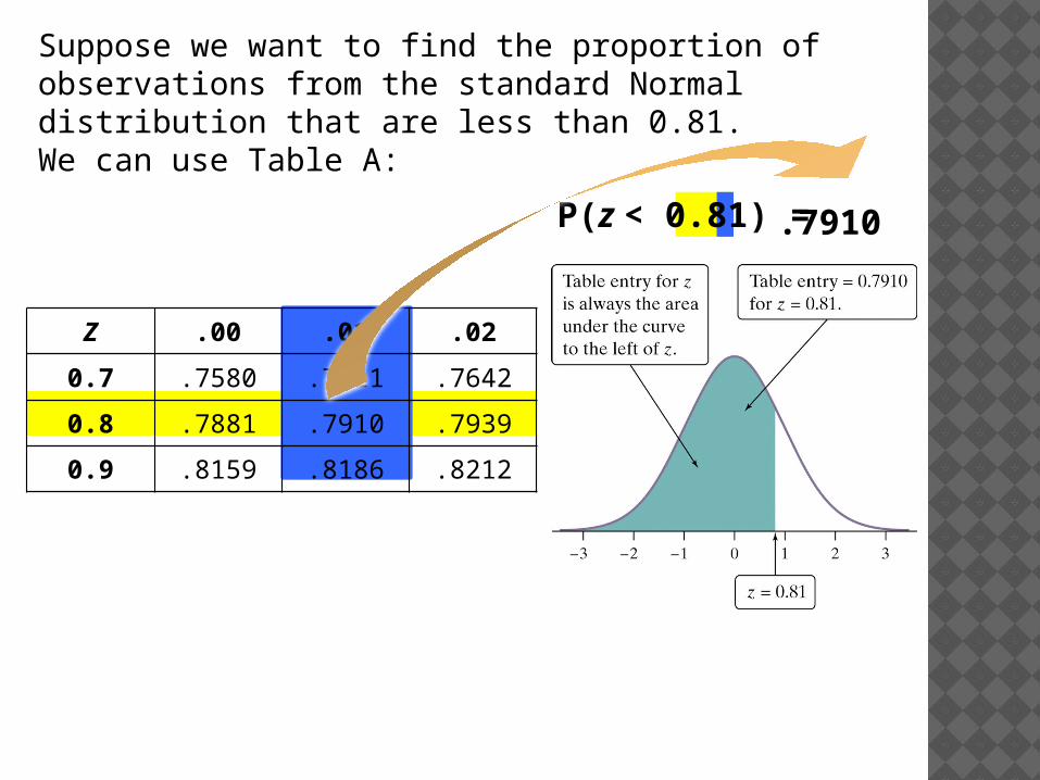
P(z < 0.81) = .7910

Suppose we want to find the proportion of observations from the standard Normal distribution that are less than 0.81. We can use Table A:

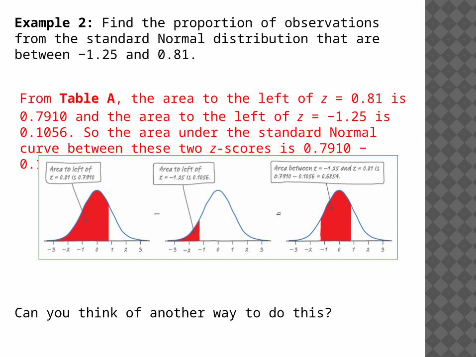
Example 2: Find the proportion of observations from the standard Normal distribution that are between −1.25 and 0.81.

Can you think of another way to do this?

From Table A, the area to the left of z = 0.81 is 0.7910 and the area to the left of z = −1.25 is 0.1056. So the area under the standard Normal curve between these two z-scores is 0.7910 − 0.1056 = 0.6854. 

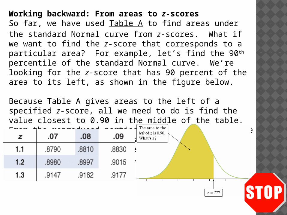
Working backward: From areas to z-scoresSo far, we have used Table A to find areas under the standard Normal curve from z-scores.  What if we want to find the z-score that corresponds to a particular area?  For example, let’s find the 90th percentile of the standard Normal curve.  We’re looking for the z-score that has 90 percent of the area to its left, as shown in the figure below. Because Table A gives areas to the left of a specified z-score, all we need to do is find the value closest to 0.90 in the middle of the table.  From the reproduced portion of Table A, you can see that the desired z-score is z = 1.28.  That is, the area to the left of z = 1.28 is approximately 0.90.

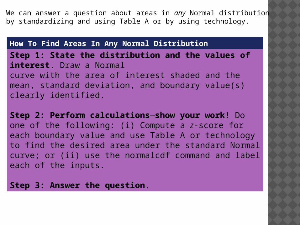
We can answer a question about areas in any Normal distribution by standardizing and using Table A or by using technology.

Step 1: State the distribution and the values of interest. Draw a Normalcurve with the area of interest shaded and the mean, standard deviation, and boundary value(s) clearly identified.

Step 2: Perform calculations—show your work! Do one of the following: (i) Compute a z-score for each boundary value and use Table A or technology to find the desired area under the standard Normal curve; or (ii) use the normalcdf command and label each of the inputs.

Step 3: Answer the question.

How To Find Areas In Any Normal Distribution

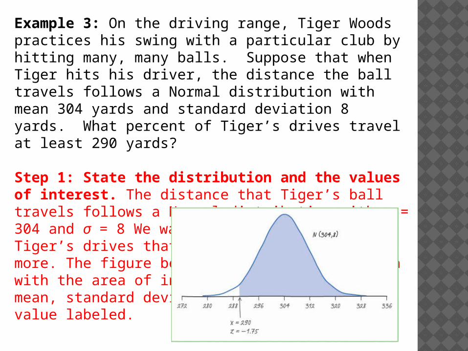
Example 3: On the driving range, Tiger Woods practices his swing with a particular club by hitting many, many balls.  Suppose that when Tiger hits his driver, the distance the ball travels follows a Normal distribution with mean 304 yards and standard deviation 8 yards.  What percent of Tiger’s drives travel at least 290 yards?

Step 1: State the distribution and the values of interest. The distance that Tiger’s ball travels follows a Normal distribution with μ = 304 and σ = 8 We want to find the percent of Tiger’s drives that travel 290 yards or more. The figure below shows the distribution with the area of interest shaded and the mean, standard deviation, and boundary value labeled.

Step 2: Perform calculations–show your work! For the boundary value x = 290,we have

So drives of 290 yards or more correspond to z ≥ −1.75 under the standard Normal curve.

From Table A, we see that the proportion of observations less than −1.75 is 0.0401.The area to the right of −1.75 is therefore 1 − 0.0401 = 0.9599. This is about 0.96,or 96%.

Using technology: The command normalcdf(lower:2 90, upper:100000, μ:304, σ:8)also gives an area of 0.9599.

Step 3: Answer the question. About 96% of Tiger Woods’s drives on the range travel at least 290 yards.

290 3041.75

8

xz

In a Normal distribution, the proportion of observations with x ≥ 290 is the same as the proportion with x > 290. There is no area under the curve exactly above the point 290 on the horizontal axis, so the areas under the curve with x ≥ 290 and x > 290 are the same. This isn’t true of the actual data. Tiger may hit a drive exactly 290 yards. The Normal distribution is just an easy-to-use approximation, not a description of every detail in the actual data. The key to doing a Normal calculation is to sketch the area you want, then match that area with the area that the table gives you.

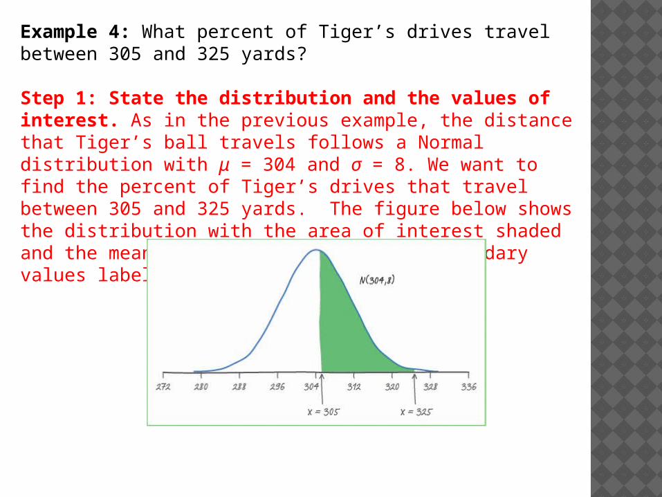
Example 4: What percent of Tiger’s drives travel between 305 and 325 yards?

Step 1: State the distribution and the values of interest. As in the previous example, the distance that Tiger’s ball travels follows a Normal distribution with μ = 304 and σ = 8. We want to find the percent of Tiger’s drives that travel between 305 and 325 yards. The figure below shows the distribution with the area of interest shaded and the mean, standard deviation, and boundary values labeled.

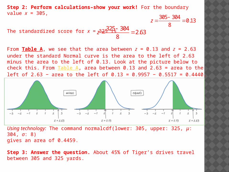
Step 2: Perform calculations–show your work! For the boundary value x = 305,  

The standardized score for x = 325 is 

From Table A, we see that the area between z = 0.13 and z = 2.63 under the standard Normal curve is the area to the left of 2.63 minus the area to the left of 0.13. Look at the picture below to check this. From Table A, area between 0.13 and 2.63 = area to the left of 2.63 − area to the left of 0.13 = 0.9957 − 0.5517 = 0.4440.

Using technology: The command normalcdf(lower: 305, upper: 325, μ: 304, σ: 8) gives an area of 0.4459.

Step 3: Answer the question. About 45% of Tiger’s drives travel between 305 and 325 yards.

305 3040.13

8z

325 3042.63

8z

How to Find Values from Areas in Any Normal Distribution Step 1: State the distribution and the values of interest. Draw a Normal curve with the area of interest shaded and the mean, standard deviation, and unknown boundary value clearly identified. Step 2: Perform calculations – show your work! Do one of the following: (i) Use Table A or technology to find the value z with the indicated area under the standard Normal curve, then “unstandardized” to transform back to the original distribution; or (ii) Use the invNorm command and label each of the inputs. Step 3: Answer the question.

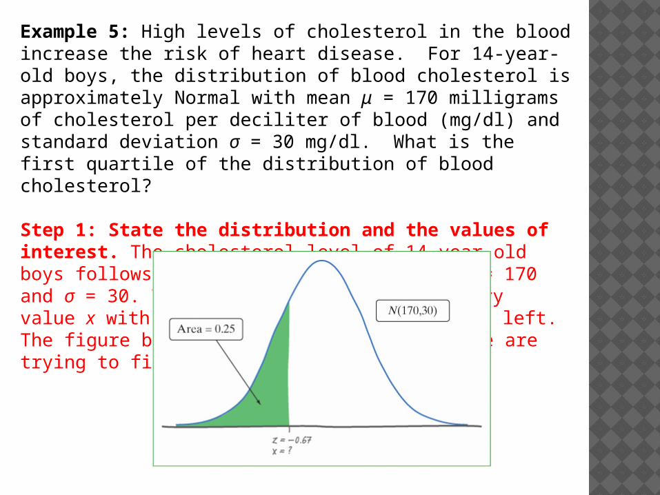
Example 5: High levels of cholesterol in the blood increase the risk of heart disease. For 14-year-old boys, the distribution of blood cholesterol is approximately Normal with mean μ = 170 milligrams of cholesterol per deciliter of blood (mg/dl) and standard deviation σ = 30 mg/dl. What is the first quartile of the distribution of blood cholesterol?

Step 1: State the distribution and the values of interest. The cholesterol level of 14-year-old boys follows a Normal distribution with μ = 170 and σ = 30. The 1st quartile is the boundary value x with 25% of the distribution to its left. The figure below shows a picture of what we are trying to find.

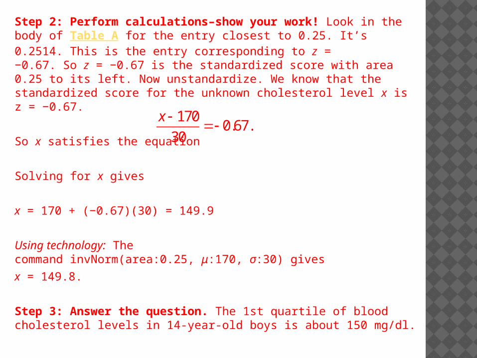
Step 2: Perform calculations–show your work! Look in the body of Table A for the entry closest to 0.25. It’s 0.2514. This is the entry corresponding to z = −0.67. So z = −0.67 is the standardized score with area 0.25 to its left. Now unstandardize. We know that the standardized score for the unknown cholesterol level x is z = −0.67.

So x satisfies the equation  

Solving for x gives

x = 170 + (−0.67)(30) = 149.9

Using technology: The command invNorm(area:0.25, μ:170, σ:30) gives 

x = 149.8.

Step 3: Answer the question. The 1st quartile of blood cholesterol levels in 14-year-old boys is about 150 mg/dl.

1700.67.

30

x

Assessing Normality

The Normal distributions provide good models for some distributions of real data. Many statistical inference procedures are based on the assumption that the population is approximately Normally distributed. Consequently, we need a strategy for assessing Normality.

Plot the data.

*Make a dotplot, stemplot, or histogram and see if the graph is approximately symmetric and bell-shaped.

 

Check whether the data follow the 68-95-99.7 rule.

*Count how many observations fall within one, two, and three standard deviations of the mean and check to see if these percents are close to the 68%, 95%, and 99.7% targets for a Normal distribution.

 

 

Normal Probability Plots

Most software packages can construct Normal probability plots. These plots are constructed by plotting each observation in a data set against its corresponding percentile’s z-score.

 

 

AP EXAM TIP: Normal probability plots are not included on the AP Statistics course outline. However, these graphs are very useful tools for assessing Normality. You may use them on the AP exam if you wish—just be sure that you know what you’re looking for (linear pattern).

A Normal probability plot provides a good assessment of whether a data set follows a Normal distribution.

If the points on a Normal probability plot lie close to a straight line, the plot indicates that the data are Normal.

Systematic deviations from a straight line indicate a non-Normal distribution.

Outliers appear as points that are far away from the overall pattern of the plot.

Interpreting Normal Probability Plots

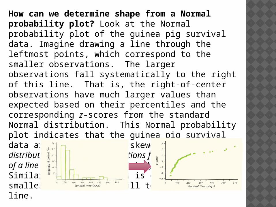
How can we determine shape from a Normal probability plot? Look at the Normal probability plot of the guinea pig survival data. Imagine drawing a line through the leftmost points, which correspond to the smaller observations. The larger observations fall systematically to the right of this line. That is, the right-of-center observations have much larger values than expected based on their percentiles and the corresponding z-scores from the standard Normal distribution. This Normal probability plot indicates that the guinea pig survival data are strongly right-skewed. In a right-skewed distribution, the largest observations fall distinctly to the right of a line drawn through the main body of points. Similarly, left-skewness is evident when the smallest observations fall to the left the line.