2.2 BUDGET-CONSTRAINED CHOICE WITH TWO COMMODITIESessentialmicroeconomics.com/ChapterY2/SlideChapter2-2.pdf · 2.2 BUDGET-CONSTRAINED CHOICE WITH TWO COMMODITIES ... Essential Microeconomics

Essential Microeconomics -1-

© John Riley October 4, 2014

2.2 BUDGET-CONSTRAINED CHOICE WITH TWO COMMODITIES

Continuity of demand 2

Income effects 6

Quasi-linear, Cobb-Douglas and CES preferences 9

Expenditure function 14

Substitution effects and Compensated demand 17

Elasticity of substitution 19

Determinants of demand elasticity 25



Consider the choice problem of a consumer with income I facing a price vector p.

{ ( ) | , }n

xMax U x p x I x (2.2-1)

We assume that the local non-satiation assumption holds and that the utility function is continuous and

strictly quasi-concave on 2 . The local non-satiation assumption ensures that the consumer spends all

his or her income and strict quasi-concavity ensures that there is a unique1 solution 0 ( , )x x p I .

__________

1Suppose 0x and

1x are both solutions. Then 0 1( ) ( )U x U x and because U is strictly quasi-concave it follows

that for any convex combination 0, ( ) ( )x U x U x . Finally, because

0p x I and 1p x I , then

p x I . Thus x is feasible and strictly preferred.



Given uniqueness and continuity of preferences, it is intuitively plausible that the implied demand

function ( , )x p I must be continuous. This follows from the Theorem of the Maximum (See EM

Appendix C.)

Proposition 2.2-1: Theorem of the Maximum (I)

Consider the maximization problem

{ ( , ) | ( ), }x

Max f x x X A where ( ) { , ( , ) 0, 1,..., }niX x h x i m .

If f and ( )X are continuous1 and, for all , there is a unique solution ( )x , then ( )x is continuous.

For the most general propositions about consumers (and firms as well) continuity is all that we need.

However, to simplify modeling, it is convenient to assume some degree of differentiability as well.

Then the necessary conditions for a maximum are restrictions on the gradient vector of the maximand

and constraint functions.

_______ 1 The mapping from a parameter to a set is called a correspondence. For a formal definition of a continuous

correspondence, see EM Appendix C.



Assumptions

Differentiability: The utility function is continuously differentiable on 2 .

Strictly increasing preferences: For all , ( ) 0n Ux x

x

.

Whenever we wish to avoid corner solutions we also assume that 0

lim , 1,...,jx

j

Uj n

x

.

Forming the Lagrangian for the maximization problem (2.2-1),

( )U I p x L .

FOC

*( ) 0, 1,...,j

j j

Ux p j n

x x

L, with equality if 0jx

Note that because the marginal utility of at least one commodity is strictly positive, the shadow price

(or marginal utility of income) must be strictly positive.



Henceforth we will focus primarily on the simplest 2 commodity case. If both commodities are

consumed, the FOC can be rewritten as follows.

1 2

1 2

U U

x x

p p

. (2.2-2)

One extra dollar spent on commodity 1 yields 1

1

p additional units thus the marginal value per dollar

spent on commodity 1 is 1 1

1 U

p x

. Spending on commodity 1 is increased until this is equal to the

marginal value of spending an additional dollar on commodity 2. We can also rewrite the FOC as

follows:

* 1 1

2

2

( )

U

x pMRS x

U p

x

.

That is, the slope of the indifference curve must equal

the slope of the budget line in Figure 2.2-1.

Figure 2.2-1: Budget constrained choice



Income Effects

Figure 2.2-2 shows the path of the consumer’s choice

* ( , )x x p I as his income increases. As shown, this

“Income Expansion Path” is initially positively sloped

i.e. 1x

I

and 2x

I

are both positive.

In this case the commodities are said to be normal in the

neighborhood of the optimum.

However, as depicted, for higher incomes consumption of commodity 1 declines as income increases.

In this case commodity 1 is “inferior” in the neighborhood of the optimum.

To facilitate comparisons across commodities, it is helpful to consider the proportional effects on

demand as income changes, in other words the income elasticity of demand

( , )j

j

j

xIx I

x I

.

Figure 2.2-2: Income Expansion Path



In Figure 2.2-2 the slope of the Income Expansion path at * ( , )x x p I is steeper than the line

joining *x and the origin, that is

2*

2 2

*11 1IEP

xdx xI

xdx x

I

.

Rearranging this inequality,

2 12 1* *

2 1

( , ) ( , )x xI I

x I x II Ix x

.

Appealing to the following lemma, the income elasticities

weighted by their expenditure shares must sum to 1. Thus, in Figure 2.2-2, the income elasticity of

demand for commodity 2 exceeds 1 and for commodity 1 is less than 1.

Lemma 2.2-2: Income Elasticities Weighted by Expenditure Shares Sum to 1

* *1 1 2 2( , ) ( , ) 1k x I k x I

where

*j j

j

p xk

I is the expenditure share for commodity j.

Figure 2.2-2: Income Expansion Path



Proof: To establish this proposition, we substitute the consumer’s choice into the budget constraint and

differentiate by I.

* *1 2

1 2 1x x

p pI I

.

Rearranging the left-hand side,

* * * *

* *1 1 1 2 2 21 1 2 2* *

1 2

( ) ( ) ( , ) ( , ) 1p x x p x xI I

k x I k x II I I Ix x

.

Q.E.D.



We now examine income elasticities for three commonly used utility functions.

Example 1: Quasi-Linear Preferences

Definition: Preferences are quasi-linear if they can be represented by the utility function

1 2( ) ( )U x v x x .

For such a utility function the marginal rate of substitution (MRS) at *x is

*

*2 1 1

1 ( )

2

( )

U U x

U

dx x v x

Udx

x

.

The MRS is independent of commodity 2 which means that

the indifference curves are vertically parallel.

As depicted in Figure 2.2-3, it follows that the income

expansion path is first horizontal and then vertical.

Over the range in which both commodities are consumed, it follows that the income elasticity of

commodity 1 is zero. Given Lemma 2.2-2, the income elasticity of commodity 2 is the inverse of the

expenditure share. █

Income

Expansion Path

Figure 2-2-3: Quasi-linear preferences



Example 2: Cobb-Douglas Preferences1 1 21 2 1 2( ) , , 0U x x x

Differentiating by 1x , 1 21 11 1 2

1 1

UUx x

x x

. Similarly, 2

2 2

UU

x x

.

At the maximum the FOC must be satisfied, hence

1 2

1 2

U U

x x

p p

.

Substituting and then dividing by U ,

1 2

1 1 2 2p x p x U

,

hence j

j jp x

.

____

1Since 1 1 2 2( ) ln ( ) ln lnu x U x x x , ( )U x is strictly quasi-concave and so the FOC are sufficient.



We then solve for by substituting back into the budget constraint.

1 21 1 2 2p x p x I

, hence 1 2

I

.

Demand for commodity j is therefore 1 2

( , )j

j

j

Ix p I

p

.

Finally, substituting back into the utility function, maximized utility is

1 2 1 21 2

1 2 1 2

( ( , )) ( ) ( ) ( )I

U x p Ip p

. █



Example 3: CES Preferences 1 1 1

1

1 1 1

1 1 2 2 1 2( ) ( ) , , , 0, 1U x x x

From the definition of U,

1 11 1 11

1 1 2 2( )U x x x

.

Differentiating by jx ,

1 1

1 1(1 ) (1 ) j j

j

UU x

x

. Hence

1

1

j

j

j

UU

xx

.

We follow the same steps as for Example 2.

Substituting into the FOC and then dividing by

1

U ,

1 2

1 1 1

1 1 2 2p x p x U

. (2.2-3)

Hence ( )j

j

j

xp

and so

1j j

j j

pp x

.



We then solve for by substituting back into the budget constraint

1 11 1 2 2 1 1 2 2

1( )p x p x p p I

, hence 1 1

1 1 2 2

1 I

p p

.

Demand for commodity j is therefore

1

1 11 1 2 2

( , ) ( )j j

j

j

pIx p I

p p p

. (2.2-4)

Substituting ( , )x p I into the utility function and collecting terms,

1

1 1 11 1 2 2

( ( , ))

( )

IU x p I

p p

.

Note that the demand functions given by (2.2-4) reduce to the Cobb-Douglas

demand functions if 1 . █

Note: For 1 , maximizing ( )U x is equivalent to minimizing 1 11 1

1 1 2 2( )v x x x

which, in turn, is

equivalent to maximizing the concave function 1 11 1

1 1 2 2( )u x x x

. Thus the necessary conditions are

sufficient.



Dual optimization problem: expenditure minimization

Given the very weak assumption of local non-satiation,

for any budget constrained utility maximization problem

there is a “dual” optimization problem.

As we shall see, this dual problem is very useful in

understanding the determinants of demand.

Suppose that *x is a solution to a consumer’s maximization

problem. That is,

* arg { ( ) | 0, }x

x Max U x x p x I .

Such a consumption bundle is depicted in Figure 2.2-4.

Figure 2.2-4: Expenditure Minimization



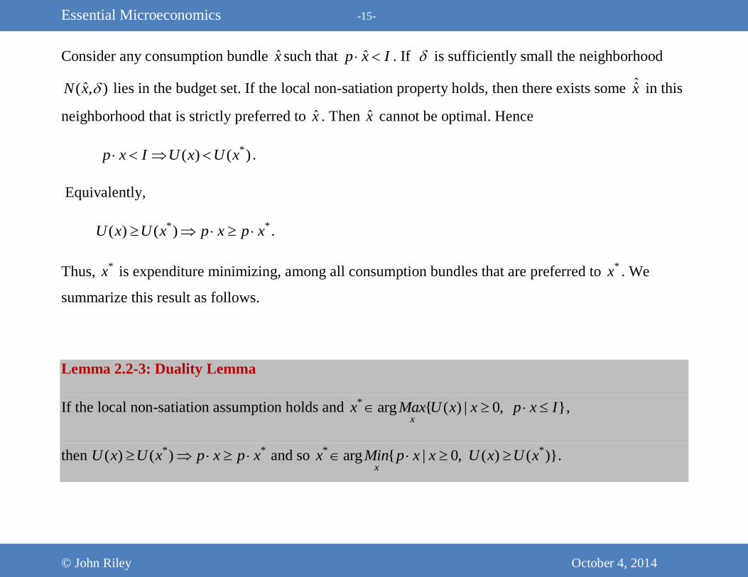
Consider any consumption bundle x such that ˆp x I . If is sufficiently small the neighborhood

ˆ( , )N x lies in the budget set. If the local non-satiation property holds, then there exists some ˆx in this

neighborhood that is strictly preferred to x . Then x cannot be optimal. Hence

*( ) ( )p x I U x U x .

Equivalently,

* *( ) ( )U x U x p x p x .

Thus, *x is expenditure minimizing, among all consumption bundles that are preferred to *x . We

summarize this result as follows.

Lemma 2.2-3: Duality Lemma

If the local non-satiation assumption holds and * arg { ( ) | 0, }x

x Max U x x p x I ,

then * *( ) ( )U x U x p x p x and so * *arg { | 0, ( ) ( )}x

x Min p x x U x U x .



For any level of utility, U and price vector p we define the expenditure function ( , )M p U to be the

minimum expenditure needed to achieve the utility level U .

Definition: Expenditure Function

( , ) { | ( ) }x

M p U Min p x U x U

While it is not difficult to solve for the expenditure function,

it is often more convenient to solve first for the

indirect utility function

( , ) { ( ) | }x

V p I Max U x p x I .

Given local non-satiation, the consumer spends his entire

income.

Moreover the higher his income the greater is his utility.

Thus maximized utility ( , )V p I is a strictly increasing function of income. This is depicted in Figure

2.2-5. The expenditure function is then the inverse mapping from U to I.

Figure 2.2-5: Maximized utility as a function of income



Compensated demand

Let ( , )cx p U be the solution to the dual problem, that is ( , )cx p U solves

( , ) { | ( ) }x

M p U Min p x U x U

This is known as the consumer’s compensated demand. Consider the effect on compensated demand of

an increase in the price of commodity 1. This is depicted in Figure 2.2-6 for price vectors 0p and

1p .

As the price of commodity 1 rises, the consumer is compensated so that he is just able to maintain the

utility level 0U .

Figure 2.2-6: Substitution effect



The following useful property of the expenditure function is an immediate implication of the Envelope

Theorem.1

0( , )cMx p U

p

Informally, if the price of commodity j rises and the consumer maintains his consumption plan, his

extra expenditure is *jx . This is the direct effect. The indirect effect associated with adjusting to the

change in the price is of second order.

____

1 See Exercise 2.2-2. Converting the expenditure minimization problem to a maximization problem, ( ( ) )p x U x U L

so j

j j

Mx

p p

L.



Substitution Effect

The effect on demand of a compensated price change is called the substitution effect. As Figure 2.2-6

illustrates, the size of this effect depends critically on the curvature of the indifference curve. In the

left diagram, as the price ratio changes, the consumption ratio 0

2

01

( , )

( , )

c

c

x p U

x p U changes a lot. That is, the

substitution effect is large. In the right diagram a price change has a small effect on the consumption

ratio so the substitution effect is small. As we shall see, the elasticity of the consumption ratio with

respect to the price ratio is a very useful measure of price sensitivity.

Definition: Elasticity of substitution 2 1

21

( , )c

c

x p

px .

Example: CES utility function

From equation (2.2-3), 2 2 1

1 1 2

c

c

x p

x p

.

Taking the logarithm,

2 1

21

ln( ) ln( )c

c

x p

px constant.



As is readily confirmed, ( , ) lnd

y x x ydx

. Hence, 2 1

21

( , )c

c

x p

px .

Thus for the CES utility function, the parameter is the elasticity of substitution.

█

Quick review of elasticity

For any function ( )y f x let y be the change in y when the change in x is x . A measure of the

sensitivity of y with respect to x is the percentage change in y divided by the percentage change in x.

100 /100y x x y

y x y x

An advantage of this measure is that it is independent of the units in which the two variable are

measured. To see this suppose we rescale units so that x x and y y . Then

ˆ ˆ

ˆ ˆ

x y x y

y x y x

.



(Point) Elasticity

We define the point elasticity to the limit as 0x

0( , ) lim

x

x y x dyy x

y x y dx

.

Then from the above observation ( , ) ( , )y x y x

Note that 1

lnd dy

ydx y dx

. Therefore the point elasticity can be rewritten as follows:

( , ) lnx dy d

y x x yy dx dx

.

The following lemma is an immediate implication.

Lemma 2.2-4:

2 12 1 1 1

21

( , ) ( , ) ( , )c

c c

c

x px p x p

px

We appeal to this lemma in proving the following result.



Proposition 2.2-5: Elasticity of Substitution and Compensated Own Price Elasticity

2 1

1

( , )cx p

k

where 1 1

1

p xk

p x

and

1 1 1( , ) (1 )cx p k

Proof: To demonstrate equivalence, first note that around the indifference curve as 1p rises we have

1 2

1 1 2 1

0c cx xU U

x p x p

.

Also, from the first order condition, the marginal utility of each commodity is proportional to its price.

Hence

1 21 2

1 1

0c cx x

p pp p

. (2.2-5)

Dividing by 1cx and rearranging this equation,

1 1 2 2 2 2 1 2

1 1 11 1 1 1 2

( )c c c c

c c c c

p x p x p x p x

p p px x p x x

2 1 2

1 12

c

c

k p x

k px

, where /c c

j j jk p x p x .



Therefore

21 1 2 1

1

( , ) ( , )c ckx p x p

k . (2.2-6)

From Lemma 2.2-4,

2 1 1 1( , ) ( , )c cx p x p .

From (2.2-6), 21 1 2 1

1

( , ) ( , )c ckx p x p

k .

Substituting for the second term on the right hand side

22 1 2 1 2 1

1 1

1( , ) ( , ) ( , )c c ckx p x p x p

k k .

Substituting this expression into (2.2-6),

1 1 2 1( , ) (1 )cx p k k .

Q.E.D.



Remark: Note that the compensated own price elasticity, 1 1 1( , ) (1 )cx p k , is bounded from

below by the elasticity of substitution. Moreover, if the expenditure share is small, the elasticity of

substitution is a good approximation for the compensated own price elasticity.

Decomposition of price effects

To understand the impact of a price

change it proves helpful to decompose this

into two parts: a compensated price effect

and an income effect. Consider the figure.

The left hand diagram illustrates the effect

of an increase in the price of commodity 1.

Suppose next that the individual is fully

compensated as the price rises. In the right hand diagram in Figure 2.2-7 the consumer moves along his

indifference curve from A to C substituting commodity 2 for commodity 1. This is the substitution

O

A B

O

B

C

A

Figure 2.2-7: Decomposition of the price effect into income and substitution effects



effect of the price increase. In the second step, the extra compensation is taken away and the budget

line is pulled in towards the origin. The consumer then moves from C to B. Note that if, as depicted,

commodity 1 is a normal good, both the substitution and income effects are negative. That is, the

bigger (i.e. the more negative) the substitution effect and the bigger the income effect, the greater will

be the total effect on demand for commodity 1.

Slutsky Equation

We now consider the decomposition of the price effect in mathematical terms. If ( , )M p U is

minimized total expenditure at utility level U , and 1( , )x p I is the consumer’s demand for commodity

1, the compensated demand is 1 1( , ( , ))cx x p M p U . Differentiating by 1p , the slope of the

compensated demand curve is

1 1 1

1 1 1

cx x x M

p p I p

Yet we have seen that 1

1

Mx

p

. Substituting into the above expression and rearranging,



1

1 1

cj j j

incometotal price compensatedeffecteffect price effect

x x xx

p p I

. Slutsky equation

In particular, the Slutsky decomposition of the "own price effect" is as follows:

1 1 11

1 1

cx x xx

p p I

. (2.2-7)

Determinants of Demand Price Elasticity

Using the Slutsky equation, we can develop insights into the determinants of demand elasticity.

Converting (2.2-7) into elasticity form,

1 1 1 1 1 1 1

1 1 1 1 1

cp x p x p x xI

x p x p I x I

.

where 1 1 ( , )c cx x p U is the compensated demand for commodity 1. Hence

1 1 1 1 1 1( , ) ( , ) ( , )cx p x p k x I . (2.2-8)

From Proposition 2.2-5, 1 1 1( , ) (1 )cx p k .



Substituting for 1 1( , )cx p in equation (2.2-8) we have the following proposition.

Proposition 2.2-6: Decomposition of Own Price Elasticity

1 1 1 1 1( , ) (1 ) ( , )x p k k x I

It follows that the absolute value of the own price elasticity must lie between the income elasticity and

the elasticity of substitution. Holding the expenditure share constant, the higher the elasticity of

substitution or the income elasticity, the more negative is the own price elasticity. Moreover, the higher

the expenditure share of commodity 1, the greater the weight on the income elasticity. Intuitively, a

higher share means that a price rise requires a bigger change in income for the individual to be

compensated. Thus the income effect on the change in demand is greater.

Documents

2.2 BUDGET-CONSTRAINED CHOICE WITH TWO COMMODITIESessentialmicroeconomics.com/ChapterY2/SlideChapter2-2.pdf · 2.2 BUDGET-CONSTRAINED CHOICE WITH TWO COMMODITIES ... Essential Microeconomics