212 Years of Price Momentum

(The World’s Longest Backtest: 1801 – 2012)

CHRISTOPHER GECZY and MIKHAIL SAMONOV

ABSTRACT

We assemble a dataset of U.S. security prices between 1801 and 1926, and create an out-

of-sample test of the price momentum strategy, discovered in the post-1927 data. The

pre-1927 momentum profits remain positive and statistically significant. Additional time

series data strengthens the evidence that momentum is dynamically exposed to market

beta, conditional on the sign and duration of the tailing market state. In the beginning of

each market state, momentum’s beta is opposite from the new market direction,

generating a negative contribution to momentum profits around market turning points. A

dynamically hedged momentum strategy significantly outperforms the un-hedged

strategy.

*The authors thank William Goetzmann, Roger Ibbotson, Liang Peng, Charles Jones, Eugene Fama, Kenneth French, Michael Halperin and Bryan Taylor. We also thank the International Center of Finance at Yale and the Inter-University Consortium for Political and Social Research. Data available at www.octoquant.com

   

    2  

The first two U.S. stocks traded hands in 1792 in New York. Over the following

decades, the security market developed rapidly. By the end of 1810, 72 traded securities

existed, and by the end of 1830s the number was over 300. To our knowledge, all current

academic studies of U.S. security-level data begin in 1926, the year the CRSP database

began. The U.S. market had been active for 133 years before that time, providing an

opportunity to test stock-level studies in earlier history. The 19th and early 20th centuries

are filled with expansions, recessions, wars, panics, manias, and crashes, all providing a

rich out-of-sample history. Limiting studies to the post-1925 period introduces a strong

selection bias and does not capture the full distribution of possible outcomes.

For example, in the case of price momentum, before 2009, only following the

Great Depression did the strategy have a decade-long negative compounded return. Such

occurrence was concluded to be an outlier and the remaining part of the distribution taken

as normal. Since 2009, second worst financial collapse, momentum has experienced

another decade long underperformance creating a large ripple in investment portfolios

that use this strategy. The repeated underperformance raised practical questions about the

outlier conclusion and what the actual distribution of momentum profits is. By extending

the momentum data back to 1801, we create a more complete picture of the potential

outcomes of momentum profits, discovering 7 additional negative decade long periods

prior to 1925.

The first contribution of this study is a creation of a monthly stock price dataset.

In this dataset, three known 19th and early 20th century data sources are combined into

one testable dataset from 1800 to 1927. Those data sources are: the International Center

of Finance at Yale (ICF); the Inter-University Consortium for Political and Social

   

    3  

Research (ICPSR); and Global Financial Data (GFD). Between 1800 and 1927, the

merged dataset contains an average of 272 securities per month, making it robust for

security level studies.

The second contribution of this study is to add to the existing price momentum

literature by extending the momentum tests to the new data. Our study finds that in the

pre-1927 data, the momentum effect remains statistically significant and is about half the

post-1927 period. From 1801 to 1926, the equally weighted top third of stocks sorted on

price momentum out-performs the bottom third by 0.28% per month (t-stat 2.7),

compared to 0.58% per month (t-stat 3.6) for the 1927-2012 period. Linking the two

periods together generates a 212-year history of momentum returns, averaging of 0.4%

per month (t-stat 5.7).

As observed in the studies of the 20th century data, momentum profits are highly

variable over time, giving rise to the limits of arbitrage explanation. Nevertheless, over

the long run, the trend following strategy would have generated significant market

outperformance, in a different century than the one in which it was discovered and tested.

Our study adds to the evidence that momentum effect is not a product of data-mining but

it is highly variable overtime.

The third contribution of this study is to link momentum’s beta exposure to the

market state duration. We find strong evidence that momentum beta is positively

exposed to the duration of both positive and negative market states. The longer a given

market state persists, the stronger the momentum portfolio beta exposure becomes.

Analyzing the longer history is especially useful for the time-series tests, as the sample

size is more than doubled.

   

    4  

Using a 10-month return definition of a market state, we find 116 discrete states

in the full sample, with 69 of them in the pre-1927 period. We find strong evidence that

momentum beta is dynamic not only across both up and down market states, but also

within a given market state. In the first year of a given up or down market state,

momentum’s beta exposure generates a negative contribution to the momentum returns,

while momentum’s alpha exposure is significantly positive during this time. In market

states that last longer than one year, momentum’s beta becomes a positive contributor to

returns, while alpha contribution gradually declines. As a result, over the course of a

market state, momentum transforms from a purely stock-specific to a combination of

common-risk and stock specific strategy.

We find that both industry-neutral momentum and industry-level momentum are

priced. Additionally, we find that individual macro-economic variables do not explain

momentum. However, the market states, which arguably encompass and lead the

macroeconomic data, do significantly impact the nature of momentum profits, even as

alphas remain significant.

The rest of the paper is organized as follows. Section I describes the pre-1927

data assembly process; Section II uses the early security data to test the price momentum

effect; Section III provides a decomposition of momentum profits into common and

stock-specific components.

I. Early Security Returns Data

A series of academic efforts extended aggregate stock market returns back to

1792, the inception of the U.S. stock market. While some of these studies work with

   

    5  

already created indices (Schwert (1990), Siegel (1992), Shiller (2000), Wilson, Jones

(2000)), others assemble individual security prices into datasets from which aggregate

level returns are computed (Cowles (1939), Goetzmann, Ibbotson, Peng (2001), Sylla,

Wilson, Wright (2006), Global Financial Data). While the original stock-level Cowles

data files seem to be lost1, the other datasets are preserved; however, they vary from each

other both in the securities and the periods they cover.

Return estimation and index construction methodologies also vary among studies.

For example, Schwert (1990) uses spliced index data from Cole and Smith (1935);

Macaulay (1938); Cowles (1939); and Dow Jones (1975). As a result, their index is

equally weighted before 1862, value weighted from 1863 to 1885, and price weighted

between 1885 and 1925. Goetzmann et al. (2001) use price weighted index construction

over the entire period to avoid the large bid-ask bounce effect in the 19th century prices

that effects equally weighted returns. Another difference between approaches is the use

of month-end (Goetzmann et al. 2001) versus an average of high and low prices within

the month (Cowles, 1939, GFD).

Our 1800-1926 dataset of security prices (hereafter Merged) and industry

classifications is created from three sources: International Center of Finance at Yale

(ICF); Inter-University Consortium for Political and Social Research (ICPSR); and

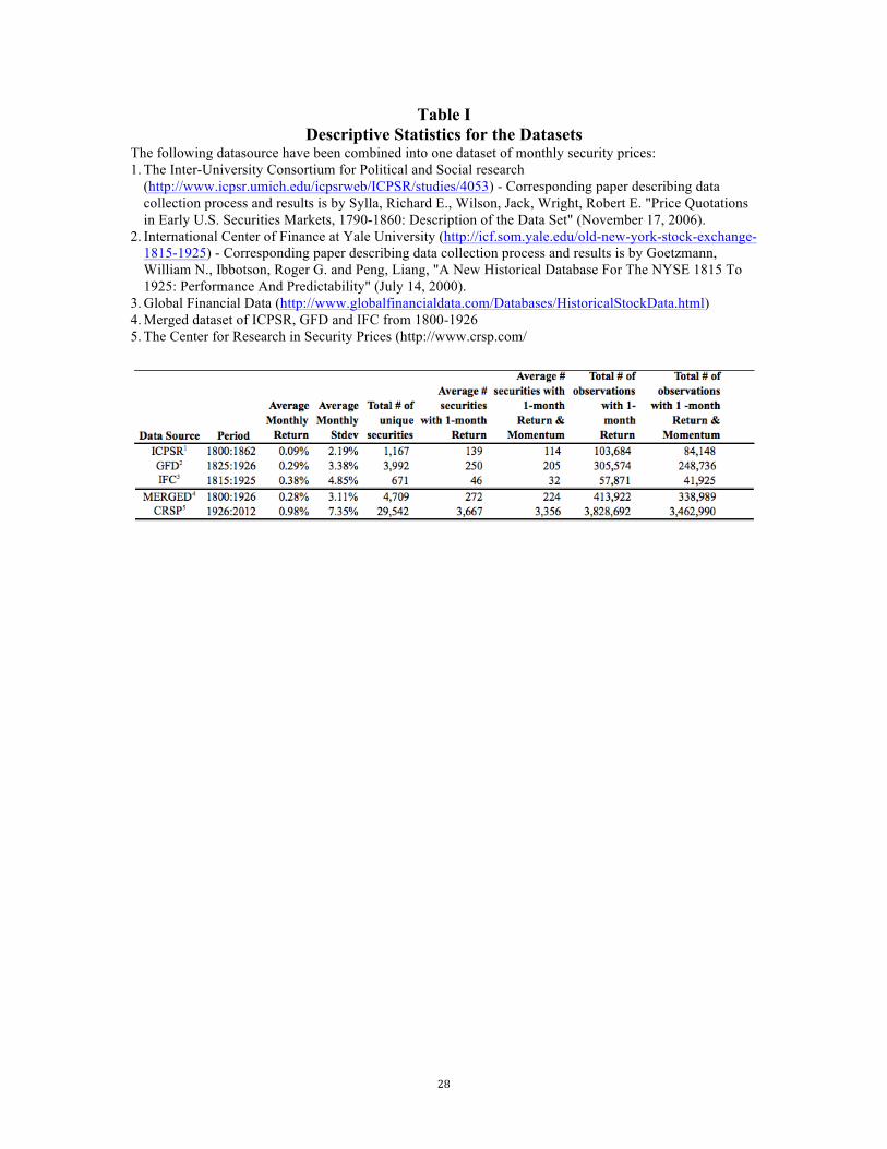
Global Financial Data (GFD) – [Table I].

ICF dataset was created for and described in detail in “A New Historical Database

for the NYSE 1815 to 1925: Performance and Predictability” (Goetzmann, Ibbotson,

Peng (2000)). A total of 671 NYSE stocks are covered between January 1815 and

                                                                                                               1  According  to  William  Goetzman,  email  correspondence.    

   

    6  

December 1925. Month-end equity prices were manually collected at a monthly

frequency from archived newspapers of the time. A total of 57,871 unique month-return

observations occur.

ICPSR dataset was created for “Price Quotations in Early United States Securities

Markets, 1790-1860” (Sylla, Wilson, Wright (2002)). We filter out any preferred, fixed

income, or international securities resulting in a total of 1167 common U.S. stocks

covered between January 1800 and May 1862. Prices were manually collected from

archived newspapers of the time for nine U.S. exchanges: New York, Boston,

Philadelphia, Baltimore, Charlestown, New Orleans, Richmond, Norfolk, and

Alexandria. Within any given month, price frequency ranges from daily to monthly. To

convert ICPSR data to a monthly frequency, we allow for a look-back window of one

month minus a day. Hence, if a security price is missing during the month-end date, we

look back for the last available price during the same calendar month. This significantly

improves data coverage for stocks whose prices are available only in the weeks not

coinciding with month-end. Sometimes an ask price would be supplied in addition to the

bid price, in which case we would average the two. As a result, a total of 103,684 unique

month-return observations are recorded.

GFD dataset was acquired for this study from Global Financial Data. There are

3992 common stocks covered in the dataset between January 1825 and December 1926.

Due to the reporting format of the newspapers used for this data collection, month-end

prices represent averages of the maximum and minimum prices reached during each

calendar month. A total of 305,574 unique month-return observations are noted.

   

    7  

We merge the three datasets creating the Merged dataset by using company names

and correlation of prices, since there is no other common security identifier between the

three datasets. Naming conventions between the three datasets vary greatly in terms of

abbreviations, articles, order of words etc., so a simple name comparison without price

correlations is not sufficient. Since GFD database is the largest, we use all available GFD

data as a starting point and supplement it with unique data from ICF and ICPSR sources.

We follow the following procedure. First, for each ICF security, a list of GFD securities

is generated with which they have the highest price correlation. Next, a manual

comparison of ICF’s security name and the names in the generated list is conducted, and

if there is a clear match of names, they are paired; otherwise, ICF security is labeled as

unique. Then the same procedure is done for the ICPSR securities against the merged

GFD and ICF dataset. All ICPSR securities are assigned to a list labeled ‘unique’ or

‘already included’ in the GFD-ICF dataset.

We identify 222 unique securities in the ICF and an additional 401 unique

securities in ICPSR datasets that were additive to the GFD dataset, resulting in a total of

4709 unique securities in the merged dataset. Importantly, in addition to forming a larger

set of unique securities, Merged dataset fills in missing data for the GFD individual

securities, creating a richer dataset. A missing month-end price for a security in the GFD

dataset is searched for in the other two sources, and is plugged in if it is available. The

merged dataset also results in an extended coverage period from January 1800 to

December 1926. The only interruption of the Merged data is during the two first months

of World War I in 1914. A total of 413,922 unique month-return observations appear in

the merged dataset.

   

    8  

The number of securities with monthly return data grows from 10 on January

1800 to 781 on December 1926. For the majority of the period, the number of securities

grows steadily, with the exception of the Civil War period in the early 1860s, when a

large drop in coverage takes place. This drop is witnessed by Goetzmann et al. and is due

to newspapers dropping coverage of many traded securities. After reaching a maximum

of 415 securities in July 1853, the number first slowly and then rapidly drops to a

minimum of 53 in January 1866. From then on it slowly grows back up, crossing 400 in

May 1899.

To compute the universe returns we use the equally weighted method of price

only returns, because we do not have reliable shares outstanding or dividend information.

Dividend data that accompanies the ICF dataset is available only annually from 1826 to

1871 for 255 companies. ICPSR does not provide dividend data and GFD is still in the

process of gathering that information. This makes any attempt to compute total returns

for individual securities and the momentum effect impossible at this stage. We believe

that price returns are sufficiently accurate for the purposes of extending the price

momentum studies, as an assumption is made that the dividends on the Winners roughly

offset the dividends of the Losers.

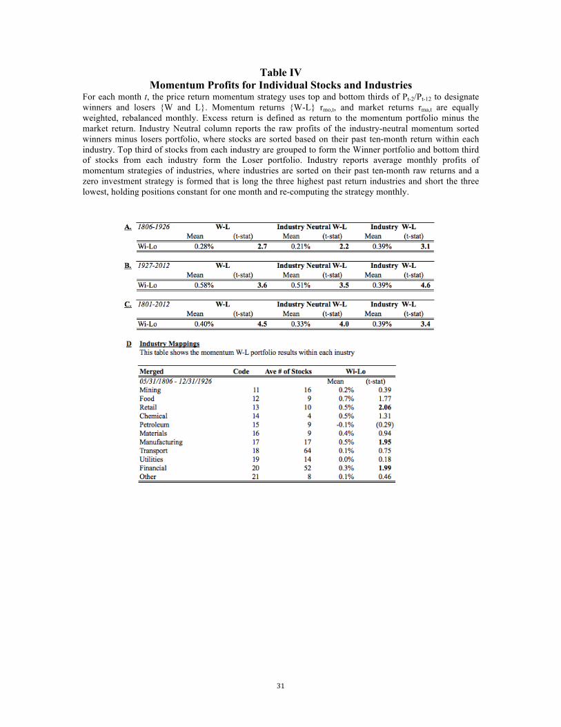
Industry mappings for the merged dataset are derived from the industry

assignments in the individual datasets and aggregated to the level that was both granular

enough to capture industry differences, while maintaining a large enough number of

firms in each group. From 52 GFD Industries, 6 IFC Sectors and 4 ICPST sectors, 11

final industry groupings are derived: Mining, Food, Retail, Chemical, Petroleum,

Materials, Manufacturing, Transportation, Utilities, Financial, and Other. Smallest sector

   

    9  

is Chemical with an average of 4 stocks over the period. The largest is Transportation

with an average of 69 stocks. Industry data is available from the beginning of the dataset,

but the concentration is high in financial companies. Over the course of the 19th century,

more industries begin to emerge, reaching a required level of three by 1806, a figure

necessary for the industry momentum computation. Industry mappings in this study are

used to estimate industry-neutral and industry-level momentum.

For the post-1927 period, the Center for Research in Security Prices (CRSP) is

relied on for its database of security prices. The same market and momentum return

computation methodology is applied to the CRSP data as it is to the Merged data in order

to preserve consistency of results. Additionally, we download the macro-economic data

from Global Financial Data and Measuring Worth websites2.

II. The Price Momentum Anomaly

A. Background

Out-of-sample record of momentum has been exceptional. The positive premium

has continued after its published discovery in the U.S. market (Jegadeesh, Titman (1993)),

in the international markets (Rouwenhorst (1997)), aggregate market indices (Asness,

Liew, Stevens (1997)), currencies (Bhojraj, Swaminathan (2006)), and commodities

(Gorton, Hayashi, Rouwenhorst (2012)). A recently updated study of “Momentum

Everywhere” traces the power of the anomaly across the globe (Asness, Moskowitz,

Pedersen (2008)). The momentum effect is also confirmed in the 19th century British

stock prices (Chabot, Ghysels, Jagannathan (CGJ 2009)).

                                                                                                               2  www.measuringworth.com  

   

    10  

Since the discovery of the momentum anomaly (JT 1993), a large body of

research attempts to isolate a risk-based explanation for the effect, inline with market

efficiency. The following studies provide the theoretical roadmap for our discussion:

Moskowitz, Grinblatt, (MG 1999); Grundy, Martin (GM 2001); Chordia, Shivakumar

(CS 2002), Griffin, Ji, Martin (GJM 2003); Cooper, Gutierrez, Hameed (CGH 2004),

Siganos, Chelley-Steeley, (SCS 2006), Liu, Lu (LL 2008), Asem, Tian (AT 2010),

Stivers, Sun (SS 2012).

These studies investigate whether momentum profits are driven by industry

effects (MG 1999); variation of expected returns (GM 2001); factor-level versus stock-

specific momentum (GM 2001); macroeconomic factors (CS 2002, GJM 2003, LL 2008);

or market states (CGH 2004, SCS 2006, SS 2012). The later studies agree that industry

momentum is a separate effect from stock-level momentum and find that market state is a

better proxy for risk than macro-economic variables.

By far, the most insightful observation by JT (1993) and more formally by GM

(2001) explores the connection between momentum portfolio beta loading and the factor

realization over the portfolio formation period. GM (2001) proves analytically and

demonstrates empirically that momentum portfolio is loaded with high beta stocks during

the bull market and negative beta stocks during the bear market.

This has led to a growing number of studies studying the connection between

market states and momentum profits. CGH (2004) observes that momentum returns

following an up market are higher than following the down market. SCS (2006) find that

momentum profits are stronger after lagging poor market returns, where the longer the

duration to describe the poor market, the stronger the momentum returns realized.

   

    11  

Finally, AT (2012) and SS (2012) observe that momentum returns are stronger within a

given state and are weaker during state transitions.

This study further explores the connection between market states and momentum

via the dynamic relationship between momentum beta and the market state duration.

Adding a duration concept to the market state definition allows us to track evolution of

momentum beta and alpha both across and within market states. We find that state

duration critically determines the factor loading of the momentum portfolio, which in

turn affects the size and direction of momentum profits within and across market states.

B. Empirical Results

Momentum is defined as the stock’s price change from t – 12 to t – 2, skipping the

reversal effect. Every month in the research sample, each stock each stock is assigned to

one of three portfolios based on prior 10-month price change. Stocks with the highest

momentum are assigned to the Winner (W) portfolio, and stocks with the lowest

momentum are assigned to the Loser (L) portfolio. The portfolios are re-balanced

monthly, and one-month forward equally weighted return of each portfolio is computed.

Excess returns are derived by subtracting average return of all stocks form the

momentum portfolio return. Returns to this strategy are observed between February 28,

1801 and December 31, 2012.

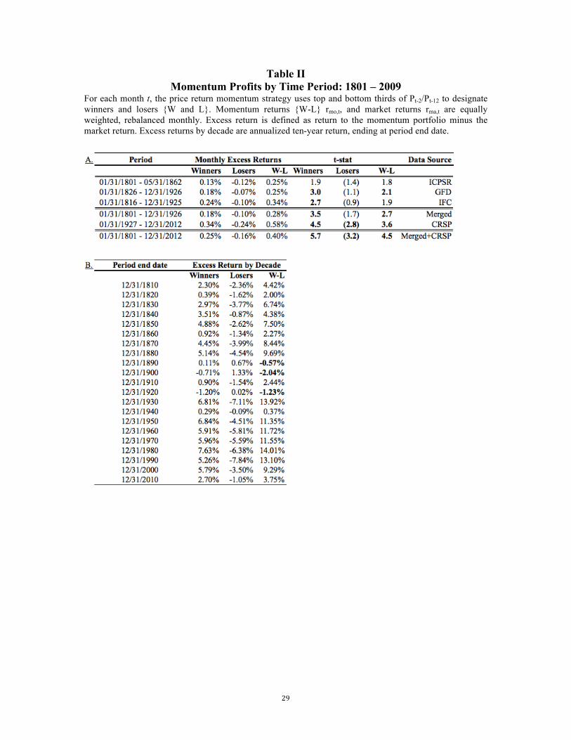
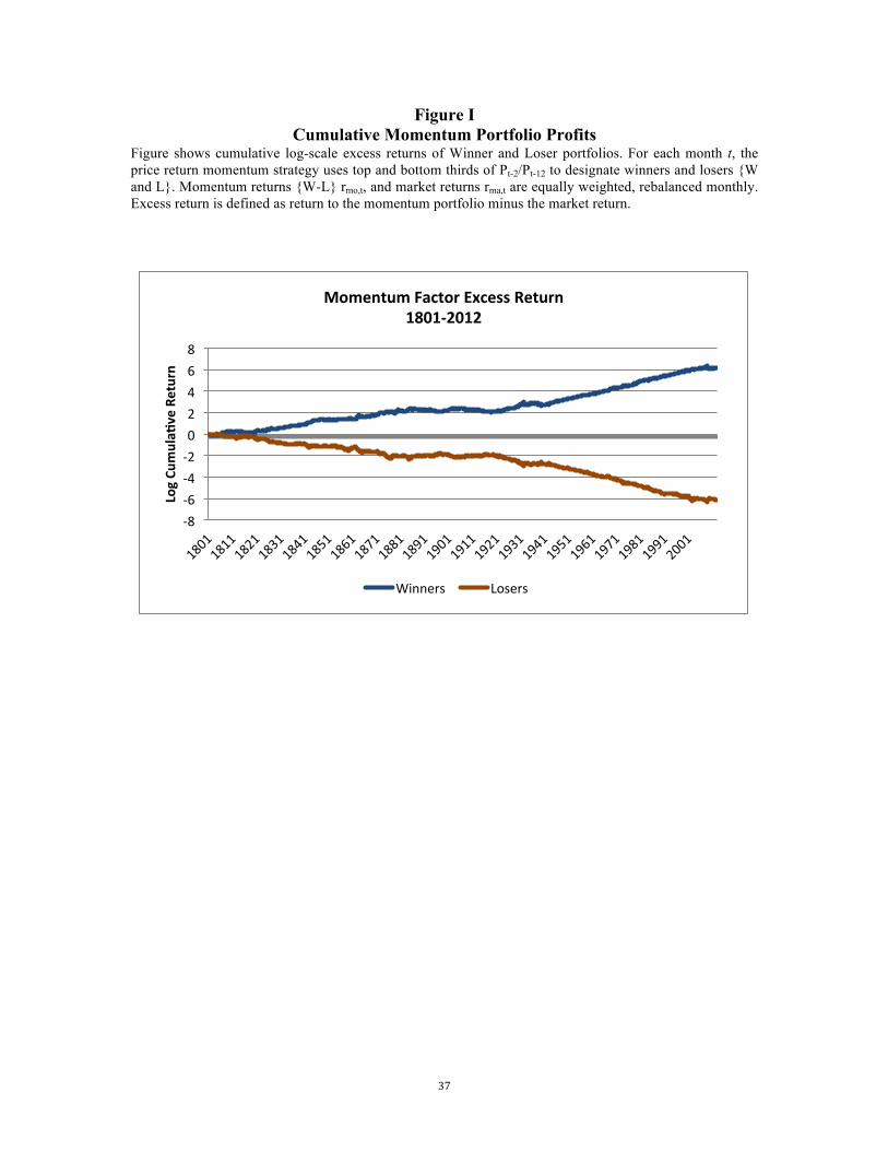
During the 1801-1926 period, the average monthly excess return of the W

portfolio is 0.18% (t-stat 3.5), the L portfolio is -0.10% (t-stat 1.7), and the W-L portfolio

is 0.28% (t-stat 2.7). During the 1927-2012 period, the W portfolio average monthly

excess return is 0.34% (t-stat 4.5), L portfolio -0.24% (t-stat 2.8), and the W-L return is

   

    12  

0.58% (t-stat 3.6). During the entire period from 1801-2012, W-L return is 0.40% (t-stat

4.5); W portfolio excess return is 0.25% (t-stat 5.7) and L portfolio excess return is -

0.16% (t-stat 3.2). – [Table II, Figure I].

The previously untested pre-1927 data confirms the significance of the

momentum anomaly in the 19th and early 20th century U.S. stocks. The combined history

creates the longest known U.S. stock-level backtest of 212 years (or 2543 months of

momentum observations). The size of the anomaly is stronger in the post-1927 period,

yet it remains significant in both sub-periods. We observe positive W-L momentum

returns in individual pre-1927 datasets as well. Using ICPSR data only, the W-L spread is

0.25% per month (t-stat 1.8) for the 1801-1862 period; using GFD data only, W-L spread

is 0.25% (t-stat 2.1) for the 1826-1926 period; and IFC data W-L spread is 0.34% (t-stat

1.9) for 1816-1925 period. The momentum effect is present in each of the three very

differently assembled datasets.

The overlapping period across the three datasets is from 1826 to 1862. In this

period the W-L monthly spreads are: ICPSR +0.17%, GFD +0.38%, and ICF +0.44%.

The merged dataset over this period generates 0.33% W-L spread. The overlapping

period reveals the increased robustness effect achieved by merging the three datasets.

Between 1826 and 1862, ICPSR has a monthly average of 158 securities with return data,

GFD has 107 such securities, and ICF has 15. The merged dataset results in the monthly

average of 212 testable securities, with about 71 stocks in the W and L portfolios. As

expected, the greatest synergy between the datasets occurs during this overlapping

period, which is when such synergy is most effective because of the generally lower

quality of data in the early and mid 19th century.

   

    13  

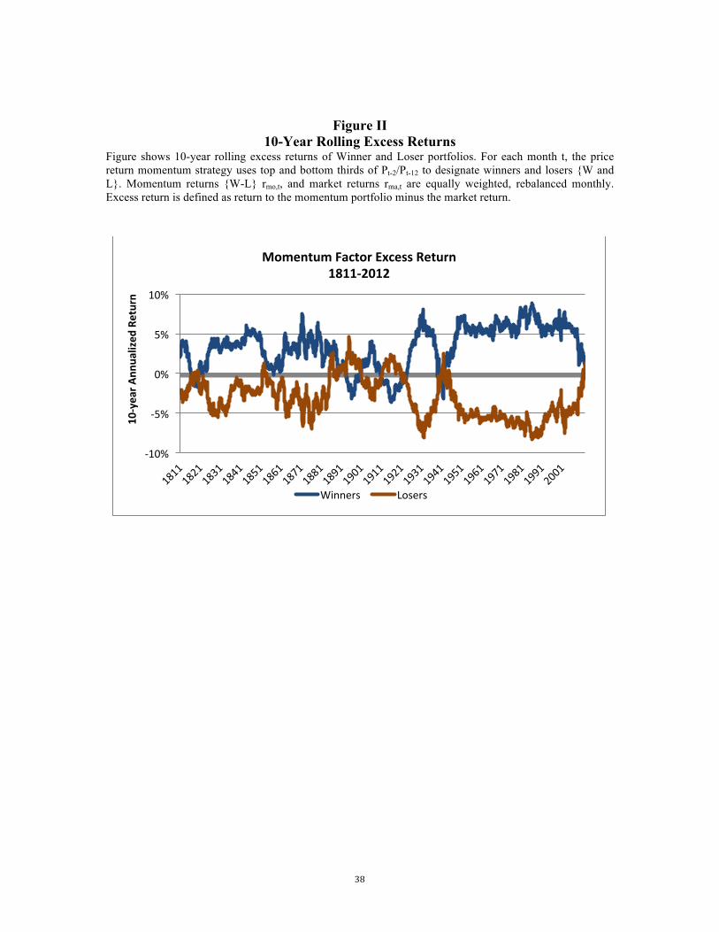
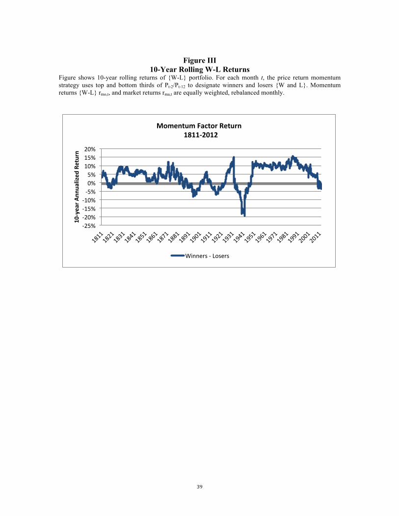
As observed by GM (2001), CGJ (2009), significant time variation to momentum

payoffs occurs. Table II.B shows the annualized return of momentum portfolios by

decade. During the pre-CRSP history, 10-year annualized return is negative in three

decades (1890: -0.6%, 1900: -2.1%, and 1920: -1.2%). On a 10-year rolling basis, there

are seven negative periods. [Figure III]. These are significant 10-year drawdowns that

support CGJ (2009) limits to the arbitrage explanation of momentum profits. Any levered

investor in the momentum strategy would have experienced a margin call during these

periods. During the rest of the early history, 10-year profitability varied between 0% and

15.3% per year.

During the recent decade of negative momentum performance (from

January’2002 to December’2012) the annualized W-L spread of is -2.1%, which is

consistent within a longer historical timeframe. The pre-1927 data captures a more

complete distribution of momentum profits than what has been observed since 1927.

Even though extended history by itself does not prove or disprove whether momentum

effect has been arbitraged out by the large amount of capital deployed into this strategy

over the last two decades, it does provide evidence that such periods of extended

underperformance have occurred in the past. Limits to the arbitrage hypothesis, stating

that momentum profits are too risky to be fully arbitraged, would suggest that the latest

period of under-performance would eventually give way to positive momentum returns

once again.

The January effect is in the same negative direction before 1927 as it is after. In

the 1801-1926 period, average W-L spread during the month of January is -0.1%, while it

is 0.3% during non-January months, although the January t-statistic is not significant (t-

   

    14  

stat 0.32) during the early period. Post-1927 period W-L January return is -3.3% (t-stat

6.0) and non-January spread is 0.9% (t-stat 7.2) - [Table V]. Because the January return is

negative in both periods, longer history does imply that the effect is less likely to be a

random aspect of 20th century data.

We observe a similar term-structure of momentum profits after the formation

month in the pre-1927 as in the post-1927 era - [Table III]. On average, between 1801

and 1926, momentum profits continue to accumulate up to the fourth month after

portfolio formation, and up to the fifth month in post-1927 period. Returns are

statistically significant for the first and second months in both periods.

Confirming existing long-term reversal studies (DeBondt and Thaler (1985), JT

(1995)), momentum profits experience a significant reversal after eight months from

portfolio formation. The power of mean reversion is strong, as we are measuring non-

overlapping future one-month performance of the W-L strategy. So, for example, in

month 11 after portfolio formation, the W-L return in the pre-1927 period is -0.31% with

a t-stat of 3.1, and in the post-1927 period, it is -0.78% with a t-stat of 5.8. The negative

returns persist for up to five years after portfolio formation.

III. Sources of Momentum Profits

A. Industry-Neutral Momentum

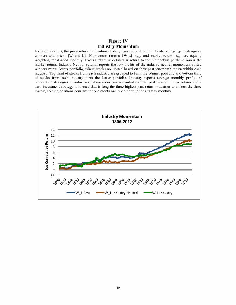
We first examine if industry momentum explains stock level momentum and find

that it does not. However, as in the post-1927 period, industry momentum is a separate

and significant effect in the pre-1927 data. Using the constructed industry classifications

   

    15  

we test an industry-neutral momentum portfolio by ranking each stock within its industry

on its 10-month price change. We then combine the top third ranked stocks from each

industry into a Winner portfolio and the bottom third into a Loser portfolio. Rebalancing

monthly, we find that between 1801 and 1927 the industry-neutral average monthly W-L

return is 0.21% (t-stat 2.2), compared to the raw 0.28% (t-stat 2.7) - [Table IV]. We then

construct an industry momentum portfolio by identifying the three industries out of the

ten with the highest and three with the lowest 10-month trailing returns (skipping the

reversal months). The resulting W-L return of the monthly rebalanced industry portfolio

is 0.4% (t-stat 3.1). For the full history between 1801 and 2012, industry momentum

spread is 0.39% (t-stat 3.4) and industry-neutral momentum is 0.33% (t-stat 4.0).

Consistent with GM (2001) and many others, pre-1927 data confirms that

industries have a momentum of their own, which does not explain away the stock level

momentum - [Figure IV].

B. Common vs. Stock-Specific Momentum

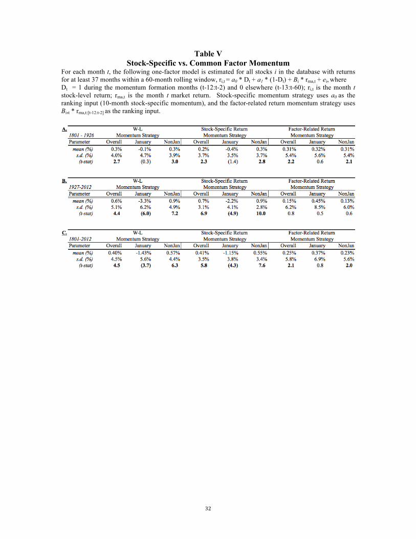
Following the GM (2001) methodology, we test whether the stock-specific

momentum is the significant driver of the W-L portfolio. Using a 60-month rolling

regression (requiring a minimum of 37 months of data), we decompose momentum

returns into stock-specific momentum and factor momentum by regressing stock return

on a dummy variable and the market return

ri,t = a0 * Dt + a1 * (1-Dt) + Bi * rma,t + ei, (1)

where Dt = 1 during the momentum formation months (t-12:t-2) and 0 elsewhere (t-13:t-

60); ri,t is the month t stock-level return; rma,t is the month t market return. Stock-specific

   

    16  

momentum strategy uses a0 as the ranking input (10-month stock-specific momentum),

and the factor-related return momentum strategy uses Bi,t * rma,t:[t-12:t-2] as the ranking

input - [Table V]. Confirming GM (2001), we find that stock-specific momentum is

positive and significant. Between 1801 and 1927, the average stock-specific W-L

portfolio spread is 0.22% per month (t-stat 2.3), and for the 1927-2012 period it is 0.7%

per month (t-stat- 6.9).

The common factor momentum component is also positive in both periods. For

the entire period, the common factor momentum spread is 0.25% (t-stat 2.1). The

common factor momentum is more significant in the early history with a spread of 0.31%

(t-stat 2.2). Importantly, the longer history makes it clear that both the stock-specific and

common factor momentum are priced. As our further results will demonstrate, the pricing

of these factors occurs at different points of a given market state with the stock-specific

momentum payoff more dominant at the early stages of a market state, while the

common-factor component more dominant at later stages.

C. Beta Variation of Momentum Portfolios

Many studies argue that market states are a better proxy for macro economic

variables, as the market is seen as a timelier leading indicator3. We concur with this

observation and suggest that because momentum factor becomes riskier the longer a

market-state lasts, when the economic conditions change, the strong beta exposure at the

                                                                                                               3  Unreported  in  this  paper,  we test whether common macro-economic indicators explain momentum profits and concur

with CGH (2003) that no single macro economic variable explains momentum profits. We test change in expected inflation (DEI); unexpected inflation (UI); term-premium (UTS); growth of industrial production (YP); default-premium (URP); consumption growth (CG); where CG is proxied by wage growth; commodity price growth (CG); FX $ versus pound exchange (FX); and residual market (RES) computed by regressing the macro variables from the market return and using the residual as a factor. Only the UTS factor is found to be significant in the post-1927 period.  

   

    17  

worst possible time significantly harms momentum profits. In our view, one of the most

significant contributions of GM (2001) is the analytical proof and empirical

demonstration of the variation of momentum beta exposure as a function of the trailing

market return. When the market has been positive during the momentum formation

period, momentum portfolio’s beta is positive, and negative following negative market

return. Even though obvious, it is often a misunderstood dynamic risk property of the

momentum portfolios. The recent observation of this risk occurred in 2009 when the

momentum beta loading was negative and the market experienced a strong rally.

Because market state and momentum definitions vary across studies, the results

are difficult to compare. For example, GM (2001) defines up and down states as the 6-

month trailing equally weighted total return of the market above / below one standard

deviation around the full sample average return. In contrast, CGH (2004) defines market

states as the sign of the 36-month trailing value weighted total return of the CRSP index.

Finally, SS (2012) defines market states based on a peak to trough ex-post value

weighted total return in excess of +/- 15%. While CGH (2004) conclude that momentum

returns are positive only following the up markets, SS (2012) conclude that momentum

returns are positive within a given market state, either up or down, and negative during

transitions.

We use a market state definition that matches the momentum portfolio formation

definition. Momentum formation period covers 10 trailing months (skipping the reversal

months), and the market state definition uses the same 10 months. Instead of making the

trailing periods longer, and as a result misaligning the formation periods, we can use state

duration variable to describe the length of a market state. Our comprehensive definition

   

    18  

of a market state has two parts: the sign of the market return during momentum portfolio

formation, and the number of consecutive months of that market return sign (duration

variable). The first part aligns market state with the momentum portfolio, while the

second captures the concept of state duration. Hence, in this study market state is defined

as an equally weighted, price only return of the market over the momentum formation

period (t-12:t-2) and a duration variable that measures the number of consecutive months

in a given state.

We first construct a one-factor version of GM (2001) test adapted to our

definition of momentum portfolio and market states, estimating the following two

regressions:

rmo,t = amo + Bmo * Dt *rma,t + emo,t (2)

and

rmo,t = amo + BmoDOWN*DtDOWN*rma,t + BmoUP*DtUP rma,t + emo,t, (3)

where dummy variable Dt {down, up} is: 1 if the cumulative performance of the Market

over months t-12 to t-2, is {negative, positive}.

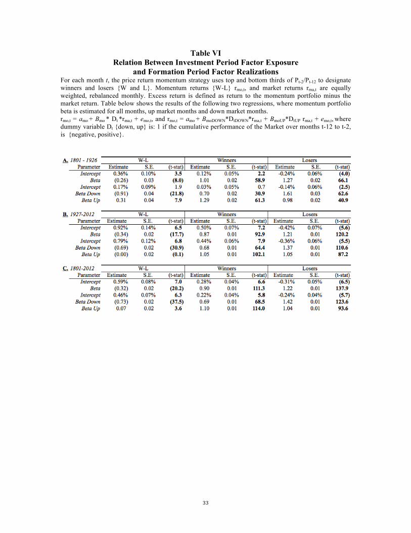
We confirm that before 1927, average beta of momentum W-L portfolio is

negative (-0.26, t-stat -8.0), while the alphas are significantly positive 0.36% (t-stat 3.5) -

[Table VI]. We also confirm that in an up market, momentum beta is positive (0.31 t-stat

7.9) and in the down market it is negative (-0.91 t-stat 21.9). For the 1927-2012 period,

average W-L beta is -0.34 (t-stat 17.7). The magnitude of the beta variation is about twice

as large in the pre-1927 period as in the post-1927. For the entire period 1801-2012, W-L

momentum beta is -0.32 (t-stat 20.2).

   

    19  

In the pre-1927 period, negative beta is a result of the L portfolio average beta of

1.27 vs. the W portfolio average beta of 1.01. In the down markets, W portfolio beta

drops to 0.7 and L beta rises to 1.6. Reverse occurs in the up markets with W portfolio

beta rises to 1.3 and L beta drops to 0.98. Since the level of beta in the momentum

portfolio is analytically linked to recent market performance, it is not a surprise to find

similar results as GM (2001) in the pre-CRSP data. Nevertheless, it is fascinating how

powerful the beta variation of a momentum portfolio is.

More importantly, studies that document connections between market states and

momentum performance could be explained by first observing the beta of the momentum

portfolio within a market state, because it is the beta exposure that causes raw momentum

profits to correlate with market states. Depending on the definition of the market state,

the observed correlations between momentum and market states will be different, but the

cause of the correlation is the beta of the stocks inside the momentum portfolios, and

hence once measured, the momentum portfolio beta can explain the direction of market

state correlation with momentum profits.

We further investigate this connection between market state and momentum beta

exposure by focusing on the duration of the realized market state and its effect on the

momentum portfolio beta exposure. We find strong evidence that momentum beta is

dynamic not only across up and down market states but also within a given market state.

Momentum beta is positively exposed to the duration of both positive and negative states.

The longer each state persists, the stronger the beta becomes.

A state duration variable is created by summing the number of consecutive

positive / negative market states until the state changes. This variable provides additional

   

    20  

visibility into momentum portfolio dynamic over the course of a market state. We

compute the exposure of momentum beta to market state duration in the following way:

First, a 10-month rolling momentum beta is obtained by regressing monthly momentum

returns (rmo,t) on a constant and equally weighted market return (rma,t).

rmo,t = amo + Bmo *rma,t + emo,t. (5)

Next, calculated Bmo,t are regressed on the market state duration variable:

Bmo,t = ab + Coefb* Durationt + eb,t, (6)

where Duration is the length of the consecutive months in a given state. Duration is

positive during the up market states and negative during down market sates. For example,

if the market state has been positive for two months in a row, duration is set to two.

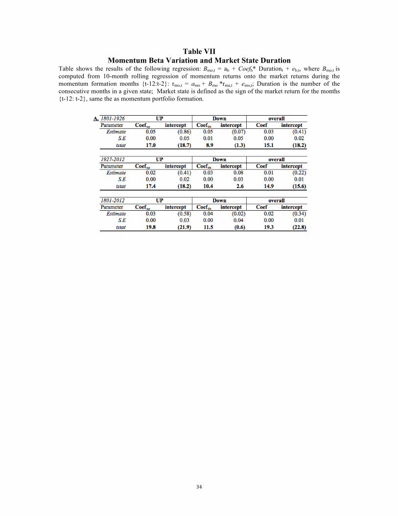
In this explanatory model, we find a strong dependence between momentum beta

and market state duration. Full period coefficient is 0.02 (t-stat 19.3). Up state coefficient

is 0.03 (t-stat 19.8), and down state coefficient is 0.04 (t-stat 11.5). Hence, the higher the

market state duration variable, the stronger the momentum portfolio beta becomes -

[Table VII, Figure V]. In the pre-1927 period, the up state coefficient is 0.05 (t-stat 17.0)

vs. the post-1927 period up state coefficient of 0.02 (t-stat 17.4). The pre-1927 down

coefficient is 0.05 (t-stat 8.9) and post-1927 period down coefficient is 0.03 (t-stat 10.4).

This confirms prior observations that momentum beta variability is higher in the pre-1927

period.

Duration variable helps refine GM (2001), who only capture the average betas

following up and down market states. Our study shows that only after the market state

has been occurring for some time does momentum beta actually take on those signs, and

   

    21  

that in the beginning of each state, momentum beta is actually opposite form the new

market direction.

D. Alpha and Beta Contribution

The dynamic nature of beta over the course of a market state provides the

following insights. In the first year of a new market state, momentum beta will be

opposite from the market direction, hence generating a negative drag on momentum

performance. During the first year of a market state, momentum portfolio starts by being

long last state’s winners and short last state’s losers, which have the opposite beta tilt

from the new market direction. In the second year and beyond, momentum beta takes on

the sign of the market direction and begins to add to momentum returns. The longer a

market state persists, the higher the beta and the more such exposure contributes to the

momentum portfolio return. This effect explains why both the stock specific and factor

momentum components are priced. It also explains why momentum underperforms after

market reverses direction.

To measure this effect, we look at the average alpha and beta components of

momentum portfolio return as a function of the market state duration - [Table VIII,

Figure VI]. For every month t, we calculate momentum alpha as the difference between

raw momentum return and the CAPM 10-month rolling beta multiplied by the market

return for that month. The beta contribution is derived by subtracting the alpha

contribution from momentum raw returns. Our results show a striking evolution of the

source of momentum profits over the course of a market state.

   

    22  

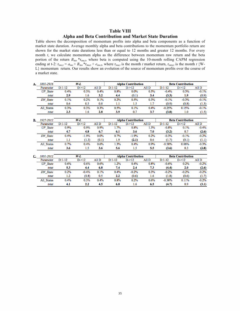
In the overall history, average monthly momentum returns within the first year of

all market states is 0.4% (t-stat 4.1) vs. 0.3% (t-stat 2.2) in the subsequent market state

months. Beta contribution is -0.4% (t-stat 4.7) in the first year, and +0.1% (t-stat 0.1) in

the subsequent market state months. Alpha contribution is significantly positive in the

first year (0.8%, t-stat 6.8) and positive but not significant in the subsequent months

(0.2%, t-stat 1.6). As market state continues and momentum portfolio beta changes with

market direction, the contribution from the beta component switches from significantly

negative to slightly positive, while the alpha portion declines from significantly positive

to insignificantly positive. As a result, momentum return increases with state duration,

but there is also an increase in systematic risk via a combination of increasing beta and

the conditional probability of state upcoming reversal.

Breaking down the sample into up and down market states, a similar pattern can

be seen. For example, alpha contribution in first 12 months of an up state is 1.2%, while

the beta contribution is -.6%. In the subsequent months of an up state, alpha contribution

declines to 0.4% while beta contribution rises to 0.2%. In the down markets, during the

first 12 months, alpha contributes 0.4%, while beta contributes -0.2%. In the subsequent

months, alpha contribution drops to -0.2%, while beta contribution remains at -0.2%.

The reason that the beta contribution in the first 12 months vs. subsequent months

is asymmetric between up and down states is because the momentum beta at the end of a

average down state is -0.34 (t-stat 3.5), while it is insignificant 0.02 (t-stat 0.2) at the end

of the average up state. This occurs because the volatility of the down states is larger

leading to large absolute beta. Therefore, the expected average beta following the average

down markets is highly negative, while following average duration up markets it is

   

    23  

insignificant from 0. This is the reason why the first 12 months of a new up state

experience a large negative beta contribution, while the first 12 months of a down state

do not.

Our findings provide the support for SS (2012) argument that momentum is

higher within a state, than across states. This is due to the dynamic nature of

momentum’s beta. When a new state starts, the duration variable resets to zero, and the

beta of the momentum portfolio starts a new cycle of adjusting to the new state. During

this adjustment period of one year, beta’s negative contribution to momentum portfolio

makes returns during state transitions lower than during state continuations.

Our findings support CGH (2004) that momentum returns are stronger following

the positive market states than negative. However, we point out that this occurs mainly

due to the negative market states that last longer than a year. Momentum experiences

significant negative returns due to the negative beta exposure caused by lasting bear

markets such as 1930’s and 2000’s. In market states under one year, momentum profits

remain positive.

E. Dynamically Hedged strategy

To account for the dynamic variation of momentum’s beta, we test the following

feasible ex-ante hedging strategy. If the market state has just changed, we hedge out the

beta exposure of the momentum portfolio for the first 10 months of the new up market

state and the first 7 months of the new down state – accounting for the beta asymmetry

between up and down states. At month 10 for up and month 7 for down, the hedge is

turned off, and we allow for the beta contribution to add to momentum returns.

   

    24  

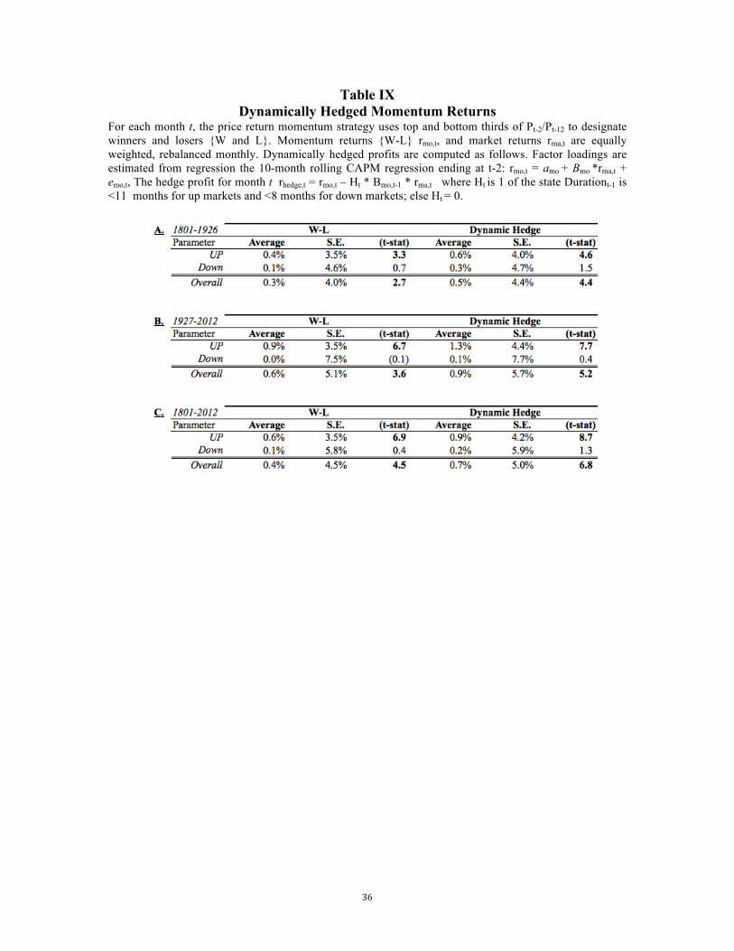
During the full sample, the dynamically hedged strategy generates a large increase

in performance in the up states from 0.6% per month (t-stat 6.9) to 0.9% per month (t-stat

8.7), and in the down states, from 0.1% (t-stat 0.4) per month to 0.2% per month (t-stat

1.3) - [Table IX]. Between 1801 and 2012, the average monthly dynamically hedged

Long Short return increases to 0.7% (t-stat 6.8) from the raw momentum return of 0.4%

(t-stat 4.5). Figure VII plots the cumulative returns to the hedged and the raw momentum

strategy. Of practical significance to investors utilizing momentum signals, is the fact that

the hedged momentum strategy significantly outperforms raw momentum strategy during

the periods with large market reversals such as the last ten years.

IV. Conclusion

We initiate out-of-sample research of the 19th and early 20th century stock-level

data by identifying three datasets that can be used for such studies, and creating a merged

dataset that combines all three. Test of the price momentum strategy is extended to the

new data and its effect is found to be significant since the beginning of the 19th century.

Using the longer time-series, a robust connection is observed between momentum

portfolio beta, alpha and the duration of up and down market states. The longer each state

continues, the higher the proportion that the beta exposure contributes to momentum

returns. Therefore, the momentum factor becomes riskier the longer a market state lasts,

and when the economic conditions change, the strong beta exposure significantly harms

momentum profits. Dynamically hedging out beta in the early stages of a market state

significantly improves the profitability of momentum strategy.

   

    25  

References Asem, Ebenezer, and Gloria Tian, 2010, Market dynamics and momentum profits,

Journal of Financial and Quantitative Analysis 45, 1549–1562. Asness, Clifford S., Moskowitz, Tobias J., and Pedersen, Lasse Heje, 2009, Value and

Momentum Everywhere, AFA 2010 Atlanta Meetings Paper. Asness, Cliff S., Liew, John, M., and Stevens, Ross L., 1997, Parallels Between the

Cross-Sectional Predictability of Stock and Country Returns, The Journal of Portfolio Management 23, 79-87.

Bhojraj, Sanjeev, and Swaminathan, Bhaskaran, 2006, Macromomentum: Returns

Predictability in International Equity Indices, The Journal of Business 79, 429–451. Campbell, John Y., and Vuolteenaho, Tuomo, 2004, Bad beta, good beta, American

Economic Review 94, 1249–1275. Carhart, Mark. M., 1997, On persistence in mutual fund performance, Journal of Finance

52, 57–82. Chordia, Tarun, and Shivakumar, Lakshmanan, 2002, Momentum, business cycle, and

time varying expected returns, The Journal of Finance 57, 985–1019. Cooper, Michael, Gutierrez, Roberto, and Hameed, Allaudeen, 2004, Market states and

momentum, The Journal of Finance 59, 1345–1365. Chabot, Benjamin, Eric, Ghysels, and Jagannathan, Ravi, 2009, Price Momentum in

Stocks: Insights from Victorian Age Data, NBER working Paper No. w14500. Chan, Louis K. C., Jegadeesh, Narasimhan, and Lakonishok, Josef, 1996, Momentum

strategies, Journal of Finance 51, 1681–1713. Chen, Nai-Fu, Roll, Richard, and Ross, Stephen, A., 1986, Economic forces and the stock

market, Journal of Business 59, 383-403. Cole, Arthur, H., and Frickey, Edwin, 1928, The Course of Stock Prices, 1825-66,

Review of Economics Statistics 10, 117-139. Conrad, Jennifer, and Kaul, Gautam, 1998, An anatomy of trading strategies, Review of

Financial Studies 11, 489 - 519. Cowles, Alfred, 1939, Common Stock Indices, Principia Press, Bloomington. DeBondt, Werner F.M., and Thaler, Richard H., 1985, Does the stock market overreact,

Journal of Finance 40, 793-805.

   

    26  

Fama, Eugene, and French, Kenneth, 1989, Business conditions and expected returns on

stocks and bonds, Journal of Financial Economics 25, 23–49.

_______,1996, Multifactor explanations of asset pricing anomalies, The Journal of Finance 51,

55–84.

_______, 2008, Dissecting anomalies, The Journal of Finance 63, 1653–1678. Goetzmann, William, Ibbotson, Roger, G., and Peng, Liang, 2001, A New Historical

Database for the NYSE 1815 to 1925: Performance and Predictability, Journal of Financial Markets 4,1–32.

Gorton, Gary B., Fumio Hayashi, and Rouwenhorst, Geert, K., 2012, The Fundamentals

of Commodity Futures Returns, Yale ICF, working paper 07-08. Griffin, John, M., Ji, Susan, and Martin, Spencer, J., 2003, Momentum investing and

business cycle risks: Evidence from pole to pole, The Journal of Finance 58, 2515–2547.

Grundy, Bruce, and Martin, Spencer, J., 2001, Understanding the nature of the risks and

the source of the rewards to momentum investing, The Review of Financial Studies 14, 29–78.

Jegadeesh, Narasimhan, and Titman, Sheridan, 1993, Returns to buying winners and

selling losers: Implications for stock market efficiency, The Journal of Finance 48, 65–91.

_______, 1995, Overreaction, delayed reaction, and contrarian profits, Review of

Financial Studies 8, 973 - 993. _______, 2001, Profitability of momentum strategies: An evaluation of alternative

explanations, The Journal of Finance 56, 699–720. Kang, Qiang and Li, Canlin, 2004, Understanding the Sources of Momentum Profits:

Stock-Specific Component versus Common-Factor Component, EFA 2004 Maastricht Meetings Paper No. 3629.

Lakonishok, Josef, Shleifer, Andrei, and Vishny, Robert, W., 1994, Contrarian

investment, extrapolation, and risk, Journal of Finance 49, 1541–1578. Liu, Laura, and Zhang, Lu, 2008, Momentum profits, factor pricing, and macroeconomic

risk, The Review of Financial Studies 21, 2417–2448.

   

    27  

Malloy, Christopher, Moskowitz, Tobias, J., and Vissing-Jorgensen, Annette, 2007, Long-Run Stockholder Consumption Risk and Asset Returns, Harvard University, working paper.

Moskowitz, Tobias J., and Grinblatt, Mark, 1999, Do industries explain momentum?, The

Journal of Finance 54, 1249–1290. Rouwenhorst, Geert, K. ,1998, International momentum strategies, Journal of Finance

53, 267–284. Sadka, Ronnie, 2002, The Seasonality of Momentu: Analysis of Tradability,

Northwestern University Department of Finance working paper No. 277. Schwert, G. William, 1990, Index of U.S. Stock Prices From 1802 to 1897, Journal of

Business 63, 399–426. _______, 2002, Anomalies and Market Efficiency, NBER Working Paper No. W9277. Shiller, Robert, 2000, Irrational Exuberance, Princeton University Press. Shleifer, Andre, and Vishny, Robert, W. 1997, The Limits of Arbitrage, Journal of

Finance 52, 35 -56. Siganos, Antonios, and Chelley-Steeley, Patricia, 2006, Momentum profits following bull

and bear markets, Journal of Asset Management 6, 381–388. Siegel, Jeremy, J., 1992, The Equity Premium: Stock and Bond Returns Since 1802,

Financial Analysts Journal 48, 28-38. Stivers, Chris, and Sun, Licheng, 2010, Cross-sectional return dispersion and time-

variation in value and momentum premiums, Journal of Financial and Quantitative Analysis 45, 987–1014.

_______ , 2012, Market Cycles and the Performance of Relative-Strength Strategies, Financial Management, Forthcoming.

Sylla, Richard E., Wilson, Jack, W., and Wright, Robert, E., 2002, Price Quotations in

Early United States Securities Markets 1790-1860, Inter-University Consortium for Political and Social Research.

Wilson, Jack, W., and Jones, Charles, P., 2000, An analysis of the S&P 500 Index and

Cowles Extensions: Price Indexes and Stock Returns, 1870 - 1999, University of North Carolina, working paper.

   

    28  

Table I Descriptive Statistics for the Datasets

The following datasource have been combined into one dataset of monthly security prices: 1. The Inter-University Consortium for Political and Social research

(http://www.icpsr.umich.edu/icpsrweb/ICPSR/studies/4053) - Corresponding paper describing data collection process and results is by Sylla, Richard E., Wilson, Jack, Wright, Robert E. "Price Quotations in Early U.S. Securities Markets, 1790-1860: Description of the Data Set" (November 17, 2006).

2. International Center of Finance at Yale University (http://icf.som.yale.edu/old-new-york-stock-exchange-1815-1925) - Corresponding paper describing data collection process and results is by Goetzmann, William N., Ibbotson, Roger G. and Peng, Liang, "A New Historical Database For The NYSE 1815 To 1925: Performance And Predictability" (July 14, 2000).

3. Global Financial Data (http://www.globalfinancialdata.com/Databases/HistoricalStockData.html) 4. Merged dataset of ICPSR, GFD and IFC from 1800-1926 5. The Center for Research in Security Prices (http://www.crsp.com/

   

    29  

Table II Momentum Profits by Time Period: 1801 – 2009

For each month t, the price return momentum strategy uses top and bottom thirds of Pt-2/Pt-12 to designate winners and losers {W and L}. Momentum returns {W-L} rmo,t, and market returns rma,t are equally weighted, rebalanced monthly. Excess return is defined as return to the momentum portfolio minus the market return. Excess returns by decade are annualized ten-year return, ending at period end date.

   

    30  

Table III

Term Structure of Momentum Profits For each month t, the price return momentum strategy uses top and bottom thirds of Pt-2/Pt-12 to designate winners and losers {W and L}. Average excess returns and t-statistics are compute for the non-overlapping month t, after portfolio formation. Returns for the momentum portfolio and the market are equally weighted.

   

    31  

Table IV Momentum Profits for Individual Stocks and Industries

For each month t, the price return momentum strategy uses top and bottom thirds of Pt-2/Pt-12 to designate winners and losers {W and L}. Momentum returns {W-L} rmo,t, and market returns rma,t are equally weighted, rebalanced monthly. Excess return is defined as return to the momentum portfolio minus the market return. Industry Neutral column reports the raw profits of the industry-neutral momentum sorted winners minus losers portfolio, where stocks are sorted based on their past ten-month return within each industry. Top third of stocks from each industry are grouped to form the Winner portfolio and bottom third of stocks from each industry form the Loser portfolio. Industry reports average monthly profits of momentum strategies of industries, where industries are sorted on their past ten-month raw returns and a zero investment strategy is formed that is long the three highest past return industries and short the three lowest, holding positions constant for one month and re-computing the strategy monthly.

   

    32  

Table V Stock-Specific vs. Common Factor Momentum

For each month t, the following one-factor model is estimated for all stocks i in the database with returns for at least 37 months within a 60-month rolling window, ri,t = a0 * Dt + a1 * (1-Dt) + Bi * rma,t + ei, where Dt = 1 during the momentum formation months (t-12:t-2) and 0 elsewhere (t-13:t-60); ri,t is the month t stock-level return; rma,t is the month t market return. Stock-specific momentum strategy uses a0 as the ranking input (10-month stock-specific momentum), and the factor-related return momentum strategy uses Bi,t * rma,t:[t-12:t-2] as the ranking input.

   

    33  

Table VI Relation Between Investment Period Factor Exposure

and Formation Period Factor Realizations For each month t, the price return momentum strategy uses top and bottom thirds of Pt-2/Pt-12 to designate winners and losers {W and L}. Momentum returns {W-L} rmo,t, and market returns rma,t are equally weighted, rebalanced monthly. Excess return is defined as return to the momentum portfolio minus the market return. Table below shows the results of the following two regressions, where momentum portfolio beta is estimated for all months, up market months and down market months. rmo,t = amo + Bmo * Dt *rma,t + emo,t, and rmo,t = amo + BmoDOWN*DtDOWN*rma,t + BmoUP*DtUP rma,t + emo,t, where dummy variable Dt {down, up} is: 1 if the cumulative performance of the Market over months t-12 to t-2, is {negative, positive}.

   

    34  

Table VII Momentum Beta Variation and Market State Duration

Table shows the results of the following regression: Bmo,t = ab + Coefb* Durationt + eb,t, where Bmo,t is computed from 10-month rolling regression of momentum returns onto the market returns during the momentum formation months {t-12:t-2}: rmo,t = amo + Bmo *rma,t + emo,t; Duration is the number of the consecutive months in a given state; Market state is defined as the sign of the market return for the months {t-12: t-2}, same the as momentum portfolio formation.

   

    35  

Table VIII Alpha and Beta Contribution and Market State Duration

Table shows the decomposition of momentum profits into alpha and beta components as a function of market state duration. Average monthly alpha and beta contributions to the momentum portfolio return are shown for the market state durations less than or equal to 12 months and greater 12 months. For every month t, we calculate momentum alpha as the difference between momentum raw return and the beta portion of the return Bmo *rma,t, where beta is computed using the 10-month rolling CAPM regression ending at t-2: rmo,t = amo + Bmo *rma,t + emo,t, where rma,t is the month t market return, rmm,t is the month t {W-L} momentum return. Our results show an evolution of the source of momentum profits over the course of a market state.

   

    36  

Table IX Dynamically Hedged Momentum Returns

For each month t, the price return momentum strategy uses top and bottom thirds of Pt-2/Pt-12 to designate winners and losers {W and L}. Momentum returns {W-L} rmo,t, and market returns rma,t are equally weighted, rebalanced monthly. Dynamically hedged profits are computed as follows. Factor loadings are estimated from regression the 10-month rolling CAPM regression ending at t-2: rmo,t = amo + Bmo *rma,t + emo,t, The hedge profit for month t rhedge,t = rmo,t – Ht * Bmo,t-1 * rma,t where Ht is 1 of the state Durationt-1 is <11 months for up markets and <8 months for down markets; else Ht = 0.

   

    37  

Figure I Cumulative Momentum Portfolio Profits

Figure shows cumulative log-scale excess returns of Winner and Loser portfolios. For each month t, the price return momentum strategy uses top and bottom thirds of Pt-2/Pt-12 to designate winners and losers {W and L}. Momentum returns {W-L} rmo,t, and market returns rma,t are equally weighted, rebalanced monthly. Excess return is defined as return to the momentum portfolio minus the market return.

-­‐8  -­‐6  -­‐4  -­‐2  0  2  4  6  8  

Log  Cu

mula*

ve  Return  

Momentum  Factor  Excess  Return    1801-­‐2012  

Winners   Losers  

   

    38  

Figure II 10-Year Rolling Excess Returns

Figure shows 10-year rolling excess returns of Winner and Loser portfolios. For each month t, the price return momentum strategy uses top and bottom thirds of Pt-2/Pt-12 to designate winners and losers {W and L}. Momentum returns {W-L} rmo,t, and market returns rma,t are equally weighted, rebalanced monthly. Excess return is defined as return to the momentum portfolio minus the market return.

-­‐10%  

-­‐5%  

0%  

5%  

10%  

10-­‐year  A

nnua

lized

 Return  

Momentum  Factor  Excess  Return  1811-­‐2012  

Winners   Losers  

   

    39  

Figure III

10-Year Rolling W-L Returns Figure shows 10-year rolling returns of {W-L} portfolio. For each month t, the price return momentum strategy uses top and bottom thirds of Pt-2/Pt-12 to designate winners and losers {W and L}. Momentum returns {W-L} rmo,t, and market returns rma,t are equally weighted, rebalanced monthly.

-­‐25%  -­‐20%  -­‐15%  -­‐10%  -­‐5%  0%  5%  10%  15%  20%  

10-­‐year  A

nnua

lized

 Return  

Momentum  Factor  Return      1811-­‐2012  

Winners  -­‐  Losers  

   

    40  

Figure IV Industry Momentum

For each month t, the price return momentum strategy uses top and bottom thirds of Pt-2/Pt-12 to designate winners and losers {W and L}. Momentum returns {W-L} rmo,t, and market returns rma,t are equally weighted, rebalanced monthly. Excess return is defined as return to the momentum portfolio minus the market return. Industry Neutral column reports the raw profits of the industry-neutral momentum sorted winners minus losers portfolio, where stocks are sorted based on their past ten-month return within each industry. Top third of stocks from each industry are grouped to form the Winner portfolio and bottom third of stocks from each industry form the Loser portfolio. Industry reports average monthly profits of momentum strategies of industries, where industries are sorted on their past ten-month raw returns and a zero investment strategy is formed that is long the three highest past return industries and short the three lowest, holding positions constant for one month and re-computing the strategy monthly.

 (2)    -­‐      2      4      6      8    

 10      12      14    

Log  Cu

mula*

ve  Return  

Industry  Momentum    1806-­‐2012  

W_L  Raw   W_L  Industry  Neutral   W-­‐L  Industry  

   

    41  

Figure V

Momentum Beta Variation over Market State Figure shows the average Beta per market state duration. Results are derived from the following regression: Bmo,t = ab + Coefb* Durationt + eb,t, where Bmo,t is computed from 10-month rolling regression of momentum returns onto the market returns ending at month t-2: rmo,t = amo + Bmo *rma,t + emo,t; Duration is the number of the consecutive months in a given state; Market state is defined as the sign of the market return for the months {t-12: t-2}, same the as momentum portfolio formation.

 (1.5)  

 (1.0)  

 (0.5)  

 -­‐      

 0.5    

 1.0    

1   3   5   7   9   11   13   15   17   19   21   23   25   27   29   31   33   35  

Beta  

State  Dura*on  (#  months)  

Momentum  Beta  and  State  Dura*on  

UP  Beta   DOWN  Beta  

   

    42  

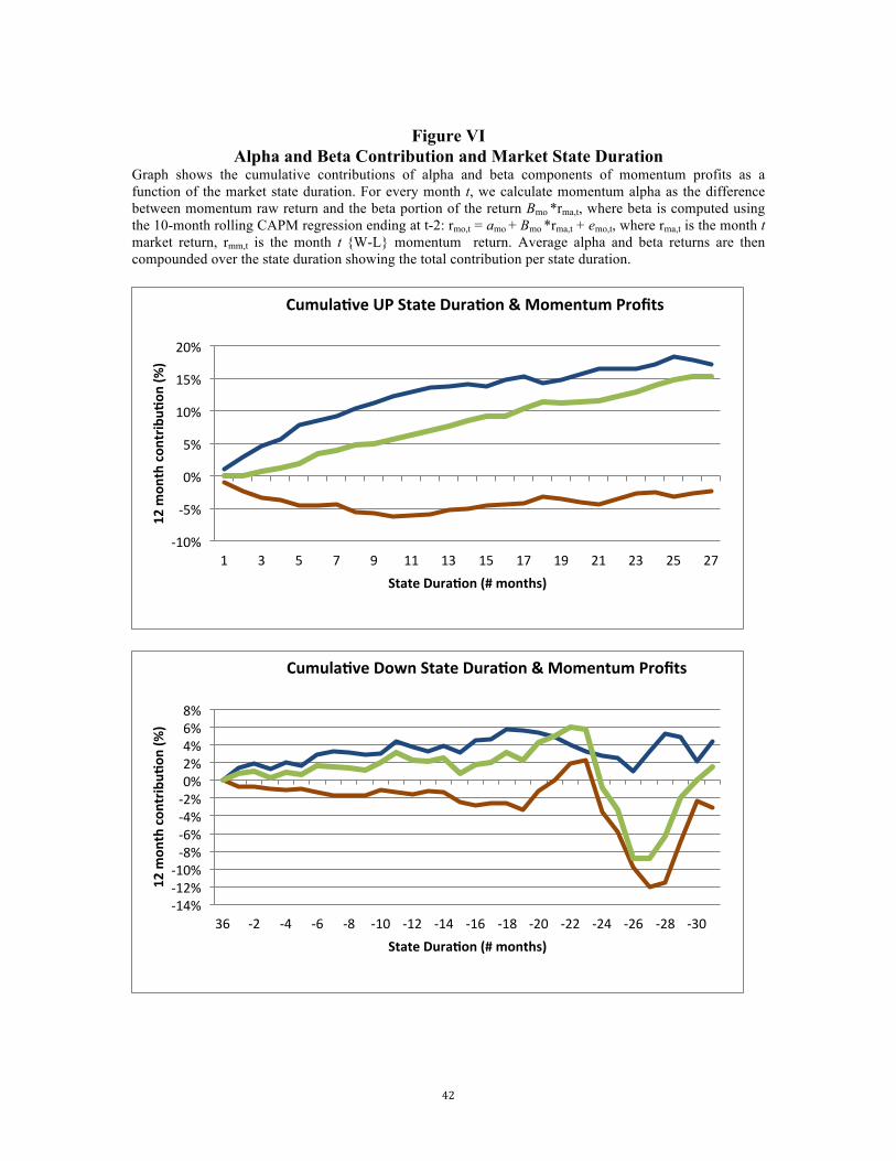
Figure VI

Alpha and Beta Contribution and Market State Duration Graph shows the cumulative contributions of alpha and beta components of momentum profits as a function of the market state duration. For every month t, we calculate momentum alpha as the difference between momentum raw return and the beta portion of the return Bmo *rma,t, where beta is computed using the 10-month rolling CAPM regression ending at t-2: rmo,t = amo + Bmo *rma,t + emo,t, where rma,t is the month t market return, rmm,t is the month t {W-L} momentum return. Average alpha and beta returns are then compounded over the state duration showing the total contribution per state duration.

-­‐10%  

-­‐5%  

0%  

5%  

10%  

15%  

20%  

1   3   5   7   9   11   13   15   17   19   21   23   25   27  

12  m

onth  con

tribu*

on  (%

)  

State  Dura*on  (#  months)  

Cumula*ve  UP  State  Dura*on  &  Momentum  Profits  

-­‐14%  -­‐12%  -­‐10%  -­‐8%  -­‐6%  -­‐4%  -­‐2%  0%  2%  4%  6%  8%  

36   -­‐2   -­‐4   -­‐6   -­‐8   -­‐10   -­‐12   -­‐14   -­‐16   -­‐18   -­‐20   -­‐22   -­‐24   -­‐26   -­‐28   -­‐30  

12  m

onth  con

tribu*

on  (%

)  

State  Dura*on  (#  months)  

Cumula*ve  Down  State  Dura*on  &  Momentum  Profits  

   

    43  

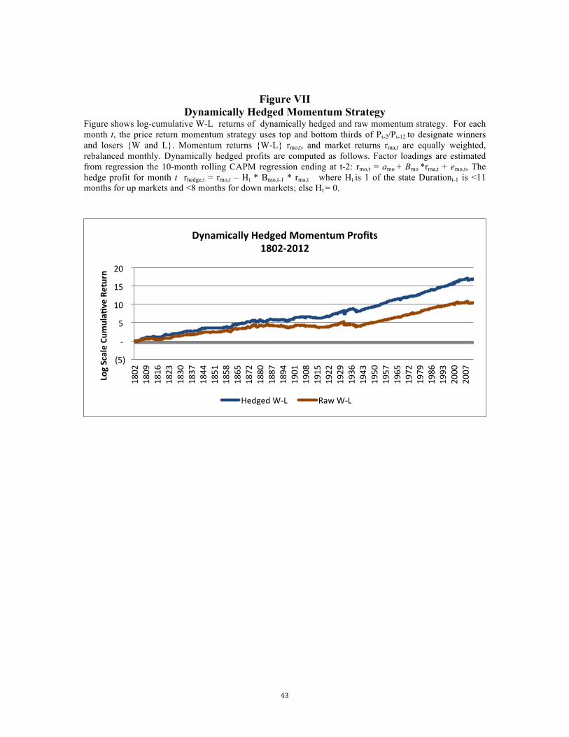
Figure VII Dynamically Hedged Momentum Strategy

Figure shows log-cumulative W-L returns of dynamically hedged and raw momentum strategy. For each month t, the price return momentum strategy uses top and bottom thirds of Pt-2/Pt-12 to designate winners and losers {W and L}. Momentum returns {W-L} rmo,t, and market returns rma,t are equally weighted, rebalanced monthly. Dynamically hedged profits are computed as follows. Factor loadings are estimated from regression the 10-month rolling CAPM regression ending at t-2: rmo,t = amo + Bmo *rma,t + emo,t, The hedge profit for month t rhedge,t = rmo,t – Ht * Bmo,t-1 * rma,t where Ht is 1 of the state Durationt-1 is <11 months for up markets and <8 months for down markets; else Ht = 0.

 (5)  

 -­‐    

 5    

 10    

 15    

 20    

1802  

1809  

1816  

1823  

1830  

1837  

1844  

1851  

1858  

1865  

1872  

1880  

1887  

1894  

1901  

1908  

1915  

1922  

1929  

1936  

1943  

1950  

1957  

1965  

1972  

1979  

1986  

1993  

2000  

2007  

Log  Scale  Cu

mula*

ve  Return  

Dynamically  Hedged  Momentum  Profits    1802-­‐2012  

Hedged  W-­‐L   Raw  W-­‐L