Embed Size (px)
Citation preview

Assessment of the risk of shore contamination
by offshore oil spills: model formulation
A.N Findikakis*, A.W.K. Lav/ & Y. Papadimitrakis^
^Bechtel National Inc., San Francisco
Email: anfindik@bechtei com
N̂anyang Technological University, Singapore
Email: [email protected]. sg
^National Technical University of Athens, Greece
Email: ypapadim@central. ntua.gr
Abstract
A stochastic simulation model has been developed to support theassessment of the risk of shore contamination by offshore oil spills. Themodel simulates the trajectory and evolution of offshore oil spills,accounting for advection by surface currents, spreading, hydrodynamicdispersion, and evaporation. The model uses wind transition matrices toaccount for the uncertainty in the wind direction and speed that mayaffect the movement of an oil slick and its point of contact with theshoreline. After the first contact with the shoreline, the model simulatesthe deformation of the oil slick as it approaches the shore, estimates themass of oil that comes within the wave breaking zone, and, based on thecharacteristics of the shore, the oil deposited on it, and accounts for oiltransport along the coast due to longshore currents. The latter may resultin a much larger portion of the shore impacted than that affected by theinitial contact of the oil spill with the shoreline. Risk estimates are madeby performing Monte Carlo simulations.
Transactions on Ecology and the Environment vol 20, © 1998 WIT Press, www.witpress.com, ISSN 1743-3541

210 Oil & Hydrocarbon Spills, Modelling, Analysis & Control
1 Introduction
Computer simulation models have long been used to estimate theprobability of shoreline contact by accidental oil spills from offshoreplatforms, pipelines, or tankers along frequently traveled routes. Thesimplest oil slick models simulate the trajectory of the centroid of the slick,ignoring size changes due to spreading, and losses due to evaporation,sinking, etc. In these models, the velocity of the centroid is estimated byadding geostrophic, tidal and wind driven currents. The emphasis in manyof these models is on the estimation of the wind driven currents, which inmost cases are the dominant factor that determines the oil slick trajectory.An example of such a model is the model developed by the United StatesGeological Survey [1, 2]. Oil spill trajectory models have been used for bothdeterministic and probabilistic predictions. The latter are made by treatingthe wind vector as a stochastic variable and performing a series of MonteCarlo simulations. A typical application of such simulations is in theprediction of the risk of shore pollution associated with offshore oilproduction. An example is the work of [3], who estimated the probabilitythat different parts of the California coastline may be affected by potentialaccidental oil spills associated with a proposed offshore oil developmentprogram. In that work, an oil spill was represented by a single point whosemovement was simulated until it reached the shoreline.
Another type of models are those that estimate the spreading and weatheringof an oil slick. These models are based on solutions of the continuity andmomentum equations for the oil slick. The simplest of these models are inthe form of algebraic expressions representing solutions of simplifiedversions of the complete flow equations. One of the common simplifyingassumptions, in these models, is that the shape of the oil slick is circular.Stolzenbach et al. [4] presented a review of several models in this category.Models that describe the growth of an oil slick accounting for the combinedeffect of inertial, gravitational, viscous and surface tension forces areusually referred to as spreading models. These models are based on theassumption that some of the forces acting on an oil slick are dominant,during some time period, and that all other forces can be neglected. Theforces that dominate the spreading of an oil slick differ during differentstages of its development. Another type of models are those that calculatethe spreading of oil slicks in the sea due to hydrodynamic dispersion, andthe dispersion of surface oil due to the breakup of the initially coherent oilslick into small droplets and the spread and diffusion of the droplets in thewater column. A summary of the dispersion models can be found in [4, 5].An example of a model combining simple relationships for spreading andhydrodynamic dispersion with expressions for evaporation losses, and
Transactions on Ecology and the Environment vol 20, © 1998 WIT Press, www.witpress.com, ISSN 1743-3541

Oil & Hydrocarbon Spills, Modelling, Analysis & Control 211
emulsification is the model presented by [6]. This model accounts fordifferent oil components, and includes a heat budget calculation for
estimating the temperature of the oil which is used in turn to estimate thedensity, viscosity and surface tension of the oil slick, taking into account theoil composition. Spreading and weathering models, which are based on theassumption of a circular oil slick, can be combined with trajectory models.An example of such a model is the MIT model which accounts for drift,hydrodynamic dispersion, evaporation, biodegradation, photo-oxidation andsedimentation [7].
Accounting for the spreading of an oil slick without making the assumptionthat the slick is circular, requires the solution of the mass balance andmomentum equations for the oil. This was performed by Hess and Kerr whoformulated the equations for two-dimensional spreading of oil on a calmwater surface, and solved them with an Eulerian finite difference scheme[8]. A different approach was followed by some investigators who describedthe growth and motion of an oil slick by solving the two-dimensionaladvection-diffusion equation for oil concentration, neglecting mechanicalspreading [e.g. 9]. Another approach to oil slick transport simulation is theuse of particle tracking methods. Gait et al. used 10,000 particles torepresent the Exxon Valdez spill in Alaska [10]. In this type of model eachindividual particle is described in terms of several attributes, including itslocation, time since release, and status flags indicating if it has reached thecoastline or if it has evaporated, etc. Yapa et al. presented a model based onthe advection-diffusion equations for a two-layer system to describe the fateof oil spills in rivers [11]. The model equations are solved with a Lagrangiandiscrete-parcel algorithm, using a random walk method to representdiffusion.
The model presented in this paper uses a stochastic approach to simulatethe trajectory and evolution of an offshore oil spill, accounting for theeffects of advection by surface currents, spreading, hydrodynamicdispersion, and evaporation of individual oil components. The presentmodel is referred to by the acronym OSM-A (Oil Spill Model -Assessment). It estimates the changes in size an thickness of an oil slickduring its offshore movement, and determines at every time step of thesimulation whether the oil slick has contacted the shoreline. For thispurpose OSM-A considers both the shape, size and thickness of the slickand the geometry of the coastline, and accounts for longshore transport ofthe slick within the wave breaking zone, which may result in a largerportion of the shore(line) impacted than that affected by the initialshoreline contact of the oil slick. The treatment of the interaction of theoil slick with the shore(line) is discussed in detail in the second part of
Transactions on Ecology and the Environment vol 20, © 1998 WIT Press, www.witpress.com, ISSN 1743-3541

212 Oil & Hydrocarbon Spills, Modelling, Analysis & Control
this paper [12].
2 The Oil Spill Simulation Model
Physical processes affecting the fate of oil spills include hydrodynamictransport (advection, spreading, dispersion), evaporation, dissolution,emulsification, auto- and photo-oxidation, biodegradation, sinking,uptake by sediments and aquatic plants, and ingestion by aquatic life.The model accounts for the first four processes, which are treatedindependently of each other. At each simulation step the model firstcomputes the change in the size of the oil slick, assumed to be circular,due to spreading and dispersion. Then it computes the evaporation lossesand adjusts the thickness to account for the evaporated mass.
2.1 Advection
Advection is accounted for by simulating the movement of the centroid ofthe circular oil slick due to the hydrodynamic circulation, and tidal andwind-induced currents. Advection due to the combined effect of winddrift, hydrodynamic circulation and tidal currents is described by theirvector sum.
The wind velocity is represented as a first-order Markov process, simulatedusing three-hour probability transition matrices. The structure of theprobability transition matrices is similar to those used in the USGS oil spillmodel [1]. Each matrix contains 41 states, five wind speeds for each of eightdifferent wind directions and a calm state. Each element of the transitionmatrix gives the probability that a wind of given speed and direction, threehours later may be succeeded by a wind of a different speed and direction.
The wind-induced surface current velocity, Us , is estimated in terms ofthe wind speed [/„ at 10 m above the water surface as:
U,=C.U. (1)
where the empirical constant C,< is estimated from data developed andanalyzed by [13, 14] as:
C,, =0.01exp(1.03 + 0.14UJ (2)
The wind drift vector is rotated by an angle 9 to account for the Coriolis
effect. The deflection angle 9 can be estimated as a function of the windspeed using the empirical expression proposed by [2]:
Transactions on Ecology and the Environment vol 20, © 1998 WIT Press, www.witpress.com, ISSN 1743-3541

Oil & Hydrocarbon Spills, Modelling, Analysis & Control 213
(3)
where g is the acceleration of gravity and v is the kinematic viscosity ofthe water. The deflection angle decreases rapidly for wind speedsbetween 5 to 10 m/s. Wind induced currents become practically parallelto the wind vector for winds greater than 1 5 m/s.
The general circulation and tidal currents contributing to the advectivetransport of an oil slick may be estimated either from data or from ahydrodynamic model. They are treated as input to the oil spill model.
2.2 Spreading
An oil slick tends to spread first due to gravity forces and later due tosurface tension forces at the oil-air and oil-water interface. Immediatelyafter the occurrence of an oil spill the edge of the slick is accelerated underthe influence of gravity. The accelerating phase is followed by a phaseduring which the gravity force is balanced by the dynamic pressure at theedge of the slick due to the motion of the slick relative to the water. Theprincipal force balancing the gravity force during the next phase ofspreading is the viscous shear at the bottom of the slick. Finally, when theslick has become very thin, the spreading is primarily due to surface tensionforces balanced by the viscous shear at the bottom of the slick.
The rate of spreading is estimated using the following assumptions:
a. the oil slick is circular
b. the oil is a homogenous mixture
c. only motions relative to the centroid of the oil slick are considered.
Based on these assumptions the balance of gravity, surface tension,viscous and inertial forces for a circular oil slick leads to the equation:
where R is the radius and h the thickness of the oil slick, / is the time
from the start of oil release, p is the density of the mixture, p^ and v^
are the density and kinematic viscosity of water, /„ is the net surfacetension, per unit length, of the slick boundary computed as the differencebetween the surface tension at the air-oil and water-oil interfaces. Basedon the mean values of the constants proposed by several investigators,
Transactions on Ecology and the Environment vol 20, © 1998 WIT Press, www.witpress.com, ISSN 1743-3541

214 Oil & Hydrocarbon Spills, Modelling, Analysis & Control
Stolzenbach et al. suggested that the constants /?? fa, fa can be takenequal to: 0.42, 1.64 and 0.86, respectively [4].
2.3 Dispersion
The rate of growth due solely to hydrodynamic dispersion is estimated
based on the assumption that the second moment of mass concentration, a;is proportional to a given power of time, /, i.e.
cr = af" (5)
where a and n are constants. Data from dye studies off the California Coastsuggest that n = 2.3 [15]. For a circular oil slick, the rate of growth due tohydrodynamic dispersion can then be expressed as:
f) -^
where k is a dimensional constant.. In the OSM-A model Eq. (6) isapproximated by:
= 6'Z" (7)
where in the open sea the length scale L may be taken equal to the radius
R, k' is a dimensional constant taken equal to 0.01, and n' is anotherconstant equal to 0.33. After contact with the shoreline the scale L isassumed to be proportional to the height of the breaking waves.
2.4 Evaporation
Evaporation losses affect primarily the lighter oil components. Theevaporation of each component is estimated as:
6 =*,(/>/- A- K (8)
where $ is the rate of mass loss due to the evaporation of component /, A/ is
a constant, p\ ,pai are the effective vapor pressure of the oil component / in
a mixture of several components and the vapor pressure of the samecomponent in the air above the slick, and [/„ is the wind speed at 10 m
above the water surface. The constant A, is of the order of 10"̂ (for $ ingm/cm^-s, Ua in cm/s, and p\ and Pa\ in dyne/cm̂ ). The effective vapor
pressure, p\ , of the oil component / is estimated by:
Transactions on Ecology and the Environment vol 20, © 1998 WIT Press, www.witpress.com, ISSN 1743-3541

Oil & Hydrocarbon Spills, Modelling, Analysis & Control 2 1 5
p',=X,p, and X t = - > - (9)
i—wM,
where X^ C, _ M and /?, are the mole fraction, concentration, molecularweight and vapor pressure respectively of component /, and m is the totalnumber of components in the oil mixture. The model keeps track of themass of individual oil components and estimates their concentration bydividing their mass by the volume of the oil slick. The concentrations of theindividual oil components are also used to estimate the density of the oilmixture, as follows:
00)
3 Probability of Shoreline Contact
As the model simulates the movement of the oil slick and its change insize and thickness, it also determines at every time step whether theperiphery of the oil slick has contacted the shoreline. The length of theshoreline affected by an oil spill depends on the size of the oil slick, onthe wind direction after the initial shore contact, as well as on longhshorecurrents that may cause further migration of the oil slick along theshoreline. For example, if the wind continues in a direction normal to theshoreline, then the affected length of the shoreline will be at least equal tothe diameter of the oil slick at the time of initial contact. If, however,after the initial contact the wind reverses direction and blows offshore,then the affected length of the shoreline may be less than the diameter ofthe oil slick. Also, an oil slick that contacts the shoreline, and then movesaway towards the deeper waters due to the reversal of wind direction,may drift in these waters for a while and later contact the shoreline atanother location. To account for these effects the simulation of the oilslick movement and spreading continues beyond the time of the initialcontact with the shoreline. After contact with the shoreline, the modelchanges progressively the shape of the oil slick from a circle to an ellipse,which becomes more and more elongated as the oil slick is pushedagainst the shore. It also estimates the mass of oil that comes within thewave breaking (surf) zone, and accounts for its eventual potentiallongshore transport. This subject is discussed in more detail in the secondpart of this work [12].
Transactions on Ecology and the Environment vol 20, © 1998 WIT Press, www.witpress.com, ISSN 1743-3541
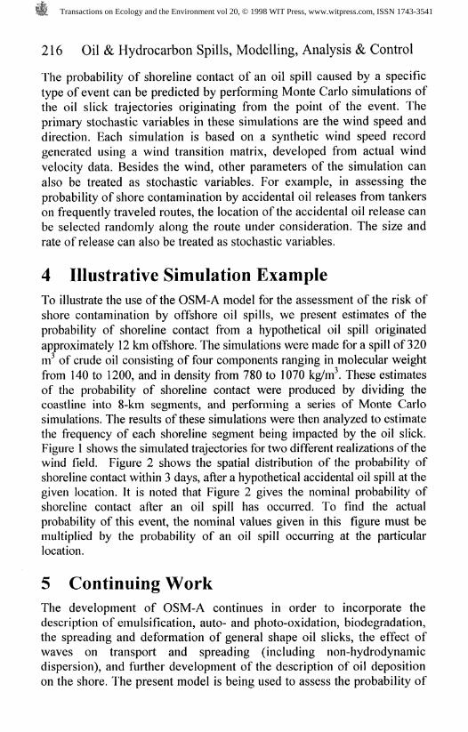
216 Oil & Hydrocarbon Spills, Modelling, Analysis & Control
The probability of shoreline contact of an oil spill caused by a specifictype of event can be predicted by performing Monte Carlo simulations ofthe oil slick trajectories originating from the point of the event. Theprimary stochastic variables in these simulations are the wind speed anddirection. Each simulation is based on a synthetic wind speed recordgenerated using a wind transition matrix, developed from actual windvelocity data. Besides the wind, other parameters of the simulation canalso be treated as stochastic variables. For example, in assessing theprobability of shore contamination by accidental oil releases from tankerson frequently traveled routes, the location of the accidental oil release canbe selected randomly along the route under consideration. The size andrate of release can also be treated as stochastic variables.
4 Illustrative Simulation Example
To illustrate the use of the OSM-A model for the assessment of the risk ofshore contamination by offshore oil spills, we present estimates of theprobability of shoreline contact from a hypothetical oil spill originatedapproximately 12 km offshore. The simulations were made for a spill of 320m^ of crude oil consisting of four components ranging in molecular weightfrom 140 to 1200, and in density from 780 to 1070 kg/nf. These estimatesof the probability of shoreline contact were produced by dividing thecoastline into 8-km segments, and performing a series of Monte Carlosimulations. The results of these simulations were then analyzed to estimatethe frequency of each shoreline segment being impacted by the oil slick.Figure 1 shows the simulated trajectories for two different realizations of thewind field. Figure 2 shows the spatial distribution of the probability ofshoreline contact within 3 days, after a hypothetical accidental oil spill at thegiven location. It is noted that Figure 2 gives the nominal probability ofshoreline contact after an oil spill has occurred. To find the actualprobability of this event, the nominal values given in this figure must bemultiplied by the probability of an oil spill occurring at the particularlocation.
5 Continuing Work
The development of OSM-A continues in order to incorporate thedescription of emulsification, auto- and photo-oxidation, biodegradation,the spreading and deformation of general shape oil slicks, the effect ofwaves on transport and spreading (including non-hydrodynamicdispersion), and further development of the description of oil depositionon the shore. The present model is being used to assess the probability of
Transactions on Ecology and the Environment vol 20, © 1998 WIT Press, www.witpress.com, ISSN 1743-3541

Oil & Hydrocarbon Spills, Modelling, Analysis & Control 217
shoreline contamination by potential accidental oil releases by tankers
and other ships in Greek seas, and more specifically in the Gulf ofSaronikos and in the Gulf of Kavala, where an oil production platformexist. In this application OSM-A is used in conjunction with thePrinceton Ocean Model [16] which is used to simulate surface currentsand undercurrents associated with the general circulation in Saronikosand in the Gulf of Kavala, under a variety of external forcing conditions.
JV
t
m lies0 102030l.4_l-.J_]_J~J
km
Shoreline contactafter 67 hours
Shoreline contactafter 46 hours
Oil SpillLocation
shorelineNote:
A - assumed accidental oil release on March 16, 1982B - assumed accidental oil release on April 10, 1982
Figure 1. Simulated trajectories of an oil slick originating at an offshorelocation using wind data from two actual historic storms.
Transactions on Ecology and the Environment vol 20, © 1998 WIT Press, www.witpress.com, ISSN 1743-3541

218 Oil & Hydrocarbon Spills, Modelling, Analysis & Control
t
0 10 20I ________ I ..I _________ !._.... I
m iles0 1 0 2 0 3 0L._l.._l ..... L__L_J_J
km
Notes:
1 . The number on each circle represents the probability that a spill, 72hours after its release, will be offshore within the corresponding circle.
2. The first number at the top of each bar represents the probability (%)that an oil spill may contact the corresponding 8-km shorelinesegment.
3. The number in parenthesis represents the minimum contact
Figure 2. Probability map of oil slick location, and distribution ofprobability of shoreline contact (based on 200 simulated trajectories).
Acknowledgments
The authors would like to acknowledge the contributions of Mr. CheeSiang Toh at Nanyang Technical University in Singapore, and Miss E.Kehagia, Dr. G. Kantzios and Mr. A. Papadopolis-Detzorgis at theNational Technical University of Athens, Greece, who work on differentaspects of this program.
Also, the first and the last author would like to acknowledge theSecretariat of Research and Technology of Greece for its support. Thefunding support to the second author through the Academic ResearchFund from the Nanyang Technological University is also appreciated.
References
[1] Smith, R.A., Slack, J.R., Wyant, T. and Lanfear, K.J., The Oil SpillRisk Analysis Model of the U.S. Geological Survey, U.S.
^ 107, 1982.
Transactions on Ecology and the Environment vol 20, © 1998 WIT Press, www.witpress.com, ISSN 1743-3541

Oil & Hydrocarbon Spills, Modelling, Analysis & Control 219
[2] Samuels, W.B., Huang N.E. and Amstutz, D.E., An Oil SpillTrajectory Analysis Model with Variable Wind Deflection Angle,Ocean Engineering, Vol. 9, No. 4, pp. 347-360, 1982.
[3] LaBelle, R.P., Lanfear, K.J., Banks A.D. and Karpas, R.M., An OilSpill Risk Analysis for the Southern California Lease Offering,Minerals Management Service, Environmental Modeling Group,U.S. Geological Survey, Open File Report # 83-563, 1983.
[4] Stolzenbach, K.D., Madsen, O.S, Adams, E.E., Pollack, A.M. andCooper, C.K., A Review and Evaluation of Basic Techniques forPredicting the Behavior of Surface Oil Slicks, MIT Sea GrantProgram, Report No. MITSG 77-8, Massachusetts Institute ofTechnology, Cambridge, Massachusetts, 1977.
[5] ASCE Task Committee on Modeling of Oil Spills of the WaterResources Engineering Division, State-of-the-Art Review ofModeling Transport and Fate of Oil Spills, Journal of HydraulicEngineering, Vol. 122, No. 11, pp. 594-609, November 1996.
[6] Rasmussen, D., Oil Spill Modeling-A tool for Cleanup Operations,Proceedings of the 1985 Oil Spill Conference, American PetroleumInstitute, Washington, D.C., pp. 243-249, 1985.
[7] Psaraftis, H.N., Nyhart, J.D. and Betts, D.A., First Experiences withMassachusetts Institute of Technology Oil Spill Model,Proceedings of the 1983 Oil Spill Conference, American PetroleumInstitute, pp. 301-305, 1983.
[8] Hess, K.W. and Kerr, C.L., A Model to Forecast the Motion of Oilin the Sea, Proceedings of the 1979 Oil Spill Conference, AmericanPetroleum Institute, Washington, D.C., pp. 653-663, 1979.
[9] Kollmeyer, R.C. and Thompson, M.E., New York Harbor Oil DriftPrediction Model, Proceedings of the 1977 Oil Spill Conference,American Petroleum Institute, Washington, D.C., pp. 441-445,1977.
[10] Gait, J.A., Watabayashi, G.Y., Payton D.L. and Peterson, J.C.,Trajectory Analysis for the Exxon Valdez: Hindcast Study,Proceedings of the 1991 Oil Spill Conference, American PetroleumInstitute, Washington, D.C., pp. 629-634, 1991.
[ll]Yapa, P.D., Shen, H.T., Daly, S.F. and Hung, S.C., Oil SpillSimulation in Rivers, Proceedings of the 1991 Oil Spill Conference,American Petroleum Institute, pp. 593-600, 1991.
Transactions on Ecology and the Environment vol 20, © 1998 WIT Press, www.witpress.com, ISSN 1743-3541

220 Oil & Hydrocarbon Spills, Modelling, Analysis & Control
[12] Law, A.W.K, A. N. Findikakis and Papadimitrakis, Y., Assessmentof the Risk of Shore Contamination by Offshore Oil Spills.Simulation of Nearshore Transport. To be presented.
[13] Wu, J., Wind Induced Drift Currents, J. Fluid Mechanics, 68, pp. 49-70, 1975.
[14] Wu, J., Wind-Stress Coefficients over Sea-Surface near NeutralConditions - A Revisit, J. Phys. Oceanography, 10, pp. 727-740,1980.
[15] Okubo, A., A Review of Theoretical Models of Turbulent Diffusionin the Sea, Chesapeake Bay Institute, John Hopkins University,Technical Report No. 30, 1962.
[16] Blumberg, A.F. and Mellor, G.L., A Description of a Three-Dimensional Coastal Ocean Circulation Model, Three-Dimensional
MxM?, ed. N. Heaps, AGU, pp. 208, 1987.
Transactions on Ecology and the Environment vol 20, © 1998 WIT Press, www.witpress.com, ISSN 1743-3541