Florida State University Libraries

2016

Characterizing the Onset and Demise of theIndian Summer MonsoonRyne Garrett Noska

Follow this and additional works at the FSU Digital Library. For more information, please contact lib-ir@fsu.edu

FLORIDA STATE UNIVERSITY

COLLEGE OF ARTS AND SCIENCES

CHARACTERIZING THE ONSET AND DEMISE

OF THE INDIAN SUMMER MONSOON

By

RYNE G. NOSKA

A Thesis submitted to the Department of Earth, Ocean and Atmospheric Sciences

in partial fulfillment of the requirements for the degree of

Master of Science

2016

ii

Ryne G. Noska defended this thesis on March 24, 2016.

The members of the supervisory committee were:

Vasubandhu Misra

Professor Directing Thesis

Robert Hart

Committee Member

Mark Bourassa

Committee Member

The Graduate school has verified and approved the above-named committee members, and

certifies that the thesis has been approved in accordance with university requirements.

iii

I dedicate this work to

Jesus

The Rock of Ages

Upon whom I stood

In the midst of the deluge

During these formative years of my life:

You never fail me!

“From the end of the earth

I call to You when my heart is faint;

Lead me to the rock that is higher than I.”

~Psalm 61:2

iv

ACKNOWLEDGMENTS

I am grateful first and foremost for my Lord Jesus Christ, who has been a firm

foundation throughout my stay at Florida State University. I would find no purpose in my

research or in anything else without Him, for in Him I live and move and have my being. My

family, and especially my wife Jenna, were invaluable during my graduate years. They

reminded me of the world outside of meteorology and that I should, indeed must, be engaged

in it. What a joy it is to be reminded of what matters most in life through their affection and

support!

I thank Dr. Vasubandhu Misra for his willingness to guide me as I encountered

complex challenges and to offer suggestions that further improved my research. I do not doubt

that I completed so much research in such a short period of time because of your motivating

encouragement. Drs. Bob Hart and Mark Bourassa have also offered many suggestions and

corrections that made the outcome of my research much greater than it began; thank you. I

further acknowledge the immense assistance Drs. Amit Bhardwaj and Akhilesh Mishra

offered through many useful discussions and programming support; I consider you both as

friends.

I gratefully acknowledge the financial support given by NOAA (NA12OAR43310078)

and the Earth System Science Organization, Ministry of Earth Sciences, Government of India

(Grant number MM/SERP/FSU/2014/SSC-02/002) to conduct this research under Monsoon

Mission. Finally, I thank the Indian Meteorological Department for the availability of the

daily rain analysis over India.

v

TABLE OF CONTENTS

List of Tables ............................................................................................................................ vi List of Figures ......................................................................................................................... vii Abstract ..................................................................................................................................... x 1. INTRODUCTION ................................................................................................................ 1 2. DATA ................................................................................................................................... 5 3. METHODOLOGY ................................................................................................................ 9

3.1. Defining the All-India Rainfall Onset and Demise Index............................................ 9 3.2. Insensitivity to False Onsets ...................................................................................... 11 3.3. Seasonal Evolution ..................................................................................................... 13 3.4. Interannual Variability .............................................................................................. 16

4. RESULTS AND DISCUSSION ......................................................................................... 19

4.1. Insensitivity to Arbitrary Domain Changes, Time Period Changes, and False Onsets ......................................................................................................................... 19

4.2. Seasonal Evolution ..................................................................................................... 20 4.2.1 The Land-Ocean Temperature Contrast ........................................................ 23 4.2.2 Large-Scale Atmospheric Circulation Reversal .............................................. 24 4.2.3 Large-Scale Oceanic Circulation Reversal ..................................................... 25 4.2.4 Moisture Convergence and Subsequent Precipitation ................................... 28

4.3. Interannual Variability .............................................................................................. 30 4.3.1 Features of the Indian Summer Monsoon ...................................................... 30 4.3.2 Temperature .................................................................................................... 32 4.3.3 Wind ................................................................................................................ 33 4.3.4 Oceanic Phenomena ........................................................................................ 34 4.3.5 Moisture........................................................................................................... 35

5. CONCLUSION .................................................................................................................. 38 APPENDICES ......................................................................................................................... 41 A. Tables ................................................................................................................................. 41 B. Figures ............................................................................................................................... 49 References ................................................................................................................................ 90 Biographical Sketch................................................................................................................. 96

vi

LIST OF TABLES

1 Large-scale atmospheric and oceanic changes associated with onset from previous literature. .......................................................................................................................... 41

2 Onset indices from previous literature. ........................................................................... 43

3 Datasets implemented in this paper and their metadata. ............................................ 45

4 False onset years and their three pertinent dates: false onset, “actual” onset, and AIRO. ................................................................................................................................ 45

5 Direct and derived large-scale atmospheric and oceanic variables analyzed in this

study. ................................................................................................................................. 46

6 Correlations between ISM features. Bolded values are significant at the 95% confidence interval. ............................................................................................................................. 46

7 Annual total seasonal AIR, AIRO, AIRD, and season length. ......................................... 47

vii

LIST OF FIGURES 1 Important locations referred to during this study. .......................................................... 49 2 The domains and rain gauge distributions used in APHRODITE V1101 for monsoon

Asia (MA), the MIddle East (ME), and northern Eurasia [i.e., Russia (RU)], and in V1005 for Japan (JP). ........................................................................................................ 49

3 Seasonal cycle of rainfall for the year 2000. ................................................................. 50 4 The seasonal cycle of rainfall during the Maharashtra Drought of 1972. ...................... 50 5 OLR in the middle of May for the four cases of multiple monsoon onset. ....................... 51 6 AIR-based a) onset date, b) demise date, and c) season length from 1902 to 2005. ........ 52 7 Distribution of onset dates (top), demise dates (middle), and season length (bottom). .. 53

8 Parameters characterizing a Gaussian or normal distribution. ....................................... 54 9 Brown shaded area represents the AIR region. ................................................................ 55

10 Comparison of onset (top) and demise (bottom) dates for two spatially-averaged rainfall

domains: AIR and APHRO. .............................................................................................. 56 11 Seasonal evolution of 11 false onset years recorded by previous studies. ....................... 57

12 Ekman transport throughout the mixed layer (roughly 100m) of the ocean, where the

competing Coriolis force and turbulent drag slow and turn the direction of the current to the right at deeper depths. ............................................................................................... 58

13 Simplified regulation of the seasonal cycle of the Indian Ocean in the boreal a) summer

and b) winter, where black arrows indicate the direction of near-surface winds and gray arrows indicated the direction of Ekman transport and the resulting heat flux. ........... 58

14 Seasonal evolution of the daily composite (averaged over 104 years from 1902-2005) of

300hPa temperature centered on the AIRO (time = 0) at intervals of five days. ............ 59

15 Same as Fig. 14, but centered on the AIRD. .................................................................... 60

16 The climatological daily zonal progression of the meridional temperature gradient between 5°N and 25°N at 300hPa as a function of lead/lag time with respect to the a) AIRO and b) AIRD from 40°E to 120°E. ........................................................................... 61

17 Same as Fig. 14, but for 850hPa to 200hPa vertical wind shear. .................................... 62

18 Same as Fig. 14, but for 850hPa to 200hPa vertical wind shear centered on the AIRD. ................................................................................................................................ 63

viii

19 Same as Fig. 14, but for kinetic energy of 850hPa winds. ............................................... 64 20 Same as Fig. 14, but for kinetic energy of 850hPa winds centered on the AIRD. ........... 65

21 The climatological daily meridional progression of zonally-averaged meridional ocean

heat transport computed to a depth of 105m (~mixed layer depth of the tropical Indian Ocean) as a function of lead/lag time with respect to the a) AIRO and b) AIRD from 25°S to 25°N. ............................................................................................................................. 66

22 Schematic of the horizontal velocity structure of the n=1 Rossby mode with southward

Ekman flow added to regions outside of the equatorial wave guide and cool colored pathways and streamlines indicating southward heat transport. .................................. 66

23 Same as Fig. 14, but for vertically integrated moisture flux convergence. ..................... 67

24 Same as Fig. 14, but for vertically integrated moisture flux convergence centered on the

AIRD. ................................................................................................................................ 68

25 Same as Fig. 14, but for precipitable water. .................................................................... 69

26 Same as Fig. 14, but for precipitable water centered on the AIRD. ................................ 70

27 Same as Fig. 14, but for rainfall. ...................................................................................... 71

28 Same as Fig. 14, but for rainfall centered on the AIRD. ................................................. 72

29 Correlation of a) AIRO and b) AIRD date anomalies with total seasonal rainfall anomalies. ......................................................................................................................... 73

30 Same as Fig. 29, but with 300hPa meridional temperature gradient from 5°N to 25°N at

various lead/lag times with respect to the a) AIRO and b) AIRD date. .......................... 73

31 Correlation of AIRO date anomalies with 300hPa temperature anomalies at various lead/lag times. ................................................................................................................... 74

32 Same as Fig. 31, but with AIRD date anomalies. ............................................................ 75

33 Same as Fig. 31, but with 850hPa to 200hPa vertical wind shear anomalies. ............... 76

34 Same as Fig. 31, but with 850hPa to 200hPa vertical wind shear anomalies and AIRD

date anomalies. ................................................................................................................. 77

35 Same as Fig. 31, but with kinetic energy anomalies of 850hPa wind. ............................ 78

36 Same as Fig. 31, but with kinetic energy anomalies of 850hPa wind and AIRD date anomalies. ......................................................................................................................... 79

37 Same as Fig. 29, but with meridional ocean heat transport from 25°S to 25°N at various

lead/lag times with respect to the a) AIRO and b) AIRD date. ........................................ 80

ix

38 Correlation of AIRO date anomalies with global December-February averaged sea surface temperature anomalies. ....................................................................................... 80

39 Correlation of monthly Niño3.4 sea surface temperature (SST) anomalies with AIRO

date anomalies (red circles), AIRD date anomalies (black squares), total seasonal AIR anomalies (blue circles), and June-September (JJAS) AIR anomalies (green

diamonds). ......................................................................................................................... 81

40 A comparison of the total seasonal AIR (blue) and the June-September (JJAS) All-India Monsoon Rainfall (AIMR; orange). ................................................................................... 82

41 Same as Fig. 31, but with vertically integrated moisture flux convergence anomalies. ......................................................................................................................... 83

42 Same as Fig. 31, but with vertically integrated moisture flux convergence anomalies

and AIRD anomalies. ........................................................................................................ 84

43 Same as Fig. 31, but with precipitable water anomalies. ................................................ 85

44 Same as Fig. 31, but with precipitable water anomalies and AIRD anomalies. ............. 86

45 Same as Fig. 29, but with AIR anomalies at various lead/lag times with respect to the a) AIRO and b) AIRD date. ................................................................................................... 87

46 Same as Fig. 31, but with rainfall anomalies. ................................................................. 88

47 Same as Fig. 31, but with rainfall anomalies and AIRD date anomalies. ...................... 89

x

ABSTRACT

An objective index of the onset and demise of the Indian summer monsoon (ISM) is

introduced. This index has the advantage of simplicity by using only one readily available

variable, All-India rainfall (AIR), which has been reliably observed for more than a century.

The proposed All-India rainfall onset and demise (AIROD) is shown to be insensitive to all

recorded false onsets. By definition, the seasonal ISM rainfall anomalies become a function

of the variations of onset and demise dates, with early onset and late demise resulting in

greater season length and total seasonal rainfall. Seasonal rainfall itself is a strong predictor

of the following ENSO phase and provides a more accurate depiction of the ISM than does

the commonly-used June-September (JJAS) All-India monsoon rainfall (AIMR) index.

This new index provides an accurate and comprehensive representation of the

seasonal evolution of the ISM by capturing dramatic changes in large-scale dynamic (i.e.

wind- and current-based) and thermodynamic (temperature- and moisture-based) variables,

which is found to make the onset an especially important feature to monitor to understand

the evolution of the ensuing monsoon season. In particular, the zonal (meridional)

progression of 300hPa meridional temperature gradient (meridional ocean heat transport)

reversal may be monitored about twenty days before onset to help determine the timing of

its arrival.

Interannual variability of ISM features and their associated large-scale phenomena

are also analyzed. An early (late) onset corresponds to an increase (decrease) in anomalies of

kinetic energy of 850hPa wind over the Arabian Sea and central Indian rainfall up to fifteen

and ten days before onset, respectively. Conversely, an early (late) demise corresponds to a

decrease (increase) in the aforementioned anomalies up to ten days after demise.

xi

Additionally, the preceding December-February ENSO phase is associated with the onset of

the ISM, as an early (late) onset is preceded by La Niña (El Niño).

1

CHAPTER 1

INTRODUCTION The Indian summer monsoon (ISM), which is derived from the Arabic word translated

“season”, is defined as the reversal of the large-scale wind pattern to southwesterlies off the

Somali Coast. A sudden increase in rainfall occurs as a visible manifestation of this shift in

wind direction and impacts many aspects of Indian society. The ISM, which climatologically

occurs from June to September, affects over 1.25 billion people in India, providing 70-90% of

the nation’s annual mean rainfall (Kumar et al., 2013). Agriculture, which accounts for over

20% of India’s gross domestic product and employs over half of its workforce, is particularly

impacted as over 60% of agricultural production is rain-fed by the monsoon (Kumar et al.,

2004). Therefore a comprehensive understanding and consequent accurate prediction of

monsoon characteristics are essential.

The onset and demise of the ISM in particular are of such importance that the Indian

Meteorological Department (IMD) has determined them for more than 100 years

(Ananthakrishnan and Soman, 1988; Pai and Rajeevan, 2009). These transitions are

associated with significant changes in large-scale atmospheric and oceanic phenomena, and

their potentially unanticipated variability oftentimes leads to economic, agricultural,

governmental, and societal stress (Gadgil and Kumar, 2006). Some of the most drastic

changes occur with temperature, wind, moisture, and oceanic variables (Table 1). Many onset

and demise indices have been suggested in an attempt to accurately portray these essential

features of the ISM (Table 2). While onset and demise dates are not unique in that they may

be determined using a number of indices and variables, any suggested index should capture

the aforementioned drastic, large-scale atmospheric and oceanic changes.

2

There are a number of limitations for previously suggested onset and demise indices.

Without objective thresholds, an index cannot provide an exact date of onset and is subject

to forecaster bias (Rao, 1976). Second, many indices consider a single variable without

providing an atmospheric and oceanic context, which may result in a narrow scope of

application (Ananthakrishnan et al., 1968; Ramage, 1971; Ananthakrishnan and Soman,

1988; Fasullo and Webster, 2003; Janowiak and Xie, 2003; Zeng and Lu, 2004; Taniguchi and

Koike, 2006; Xavier et al., 2007; Wang et al., 2009; Goswami and Gouda, 2010; Moron and

Robertson, 2014; Misra and DiNapoli, 2014). Fasullo and Webster (2003) argues that onset

and demise dates based on rainfall alone are susceptible to both poor measurements and

modeling, which vertically integrated moisture transport ameliorates. On the other hand, the

hydrological index as suggested in Fasullo and Webster (2003), among many others,

encounters difficulty in capturing the synoptic variability and spatial complexity of monsoon

transitions (Ramage, 1971; Zeng and Lu, 2004; Prasad and Hayashi, 2005; Taniguchi and

Koike, 2006; Xavier et al., 2007; Wang et al., 2009).

Another critical limitation is susceptibility to false onsets (Ananthakrishnan et al.,

1968; Ramage, 1971; Rao, 1976; Ananthakrishnan and Soman, 1988; Wang et al, 2009;

Goswami and Gouda, 2010; Misra and DiNapoli, 2014). A false onset is a brief increase in

rainfall that precedes onset and is followed by a lengthened period of dryness (Joseph et al.,

1994; Flatau et al., 2001, 2003; Moron and Robertson, 2014). False onsets are also referred

to in scientific studies as double onsets, bogus onsets, and pre-monsoon rain peaks (PMRP)

(Joseph and Pillai, 1988; Flatau et al., 2001; Fasullo and Webster, 2003; Pai and Rajeevan,

2009). Such occurrences are a result of synoptic disturbances on small time scales; thus, any

index which does not cover a large enough region and time period is likely susceptible.

Similarly, many indices account only for Kerala, a small region on the southwestern tip of

the Indian subcontinent, and therefore are not necessarily indicative of onset for the region

3

as a whole (Ananthakrishnan et al., 1968; Rao, 1976; Ananthakrishnan and Soman, 1988;

Joseph et al., 2006; Pai and Rajeevan, 2009; Goswami and Gouda, 2010).

As Fasullo and Webster (2003) mention, some indices are also based upon poor

measurements or time steps much longer than the daily time step for which onset and

withdrawal occur (Rao, 1976; Janowiak and Xie, 2003; Zeng and Lu, 2004). While these

limitations are sufficient for coarse global studies, practical applications require better

resolution and data density. Contemporary datasets and models allow this limitation to be

overcome (Rajeevan et al., 2008; Saha et al., 2010; Yatagain et al., 2012). Finally, many

indices are not intended for forecasting purposes but rather for modeling and research

applications, usually as a result of a variable’s required persistence (Ramage, 1971;

Ananthakrishnana and Soman, 1988; Janowiak and Xie, 2003; Zeng and Lu, 2004; Taniguchi

and Koike, 2006; Wang et al., 2009; Goswami and Gouda, 2010; Moron and Robertson, 2014;

Misra and DiNapoli, 2014). While the index explored in this study provides no objective

solution to this limitation, it shall be shown that subjective monitoring may be possible.

A new index for onset and demise based on IMD daily rainfall over the entire Indian

subcontinent is introduced for the following reasons: 1) rainfall exerts a practical influence

on all sectors of Indian society; 2) those outside the scientific community have greater

comprehension and experience of a precipitation-based index; 3) rainfall is one of few directly

and reliably observed daily variables available since the early twentieth century over India,

4) the selected region is large enough and the rainfall threshold robust enough to avoid

synoptic-triggered false onsets; and 5) the IMD gridded rainfall dataset implemented has

excellent spatiotemporal resolution. A daily precipitation-based onset date is also easily

comparable to the IMD onset definition. However, the larger domain for all-India rainfall

(AIR) should result in later onset dates than IMD rainfall, which only considers preliminary

rainfall in Kerala, and should thus be more representative of India’s collective onset and

4

demise dates and more resistant to false onsets. All large-scale atmospheric and oceanic

changes are then characterized in this new index’s context to provide a comprehensive view

of monsoon transitions, a view which is lacking in most other previous studies. In this way,

numerous variables instead of rainfall alone are used to portray its far-reaching implications

and its accurate representation of large-scale atmospheric and oceanic changes.

Furthermore, the index suggested is flexible in that it may be applied to any strongly seasonal

variable of interest. Fasullo and Webster (2003) provides the following criteria that every

successful onset and demise index must meet:

association with transition of large-scale monsoon circulation processes;

insensitivity to fluctuations within the monsoon season and to false onsets caused by

individual synoptic disturbances; and

foundation upon well-observed, long-duration fields that experience sudden, extreme

variability during monsoon transitions.

The onset and demise index presented in this study meets each condition in a clear and

applicable fashion.

This study objectively determines the onset and demise of the Indian summer

monsoon in a manner that avoids false onsets, allows holistic characterization of and real-

time monitoring of seasonal evolution, and accurately captures interannual variability.

Chapter 2 reviews the datasets used in this research. The methodology implemented to

determine and characterize onset and demise dates is elucidated in chapter 3. Results

concerning the index’s insensitivity to false onsets, the seasonal evolution of the ISM, and

the variability of features of the ISM are discussed in chapter 4. Conclusions are included in

the final chapter.

5

CHAPTER 2

DATA

Different datasets are used for atmospheric and oceanic variables (Table 3). Gridded

AIR is obtained from the Indian Meteorological Department (IMD) National Climate Centre

(NCC) 0.25° gridded rainfall dataset (Pai et al., 2014a,b), which was directly provided by a

known contact at the NCC for the years 1902 to 2005. The data is interpolated to a 0.25° grid

spacing using over 2,500 quality-controlled stations (Pai et al., 2014a,b). Recall that this

rainfall is one of the only directly observable daily variables during the full 104 years of this

study over India. In order to ensure the resistance of the rainfall-based onset and demise

dates to changes in domain, the Research Institute for Humanity and Nature (RIHN) and

Meteorological Research Institute of Japan Meteorological Agency’s (MRI/JMA) Asian

Precipitation – Highly Resolved Observational Data Integration Towards Evaluation of

Water Resources (APHRODITE) version 1101 station data was compared to IMD AIR. The

station data was interpolated to 0.25 grid spacing from 1951-2005 and included both India

and Bangladesh in its domain (Yatagai et al., 2012). This data was supplied and downloaded

from the Center for Ocean and Atmospheric Prediction Studies (COAPS) at Florida State

University (FSU). Caution should be taken with gridded data as the density of stations are

not homogenous throughout the region of study. Note that there are far fewer stations in

eastern India and southeastern Bangladesh as can be seen in Fig. 2.

All other atmospheric variables were downloaded by batch from the European Centre

for Medium-Range Weather Forecasts’ (ECMWF) Atmospheric Reanalysis of the 20th

Century (ERA-20C; Poli et al., 2013), ECMWF’s first extended climate reanalysis (Dee et al.,

2014), using the python library “ecmwfapi”. Only surface observations are assimilated using

an Ensemble of Data Assimilations (EDA) of 10 members which are forced by a HadISST

6

2.1.0.0 ensemble of sea-surface temperature and sea-ice conditions. Each member employs a

24-hour four-dimensional variational (4D-Var) analysis scheme. Assimilated surface

observations are provided by the International Surface Pressure Databank (ISPD) 3.2.6

(atmospheric surface pressure) and the International Comprehensive Ocean-Atmosphere

Data Set (ICOADS) 2.5.1 (atmospheric surface pressure, atmospheric and ocean

temperatures, and atmospheric near-surface winds all only above oceans). The pressure

observations are bias-corrected using a variational bias correction within the assimilation,

and the wind observations above oceans are assimilated as they are verified to improve the

quality of the atmospheric circulation representation, particularly in the tropics (Poli et al.,

2013). This dataset is interpolated from approximately 125km resolution (using a spectral

triangular truncation T159) and 3-hour time step to a 0.25 grid spacing and daily time step

from 1902 to 2005 to match the observational rainfall’s spatiotemporal gridding. The domain

for precipitable water, vertically integrated moisture flux divergence, and the zonal and

meridional components of wind velocity is 50-110E and 0-40N. 300hPa temperature’s

longitudinal extent is broadened from 40-120E so that all pertinent information noted by

Yanai et al. (1992) is accounted for.

A few cautionary statements must be made concerning this relatively new

atmospheric reanalysis. First, data in the upper tropospheric/lower stratospheric 100-200hPa

levels are to be viewed with caution as they are highly model-dependent (Poli et al., 2013).

All validation conducted in this study, with the exception of 850-200hPa vertical wind shear,

are in the lower troposphere (well below these cautionary levels). Second, long-term climate

trends are not completely captured by the reanalysis, which produces increments away from

the surface due to insufficient attention during system development to diagnose the quality

of low-frequency climate information in advance (Poli et al., 2015). Poli et al. (2013) does

7

indicate, however, that representation of daily meteorological events, including extremes, is

of reasonable quality. ERA-20C seems to be an excellent reanalysis for this study because

the primary focus of this research is on a daily time scale and large variations in variables

rather than with exact quantities are desired. Quantitative errors are not as crucial as errors

in pattern representation, and as previously stated the reanalysis accurately portrays daily

events. It is also the only reanalysis available at T159 (125km) resolution for over a century

and is conducted with a relatively modern version of the ECMWF model which incorporates

4D-variational analysis. Finally, ERA-20C is a pilot reanalysis, and is not intended to

produce a final ‘best-product’ state-of-the-art climate dataset. Rather, its primary purpose is

the study of the feasibility of reanalyzing the century using new data assimilation methods

to tackle the problem of observing system changes (Poli et al., 2013). As indicated above,

however, the atmospheric reanalysis performs very well on the daily timescale and is thus

effective for this research.

Meridional ocean current and potential temperature are extracted from the National

Centers for Environmental Prediction’s (NCEP) Climate Forecast System Reanalysis (CFSR;

Saha et al., 2010), the first global reanalysis based on a coupled model of the atmosphere-

ocean-land surface-sea ice system. This data, as with APHRODITE, is available from COAPS

at FSU. Its assimilation scheme is considered weakly coupled in that it uses the coupled

model only for generating background estimates for each analysis cycle while the analysis

itself is uncoupled. As a result, information from observations in any one component can only

affect other components indirectly by propagating information to the next analysis cycle (Dee

et al., 2014). The resolution is 0.25 at the equator, but resolution decreases to 0.5 beyond

the tropics (Saha et al., 2010). Therefore, all data ingested in this study was interpolated to

a uniform 0.5 grid spacing for consistency. Potential temperature and meridional current

8

velocity were calculated for a domain of 40-100E and 25S-25N. Eleven of the available

forty depth levels were used, down to a depth of 105m., and the variables were computed

daily from 1979 to 2005. The Met Office Hadley Centre’s sea ice and sea surface temperature

(SST) data set version 1 (HadISST1; Rayner et al., 2003; Reynolds et al., 2007) is available

from COAPS at FSU and provides 1 square grids of monthly-averaged, global SSTs from

1871 to the present, but only years since 1902 are used in this study for comparison with the

primary dataset, IMD AIR. Finally, the National Center for Atmospheric Research (NCAR)

Climate and Global Dynamics (CGD) Climate Analysis Section (CAS) supplies a record of

Niño 3.4 monthly SSTs (N3.4) (Trenberth and Stepaniak, 2000). The domain over which the

Niño 3.4 SSTs are averaged extends from 170W to 120W and from 5S to 5N, and the years

from 1902 to 2005 are extracted from the record as a text file by copying values from

http://www.cgd.ucar.edu/cas/catalog/climind/TNI_N34/.

All analysis was completed using the Formula Translating System (FORTRAN) 95

programming language and visualized with the Grid Analysis and Display System (GrADS)

2.0, the Matrix Laboratory (MATLAB), and Microsoft Excel.

9

CHAPTER 3

METHODOLOGY

3.1 Defining the All-India Rainfall Onset and Demise Index

The onset and demise of the Indian summer monsoon (ISM) are herein determined

using observed daily rainfall. Following Liebmann et al. (2007) and Misra and DiNapoli

(2014), a cumulative daily anomaly of rainfall � �� is computed as � �� = ∑ [ − ̅]��= , (1)

where is the daily rainfall on day and ̅ is the annual mean of rainfall. Onset (demise)

is determined as the first day exceeding (falling below) the annual mean, or the day after the

first minimum (maximum) of anomalous accumulation. Unfortunately, while this index

works well for slowly varying variables such as sea surface temperature, it does not eliminate

false onsets for noisy, or quickly changing, variables. For example, rainfall can suddenly yet

briefly increase as a result of a synoptic-scale system, resulting in the first day of excessive

rainfall relative to the annual mean and thus producing a false onset. Furthermore,

interannual comparison is not possible as onset and demise are determined by the annual

mean threshold which changes each year. Finally, such an annual mean requires the data

from the beginning to the end of a given year, thus prohibiting any attempt at real-time

monitoring of the ISM.

Two steps are taken to alleviate these limitations. First, the annual mean rainfall in

equation (1) is replaced with the climatological annual mean rainfall; that is, the annual

mean rainfall is computed for each year, and then an individual climatological value is

calculated by averaging the annual mean rainfall values. This change allows for interannual

comparison, and also permits real-time monitoring since the climatological annual mean

10

rainfall value is available in advance of the ISM. Equation (1) may thus be adapted to the

following general format:

′ = ∑ [ � − ̿]�= . (2)

′ is the cumulative daily anomaly of AIR through day n of year m, � is the daily AIR

for day � of year , and ̿ is the annual mean climatology of AIR. These three terms are

plotted in Fig. 3 for the year 2000 as an illustrative example of the seasonal cycle of AIR.

Note that equation (2) may be expressed for any variable that exhibits strong seasonality,

but is expressed for AIR in the current study. A second step is taken to render the index

insusceptible to false onsets. Rather than the AIR-based onset (demise) date being

determined as the day after the first minimum (maximum) of the cumulative daily anomaly,

it is defined as the day after the absolute minimum (maximum) of the cumulative daily

anomaly. In this manner, false onsets are avoided because exceedance of climatological

annual mean rainfall for a short period of time followed by a deficit in rainfall will not result

in the lowest minimum cumulative daily anomaly of AIR.

A couple of additional stipulations must be imposed upon the index above to prevent

incorrect detection of onset and demise dates, especially during anomalously dry years. In

such years it is potentially possible to come up with a zero length of the monsoon season as

the onset (demise) date could reside on the last (first) day of the year due to the cumulative

daily anomaly of AIR for that year remaining below (above) the true onset (demise) minimum

(maximum). In order to avoid such unrealistic realization of onset and demise dates, we first

stipulate that onset may not occur during the last three months (i.e. 92 days) of the year.

Second, we stipulate that the demise must occur after the onset. As an extreme example,

daily AIR and its corresponding cumulative daily anomaly for the year 1972 are shown in

Fig. 4. This year experienced the most severe drought of the ISM since the beginning of the

11

20th Century, and is often referred to as the Maharashtra Drought of 1972 (Bhat, 2002). It is

apparent from the figure that without the second stipulation, one would have determined an

unrealistic demise date for this season. Note that this is the only year from 1902-2005 during

which these stipulations were necessary. Taking these stipulations into account, the onset of

the ISM is defined as the day after the cumulative daily anomaly of AIR reaches absolute

minimum before the last three months of the year. Similarly, the demise of the ISM is defined

as the day when the cumulative daily anomaly of the AIR reaches absolute maximum after

the onset date. This index is henceforth referred to as the All-India rainfall onset and demise

(AIROD). One may refer to only the onset or demise component of the index as AIRO or AIRD,

respectively.

3.2 Insensitivity to False Onsets

The AIRO must be insensitive to false onsets caused by synoptic disturbances to be

considered an effective onset index. Multiple case studies are presented alongside one

another to determine its effectiveness at bypassing temporary bouts of heavy rainfall and

detecting the actual onset date. Seasonal cycles of daily AIR and its cumulative anomalies

are analyzed for the following eleven false onset years: 1946, 1958, 1967, 1968, 1972, 1979,

1986, 1995, 1997, 2002, and 2004 (Table 4). These years are selected from previous research

devoted to the subject of false onsets which verifies such occurrences with various methods.

Fieux and Stommel (1977) seem to have first introduced the term “multiple onset,” and

detected four false onset years – 1946, 1958, 1967, and 1968 – from the period between 1933

and 1968 using southwesterly surface winds from shipping data over the Arabian Sea. These

false onsets were characterized by an episodic increase followed by an immediate decrease of

the southwesterly winds. Most of the other false onset years are taken from Flatau et al.

(2001), who use three criteria to determine such an event from 1965 to 1997: 1) kinetic energy

12

of the surface winds averaged over 5-20N and 40-110E (similar to Fieux and Stommel,

1977); 2) shear between 850hPa and 200hPa zonal winds averaged over 5-20N and 40-

110E (Webster and Yang, 1992); and 3) shear between 850hPa and 200hPa meridional

winds, averaged over 10-30N and 70-110E (Goswami et al., 1999). These three criteria

are all met for 1967, 1972, 1979, 1995, and 1997. The year of 1986 fulfilled only the first two

criteria, and the year of 1968 only satisfied the first but is also supported by Fieux and

Stommel’s (1977) observations. Similarly, Flatau et al. (2003) implements the first and third

criteria from their previous paper to include 2002 as a false onset year. The final year

analyzed, 2004, is indicated as a false onset year by Pai and Rajeevan (2009), who describes

it as a synoptically triggered event similar to that of 2002.

Three dates are compared for each case year’s seasonal cycle: the false onset, the

“actual onset,” and the AIRO (Table 4). False onset dates for the first four cases – 1946, 1958,

1967, and 1968 – are provided by Fieux and Stommel (1977): 12 May, 10 May, 17 May, and

5 May, respectively. The following five years – 1972, 1979, 1986, 1995, and 1997 – are more

ambiguous because Flatau et al. (2001) does not provide specific false onset dates as each of

their three criteria would offer different solutions. The false onset date for 1972 is ascertained

from NPTEL (2013) as 16 May. For the four other years, the date of false onset is selected

following Flatau et al. (2001) as the day when “the initial convective perturbation lead to the

development of the twin convective systems straddling the equator near 80-90E”. The onset

dates for the monsoon seasons of 1979, 1986, 1995, and 1997 are 9 May, 10 May, 9 May, and

14 May, respectively (Fig. 5). Furthermore, Flatau et al. (2003) and NPTEL (2013) suggest a

false onset date of 29 May and 18 May for 2002 and 2004, respectively.

The IMD subjective onset definition (Ananthakrishnan and Soman, 1988) is

considered to be the “actual” onset over Kerala against which the AIRO date will be compared

13

through 1970. This definition takes into account persistently heavy daily rainfall for rain

gauges, strength and depth of lower tropospheric westerly winds, and high relative humidity

up to at least 500hPa all over Kerala (Rao, 1976). From 1971 to 2005, an objective onset

definition adopted by the IMD in 2006 is considered to be the “actual” onset over Kerala, as

the objective definition is applied without a forecaster’s bias (Pai and Rajeevan, 2009). This

definition has three criteria, but emphasis is given to the first:

1. If after 10 May, 60% of the available 14 stations in Kerala report rainfall of 2.5 mm

or more for two consecutive days, the onset may be declared on the second day,

provided the following criteria are also satisfied in concurrence.

2. Depth of westerlies should be maintained up to 600hPa, from the equator to 10°N and

55° to 80°E. The zonal wind speed over the area bounded by 5° to 10°N, 70° to 80°E

should be 15-20 knots at 925hPa.

3. Outgoing longwave radiation should be below 20Wm-2 from 5° to 10°N and 70° to 75°E.

It may be noted, however, that AIRO dates and “actual” onset dates may differ due to

difference in domain. This is not a weakness of either method, but rather represents their

different objectives. Also, as is attested to by numerous articles (Flatau et al., 2001, 2003;

NPTEL, 2013), the IMD sometimes declares the onset of the ISM prematurely by using the

criteria of their Kerala onset definitions, but adjusts its forecast after a failed attempt to

match the timing of actual onset for recording purposes. This adjustment to the actual onset

each year is the reason for our confidence in treating the IMD onset definitions as providing

“actual” onsets and verifying the timing of AIRO dates accordingly.

3.3 Seasonal Evolution

At this point, it is possible to determine the seasonal evolution of three general

categories of variables that exhibit significant changes during the onset and demise of the

14

ISM: rainfall, from which the AIR transition dates are derived; large-scale atmospheric

phenomena; and large-scale oceanic phenomena. Using rainfall as a preliminary example,

gridded and spatially averaged composite analyses of rainfall centered on onset are

calculated and plotted to examine its climatological progression. The composite is created by

calculating the rainfall for a specific day relative to each year’s onset date. The average of

that day’s values is then computed. This process is repeated for as many days leading and

lagging the onset as desired; in this study, as many as 120 days preceding and succeeding

onset are plotted. The gridded composite analysis is depicted as a spatial map for each pentad

leading and following onset, while every day is graphed on a line plot for the spatially

averaged composite analysis. An identical composite analysis is performed centered upon

demise date. Only a maximum of sixty days before and after demise are plotted, however, as

there are some cases when demise date is very nearly two months from the final day of a

particular year, and adding any more lagging days would result in sampling from the

following year.

A plethora of atmospheric variables besides rainfall are analyzed in this study to

provide a comprehensive characterization of the AIROD (Table 5). As discussed in the

introduction, these variables have also been used to characterize the onset and demise of the

ISM in earlier studies. Comparing these variables with our index of onset and demise

therefore provides a context to its efficacy. These six variables (some of which are derived

from others) include precipitable water, vertically integrated moisture flux convergence,

300hPa temperature, another temperature-derived variable, and two additional variables

derived from the zonal and meridional components of wind at 850hPa and 200hPa.

Precipitable water is the depth of water in a column of the atmosphere if all the water

in that column were precipitated as rain and is directly obtained from atmospheric reanalysis

ERA-20C. Similarly, vertically integrated moisture flux convergence is the convergence of

15

water in a column of the atmosphere and is derived from the atmospheric reanalysis. 300hPa

temperature is also obtained directly from the atmospheric reanalysis. From this metric, the

meridional temperature gradient between 5N and 25N is computed. Lastly, zonal and

meridional components of the wind field at 850hPa and 200hPa are obtained from the

atmospheric reanalysis and are used to derive two final variables of interest. One of these

two variables is the kinetic energy of the wind at 850hPa, which is calculated with this

equation: � = + , (3)

where and are respectively the zonal and meridional components of wind. The other

metric derived from the wind field is the magnitude of vertical wind shear between 850hPa

and 200hPa. Vertical wind shear is computed in this manner: = √ ℎ�� − 85 ℎ�� + ℎ�� − 85 ℎ�� . (4)

Three oceanic are analyzed in addition to the aforementioned atmospheric variables,

to characterize the AIROD (Table 5). First, zonally-averaged meridional ocean heat

transport, or the amount of heat transported across a particular latitudinal band in the ocean,

is a function of potential temperature and the meridional component of current velocity. The

zonal component of ocean heat transport is neglected because it is much less homogeneous

across the Indian Ocean and the progression of its reversal is much less consistent. In this

study, meridional heat transport is zonally-averaged for 0.5° increments from one coast of

the Indian Ocean to another at each latitude. The equation for zonally-averaged meridional

heat transport is given as �� = ���� ∬ �� � , (5)

where is meridional current velocity, � is potential temperature, and respectively

represent longitude and depth, is the number of longitudinal grid points over which it is

16

averaged, is the specific heat capacity of sea water (3993Jkg-1K-1), and � is the density of

sea water (1024kgm-3; NPL, 2016). Although density and temperature of sea water does

change with depth, these changes have minimal effect on the calculation of meridional heat

transport to roughly 500 meters below the surface. The depth of integration is 105 meters (11

levels). Although Loschnigg and Webster’s (2000) studies integrated to a depth of 500m, 105

meters is considered a clearer representation of meridional heat transport for a few reasons.

First, the Indian Ocean mixed layer depth is roughly 50 to 100 meters depending on season

and latitude (Montegut et al., 2004). As a result, recent research constrains itself to this layer

when computing meridional heat transport (Baquero-Bernal et al., 2002; Sun et al., 2014).

Going deeper than about 100 meters may result in sampling currents that flow in opposite

directions and thus provide weaker depth-accumulated current speed than exists in the

mixed layer. These weaker currents would in turn weaken the signal of meridional heat

transport in the ocean. The second oceanic metric is monthly averaged sea surface

temperatures (SST) and is compared to the AIROD dates to locate any teleconnections that

may exist. A final and rather similar metric, Niño 3.4 SST, is analyzed to determine the

relationship of various ISM features to the El Niño–Southern Oscillation (ENSO).

3.4 Interannual Variability

The interannual variability of AIROD dates effect how large-scale phenomena evolve.

That is, a particular atmospheric or oceanic feature may show a significant difference in

behavior between years with early and late AIROD dates. This variability is analyzed in a

similar manner as seasonal evolution.

The first task in computing correlations is to determine if trends in the ISM features

are significant enough to account for. Both linear trends and ten-year moving averages of

17

AIRO date, AIRD date, and AIR-based season length are computed and analyzed (Fig. 6).

None of these ISM features show a statistically significant linear trend when tested at the

5% significance level using the Mann-Kendall significance test (Sneyers, 1990). A major

reason for the insignificant linear trends is because the annual mean AIR also shows an

insignificant linear trend (Fig. 6d). Therefore, trends are not removed from any of these

features of the ISM before other calculations are performed.

The distribution of AIRO date, AIRD date, and AIR-based season length, are

calculated next to determine whether they are Gaussian. As Fig. 7 reveals, none of the three

parameters are Gaussian. Onset dates are negatively skewed and contain two notable

maxima, while season lengths are positively skewed. Demise dates also display two maxima

unlike a Gaussian distribution.

Many features of the ISM are then compared over the 104 years to one another and

to large-scale atmospheric and oceanic phenomena using the sample Pearson correlation

coefficient (referred to simply as the correlation coefficient in many studies): � = ∑ � �− ̅ ̅√(∑ �2− ̅2)√(∑ �2− ̅2), (6)

where and are two variables, ̅ and ̅ are the variables’ means, � is the year, and is the

number of years. Essentially, the correlation coefficient is the covariance of the two variables

divided by the product of their standard deviations. The coefficient’s significance is tested

using the iterated bootstrap method (Efron, 1979; Chernick, 2008; Wilkes, 2011). The

distributions are dissimilar to a Gaussian, or normal, distribution and there is a relatively

large sample size of 104 values (Fig. 8), so this method is used instead of a student t-test or

other similar significance test because it does not need to assume normality (DiCiccio and

Efron, 1996). The null hypothesis to be tested is that the correlation computed for a pair of

variables may be randomly produced. First, the correlation for a pair of non-Gaussian

18

variables (e.g., 104 onset dates and AIR quantities for the years 1902 to 2005) is computed.

Next, the values for one of the two variables are randomly reordered to obtain a new

combination of pairs known as a bootstrap sample, and this sample’s correlation is computed.

This method of resampling (i.e. the Monte Carlo method; Hall, 1992) and subsequent

correlation are repeated for a sufficient number of iterations (e.g., 1,000 iterations are

recommended by Efron (1987) for hypothesis testing). The variance of each variable is

retained by this resampling technique, so this significance test is testing for the significance

of the covariance only. The distribution of the sample correlations is then determined by

ordering them from least to greatest. Finally, a confidence interval is selected (e.g., 95%). If

the original sample’s correlation falls outside of the confidence interval (e.g., smaller than

2.5% or greater than 97.5% of the bootstrap samples’ correlations), then the null hypothesis

is rejected (i.e. the correlation is considered to be significant and is highly unlikely to be

randomly producedChernick, 2008). All correlations computed in this study (with the

exception of those involving Niño 3.4 SSTs) are tested for significance using the iterated

bootstrap method at the 5% significance level for 1,000 bootstrap samples.

19

CHAPTER 4

RESULTS AND DISCUSSION

4.1 Insensitivity to Arbitrary Domain Changes, Time Period Changes, and False Onsets

In order to ensure that the AIROD is insensitive to arbitrary changes in domain (e.g.,

political boundaries), a new domain is tested that includes the adjacent nation of Bangladesh.

The APHRODITE rainfall dataset (Yatagai et al, 2012) is used to accomplish this objective,

as the ground stations used over the Indian subcontinent are identical to those in the AIR

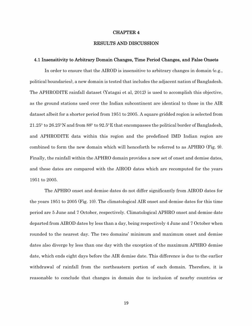
dataset albeit for a shorter period from 1951 to 2005. A square gridded region is selected from

21.25 to 26.25N and from 88 to 92.5E that encompasses the political border of Bangladesh,

and APHRODITE data within this region and the predefined IMD Indian region are

combined to form the new domain which will henceforth be referred to as APHRO (Fig. 9).

Finally, the rainfall within the APHRO domain provides a new set of onset and demise dates,

and these dates are compared with the AIROD dates which are recomputed for the years

1951 to 2005.

The APHRO onset and demise dates do not differ significantly from AIROD dates for

the years 1951 to 2005 (Fig. 10). The climatological AIR onset and demise dates for this time

period are 5 June and 7 October, respectively. Climatological APHRO onset and demise date

departed from AIROD dates by less than a day, being respectively 4 June and 7 October when

rounded to the nearest day. The two domains’ minimum and maximum onset and demise

dates also diverge by less than one day with the exception of the maximum APHRO demise

date, which ends eight days before the AIR demise date. This difference is due to the earlier

withdrawal of rainfall from the northeastern portion of each domain. Therefore, it is

reasonable to conclude that changes in domain due to inclusion of nearby countries or

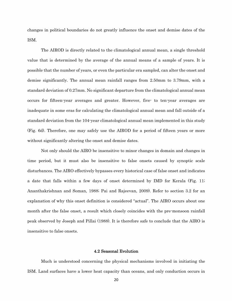
20

changes in political boundaries do not greatly influence the onset and demise dates of the

ISM.

The AIROD is directly related to the climatological annual mean, a single threshold

value that is determined by the average of the annual means of a sample of years. It is

possible that the number of years, or even the particular era sampled, can alter the onset and

demise significantly. The annual mean rainfall ranges from 2.50mm to 3.79mm, with a

standard deviation of 0.27mm. No significant departure from the climatological annual mean

occurs for fifteen-year averages and greater. However, five- to ten-year averages are

inadequate in some eras for calculating the climatological annual mean and fall outside of a

standard deviation from the 104-year climatological annual mean implemented in this study

(Fig. 6d). Therefore, one may safely use the AIROD for a period of fifteen years or more

without significantly altering the onset and demise dates.

Not only should the AIRO be insensitive to minor changes in domain and changes in

time period, but it must also be insensitive to false onsets caused by synoptic scale

disturbances. The AIRO effectively bypasses every historical case of false onset and indicates

a date that falls within a few days of onset determined by IMD for Kerala (Fig. 11;

Ananthakrishnan and Soman, 1988; Pai and Rajeevan, 2009). Refer to section 3.2 for an

explanation of why this onset definition is considered “actual”. The AIRO occurs about one

month after the false onset, a result which closely coincides with the pre-monsoon rainfall

peak observed by Joseph and Pillai (1988). It is therefore safe to conclude that the AIRO is

insensitive to false onsets.

4.2 Seasonal Evolution

Much is understood concerning the physical mechanisms involved in initiating the

ISM. Land surfaces have a lower heat capacity than oceans, and only conduction occurs in

21

soil whereas heat is dispersed through both conduction and convection in water. This

difference allows for more rapid heating (or cooling in the absence of a heat source) over land

than over water. The land is therefore much colder in boreal winter due to radiative cooling

compared to oceans which retain some of the previous summer’s radiation. As spring gives

way to summer, incoming solar radiation intensifies at increasingly higher latitudes. Not

only are there large land masses farther north of the equator, but the Tibetan Plateau is a

location of very high altitude. Since the atmosphere becomes cooler at higher altitudes, but

land effectively heats (cools) the overlying atmospheric column in the presence (absence) of

solar radiation, this plateau acts as an elevated heat source during the summer (Wu and

Zhang, 1998). At a certain point during the year, the meridional temperature gradient

produced by the land-ocean temperature contrast and exacerbated by the Tibetan Plateau

reverses sign, becoming negative instead of positive (Yanai et al., 1992; Hsu et al., 1999).

As the atmosphere above land experiences anomalous heating relative to that above

ocean, the atmospheric column expands and its density decreases as mass is displaced by

divergence at the tropopause. This tropospheric expansion and contemporaneous upper-level

divergence results in an anomalously low surface pressure over the Indian subcontinent. The

pressure gradient between the land and the surrounding ocean increases and is partially

offset by the Coriolis, centrifugal, and viscous forces that slow incoming winds and turn them

to the right in the Northern Hemisphere. Therefore, winds flow cyclonically inward to

equalize the pressure difference and restore the force imbalance (Rao, 1976; Hsu et al, 1999).

Prior to onset, low-level wind near the equator is westerly in the Southern

Hemisphere and easterly in the Northern Hemisphere. The aforementioned large-scale

cyclonic circulation over the Indian subcontinent in combination with counterclockwise

rotation about the Mascarene High in the Southern Hemisphere cause the low-level wind

direction near the equator in both hemispheres to reverse and intensify, especially off the

22

Somali coast (Rao, 1976; Webster and Yan, 1992; Soman and Kumar, 1993; Lau et al., 1998;

Goswami et al., 1999; Hsu et al., 1999). The ocean currents averaged over the mixed layer of

the ocean, known as the Ekman current, flow to the right (left) of the surface wind in the

Northern (Southern) Hemisphere due to the influence of the wind-induced stress at the

surface and the competing Coriolis and turbulent drag forces at various depths (Fig. 12;

Ekman, 1905). Therefore, a reversal of wind across the Indian Ocean forces a basin-wide

reversal of the Ekman current and its related heat transport (Fig. 13; Loschnigg and Webster,

2000).

Frictional convergence occurs as moisture-laden surface winds transition from the

lower-friction Arabian Sea and Bay of Bengal to the rougher land surface of the southern tip

and northeastern region of the Indian subcontinent, hence contributing to excess moisture

over Kerala and the seven sister states (Fig. 1). Numerous processes assists this surplus of

precipitable moisture. Diabatic heating over land increases buoyancy and causes mixing of

warm, dry air above the land with cooler, moist air from the ocean (Hsu et al., 1999). This

convergent air is then orographically lifted on the windward side of the Western Ghats

mountain range in the south and the Himalayan Mountains in the northeast. This sudden

availability of instability, moisture, and lift results in deep moist convection and intense

rainfall over Kerala and the seven sister states (Ananthakrishnan and Soman, 1988; Soman

and Kumar, 1993; Lau et al., 1998; Goswami and Gouda, 2010). Meanwhile, a more steady

increase in precipitation takes place in central India as moisture converges due to the large-

scale cyclonic circulation previously discussed.

It is clear that a seasonally varying land-ocean temperature contrast influences large-

scale atmospheric circulations, which in turn reverses oceanic circulations and results in

sudden and severe regional precipitation. The AIROD captures the seasonal evolution of

23

these large-scale atmospheric and oceanic processes and in so doing reveals its intrinsic

relationship with the physical mechanisms that initiate the onset and demise of the ISM.

4.2.1 The Land-Ocean Temperature Contrast

Increased heating of the Tibetan Plateau and, to a lesser extent, the entire continental

landmass is evident leading up to the onset of the ISM (Wu and Zhang, 1998). An increase of

300hPa temperature first begins in the East Asian monsoon region and the Bay of Bengal a

month before the onset of the ISM. Roughly five days before the AIRO, intensified heating

over the region surrounding the seven sister states expands to the east and west, resulting

in higher temperatures to the north than nearer the equator (Fig. 14). This relatively high

northerly upper level temperature persists until about twenty days before the AIRD when it

begins to contract towards the Himalayan foothills and withdraw to the southeast (Fig. 15).

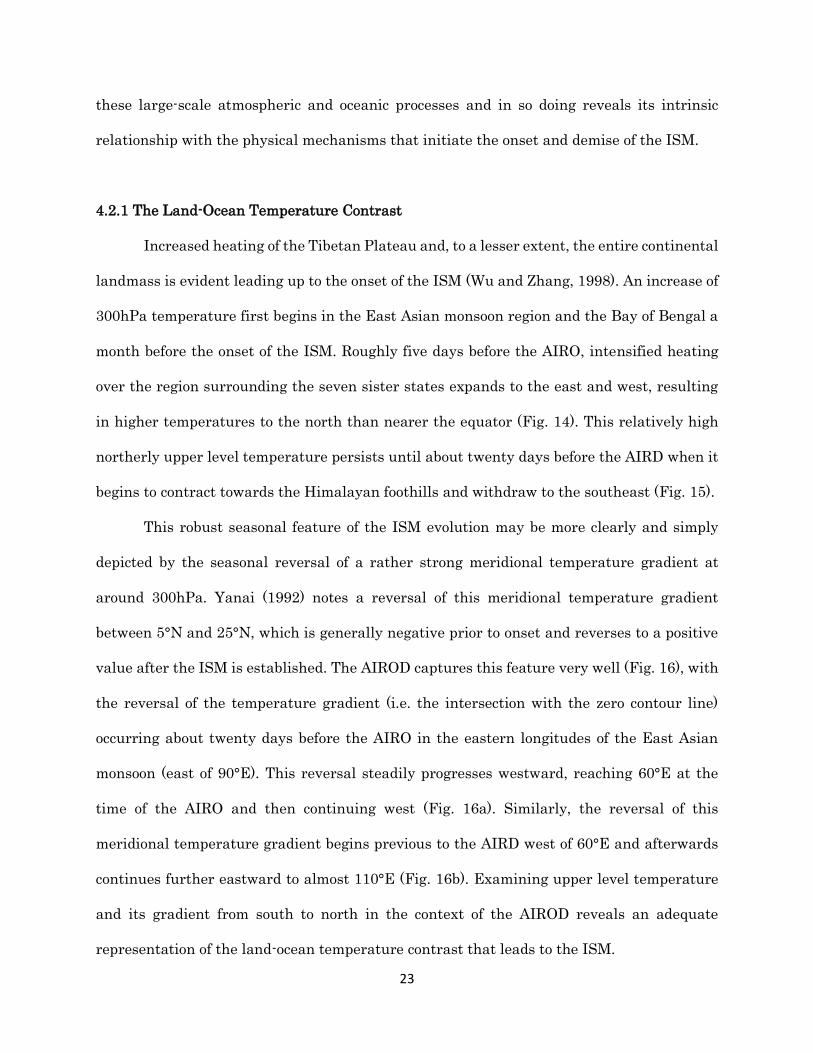
This robust seasonal feature of the ISM evolution may be more clearly and simply

depicted by the seasonal reversal of a rather strong meridional temperature gradient at

around 300hPa. Yanai (1992) notes a reversal of this meridional temperature gradient

between 5°N and 25°N, which is generally negative prior to onset and reverses to a positive

value after the ISM is established. The AIROD captures this feature very well (Fig. 16), with

the reversal of the temperature gradient (i.e. the intersection with the zero contour line)

occurring about twenty days before the AIRO in the eastern longitudes of the East Asian

monsoon (east of 90°E). This reversal steadily progresses westward, reaching 60°E at the

time of the AIRO and then continuing west (Fig. 16a). Similarly, the reversal of this

meridional temperature gradient begins previous to the AIRD west of 60°E and afterwards

continues further eastward to almost 110°E (Fig. 16b). Examining upper level temperature

and its gradient from south to north in the context of the AIROD reveals an adequate

representation of the land-ocean temperature contrast that leads to the ISM.

24

4.2.2 Large-Scale Atmospheric Circulation Reversal

The reversal of low-level winds off the Somali coast is of paramount importance to

accurately represent as the monsoon is technically defined by this seasonal shift of prevailing

wind direction. Upper and lower level winds, and their combined vertical wind shear, reverse

and intensify around the time of the onset of the ISM (Webster and Yang, 1992; Lau et al.,

1998; Goswami et al., 1999; Hsu et al., 1999). Fig. 17 displays constantly vigorous 850hPa to

200hPa vertical wind shear in the midlatitudes as a result of the upper level jetstream that

shifts further north as the AIRO approaches. What is of most importance concerning the

mechanisms associated with the AIRO, however, is the growth of vertical wind shear in the

typically shearless tropical environment. This shear first begins to develop in the southern

Bay of Bengal about fifteen days before the AIRO, and by the AIRO the vertical wind shear

over the southern Arabian Sea off the coast of Somalia doubles in magnitude (Fig. 17). This

vertical wind shear continues to intensify and extend toward the Indian peninsula as the

ISM progresses until a little over a month before the AIRD. By the AIRD, vertical wind shear

is weakened and its attendant winds are weakened in the tropics, while the upper level

jetstream in the midlatitudes intensifies and shifts further south as boreal winter approaches

(Fig. 18).

Kinetic energy of 850hPa winds dramatically increase as a direct consequence of the

reversal and subsequent increase of low-level winds (Krishnamurti and Ramanathan, 1982).

Krishnamurti and Ramanathan (1982) observes more than an order of magnitude increase

in zonal kinetic energy over a period of a week for the year 1979 from 50° to 70°E and 4°S to

20°N. A 104-year composite analysis does not show as drastic a change (Figs. 19 and 20). This

suggests that the year 1979 had an anomalously large increase in kinetic energy and that

such limited sampling improperly magnified the expected magnitude of increase in low-level

kinetic energy. A new region of interest is selected from 50 to 75° and 5 to 20°N to most

25

adequately represent the changes in total kinetic energy of 850hPa winds during the seasonal

evolution of the ISM. Prior to onset, kinetic energy is marginal and remains below 75m2s-2.

Kinetic energy suddenly doubles during onset to 150m2s-2, and then doubles again as the ISM

progresses (Fig. 19). Kinetic energy changes more slowly during withdrawal of the ISM, and

by the AIRD has decreased to less than 50m2s-2 (Fig. 20). Thus, while the increase in low-

level kinetic energy is not as dramatic as is anticipated by previous studies, its evolution

remains quite sudden and its characteristics are clear. These two wind-based variables show

that the AIROD captures the reversal and subsequent intensification of the atmospheric

circulation well.

4.2.3 Large-Scale Oceanic Circulation Reversal

A reversal in Ekman heat transport in the Indian Ocean accompanies the reversal in

atmospheric circulation preceding the onset of the ISM. Loschnigg and Webster (2000) notes

such a dramatic reversal from northward to southward Ekman heat transport that it roughly

balances the northward atmospheric heat transport. The pattern of reversal of basin-wide,

zonally-averaged meridional ocean heat transport given in previous literature (Chirokova

and Webster, 2006) is replicated by the AIROD (Fig. 21). Below about 15°S, meridional heat

transport remains southward throughout most of the year. The reversal from northward to

southward meridional heat transport begins at about 12°S, and this reversal rapidly

propagates northward about twenty to forty days before the AIRO up to around 10°N. The

most sudden reversal and subsequent intensification of southward transport seems to take

place here, and by the AIRO southward heat transport is occurring at all but the most

northern latitudes of the Indian Ocean (Fig. 21a). Within roughly three months, meridional

heat transport once again reverse from southward to northward transport, beginning in the

26

northern latitudes and reaching 10°N by the AIRD. This reversal continues at a slower rate

into the Southern Hemisphere after the AIRD (Fig. 21b).

A few interesting characteristics of meridional ocean heat transport should be

mentioned. First, 10° to 15°S experiences the greatest southward heat transport in the

southern portion of the Indian Ocean, which is in agreement with previous research

(Chirokova and Webster, 2006; Sun et al., 2014). There exists the most sudden and strong

gradient in meridional heat transport at about 8° to 10°N, where reversal occurs a little less

than twenty days before the AIRO. Both of these are two examples of the multiple striations

in meridional heat transport apparent throughout the Indian Ocean (Fig. 21). This

inhomogeneous transport results from the competition between boundary currents and the

basin-wide Ekman transport. Higher values of meridional heat transport are observed, as

stated above at 10° to 15°S and 8° to 10°N. The former is the latitudinal domain of the

Mozambique and Southeast Madagascar Currents, which continually flow to the south. The

latter is the location of the Great Whirl which produces roughly balanced meridional

transport (Beal and Donohue, 2013, Akuetevi et al., 2016). These phenomena, especially the

currents to the south, positively reinforce the basin-wide southward Ekman transport

immediately before and during the ISM, thus generating greater southward meridional heat

transport. Conversely, the East African Coastal Current (around 10°S to the equator) flows

consistently northward throughout the year, thus opposing basin-wide Ekman transport

preceding and during the ISM and causing weaker southward meridional heat transport (Fig.

21a). The Somali Current is unique in that it is the only ocean current that experiences an

annual reversal, flowing northward in the boreal summer and southward in the boreal winter

(Beal and Donohue, 2013). This current opposes the flow of Ekman transport before, during,

and after the ISM, therefore weakening southward meridional heat transport during the ISM

and weakening northward meridional heat transport at other times of the year (Fig. 21a). All

27

of these interactions appear during the seasonal evolution of meridional heat transport based

on the AIROD.

Another interesting characteristic of meridional heat transport is the diagonal lines

of alternating maximum and minimum transport across the equator (Fig. 21). This

phenomena is explained by the Rossby duct hypothesis (Sahami, 2003). Pairs of Rossby waves

straddling the equator form a wave train between the southward Ekman transport that

begins at roughly 6°S and 6°N. Ekman transport becomes infinitesimal near the equator as

the Coriolis force weakens and ultimately reverses. The Rossby wave structures that span

this equatorial region where Ekman flow is no longer valid allow continuous flow across the

equator through the ducts displayed in Fig. 22. The southward flow within the antisymmetric

structure of the waves is enhanced by the steady southward flow which overlaps the poleward

edges of the equatorial wave guide, thus resulting in regions of enhanced southward heat

transport near the equator (Figs. 21 and 22; Sahami, 2003).

Finally, for reasons that are unclear, this study’s values are almost exactly an order

of magnitude smaller than that of previous studies (a maximum of 0.3PW compared to a

maximum of 2.5PW) despite the pattern of meridional heat transport being nearly identical

(Chirokova and Webster, 2006). This discrepancy may not be attributed to the influence of

boundary currents because separate calculations were completed excluding the boundary

which obtained similar magnitudes. Furthermore, the problem is not a result of spatial

resolution, since a recent research with 0.5° resolution (identical to this study) derives similar

values as previous research (Sun et al., 2014). It is possible that either CFSR or other models

(e.g., two-and-a-half-layer Indian Ocean model; SODA) are unable to accurately resolve the

strength of ocean currents and therefore inadequately represent meridional heat transport.

This seems unlikely, however, given the striking similarity in the pattern of meridional heat

transport between the different models. Other reasons for the difference in magnitude

28

include the difference in time step or the difference in depth over which transport is

integrated. Chirokova and Webster (2006) compute meridional heat transport in five-day

intervals, which is insufficient for determining the date of onset and may lead to different

values than the previous study. A difference as drastic as an order of magnitude, however,

could not result from this difference in time step. Previous research integrates over the top

500 meters (Chirokova and Webster, 2006) or entire depth (Sun et al., 2014) of the Indian

Ocean, whereas the current study only integrates the top 105 meters known as the mixed

layer. Deeper sampling could result in an increase in meridional heat transport (i.e.

additional layers provides a greater value) or, if too deep, a potential decrease in transport

(i.e. opposing undercurrents are also included in integration). That said, multiple depths

were attempted in this study that altered the pattern of the meridional heat transport more

than its magnitude. In conclusion, while meridional heat transport seems to provide advance

warning for the AIROD, it must be further scrutinized to understand the discrepancies

involved.

4.2.4 Moisture Convergence and Subsequent Precipitation

The AIROD is based upon rainfall, so it is expected and of highest priority that the

seasonal evolution of moisture-based variables are well represented. Vertically integrated

moisture flux convergence begins to increase in an arc to the south and east of the Indian

subcontinent about fifteen days prior to the AIRO due to the large-scale cyclonic circulation

about the landmass. Meanwhile, divergence exists over the central Arabian Sea and southern

India. By the AIRO, frictional convergence over the southern tip of India and over the seven

sister states generates a maximum in moisture convergence. This convergence arises from

the shift from relatively frictionless ocean to the rough land surface and mountain ranges.

About fifteen days later, large-scale convergence causes moisture to congregate over central

29

India (Fig. 23). This moisture convergence persists only over the Himalayan foothills by the

AIRD, at which point there is widespread divergence over land and convergence over the Bay

of Bengal and the South China Sea (Fig. 24). This southwestward withdrawal of moisture

provides the environmental setup necessary for the Australian monsoon.

A similar evolution may be seen for precipitable water. Moderate values (45-50kgm-2)

reside only in the southern Bay of Bengal about a month before the AIRO. These moderate

values then begin to expand and increase, first over far eastern Asia, followed by the northern

Arabian Sea and finally over the southern Arabian Sea and the seven sister states to the

north. At AIRO, precipitable water dramatically intensifies discreetly at the coast of Kerala

and over the seven sister states. After onset, high values (55-60kgm-2) of precipitable water

progress over central India, with the highest values (60-65kgm-2) remaining over the

Himalayan foothills (Fig. 25). As the AIRD approaches, higher values of precipitable water

withdraw eastward and are constrained to the Bay of Bengal (Fig. 26). This evolution is

nearly identical to vertically integrated moisture flux convergence since a convergence of

moisture leads to a localized higher concentration of moisture, or precipitable water. The rain

shadow to the east of the Western Ghats in southern India (which is also captured in rainfall

composites) is more clearly visible as a minimum in precipitable water, however (Fig. 25).

The most dramatic change captured by the AIROD is that of gridded rainfall. The

Indian subcontinent is devoid of even light (2-10mmday-1) rainfall except for over the seven

sister states, which are influenced by the Asian monsoon and thus exhibit a rather steady

moderate (10-20mmday-1) rainfall up to two months in advance of the AIRO. On the AIRO

date, rainfall dramatically increases (20-30mmday-1) in Kerala and the seven sister states

with a light (2-8mm) increase beginning in south and east India. As the ISM progresses,

central India sees a major increase (10-20mmday-1) in rainfall that then extends to the

northwest. Meanwhile, the seen sister states, and to a greater extent the southwest Indian

30

coast, experience severe (>30mmday-1) rainfall (Fig. 27). This heavy precipitation across the

Indian subcontinent persists until about 45 days before the AIRD when rainfall begins to

slowly weaken in all regions. Withdrawal begins in the northeast about 25 days before the

AIRD. This gradual withdrawal and weakening precipitation abruptly accelerates

immediately before the AIRD, leaving only light (2-10mm) rainfall in India. This rainfall

slightly increases within a few days and persists in southeast India for at least two months

as the Indian winter monsoon arrives (Fig. 28).

4.3 Interannual Variability

The AIROD has been shown to adequately represent the seasonal evolution of the ISM

and changes in its related large-scale atmospheric and oceanic phenomena. The interannual

variability of the AIROD and its associated large-scale variables is assessed to determine

how one varies with respect to the other. Possible causal relationships are also discussed by

using the physical mechanisms observed during the seasonal evolution previously presented

and using lead and lag relationships.

4.3.1 Features of the Indian Summer Monsoon

Before analyzing the interannual variability of large-scale atmospheric and oceanic

variables, one must understand how certain ISM features are interrelated. Five features are

of particular interest: AIRO, AIRD, season length, total seasonal AIR, and mean seasonal

AIR. While the AIRO and AIRD are not significantly correlated with each other (-0.12), both

are highly correlated with season length (-0.67 and 0.82, respectively; Table 6). This

relationship indicates that an early (late) AIRO date and a late (early) AIRD date by

definition result in a longer (shorter) length of the ISM. Furthermore, the AIRO and AIRD

are well correlated with total seasonal AIR (-0.43 and 0.61, respectively), showing that an

31

early (late) AIRO date and a late (early) AIRD date also result in greater seasonal rainfall

averaged over India (Table 6). This could be a direct result of increased season length, or of

increased rain rate at the beginning or end of the ISM. However, the sign of correlation

coefficient switches for the AIRO and AIRD with mean seasonal AIR (0.27 and -0.24,

respectively) compared to total seasonal AIR, which insinuates that the effect of season

length on total seasonal AIR is more significant than that of rain rate (Tables 6 and 7).

Caution is recommended in interpretation of these correlations, however, as it is possible that

cross-correlation has caused inappropriate inflation of values. This effect could arise from the

inherent noisiness of rainfall data, but cannot be removed from results due to the difficult

task of distinguishing noise from annual variability.

Total seasonal rainfall variability dominates in different locations for changes in

AIRO date and AIRD date. An early (late) AIRO date suggests a higher probability (� � =− . ) of increased (decreased) seasonal rainfall particularly in the seven sister states,

although central and southern India also weakly retain this relationship (Fig. 29a). A late

(early) AIRD date, on the other hand, suggests an even greater probability (� � = . ) of

increased (decreased) seasonal rainfall predominantly in southeast India, but to a lesser

extent throughout the remainder of the Indian subcontinent (Fig. 29b). The reason for this

discrepancy of location of increased seasonal rainfall is rather simple. An early AIRO date

implies an increase in rainfall compared to climatology near the beginning of the season, and

the opposite may also be argued concerning a late AIRO date. ISM rainfall commences over

Kerala and the seven sister states, so this early-season anomalous rainfall should influence

the total seasonal rainfall most greatly in these regions. Likewise, ISM rainfall reaches its

final point of withdrawal in southeast India, so a late (early) AIRD date should result in

32

increased (decreased) late-season rainfall relative to climatology and consequently increased

(decreased) total seasonal rainfall at this location.

4.3.2 Temperature

Upper level temperature anomalies vary as the timing of the AIROD changes. The

300hPa meridional temperature gradient between 5°N and 25°N reveals a significantly

negative correlation (� � = − . ) from 40°E to 70°E beginning fifteen days before the AIRO

that extends eastward to 90°E at AIRO and persists for another twenty days (Fig. 30a). That

is, an early (late) AIRO date is associated with an increased (decreased) meridional

temperature gradient anomaly relative to climatological values fifteen days before to twenty

days afterwards. An inverse relationship exists between the AIRD and the upper level

meridional temperature gradient (� � = . ), with an early (late) AIRD date often

associated with a decreased (increased) meridional temperature gradient anomaly beginning

five days before at about 80°E and continuing until about five days afterwards at about 60°E

(Fig. 30b). A climatologically anomalous meridional temperature gradient observed to persist

for roughly ten to fifteen days may indicate the timing of the AIRO.

The zonal progression of this anomaly of temperature difference between latitudes

can be further explored by observing the spatial relationship between the AIROD and 300hPa

temperature itself. The anomalous increase (decrease) in upper level temperature begins

about ten days prior to an early (late) AIRO over the Arabian and Thar deserts to the west,

and then slowly progresses across the Arabian Sea and into northern India five days after

the AIRO (Fig. 31). The opposite progression of temperature anomalies takes place at the end

of the ISM, with AIRD date anomalies positively correlated with temperature anomalies five

days before over northern India to five days after over the western deserts (Fig. 32). It should

33

be noted that while the maximum upper level temperatures occur in northeast India (Fig.

14), the anomalous relationship indicating the arrival of the AIROD is far west of this

maximum.

4.3.3 Wind

Less can be said about the relationship between 850hPa to 200hPa vertical wind shear

and the AIROD because of the noisiness of observations of vertical wind shear and the

possibly strong influence of intraseasonal variability contaminating the analysis. This

noisiness may in part be a result of sampling 200hPa winds, which are not represented with

great accuracy by the surface-assimilated ERA-20C (Poli et al., 2013). However, a general

conclusion can be made that an early (late) AIRO date would occur shortly after an early

(late) establishment of the large-scale atmospheric circulation about the Indian subcontinent.

This relationship is manifested as negative correlations (� � = − . ) extending across the

Indian Ocean at the southern tip of the subcontinent and positive correlations (� � = . )

extending across northern India and the bordering nations around the AIRO (Fig. 33). These

correlations then flip signs in the days before and after the AIRD (Fig. 34), insinuating that

an early (late) AIRD date corresponds to an early (late) withdrawal of the large-scale

atmospheric circulation about the Indian subcontinent.

The variability of kinetic energy of 850hPa winds, however, is more clearly related to

the timing of the AIROD. Beginning fifteen days before the AIRO, there appears an

anomalous increase (decrease) in low-level kinetic energy off the Somali Coast for an early

(late) AIRO date (� � = − . ). As the AIRO approaches, this anomaly shifts eastward across

the Arabian Sea, all the while remaining centered just north of 10°N (Fig. 35). A rather

similar process develops during and after the AIRD, with a positive correlation (� � = . )

34

centered just south of 10°N and slowly progressing westward across the Arabian Sea (Fig.

36). This variability of the kinetic energy is useful to monitor as it exhibits a highly

concentrated and easily recognized anomaly well in advance of the AIRO.

4.3.4 Oceanic Phenomena

Not much may be deduced from the correlation of AIROD dates with meridional ocean

heat transport (Fig. 37). The noisiness and wave-like patterns may be result of the slow

response of the ocean compared to the atmosphere and the production of westward-

propagating Rossby waves. Due to these complications, no reasonable conclusions may be

drawn from this relationship.

Teleconnections exist between AIRO date variability and the preceding December-

February (DJF) averaged sea surface temperature (SST) variability. Three such

teleconnections dominate. First, cool (warm) DJF SSTs in the equatorial Pacific Ocean

indicate the possibility (� � ≈ . ) of an early (late) AIRO date (Fig. 38). That is, La Niñas

(El Niños) often precede early (late) AIRO dates. Joseph et al. (1994) supports this claim,

noting that most significantly delayed onsets occur after an El Niño. Second, warm (cool) DJF

SSTs in the Mediterranean Sea significantly correspond (� � = − . ) to a subsequent early

(late) AIRO date (Fig. 38). While previous research has studied the relationship between

Mediterranean SST and Indian seasonal rainfall variability (Fontaine et al., 2011), no

research has analyzed the relationship between said SST and onset date variability

discovered herein. Finally, there is an oceanic phenomena located in the southern Pacific

Ocean called the South Pacific Dipole (SPD) (Guan et al., 2013). When DJF SSTs are cool

(warm) in the eastern SPD and warm (cool) in the western SPD, an early (late) AIRO date is

anticipated (� � = . ; Fig. 38). That is, a westward (eastward) DJF SST gradient across

35

the SPD suggests an early (late) AIRO date the following boreal spring or summer. These

DJF SST teleconnections can be monitored to provide a tentative estimate of the timing of

the following AIRO date.

The relationship of ENSO with ISM features may be analyzed in greater detail by

correlating monthly Niño 3.4 SSTs with AIRO, AIRD, total seasonal AIR, and June-

September (JJAS) All-India Monsoon Rainfall (AIMR, a commonly used index for

determining interannual ISM variability; Parthasarathy and Pant, 1985). The relationship

of Niño 3.4 SST with total seasonal AIR and AIMR is much more robust than its relationship

with AIRO and AIRD (Fig. 39). In fact, seasonal AIR and AIMR account for over 35% of the

variance in the subsequent ENSO mode (� ≈ − . ). Thus, a wet (dry) ISM offers greater

confidence that there will follow a La Niña (El Niño). ENSO and total monsoon rainfall are

linked by the westerly wind bursts over the tropical Pacific Ocean. Kirtman and Shukla

(2000) show that a weak (strong) monsoon leads to a weakening (strengthening) of the trade

winds, which in turn make a warm (cold) ENSO warmer (colder) approximately six months

later. Note also that the total seasonal AIR computed from the AIROD is very similar to the

JJAS AIMR, but it has higher values on average due to sampling before or after the JJAS

season (Fig. 40). Because the AIROD is intricately linked to large-scale phenomena which

influence the evolution of the ISM, total seasonal AIR’s flexibility likewise offers a more

physically-based depiction of the ISM than the static JJAS AIMR index does.

4.3.5 Moisture

Moisture-based variables also experience interannual variability in relationship with

the timing of the AIROD. Because vertically integrated moisture flux convergence is itself a

noisy variable as supplied by ERA-20C, its interannual variability is also quite complex. All

36

that can be confidently said about its relation to the AIRO is that there exists an increased

(decreased) anomaly of moisture convergence on the southwest Indian coast and in the upper

Bay of Bengal about fifteen days before and after an early (late) AIRO date, although the

exact location of this anomaly likely shifts significantly from year to year (Fig. 41). Even less

may be said concerning its interaction with the timing of the AIRD date (Fig. 42).

Precipitable water reveals a much clearer negative (positive) correlation (� � =− . ; � � = . ) with the AIRO (AIRD) date. There exists an anomalous increase

(decrease) in precipitable water compared to climatological values about ten days before an

early (late) AIRO date centered over the northeastern Arabian Sea, which then drifts over

north-central India by the AIRO and continues over the northern Bay of Bengal a few days

later. This excess (deficit) in precipitable water over north-central India during an early (late)

AIRO is balanced by a deficit (excess) in the surrounding domain (Fig. 43). Conversely, an

anomalous increase (decrease) in precipitable water over central India exists five days before

and after a late (early) AIRD date (Fig. 44).

This relationship between precipitable water and the AIROD is nearly replicated with

rainfall. By first observing the relationship between spatially-averaged AIR and the AIRO, a

significantly negative correlation is noticed from a little more than ten days before AIRO to

a little less than ten days after, with a minimum (� � = − . ) at AIRO (Fig. 45a). This

means that an anomalous increase (decrease) in AIR is associated with an anomalously early

(late) AIRO date. This is expected, for the AIROD is based upon AIR. Consequently, a positive

(� � = . ) correlation between AIR and the AIRD is observed roughly five days before to

just over ten days after the AIRD (Fig. 45b). Note that correlations become insignificant

outside of this range. Therefore, a portion of early and late seasonal rainfall variability may

be known if the AIROD variability is accurately predicted. The relationship between gridded

37

rainfall and the AIROD reveals that these negative (positive) anomalies, which are associated

with the AIRO (AIRD), occur predominantly over central India. Increased (decreased) rainfall

occurs in central India and along the central western coast prior to an early (late) AIRO date

and after a late (early) AIRD date (Figs. 46 and 47). While the location of anomalous rainfall

and precipitable water may be surprising considering that the greatest moisture exists over

Kerala and the seven sister states (Figs. 25-28), this result agrees with many previous studies

that have found central India to adequately represent variability across the entire Indian

subcontinent with respect to pressure, temperature, and rainfall anomalies (Hastenrath and

Rosen, 1983; Parthasarathy et al., 1990; Kumar et al., 1995). For this reason, anomalous

precipitable water and especially rainfall may be monitored prior to the AIRO to assist in

determination of its timing.

38

CHAPTER 5

CONCLUSION

The newly proposed All-India rainfall onset and demise (AIROD), an AIR-based index

that objectively determines the onset and demise dates of the Indian summer monsoon (ISM),

has been intricately examined. It is very simple, being based exclusively on rainfall averaged

over all of India, a variable which has been reliably observed for over a century and which

allows those outside of the scientific community to perceive ISM variability more easily.

Minimal resources would be required to supplement existing methods of monitoring the onset

of the ISM with the AIROD because of its very simple computation and its foundation upon

a rainfall dataset which is already monitored by the IMD. Furthermore, AIROD successfully

avoids all recorded false onsets and provides an onset date that closely parallels IMD onset

definitions.

The AIROD seems to be the most representative onset index proposed to date and is

intricately related to changes in large-scale phenomena that characterize the ISM. This index

is verified with the seasonal evolution of other dynamic (i.e. wind-based) and thermodynamic

(i.e. temperature- and moisture-based) variables of the ISM and is shown to be consistent

with their evolution. The zonal (meridional) progression of the reversal of the 300hPa

meridional temperature gradient (meridional ocean heat transport) may be detected almost

three weeks in advance of the onset, providing advanced warning of its timing. Moisture-

based features such as vertically integrated moisture flux convergence, precipitable water,

and rainfall are seen to dramatically increase (decrease) over Kerala and the seven sister

states prior to the onset (demise) and subsequently over central India. Wind-based features

such as 850hPa to 200hPa vertical wind shear and kinetic energy of the 850hPa winds also

increase rapidly over a few days off the Somali coast and extend eastward across the Arabian

39

Sea as the onset approaches. Similarly, 300hPa temperature is also seen to increase across

the domain, but most greatly over northeast India prior to onset.

Interannual variability of large-scale phenomena as a result of the timing of the

AIROD is also assessed. Total seasonal rainfall anomalies are captured by AIROD anomalies,

with early (late) onset and late (early) demise resulting in an increase (decrease) of seasonal

rainfall. This relationship indicates that close monitoring of the onset can provide additional

information about the development of an anomalous ISM season. In addition, seasonal

rainfall seems to be a good predictor of a subsequent ENSO mode, with a wet (dry) ISM

season preceding a La Niña (El Niño). Furthermore, the flexible nature of total seasonal AIR,

which is computed using the AIROD, offers a more accurate, physically-based depiction of

the interannual variability of the ISM than does the commonly-used JJAS All-India monsoon

rainfall (AIMR) index. DJF SST teleconnections also exist in relation to the timing of onset,

providing weak preliminary estimates almost half a year in advance. Two other potentially

useful indicators of the timing of onset are the zonal progression of the anomaly of kinetic

energy of 850hPa winds fifteen days prior, and the anomalous central Indian rainfall ten

days prior, to onset.

Research is currently underway to define local and regional transition dates that

would contribute to the currently-defined AIROD but offer a more useful application for end

users. The predictability of the AIROD using weather and climate models is also being

studied. ISM variability on longer than the interannual time scale will also be examined

using Empirical Ensemble Mode Decomposition (EEMD) analysis (Wu and Huang, 2009).

Other interesting future research may include application of the index to other variables with

strong seasonal cycles. One could determine annual onset dates each based on a different

large-scale variable, and then search for a consistent order of these dates. As each onset date

is triggered in a given year, forecasters would then be able to narrow their forecast for the

40

AIR-based onset date, which occurs last and represents the arrival of the ISM. Finally,

zonally-integrated meridional ocean heat transport must be investigated in greater detail

both to determine the cause of the order-of-magnitude discrepancy in this study and to better

understand the influence of boundary currents upon basin-wide transport.

41

APPENDIX A

TABLES

Source Variables Domain Large-scale transition

Rao (1976) Surface pressure and wind

Bay of Bengal:

north of 18N

Monsoon depressions (2-3 closed isobars at 2hPa

intervals over 5 square grid; surface winds 17-33kts)

Krishnamurti and Ramanathan (1982)

Zonal wind Arabian Sea:

50-70E, 4S-20N

850hPa kinetic energy of zonal wind increases by order of magnitude

Murakami and Nakazawa (1985)

Outgoing longwave radiation (OLR) and wind

Global Asymmetric component of OLR reverses and 200hPa velocity potential divergence transitions from Southern to Northern Hemisphere

Ananthakrishnan and Soman (1988)

Rainfall Kerala, India:

815’N-1250’N

Rainfall suddenly shifts from light (<10mmday-1) to strong (>10mmday-1) regime

Webster and Yang (1992)

Zonal wind 40-110E, 0-20N

850-200hPa vertical wind shear of zonal winds reverses

Yanai et al. (1992)

Temperature 40-130E, 0-50N

500-200hPa layer-mean meridional temperature

gradient from 5N to 25N reverses

Soman and Kumar (1993)

Rainfall, relative humidity (RH), vertically integrated zonal moisture transport (VIZMT), wind, and OLR

India (23 scattered stations)

Rainfall, RH, and VIZMT sharply increase, upper-tropospheric winds change strength and transition north, and OLR rapidly decreases

Table 1. Large-scale atmospheric and oceanic changes associated with onset from previous literature.

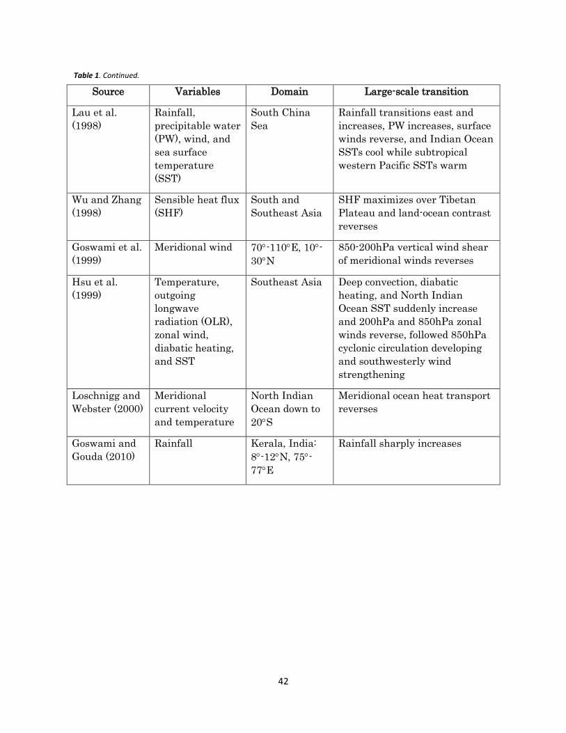
42

Source Variables Domain Large-scale transition

Lau et al. (1998)

Rainfall, precipitable water (PW), wind, and sea surface temperature (SST)

South China Sea

Rainfall transitions east and increases, PW increases, surface winds reverse, and Indian Ocean SSTs cool while subtropical western Pacific SSTs warm

Wu and Zhang (1998)

Sensible heat flux (SHF)

South and Southeast Asia

SHF maximizes over Tibetan Plateau and land-ocean contrast reverses

Goswami et al. (1999)

Meridional wind 70-110E, 10-30N

850-200hPa vertical wind shear of meridional winds reverses

Hsu et al. (1999)

Temperature, outgoing longwave radiation (OLR), zonal wind, diabatic heating, and SST

Southeast Asia Deep convection, diabatic heating, and North Indian Ocean SST suddenly increase and 200hPa and 850hPa zonal winds reverse, followed 850hPa cyclonic circulation developing and southwesterly wind strengthening

Loschnigg and Webster (2000)

Meridional current velocity and temperature

North Indian Ocean down to

20S

Meridional ocean heat transport reverses

Goswami and Gouda (2010)

Rainfall Kerala, India:

8-12N, 75-77E

Rainfall sharply increases

Table 1. Continued.

43

Source Variables Domain Onset Index

Ananthakrishnan et al. (1968)

Rainfall Kerala (seven stations)

- After 10 May, second in a period of two days when five of seven stations receive >1mm of rainfall

Ramage (1971) Wind Global - Prevailing wind direction shifts by at least 120 and persists for at least 40% of the time in January and July - Mean wind exceeds 3ms-1 in January or July - Fewer than one cyclone-anticyclone alternation occurs every two years in January or July in a 5 rectangle

Rao (1976) Rainfall Zonal wind Relative humidity

Kerala - Rainfall widespread with large amounts at individual stations which persists over several days - Lower-tropospheric westerlies strong and deep - High relative humidity up to at least 500hPa

Ananthakrishnan and Soman (1988)

Rainfall Kerala: 815’-1250’N

- First day with >10mm of rainfall in a period of five days with a daily average of >10mm

Fasullo and Webster (2003)

Vertically integrated moisture transport (VIMT)

Arabian Sea (50 largest vectors): 45-85E, 5-20N

- Day when normalized VIMT time series exceeds zero (i.e. Hydrological Onset and Withdrawal Index, or HOWI)

Janowiak and Xie (2003)

Rainfall Global - First in period of four pentads with rainfall for three out of four exceeding 33% of climatological rainy season mean rainfall

Zeng and Lu (2004)

Precipitable water

Global - First day when normalized precipitable water index (NPWI) is greater than the Golden Ratio (0.618) for three consecutive days in seven of nine 1°x1° cells

Prasad and Hayashi (2005)

Temperature Wind

40-80E, 10-17.5N 65-75E, 10-17.5N

- 850-600hPa zonal asymmetric temperature anomalies (ZATA) become negative for more than three days with a minimum of 10ms-1 of 850-200hPa vertical wind shear of zonal winds (VWSI)

Table 2. Onset indices from previous literature.

44

Source Variables Domain Onset Index

Taniguchi and Koike (2006)

Wind Arabian Sea: 62.5-75E, 7.5-20N

- First in period of seven days with wind speed continuously exceeding 8ms-1

Joseph et al. (2006)

Zonal wind Outgoing longwave radiation (OLR)

70-85E, 5-10N - Day when 6ms-1 mean zonal wind beginning at 850hPa crosses the 600hPa level, and passes bogus onset and widespread Kerala convection tests

Xavier et al. (2007)

Temperature Northern box: 40-100E, 5-35N Southern box: 40-100E, 15S-5N

- Difference in 600-200hPa averaged meridional temperature gradient between northern and southern boxes changes sign from negative to positive

Pai and Rajeevan (2009)

Rainfall Zonal wind OLR

14 Kerala stations 55-80E, 0-10N 70-75E, 5-10N

- After 10 May - Second of two consecutive days for which 60% of stations report 2.5mm - Zonal wind 15-20kts at 925hPa maintained up to 600hPa - OLR below 200Wm-2

Wang et al. (2009)

Zonal wind South Arabian Sea: 40-80E, 5-15N

- First in period of seven days with daily average 850hPa zonal wind exceeding 6.2ms-1

Goswami and Gouda (2010)

Rainfall Kerala: 75-77E, 8-12N

- First in period of three days with rainfall >3mm over 30% of domain region

Moron and Robertson (2014)

Rainfall India - First of 5 consecutive wet (10mm) days after 1 April that receives climatological 5 day wet spell amount in April-October without being followed by a 10 day dry spell (<5mm) in the following 30 days

Misra and DiNapoli (2014)

Rainfall Monsoon Asia: 60-150E, 0-55N

- Day when anomalous accumulation is above the annual mean

Table 2. Continued.

45

Source Dataset Variable Domain Grid

Spacing Temporal Resolution

Length

ATMOSPHERE IMD NCC

Gridded AIR Rainfall India 0.25 Daily 1902-2005

RIHN and MRI/JMA

APHRODITE Rainfall India and Bangladesh

0.25 Daily 1951-2005

ECMWF ERA-20C Precipitable water Vertically integrated moisture flux divergence Zonal and meridional wind velocity Temperature

50-110E, 0-40N 40-120E

0.25 Daily 1902-2005

OCEAN NCEP CFSR Potential

temperature Zonal and meridional current velocity

40-100E, 25S-25N

0.5 Daily 1979-2005

Met Office

HadISST1 Sea surface temperature

Global 1 Monthly 1902-2005

NCAR CGD CAS

N3.4 Niño 3.4 Index 120-170W, 5S-5N

N/A Monthly 1902-2005

Year False onset “Actual” onset AIRO 1946 12 May (Fieux and Stommel,

1977) 29 May (Ananthakrishnan and Soman, 1988)

4 June

1958 10 May (FS77) 14 June (AS88) 17 June 1967 17 May (FS77) 9 June (AS88) 11 June 1968 5 May (FS77) 8 June (AS88) 10 June 1972 16 May (NPTEL, 2013) 19 June (Pai and Rajeevan, 2009) 17 June 1979 9 May (Flatau et al., 2001) 12 June (PN09) 8 June 1986 10 May (F01) 12 June (PN09) 12 June 1995 9 May (F01) 10 June (PN09) 11 June 1997 14 May (F01) 12 June (PN09) 8 June 2002 29 May (Flatau et al., 2003) 9 June (PN09) 9 June 2004 18 May (SG) 3 June (PN09) 4 June

Table 3. Datasets implemented in this paper and their metadata.

Table 4. False o set years, a d their three perti e t dates: false o set, actual o set, a d AIRO.

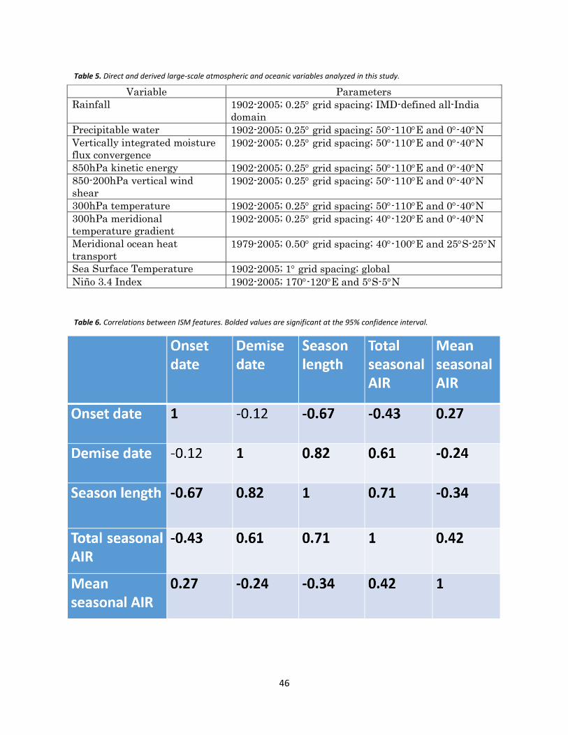
46

Variable Parameters

Rainfall 1902-2005; 0.25 grid spacing; IMD-defined all-India domain

Precipitable water 1902-2005; 0.25 grid spacing; 50-110E and 0-40N Vertically integrated moisture flux convergence

1902-2005; 0.25 grid spacing; 50-110E and 0-40N

850hPa kinetic energy 1902-2005; 0.25 grid spacing; 50-110E and 0-40N 850-200hPa vertical wind shear

1902-2005; 0.25 grid spacing; 50-110E and 0-40N

300hPa temperature 1902-2005; 0.25 grid spacing; 50-110E and 0-40N 300hPa meridional temperature gradient

1902-2005; 0.25 grid spacing; 40-120E and 0-40N

Meridional ocean heat transport

1979-2005; 0.50 grid spacing; 40-100E and 25S-25N

Sea Surface Temperature 1902-2005; 1 grid spacing; global Niño 3.4 Index 1902-2005; 170-120E and 5S-5N

Table 5. Direct and derived large-scale atmospheric and oceanic variables analyzed in this study.

Table 6. Correlations between ISM features. Bolded values are significant at the 95% confidence interval.

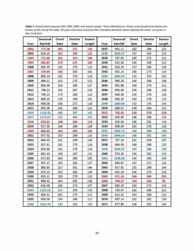
47

Table 7. A ual total seaso al AIR, AIRO, AIRD, a d seaso le gth. These I“M features’ ea s a d sta dard deviatio s are

shown at the end of the table. All years with total seasonal AIR a standard deviation above (below) the mean are given in

blue (red) font.

48

Table 7. Continued

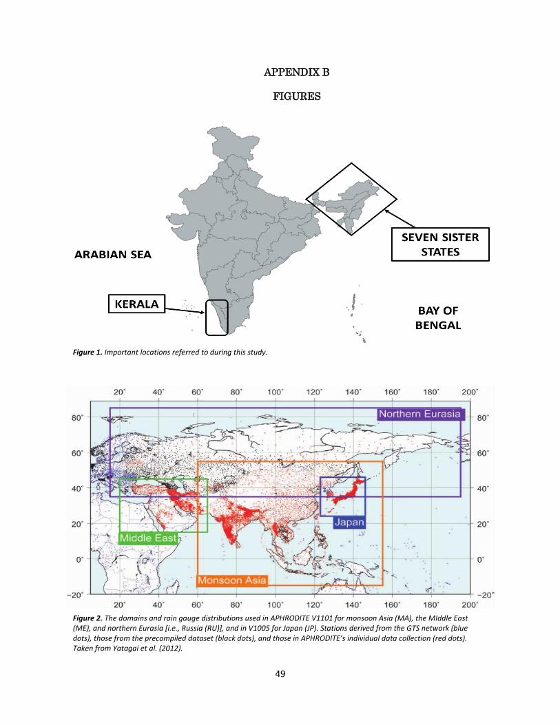
49

APPENDIX B

FIGURES

Figure 1. Important locations referred to during this study.

Figure 2. The domains and rain gauge distributions used in APHRODITE V1101 for monsoon Asia (MA), the MIddle East

(ME), and northern Eurasia [i.e., Russia (RU)], and in V1005 for Japan (JP). Stations derived from the GTS network (blue

dots), those from the precompiled dataset (black dots , a d those i APHRODITE’s i dividual data collectio red dots . Taken from Yatagai et al. (2012).

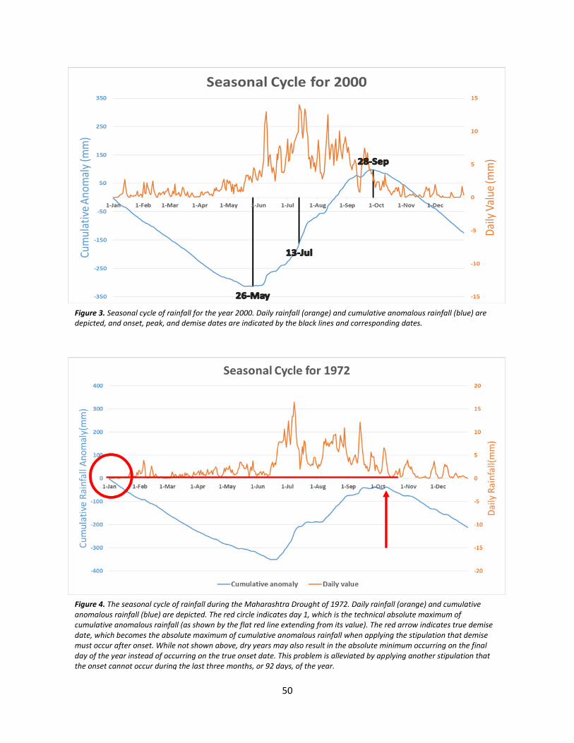
50

Figure 3. Seasonal cycle of rainfall for the year 2000. Daily rainfall (orange) and cumulative anomalous rainfall (blue) are

depicted, and onset, peak, and demise dates are indicated by the black lines and corresponding dates.

Figure 4. The seasonal cycle of rainfall during the Maharashtra Drought of 1972. Daily rainfall (orange) and cumulative

anomalous rainfall (blue) are depicted. The red circle indicates day 1, which is the technical absolute maximum of

cumulative anomalous rainfall (as shown by the flat red line extending from its value). The red arrow indicates true demise

date, which becomes the absolute maximum of cumulative anomalous rainfall when applying the stipulation that demise

must occur after onset. While not shown above, dry years may also result in the absolute minimum occurring on the final

day of the year instead of occurring on the true onset date. This problem is alleviated by applying another stipulation that

the onset cannot occur during the last three months, or 92 days, of the year.

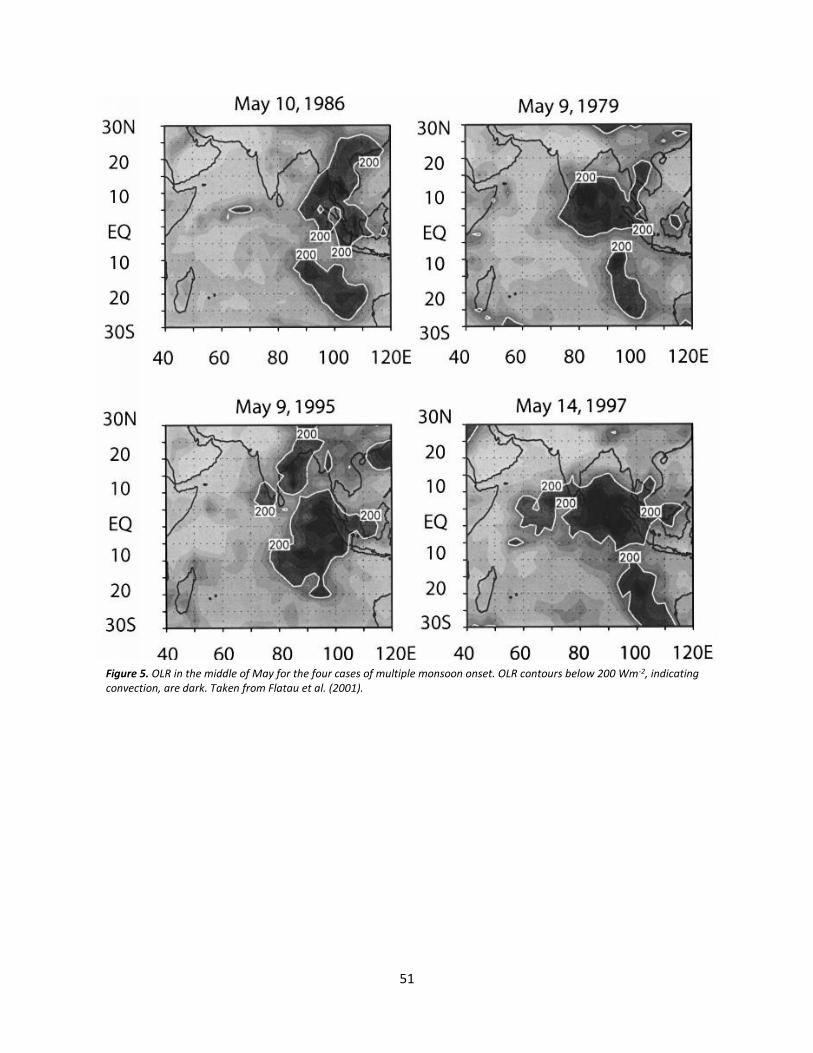
51

Figure 5. OLR in the middle of May for the four cases of multiple monsoon onset. OLR contours below 200 Wm-2, indicating

convection, are dark. Taken from Flatau et al. (2001).

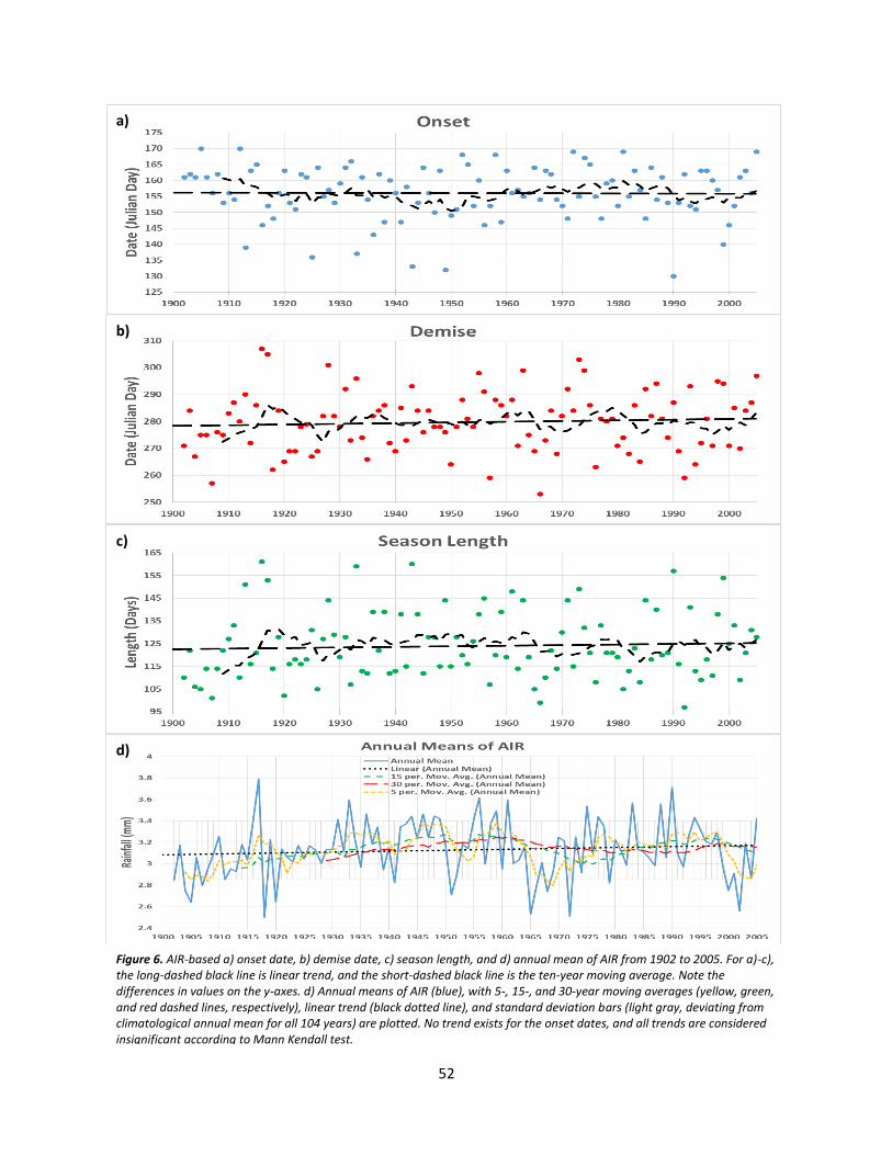
52

d)

c)

a)

b)

Figure 6. AIR-based a) onset date, b) demise date, c) season length, and d) annual mean of AIR from 1902 to 2005. For a)-c),

the long-dashed black line is linear trend, and the short-dashed black line is the ten-year moving average. Note the

differences in values on the y-axes. d) Annual means of AIR (blue), with 5-, 15-, and 30-year moving averages (yellow, green,

and red dashed lines, respectively), linear trend (black dotted line), and standard deviation bars (light gray, deviating from

climatological annual mean for all 104 years) are plotted. No trend exists for the onset dates, and all trends are considered

insignificant according to Mann Kendall test.

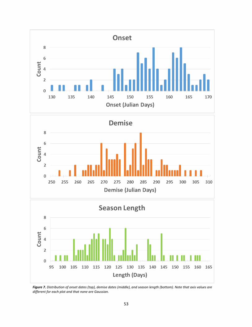
53

Figure 7. Distribution of onset dates (top), demise dates (middle), and season length (bottom). Note that axis values are

different for each plot and that none are Gaussian.

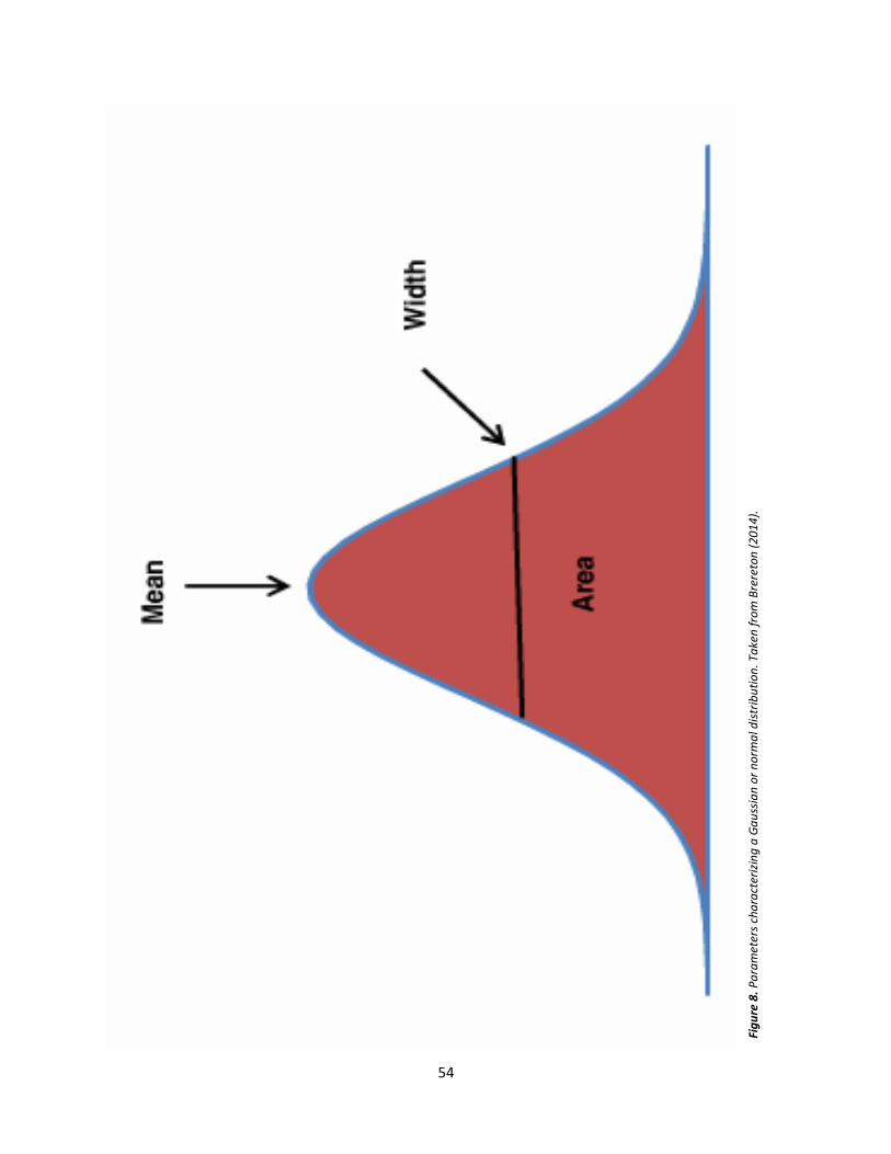
54

Fig

ure

8.

Pa

ram

ete

rs c

ha

ract

eri

zin

g a

Ga

uss

ian

or

no

rma

l d

istr

ibu

tio

n.

Ta

ke

n f

rom

Bre

reto

n (

20

14

).

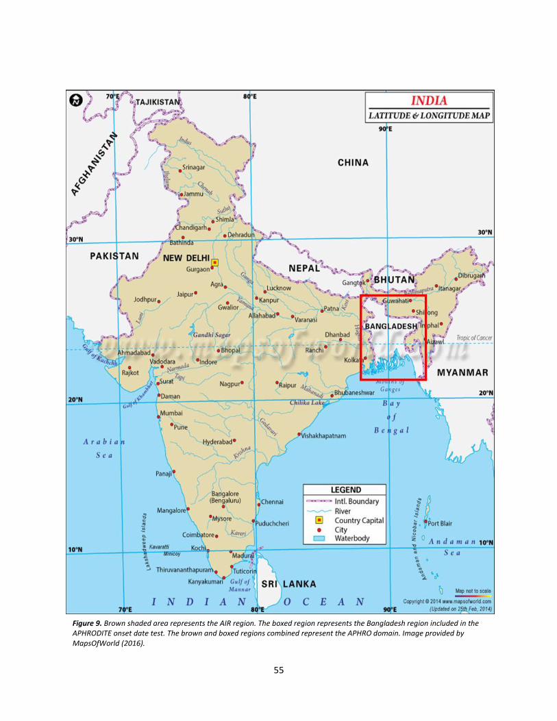
55

Figure 9. Brown shaded area represents the AIR region. The boxed region represents the Bangladesh region included in the

APHRODITE onset date test. The brown and boxed regions combined represent the APHRO domain. Image provided by

MapsOfWorld (2016).

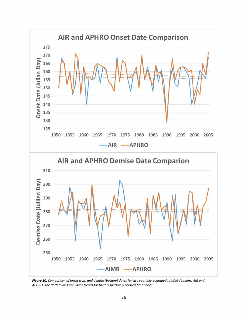
56

Figure 10. Comparison of onset (top) and demise (bottom) dates for two spatially-averaged rainfall domains: AIR and

APHRO. The dotted lines are linear trends for their respectively colored time series.

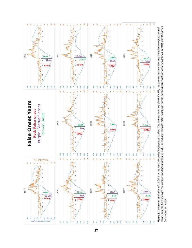
57

Fig

ure

11

. S

ea

son

al

evo

luti

on

of

11

fa

lse

on

set

ye

ars

re

cord

ed

by

pre

vio

us

stu

die

s. T

he

ora

ng

e l

ine

s a

re t

he

da

ily A

IR,

the

ora

ng

e d

ash

ed

lin

es

are

th

e c

lim

ato

log

ica

l a

nn

ua

l

me

an

, a

nd

th

e b

lue

lin

es

are

th

e c

um

ula

tive

da

ily a

no

ma

ly o

f A

IR.

Th

e r

ed

ba

rs in

dic

ate

fa

lse

on

set,

th

e p

urp

le b

ars

in

dic

ate

ac

tual

ose

t as d

efi

ne

d b

y I

MD

, a

nd

th

e g

ree

n

ba

rs r

ep

rese

nt

AIR

O.

58

Figure 12. Ekman transport throughout the mixed layer (roughly 100m) of the ocean, where the competing Coriolis force

and turbulent drag slow and turn the direction of the current to the right at deeper depths. The longest arrow is the surface

current, which flows at a 45° angle to the right of the surface winds. Although not depicted, the averaged Ekman transport

flows perpendicular to the surface winds. Taken from Ekman (1905).

Figure 13. Simplified regulation of the seasonal cycle of the Indian Ocean in the boreal a) summer and b) winter, where

black arrows indicate the direction of near-surface winds and gray arrows indicated the direction of Ekman transport and

the resulting heat flux. Adapted from Loschnigg and Webster (2000).

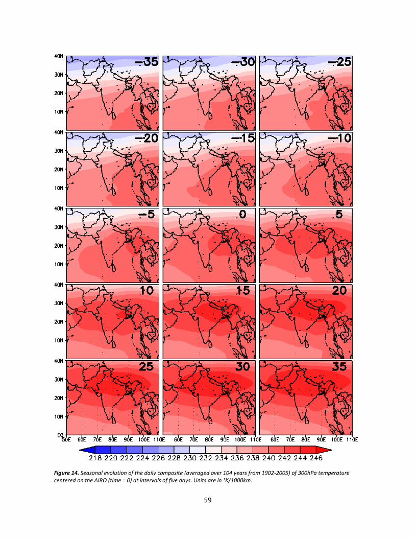
59

Figure 14. Seasonal evolution of the daily composite (averaged over 104 years from 1902-2005) of 300hPa temperature

centered on the AIRO (time = 0) at intervals of five days. Units are in °K/1000km.

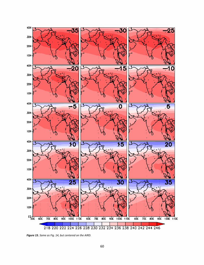
60

Figure 15. Same as Fig. 14, but centered on the AIRD.

61

b)

a)

Fig

ure

16

. T

he

cli

ma

tolo

gic

al

da

ily z

on

al p

rog

ress

ion

of

the

me

rid

ion

al

tem

pe

ratu

re g

rad

ien

t b

etw

ee

n 5

°N a

nd

25

°N a

t 3

00

hP

a a

s a

fu

nct

ion

of

lea

d/l

ag

tim

e w

ith

re

spe

ct t

o

the

a)

AIR

O a

nd

b)

AIR

D f

rom

40

°E t

o 1

20

°E.

Un

its

are

in

°K

/10

00

km

. T

he

ze

ro c

on

tou

r li

ne

is

sho

wn

in

bla

ck.

62

Figure 17. Same as Fig. 14, but for 850hPa to 200hPa vertical wind shear. Units are in ms-1.

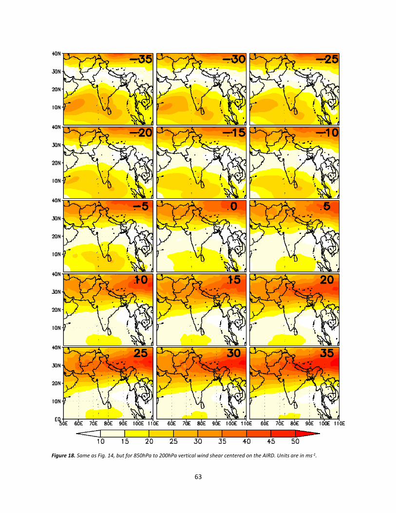
63

Figure 18. Same as Fig. 14, but for 850hPa to 200hPa vertical wind shear centered on the AIRD. Units are in ms-1.

64

Figure 19. Same as Fig. 14, but for kinetic energy of 850hPa winds. Units are in m2s-2.

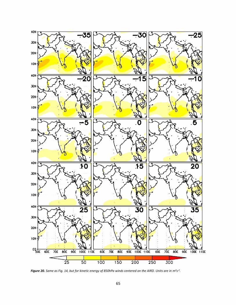
65

Figure 20. Same as Fig. 14, but for kinetic energy of 850hPa winds centered on the AIRD. Units are in m2s-2.

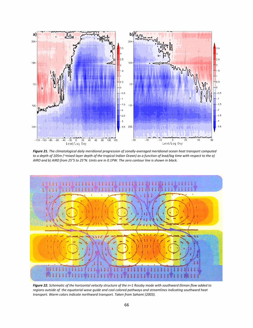
66

a) b)

Figure 21. The climatological daily meridional progression of zonally-averaged meridional ocean heat transport computed

to a depth of 105m (~mixed layer depth of the tropical Indian Ocean) as a function of lead/lag time with respect to the a)

AIRO and b) AIRD from 25°S to 25°N. Units are in 0.1PW. The zero contour line is shown in black.

Figure 22. Schematic of the horizontal velocity structure of the n=1 Rossby mode with southward Ekman flow added to

regions outside of the equatorial wave guide and cool colored pathways and streamlines indicating southward heat

transport. Warm colors indicate northward transport. Taken from Sahami (2003).

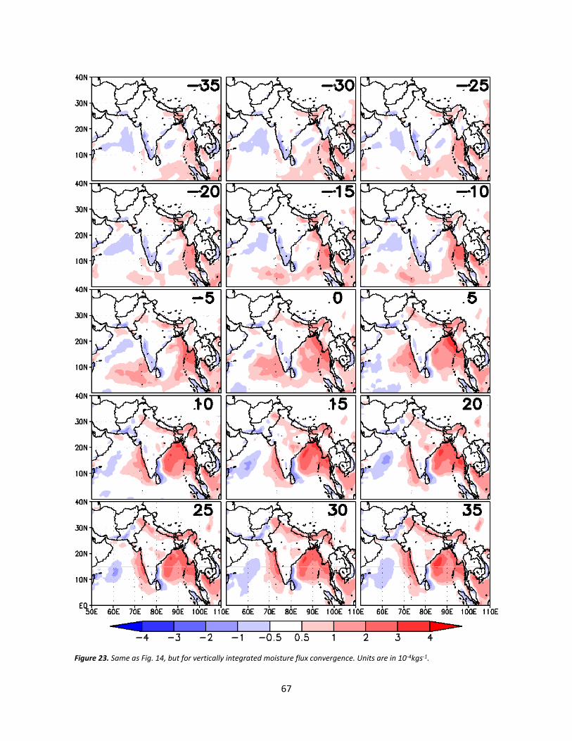
67

Figure 23. Same as Fig. 14, but for vertically integrated moisture flux convergence. Units are in 10-4kgs-1.

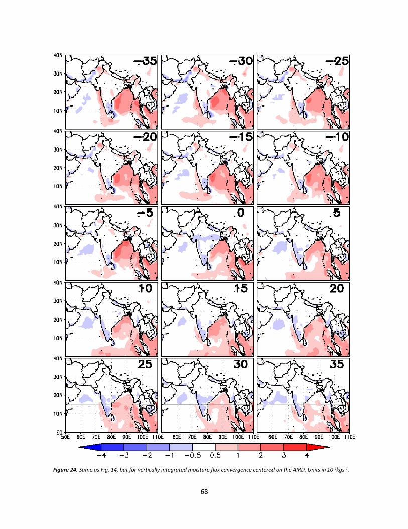
68

Figure 24. Same as Fig. 14, but for vertically integrated moisture flux convergence centered on the AIRD. Units in 10-4kgs-1.

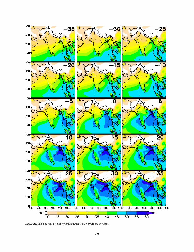
69

Figure 25. Same as Fig. 14, but for precipitable water. Units are in kgm-2.

70

Figure 26. Same as Fig. 14, but for precipitable water centered on the AIRD. Units are in kgm-2.

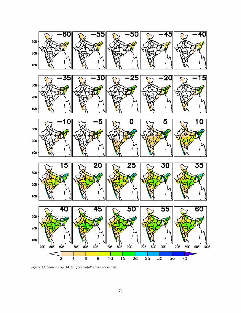
71

Figure 27. Same as Fig. 14, but for rainfall. Units are in mm.

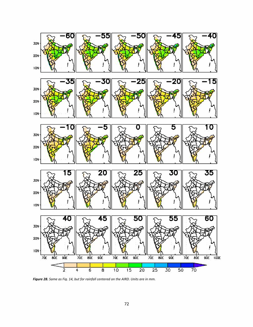
72

Figure 28. Same as Fig. 14, but for rainfall centered on the AIRD. Units are in mm.

73

a) b)

Figure 29. Correlation of a) AIRO and b) AIRD date anomalies with total seasonal rainfall anomalies. Only significant values

at 95% confidence interval are shown.

a) b)

Figure 30. Same as Fig. 29, but with 300hPa meridional temperature gradient from 5°N to 25°N at various lead/lag times

with respect to the a) AIRO and b) AIRD date.

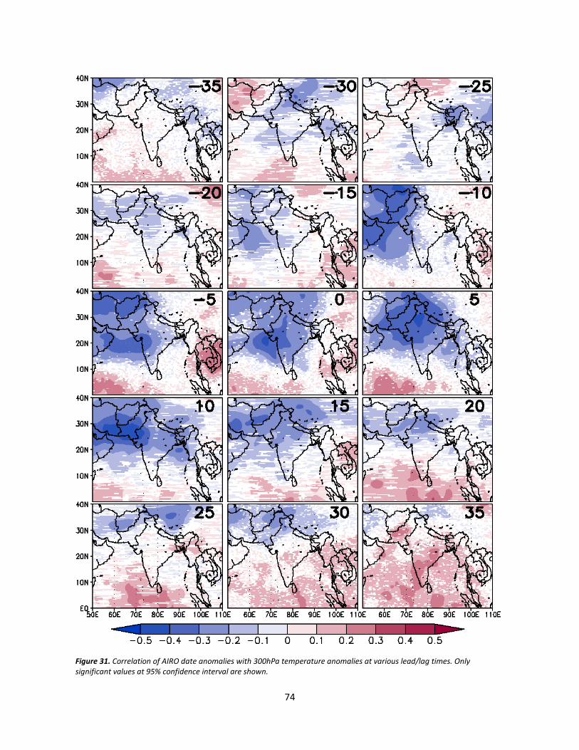
74

Figure 31. Correlation of AIRO date anomalies with 300hPa temperature anomalies at various lead/lag times. Only

significant values at 95% confidence interval are shown.

75

Figure 32. Same as Fig. 31, but with AIRD date anomalies.

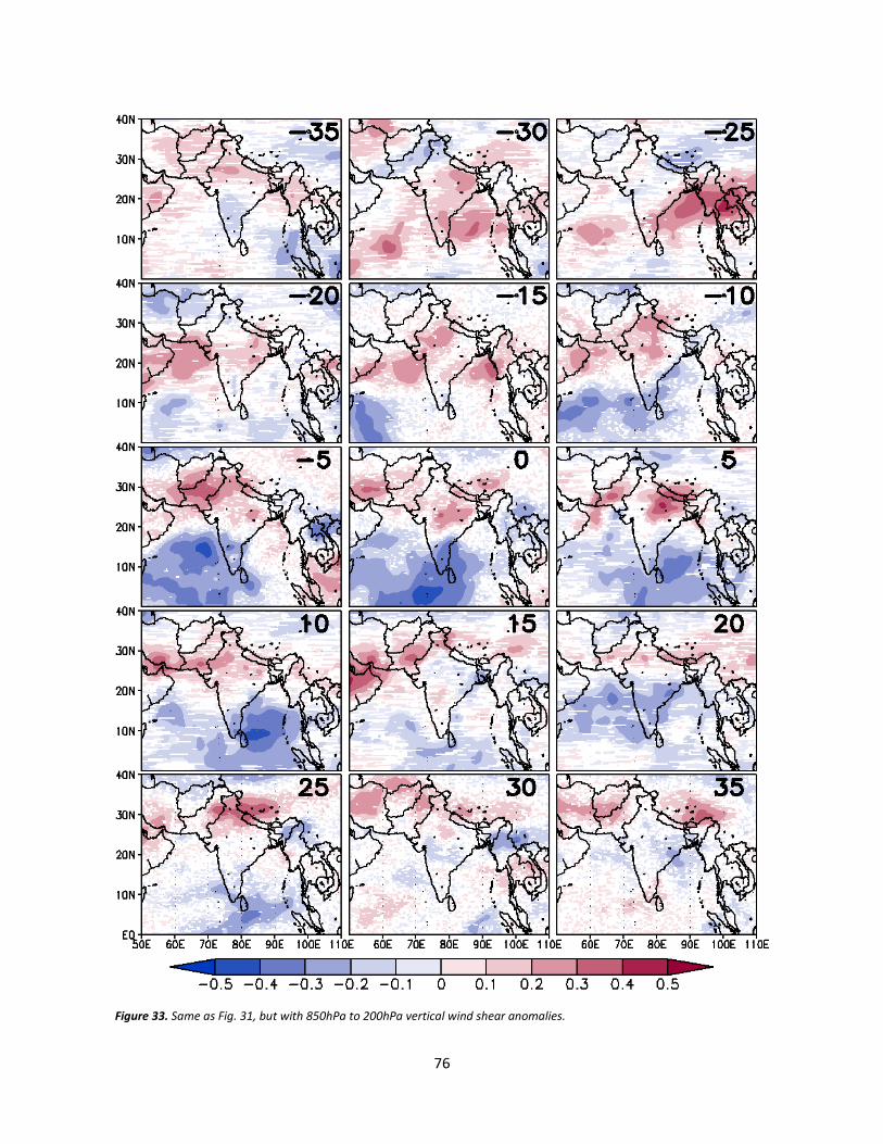
76

Figure 33. Same as Fig. 31, but with 850hPa to 200hPa vertical wind shear anomalies.

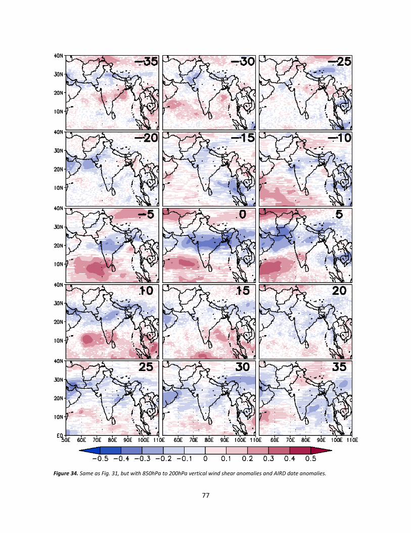
77

Figure 34. Same as Fig. 31, but with 850hPa to 200hPa vertical wind shear anomalies and AIRD date anomalies.

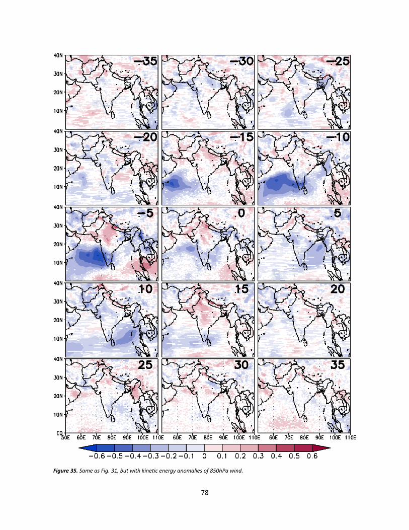
78

Figure 35. Same as Fig. 31, but with kinetic energy anomalies of 850hPa wind.

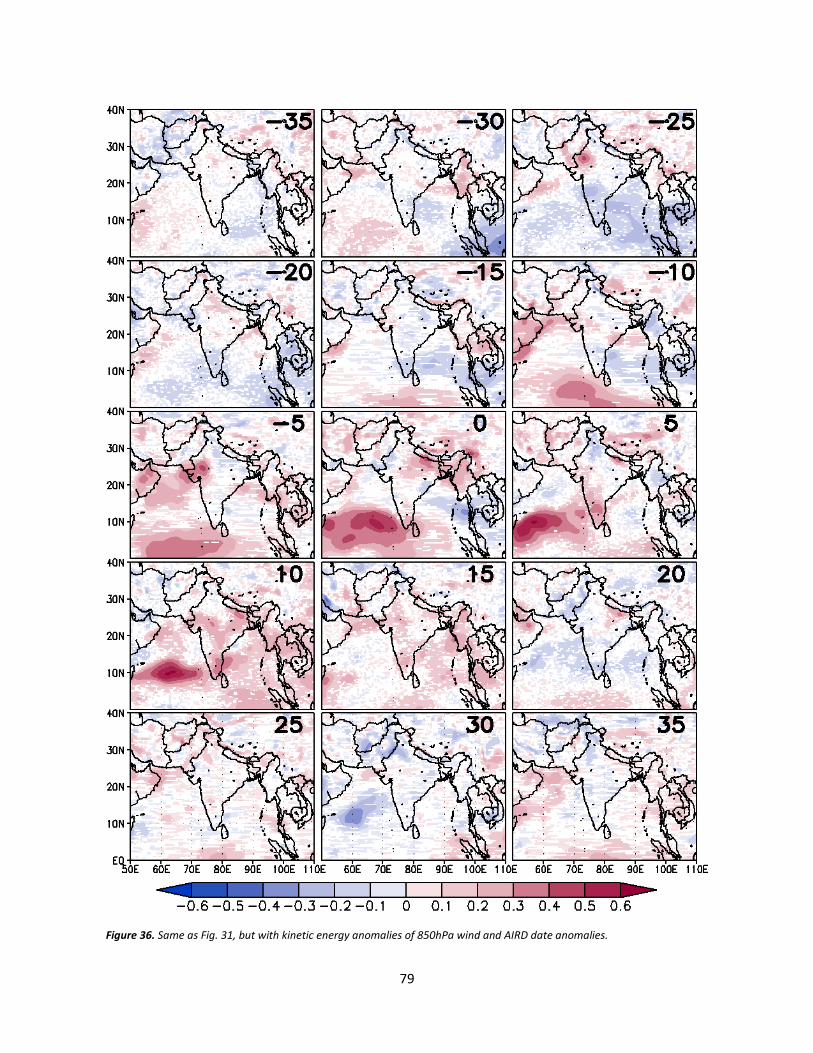
79

Figure 36. Same as Fig. 31, but with kinetic energy anomalies of 850hPa wind and AIRD date anomalies.

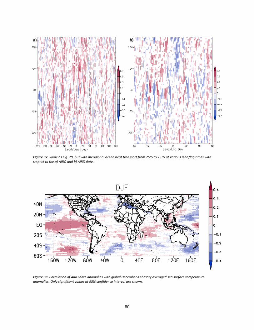
80

a) b)

Figure 37. Same as Fig. 29, but with meridional ocean heat transport from 25°S to 25°N at various lead/lag times with

respect to the a) AIRO and b) AIRD date.

Figure 38. Correlation of AIRO date anomalies with global December-February averaged sea surface temperature

anomalies. Only significant values at 95% confidence interval are shown.

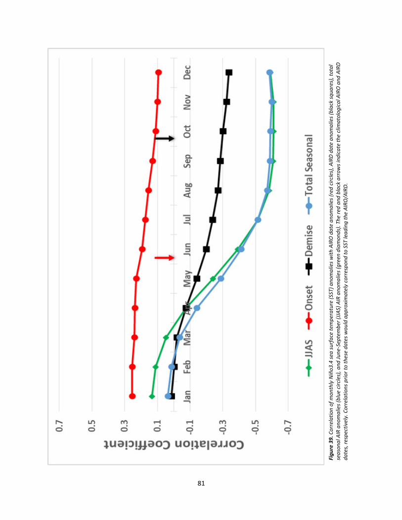
81

Fig

ure

39

. C

orr

ela

tio

n o

f m

on

thly

Niñ

o3

.4 s

ea

su

rfa

ce t

em

pe

ratu

re (

SST

) a

no

ma

lie

s w

ith

AIR

O d

ate

an

om

ali

es

(re

d c

ircl

es)

, A

IRD

da

te a

no

ma

lie

s (b

lack

sq

ua

res)

, to

tal

sea

son

al

AIR

an

om

ali

es

(blu

e c

ircl

es)

, a

nd

Ju

ne

-Se

pte

mb

er

(JJA

S)

AIR

an

om

ali

es

(gre

en

dia

mo

nd

s).

Th

e r

ed

an

d b

lack

arr

ow

s in

dic

ate

th

e c

lim

ato

log

ica

l A

IRO

an

d A

IRD

da

tes,

re

spe

ctiv

ely

. C

orr

ela

tio

ns

pri

or

to t

he

se d

ate

s w

ou

ld a

pp

roxi

ma

tely

co

rre

spo

nd

to

SS

T l

ea

din

g t

he

AIR

O/A

IRD

.

82

Fig

ure

40

. A

co

mp

ari

son

of

the

to

tal

sea

son

al

AIR

(b

lue

) a

nd

th

e J

un

e-S

ep

tem

be

r (J

JAS)

All

-In

dia

Mo

nso

on

Ra

infa

ll (

AIM

R;

ora

ng

e).

Th

e h

ori

zon

tal d

ash

ed

lin

es

wit

h

corr

esp

on

din

g c

olo

rs m

ark

on

e s

tan

da

rd d

evi

ati

on

be

low

an

d a

bo

ve t

he

ir r

esp

ect

ive

me

an

s.

83

Figure 41. Same as Fig. 31, but with vertically integrated moisture flux convergence anomalies.

84

Figure 42. Same as Fig. 31, but with vertically integrated moisture flux convergence anomalies and AIRD anomalies.

85

Figure 43. Same as Fig. 31, but with precipitable water anomalies.

86

Figure 44. Same as Fig. 31, but with precipitable water anomalies and AIRD anomalies.

87

a)

b)

Figure 45. Same as Fig. 29, but with AIR anomalies at various lead/lag times with respect to the a) AIRO and b) AIRD date.

The composite daily rainfall (blue line; units in mm) is also plotted to show the sudden increase (decrease) at the AIRO

(AIRD). Correlation coefficient is plotted as the orange line, with missing values indicating insignificance at the 95%

confidence interval.

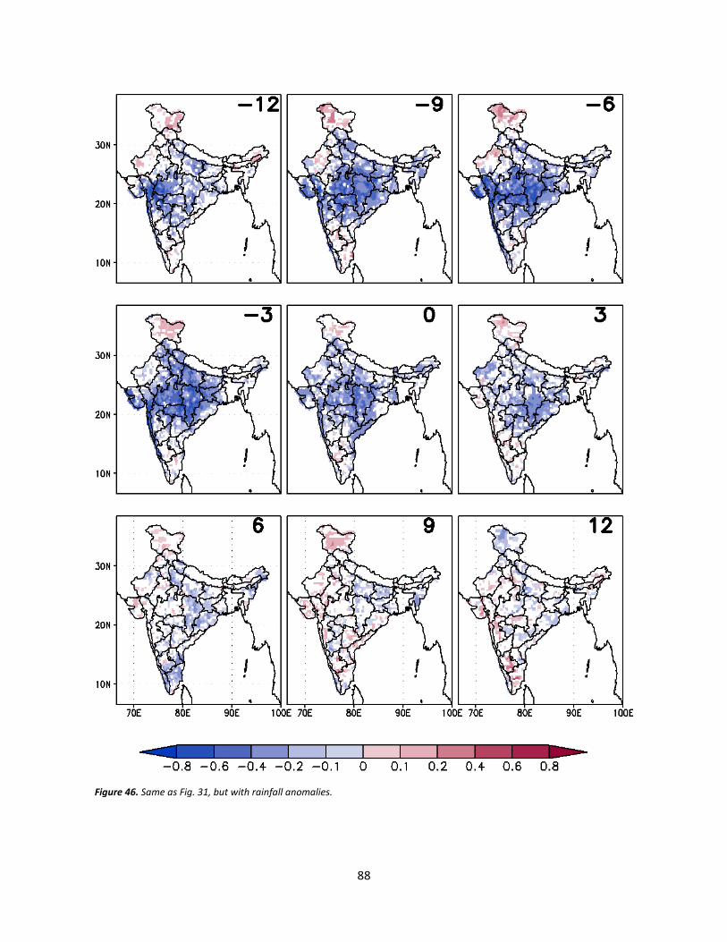
88

Figure 46. Same as Fig. 31, but with rainfall anomalies.

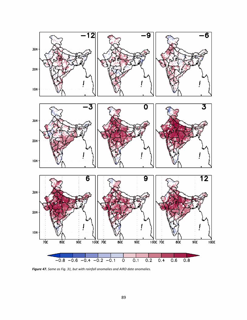
89

Figure 47. Same as Fig. 31, but with rainfall anomalies and AIRD date anomalies.

90

REFERENCES

Akuetevi, C. Q. C., B. Barnier, J. Verron, J.-M. Molines, and A. Lecointre, 2016: Interactions between the Somali Current eddies during the summer monsoon: insights from a numerical study. Ocean Sci., 12(1), 185-205, doi:10.5194/os-12-185-2016.

Ananthakrishnan, R., V. Srinivasan, A. R. Ramakrishnan, and R. Jambunathan, 1968:

Synoptic features associated with onset of southwest monsoon over Kerala. Forecast Manual, Vol.IV-18.2, India Meteorological Department.

,and M. K. Soman, 1988: The onset of the southwest monsoon over Kerala, 1901-

1980. Int. J. Climatol., 8(3), 283-296, doi:10.1002/joc.3370080305. Baquero-Bernal, A., M. Latif, and S. Legutke, 2002: On dipolelike variability of sea surface

temperature in the tropical ocean. J. Climate, 15(11), 1358-1368, doi:10.1175/1520-0442(2002)015<1358:ODVOSS>2.0.CO;2.

Beal, L. M., and K. A. Donohue, 2013: The Great Whirl: observations of its seasonal

development and interannual variability. J. Geophys. Res. Oceans. 118(1), 1-13, doi:10.1029/2012JC008198.

Bhat, G. S., 2002: Near-surface variations and surface fluxes over the northern Bay of

Bengal during the 1999 Indian summer monsoon. J. Geophys. Res. Atmos., 107(D17), doi:10.1029/2001JD000382.

Brereton, R. G., 2014: The normal distribution. J. Chemometrics, 28(11), 789-792,

doi:10.1002/cem.2655. Chernick, M. R., 2008: Bootstrap Methods: A Guide for Practitioners and Researchers,

Second Edition. Wiley, 369pp. Chirokova, G., and P. J. Webster, 2006: Interannual variability of Indian Ocean heat

transport. J. Climate, 19(6), 1013-1031, doi:10.1175/JCLI3676.1. Dee, D. P., M. Balmaseda, G. Balsamo, R. Engelen, A. J. Simmons, and J.-N. Thépaut,

2014: Toward a consistent reanalysis of the climate system. Bull. Amer. Meteor. Soc., 95(8), 1235-1248,10.1175/BAMS-D-13-00043.1.

DiCiccio, T. J., and B. Efron, 1996: Bootstrap confidence intervals. Statist. Sci., 11(3), 189-

228. Efron, B., 1979: Bootstrap methods: another look at the jackknife. Ann. Statist., 7(1), 1-26,

doi:10.1214/aos/1176344552. , 1987: Better bootstrap confidence intervals. J. Amer. Stat. Assoc., 82(397), 171-185,

doi:10.1080/01621459.1987.10478410.

91

Ekman, V. W., 1905: On the influence of the Earth’s rotation on ocean-currents. Arkiv för Matematik, Astronomi och Fysik, 2(11).

Fasullo, J., and P. J. Webster, 2003: A hydrological definition of the Indian summer

monsoon onset and withdrawal. J. Climate, 16(19), 3200-3211, doi:10.1175/1520-0442(2003)016<3200a:AHDOIM>2.0.CO;2.

Fieux, M., and H. Stommel, 1977: Onset of the southwest monsoon over the Arabian Sea

from marine reports of surface winds: structure and variability. Mon. Wea. Rev., 105(2), 231-236, doi:10.1175/1520-0493(1977)105<0231:OOTSMO>2.0.CO;2.

Flatau, M. K., P. J. Flatau, and D. Rudnick, 2001: The dynamics of double monsoon onsets.

J. Climate, 14(21), 4130-4146, doi:10.1175/1520-0442(2001)014<4130:TDODMO>2.0.CO;2.

, P. J. Flatau, J. Schmidt, and G. N. Kiladis, 2003: Delayed onset of the 2002 Indian

monsoon. Geophys. Res. Let., 30(14), doi:10.1029/2003GL017434. Fontaine, B., P.-A. Monerie, M. Gaetani, P. Roucou, 2011: Climate adjustments over the

African-Indian monsoon regions accompanying Mediterranean Sea thermal variability. J. Geophys. Res. Atmos., 116(D23), doi:10.1029/2011JD016273.

Gadgil, S., and K. R. Kumar, 2006: The Asian monsoon – agriculture and economy. The

Asian Monsoon. B. Wang, Ed., Springer Science and Business Media, 651-683. Goswami, B. N., V. Krishnamurthy, and H. Annmalai, 1999: A broad-scale circulation index

for the interannual variability of the Indian summer monsoon. Quart. J. Roy. Meteor. Soc., 125(554), 611-633, doi:10.1002/qj.49712555412.

, and K. C. Gouda, 2010: Evaluation of a dynamical basis for advance forecasting of

the date of onset of monsoon rainfall over India. Mon. Wea. Rev., 138(8), 3120-3141, doi:10.1175/2010MWR2978.1.

Guan, Y., J. Zhu, B. Huang, Z.-Z. Hu, and J. L. Kinter, 2013: South Pacific Ocean Dipole: a

predictable mode on multiseasonal time scales. J. Climate, 27(4), 1648-2658, doi:10.1175/JCLI-D-13-00293.1.

Hall, P., 1992: On bootstrap confidence intervals in nonparametric regression. Ann. Statist.,

20(2), 695-711. Hastenrath, S., and A. Rosen, 1983: Patterns of India monsoon rainfall anomalies. Tellus A,

35A(4), 324-331, doi:10.1111/j.1600-0870.1983.tb00206.x. Hsu, H.-H., C-T Terng, and C-T. Chen, 1999: Evolution of large-scale circulation and

heating during the first transition of Asian summer monsoon. J. Climate, 12(3), 793-810, doi:10.1175/1520-0442(1999)012<0793:EOLSCA>2.0.CO;2.

92

Janowiak, J. E., and P. Xie, 2003: A global-scale examination of monsoon-related precipitation. J. Climate, 16(24), 4121-4133, doi:10.1175/1520-0442(2003)016<4121:AGEOMP>2.0.CO;2.

Joseph, P. V., and P. V. Pillai, 1988: 40-day mode of equatorial trough for long-range

forecasting of Indian summer monsoon onset. Current Sci., 57, 951-954. , J. K. Eischeid, and R. J. Pyle, 1994: Interannual variability of the onset of the

Indian summer monsoon and its association with atmospheric features, El Niño, and sea surface temperature anomalies. J. Climate, 7(1), 81-105, doi:10.1175/1520-0442(1994)007<0081:IVOTOO>2.0.CO;2.

, K. P. Sooraj, and C. K. Rajan, 2006: The summer monsoon onset process over South

Asia and an objective method for the date of monsoon onset over Kerala. Int. J. Climatol., 26(13), 1871-1893, doi:10.1002/joc.1340.

Kirtman, B. P., and J. Shukla, 2000: Influence of the Indian summer monsoon on ENSO.

Quart. J. Roy. Meteor. Soc., 126(562), 213-239, doi:10.1002/qj.49712656211. Krishnamurti, T. N., and Y. Ramanathan, 1982: Sensitivity of the monsoon onset to

differential heating. J. Atm. Sci., 39(6), 1290-1306, doi:10.1175/1520-0469(1982)039<1290:SOTMOT>2.0.CO;2.

Kumar, K. K., M. K. Soman, and K. R. Kumar, 1995: Seasonal forecasting of Indian

summer monsoon rainfall: a review. Wea., 50(12), 449-467, doi:10.1002/j.1477-8696.1995.tb06071.x.

, K. R. Kumar, R. G. Ashrit, N. R. Deshpande, and J. W. Hansen, 2004: Climate

impacts on Indian agriculture. Int. J. Climatol., 24(11), 1375-1393, doi:10.1002/joc.1081.

Kumar, K. N., M. Rajeevan, D. S. Pai, A. K. Srivastava, and B. Preethi, 2013: On the

observed variability of monsoon droughts over India. Wea. and Climate Extremes, 1, 42-50, doi:10.1016/j.wace.2013.07.006.

Lau, K.-M., H.-T. Wu, and S. Yang, 1998: Hydrologic processes associated with the first

transition of the Asian summer monsoon: a pilot satellite study. Bull. Amer. Meteor. Soc., 79(9), 1871-1882, doi:10.1175/1520-0477(1998)079<1871:HPAWTF>2.0.CO;2.

Liebmann, B., S. J. Camargo, A. Seth, J. A. Marengo, L. M. V. Carvalho, D. Allured, R. Fu,

and C. S. Vera, 2007: Onset and end of the rainy season in South America in observations and the ECHAM 4.5 Atmospheric General Circulation Model. J. Climate, 20(10), 2037-2050, doi:10.1175/JCLI4122.1.

Loschnigg, J., and P. J. Webster, 2000: A coupled ocean-atmosphere system of SST

modulation for the Indian Ocean. J. Climate, 13(19), 3342-3360, doi:10.1175/1520-0442(2000)013<3342:ACOASO>2.0.CO;2.

93

Maps of World, 2016. India Latitude and Longitude Map. Accessed 14 March 2016. [Available online at http://www.mapsofworld.com/lat_long/india-lat-long.html.]

Misra, V., and S. DiNapoli, 2014: The variability of the Southeast Asian summer monsoon.

Int. J. Climatol., 34(3), 893-901, doi:10.1002/joc.3735. Montegut, C. B., G. Madec, A. S. Fischer, A. Lazar, D. Iudicone, 2004: Mixed layer depth

over the global ocean: an examination of profile data and a profile-based climatology. J. Geophys. Res. Oceans, 109(C12), doi:10.1029/2004JC002378.

Moron, V., and A. W. Robertson, 2014: Interannual variability of Indian summer monsoon

rainfall onset date at local scale. Int. J. Climatol., 34(4), 1050-1061, doi:10.1002/joc.3745.

Murakami, T., and T. Nakazawa, 1985: Transition from the Southern to Northern

Hemisphere summer monsoon. Mon. Wea. Rev., 113(9), 1470-1486, doi: 10.1175/1520-0493(1985)113<1470:TFTSTN>2.0.CO;2.

NPL, 2016. Physical properties of sea water. Accessed 14 March 2016. [Available online at

http://www.kayelaby.npl.co.uk/general_physics/2_7/2_7_9.html.] NPTEL, 2013. Seasonal transitions – Part 2: spring to summer transition. Accessed 14

March 2016. [Available online at http://nptel.ac.in/courses/119108006/17.] Pai, D. S., and M. Rajeevan, 2009: Summer monsoon onset over Kerala: new definition and

prediction. J. Earth Syst. Sci., 118(2), 123-135, doi:10.1007/s12040-009-0020-y. , L. Sridhar, M. Rajeevan, O. P. Sreejith, N. S. Satbhai, and B. Mukhopadhyay,

2014a: Development of a new high spatial resolution (0.25°x0.25°) long period (1901-2010) daily gridded rainfall data set over India and its comparison with existing data sets over the region. Mausam, 65(1), 1-18.

, L. Sridhar, M. R. Badwaik, and M. Rajeevan, 2014b: Analysis of the daily rainfall

events over India using a new long period (1901-2010) high resolution (0.25°x0.25°) gridded rainfall data set. Climate Dyn., 45(3-4), doi:10.1007/s00382-014-2307-1.

Parthasarathy, B., and G. B. Pant, 1985: Seasonal relationships between Indian summer

monsoon rainfall and the Southern Oscillation. J. Climatol., 5(4), 369-378, doi:10.1002/joc.3370050404.

, N. A. Sontakke, A. A. Munot, and D. R. Kothawale, 1990: Vagaries of Indian

monsoon rainfall and its relationship with regional/global circulations. Mausam, 41(2), 301-308.

Poli, P., and Coauthors, 2013: The data assimilation system and initial performance

evaluation of the ECMWF pilot reanalysis of the 20th-century assimilating surface observations only (ERA-20C). ERA Report Series, 14.

94

, H. Hersbach, P. Berrisford, D. Dee, A. Simmons, and P. Laloyaux, 2015: ERA-20C deterministic. ERA Report Series, 20.

Prasad, V. S., and T. Hayashi, 2005: Onset and withdrawal of Indian summer monsoon.

Geophys. Res. Let., 32(20), doi:10.1029/2005GL023269. Rajeevan, M., J. Bhate, and A. K. Jaswal, 2008: Analysis of variability and trends of

extreme rainfall events over India using 104 years of gridded daily rainfall data. Geophys. Res. Let., 35(18), doi:10.1029/2008GL035143.

Ramage, C. S., 1971: Monsoon Meteorology Vol. 15. Academic Press, 296 pp. Rao, Y. P., 1976: Southwest Monsoon. India Meteorological Department, 367 pp. Rayner, N. A., D. E. Parker, E. B. Horton, C. K. Folland, L. V. Alexander, D. P. Rowell, E.

C. Kent, and A. Kaplan, 2003: Global analyses of sea surface temperature, sea ice, and night marine air temperature since the late nineteenth century. J. Geophys. Res. Atmos., 108(D14), doi:10.1029/2002JD002670.

Reynolds, R. W., T. M. Smith, C. Liu, D. B. Chelton, K. S. Casey, and G. Schlax, 2007: Daily

high-resolution-blended analyses for sea surface temperature. J. Climate, 20(22), 5473-5496, doi:10.1175/2007JCLI1824.1.

Saha, S., and Coauthors, 2010: The NCEP Climate Forecast System Reanalysis. Bull.

Amer. Meteor. Soc., 91(8), 1015-1057, doi:10.1175/2010BAMS3001.1. Sahami, K., 2003: Aspects of the heat balance of the Indian Ocean on intra-annual and

interannual time scales. Ph.D. dissertation, The University of Colorado, 191 pp. Sneyers, R., 1990: On the Statistical Analysis of Series of Observations. World

Meteorological Organization, 192 pp. Soman, M. K., and K. K. Kumar, 1993: Space-time evolution of meteorological features

associated with the onset of Indian summer monsoon. Mon. Wea. Rev., 121(4), 1177-1194, doi:10.1175/1520-0493(1993)121<1177:STEOMF>2.0.CO;2.

Sun, S., Y. Fang, L. Feng, and Tana, 2014: Influence of the Indian Ocean Dipole on the

Indian Ocean meridional heat transport. J. Marine Sys., 134, 81-88, doi:10.1016/j.jmarsys.2014.02.013.

Taniguchi, K., and T. Koike, 2006: Comparison of definitions of Indian summer monsoon

onset: better representation of rapid transitions of atmospheric conditions. Geophys. Res. Let., 33(2), doi:10.1029/2005GL024526.

Trenberth, K. E., and D. P. Stepaniak, 2001: Indices of El Niño Evolution. J. Climate, 14(8),

1697-1701, doi:10.1175/1520-0442(2001)014<1697:LIOENO>2.0.CO;2. Wang, B., Q. Ding, and P. V. Joseph, 2009: Objective definition of the Indian summer

monsoon onset. J. Climate, 22(12), 3303-3316, doi: 10.1175/2008JCLI2675.1.

95

Webster, P. J., and S. Yang, 1992: Monsoon and ENSO: selectively interactive systems.

Quart. J. Roy. Meteor. Soc., 118(507), 877-926, doi:10.1002/qj.49711850705. Wilkes, D., 2011: Statistical Methods in the Atmospheric Sciences, 2nd Edition. Academic

Press, 704pp. Wu, G., and Y. Zhang, 1998: Tibetan Plateau forcing and the timing of the monsoon onset

over South Asia and the South China Sea. Mon. Wea. Rev., 126(12), 913-927, doi:10.1002/joc.1082.

Wu, Z., and N. E. Huang, 2009: Ensemble Empirical Mode Decomposition: a noise-assisted

data analysis method. Adv. Adapt. Data Anal., 1(1), 1-41, doi:10.1142/S1793536909000047.

Xavier, P. K., C. Marzin, and B. N. Goswami, 2007: An objective definition of the Indian

summer monsoon season and a new perspective on the ENSO-monsoon relationship. Quart. J. Roy. Meteor. Soc., 133(624), 749-764, doi:10.1002/qj.45.

Yanai, M., C. Li, and Z. Song, 1992: Seasonal heating of the Tibetan Plateau and its effects

on the evolution of the Asian summer monsoon. J. Meteor. Soc. Japan, 70(1), 319-351.

Yatagai, A., K. Kamiguchi, O. Arakawa, A. Hamada, N. Yasutomi, and A. Kitoh, 2012:

APHRODITE: Constructing a long-term daily gridded precipitation dataset for Asia based on a dense network of rain gauges. Bull. Amer. Meteor. Soc., 93(9), 1401-1415, doi:10.1175/BAMS-D-11-00122.1.

Zeng, X., and E. Lu, 2004: Globally unified monsoon onset and retreat indexes. J. Climate,

17(11), 2241-2248, doi:10.1175/1520-0442(2004)017<2241:GUMOAR>2.0.CO;2.

96

BIOGRAPHICAL SKETCH

Education Florida State University, Tallahassee, Fl. – May 2016

M.S. Meteorology; Cum Laude; GPA: 3.88

Dean’s list (2014-2016) Thesis: Characterizing the onset and demise of the Indian summer monsoon

Virginia Tech, Blacksburg, Va. – May 2014 B.S. Meteorology, Magna Cum Laude; GPA: 3.65 Dean’s list (2010, 2012-2014)

Research Topics

Characteristics of onset and demise of the Indian summer monsoon

Precipitation characteristics in the visible, infrared, and microwave spectra Brownian motion

Aerosol-monsoon relationship

FSTRC radiation model analysis Atlantic warm pool influence on hurricane track

Latent heat contribution to Florida precipitation (Evaporation-precipitation feedback)

ENSO-East Pacific warm pool relationship

Atmospheric impacts on oceanic salinity variability

Scale analysis of observational parameterization on modeled flux variability Dual-Polarization winter precipitation detection

Professional Experience Florida State University, Tallahassee, Fl. ............................................................ 2015 to 2016

Meteorology Graduate Research Assistant [20hr/wk] Conducted research characterizing the onset and demise of the Indian summer monsoon to improve the lead time and accuracy of monsoon forecasting. Included professional collaboration, programming and plot production, critical thinking and analysis of unique data, and communication of novel results.

Florida State University, Tallahassee, Fl. ............................................................ 2014 to 2015 Meteorology Graduate Teaching Assistant [20hr/wk]

Assisted professor with educating and evaluating students by tutoring students on an individual need basis, leading classroom review in the professor’s absence, and grading/commenting homework.

Bus Transit, Blacksburg, Va. ................................................................................ 2012 to 2014 Bus Operator [13hr/wk] Transported passengers in a safe and timely manner, worked with 35 to 70 foot vehicles that require a Commercial Driver’s License (CDL).

Virginia Tech Writing Center, Blacksburg, Va. ................................................................. 2013 Writing Coach [5hr/wk] Guided students, including many ESL speakers, in improvement of their written communication and facilitated their linguistic competency; also corrected grammatical and syntactical errors.

97

Leadership/Volunteer Experience Go2 Church, Tallahassee, Fl. ................................................................................ 2015 to 2016 Production/Vocalist team member

Oversaw light, sound, and media production in such a manner as to reduce distraction and facilitate an atmosphere of worship. Also led congregation in worship through song.

Earth, Ocean, and Atmospheric Sciences Thalassic Society, Tallahassee, Fl. .... 2015 to 2016 Treasurer [5hr/mo] Managed the organization’s funds to ensure fiscal responsibility, thus enabling current events and setting aside additional funds for future years.

Special Olympics Florida, Tallahassee, Fl. ........................................................................ 2015 Soccer unified partner/volunteer [3 weeks, 2.5hr/wk; for State Olympics, 15hr/day]

Assisted athletes in soccer practices and games as a player and mentor; also participated as a player, chaperone, and friend of athletes in the 2015 State Summer Special Olympics, where our team won a bronze medal.

Life Center Academy, Jaipur, Rajasthan, India ................................................................ 2013 Kindergarten teaching assistant [3 weeks, 30hr/wk] Primary objectives included teaching English numbers, letters, songs, and poems to impoverished Banjara children; enabling them to produce poems and songs of their own creative expression; and offering attention, care, and friendship rarely experienced outside of their school experience.

College of Natural Resources and Environment Leadership Institute, Blacksburg, Va. ...................................................................................................... 2012 to 2013

Cohort member [8hr/wk] Applied leadership principles to team projects; learned how leaders deal with change, teamwork, and conflict; leveraged personality types to work with and lead others; and networked with environmental leaders at state and national levels in both the private and public sectors.

Chi Alpha Christian Fellowship, Blacksburg, Va. ................................................ 2012 to 2013 International student leader [3hr/wk]

Facilitated relationship and communication between international students, encouraging conversation about significant life issues and cultural diversity.

Chi Alpha Christian Fellowship, Blacksburg, Va. ................................................ 2011 to 2012 Small group/ bible study leader [5hr/wk]

Other Experience National Weather Service, Blacksburg, Va. ...................................................................... 2014

Intern [10hr/wk] National Weather Service, Blacksburg, Va. ......................................................... 2013 to 2014

Researcher (Dual-Polarization Winter Precipitation Detection) [8hr/wk] Virginia Tech, Blacksburg, Va. .......................................................................................... 2013

Midwest storm chase member [12 days] Virginia Tech Writing Center, Blacksburg, Va. ................................................................. 2012

Writing center intern [5hr/wk] Virginia Tech, Blacksburg, Va. .......................................................................................... 2011

Intramural soccer team member [1hr/wk] Professional Organizations

98

American Meteorological Society .......................................................................... 2015 to 2016 Chi Epsilon Pi Meteorology Honor Society ........................................................... 2015 to 2016 Earth, Ocean, and Atmospheric Sciences Thalassic Society ................................ 2015 to 2016 Computer Skills Programming languages

FORTRAN, GrADS (proficient) Matlab, shell scripting (elementary)

Operating systems Windows (excellent) Mac, Linux (proficient)

Other software Excel, PowerPoint, Word, Google Earth (excellent) ArcGIS, ESRI (elementary)

Language Experience Virginia Tech, Blacksburg, Va.

Ancient Greek [two semesters] Virginia Hummel Book Prize for Excellence in Ancient Greek (2014)

Life Center Academy, Jaipur, Rajasthan, India Hindi [three weeks]

Travelled to India Warhill High School, Williamsburg, Va.

Spanish [four years] Travelled to Costa Rica and Honduras [two and a half weeks]